1. Introduction
Currently, seismic inversion has become a standard procedure whose primary result is a detailed model of the elastic parameters of the geological environment. Particularly, this model enables the prediction of reservoir properties [
1,
2]. Advanced seismic inversion algorithms, including sparse-layer inversion, can generate highly detailed high-frequency models [
3,
4]. Recent research has developed inversion methods capable of robustly reconstructing multiple elastic parameters [
5].
Seismic inversion is formally defined as an algorithm that transforms a time-domain or migrated-time seismic section into an acoustic impedance section [
1,
6]. The input data for inversion typically consist of time-processed seismic results, including both pre-stack and post-stack data [
7,
8]. In areas with complex geology, depth seismic data processing is necessary to construct an accurate reservoir structural image before applying seismic inversion. In such cases, depth-migrated images are first transformed to the time domain where conventional inversion algorithms are implemented. However, standard seismic inversion relies on a one-dimensional convolutional model that assumes horizontal medium layering [
1,
6]. This assumption may not hold in practice due to various lateral heterogeneities.
The study [
9] numerically examines the applicability of seismic inversion for laterally heterogeneous media. Using two-dimensional synthetic models, it demonstrates that one-dimensional convolution modeling results match two-dimensional convolution modeling with acceptable accuracy (within 2–3 percent, including depth-to-time transformation errors). This agreement holds for both horizontally layered models and those with dipping reflectors. Consequently, one-dimensional inversion can be reliably applied to true-amplitude depth migration results for model reconstruction from reflected waves.
A crucial requirement for any inversion algorithm is its reliability in solving inverse problems. When treating seismic inversion as a tool for medium reconstruction from seismic images, it must produce physically plausible solutions despite noise, outliers, and measurement errors. Additionally, incorporating a priori geological knowledge is essential—particularly recognizing that geological environments often exhibit discontinuous property distributions. Also, inversion methods can enhance robustness through data-driven optimization approaches, such as those used in corrosion diagnostics [
10].
The choice of
norm [
4,
11,
12,
13] facilitates such reconstructions while providing greater robustness against data outliers compared to the
norm. Using
norm constraints in the optimization problem formulation allows us to enforce prior knowledge about the model. However, this approach introduces nonlinearity into the problem, necessitating advanced optimization methods. Alternative commercially successful approaches include model-based inversion methods [
14], which gradually update models while incorporating low-frequency trends, thereby ensuring synthetic-to-observed trace matching. While these linear methods simplify optimization, their reliance on the
norm makes them sensitive to outliers and may yield unfocused solutions. In this work we implement a new improved version of constrained total variation acoustic seismic inversion algorithm presented in [
11] that reconstructs sparse reflection coefficient models while preserving low-frequency trends and spatial solution continuity.
Key differences from the algorithm presented in [
11] include (a) the use of a spatial connectivity regularization term; (b) the application of a quasi-Newton optimization method instead of iteratively re-weighted least squares (IRLS); and (c) the replacement of the non-differentiable objective function (due to the
norm) with a differentiable approximation. The primary reason for adding another regularization term to the objective function is to overcome the limitations of the one-dimensional convolution model underlying seismic inversion algorithms. A one-dimensional formulation implies that neighboring reflection coefficient traces contain no information about each other. However, the spatial connectivity constraint enforces the reconstructed impedance model to exhibit slowly varying properties in the lateral direction. Computational efficiency is maintained through a quasi-Newton optimization method, which avoids solving linear systems at each iteration and requires only gradient calculations [
15,
16]. This approach converges faster than gradient descent by incorporating curvature information via Hessian estimation from previous gradients. The
norm introduces non-differentiability in the objective function due to terms involving
. In our implementation, we replace these terms with the approximation
, ensuring the objective function remains smooth and suitable for quasi-Newton optimization.
Prior to seismic inversion, true-amplitude migration of seismic data must be performed. Currently, numerous algorithms exist for true-amplitude migration, with the most widely used being Kirchhoff migration [
17], Gaussian beam migration [
18], and reverse time migration (RTM) [
19]. The applicability of these methods depends on their underlying principles: Kirchhoff migration, based on ray theory, has the most limited applicability. Gaussian beam migration offers broader applicability due to its use of beam-based wavefield extrapolation. RTM provides the most accurate results, as it employs finite-difference modeling for full-wavefield simulation. However, RTM faces challenges in preserving true amplitudes, prompting researchers to develop improved versions using linearized inversion [
20] and ray-Kirchhoff approximations [
21]. In this study, we employ Gaussian beam migration [
18], which strikes an optimal balance between computational efficiency and image quality—it is significantly faster than RTM while producing superior results compared to Kirchhoff migration.
By combining seismic inversion and depth migration, we propose a new iterative migration–inversion algorithm. While applying inversion after migration is not novel, the innovative aspect is the iterative migration–inversion approach that enables reconstruction of depth velocity models. Existing methods that also employ migration for velocity model reconstruction include migration-based travel time (MBTT) [
22] and migration velocity analysis (MVA) [
23]. These methods can recover the low-frequency component of the model but rely solely on kinematic wave-field features. In contrast, our proposed algorithm exploits dynamic wave-field properties. Similarly, reflection full-waveform inversion (RFWI) exploits dynamic wave-field properties and can effectively reconstruct velocity models, including low-frequency components [
24]. Modern full-waveform inversion (FWI) implementations aim to reconstruct broad spatial spectra of subsurface models by integrating macro-scale velocity model building with high-resolution migration imaging [
25]. Recent advances have extended FWI to multi-parameter inversion [
26] and complex geological settings with high-contrast salt bodies. However, RFWI requires computationally expensive least-squares reverse time migration (LSRTM) at each iteration to generate true-amplitude images. Our algorithm combines 1D seismic inversion and beam migration, which offers significantly faster operation.
Thus, we develop and investigate new iterative joint seismic inversion and migration algorithm for the depth velocity model reconstruction. Numerical studies examine the algorithm’s performance for both known and unknown density cases, proposing empirical relationships (e.g., Gardner’s equation) for initial impedance estimation. Validation employs synthetic data from finite-difference modeling and the realistic Marmousi model.
2. Constrained Total Variation Inversion
Acoustic seismic inversion is based on a one-dimensional convolution model [
1,
6]. This formulation assumes that for a layered model of a medium with normal incidence of a plane pressure wave the reflected wave field in the time domain can be represented as a convolution of the reflection coefficient trace with a seismic impulse. The corresponding equation has the form
where
is the seismic trace,
is the seismic impulse,
is the reflection coefficient trace. The reflection coefficient at the boundary between layers
and
i is defined as
where
is the acoustic impedance of layer
i. To discretize the Equation (
1) consider a uniform grid of
n nodes on the time axis with a step size of
from 0 to
. Let the seismic impulse be given on a uniform grid of
nodes with the same step size
from
to
and determined by the values
. Then Equation (
1) is represented as a system of linear algebraic equations and can be written as
where
is a real-valued
n-by-
n matrix of the form
The solution of the seismic inversion problem is non-unique, so it is necessary to incorporate a priori information to successfully reconstruct a physically meaningful solution. We achieve that through regularization. We reformulate problem (
1) as the minimization of an objective function comprising two components: the residual between synthetic and observed seismic traces and regularization terms that incorporate a priori information about the solution. Next, we explore the use of regularization to incorporate various forms of prior knowledge about the solution and construct the corresponding objective function.
First, assuming that the medium consists of a finite number of layers with homogeneous properties, the definition of the reflection coefficient (
2) suggests that sparse reflection coefficient traces containing a relatively small number of non-zero components are preferable. This property can be enforced using zero-order and first-order total variation regularization terms defined as
The gradient of reflection coefficient trace
is approximated numerically as
, where
is the following differentiation matrix:
The choice of
norm facilitates the reconstruction of the solution with the least number of non-zero elements.
Secondly, seismic traces lack information of the low-frequency model component. Within the framework of the low-contrast approximation of the reflection coefficients [
7,
8], which takes the form
we can construct the regularization term incorporating the low-frequency initial impedance model. Equation (
7), valid for
[
27], establishes a linear relationship between the reflection coefficient and the logarithm of the impedances. Assuming the acoustic impedance in the upper layer
is known, we express the impedance logarithms in (
7) in terms of reflection coefficients yielding the formula
where
is the integration matrix and
is the vector of logarithms of relative initial acoustic impedance given by
Note that
is proportional to the logarithm of the acoustic impedance,
. The regularization term incorporating the low-frequency initial impedance model is constructed as
Thirdly, since we are dealing with the one-dimensional convolution model, it is necessary to consider neighboring traces to ensure the spatial connectivity in the solution. When addressing a 2D profile or 3D model, the acoustic impedance reconstruction is performed trace by trace. In practical cases where seismic images contain noise, an approach that ignores neighboring traces produces undesired artifacts, such as <<vertical lines>> (an example is presented in the
Section 5). To overcome this issue we add a constraint to the objective function that penalizes the solution deviating significantly from the neighboring trace. Suppose the inversion is already complete for a neighboring trace and its reflection coefficient trace
is known. The solution for the current trace will resemble
in reflection coefficient values, but layer border positions may differ if the borders are non-horizontal. Hence, the difference
may not be small. Referring again to the low-contrast approximation (
7), the product
is proportional to the logarithm of the acoustic impedance
, so
exhibits a block structure, while
r has a spike structure. Consequently, the difference
remains small for similar reflection coefficient traces even if they have different border positions. We propose to take into account the neighboring traces via the regularization term of the form
where
is the previously found solution for the neighboring trace. Preserving the potential for parallelization in seismic inversion is crucial. Typically, inversion is performed on a regular rectangular grid where each point contains a seismic trace for inversion. We propose a two-step inversion approach. First, we invert selected traces on a coarse grid without considering neighboring traces. This step can be executed in parallel since these traces are sufficiently distant from each other, making neighbor information unnecessary. Next, we invert all remaining traces using the nearest trace from the first step as a neighbor. An alternative implementation involves using multiple neighboring traces
with a weighted sum of terms as in Equation (
11). This spatial continuity regularization enables reconstruction of the acoustic impedance model while eliminating artifacts caused by the one-dimensional inversion formulation and maintaining the capability for parallel computation.
Finally, the objective function of the constrained total variation inversion has the form
where
are regularization parameters. It is important to note that the low-contrast approximation (
7) is only used to incorporate a priori information about the initial impedance model and neighboring traces and it is not used in the direct modeling of the synthetic seismic trace according to Formula (
1). Following [
11], we use the
norm instead of the
norm in the residual term as it allows us to negate the influence of the outliers present in seismic data. The minimization of the objective function is performed using the quasi-Newton method BFGS, which requires the computation of the gradient of the objective function (
12). The acoustic impedance trace is then reconstructed using the recurrent relation (
2) after determining the reflection coefficients and the acoustic impedance in the upper layer. Non-differentiable terms in the form of
are approximated as
with small value
to ensure smoothness of the objective function. The minimization procedure requires initial determination of regularization parameters
. We propose using a generalized
L-curve framework algorithm [
28] that computes near-optimal values for multiple regularization parameters through fixed-point iteration. For seismic inversion applications, we recommend determining these parameters on a coarse grid using only 5–10% of seismic traces. Once established on the coarse grid, the parameters can be spatially interpolated to obtain a complete parameter distribution across the study area. This approach significantly reduces computational costs associated with the fixed-point iteration procedure [
28] while maintaining near-optimal regularization parameters for each seismic trace in the inversion process.
Traditionally, seismic inversion is applied in the time domain. To apply it to the results of depth-domain seismic data processing, a <<depth-to-time>> transform is proposed. This transform establishes a connection between the depth scale and the time scale using the following equation:
where
t is time,
z is depth, and
is the initial velocity model in the depth scale. Before applying seismic inversion to the results of depth-domain seismic data processing, the seismic traces and the initial acoustic impedance model are converted to the time scale using the initial velocity model according to Formula (
13). The inversion is performed in the time domain and the results are then converted back to the depth scale.
The proposed seismic inversion algorithm is capable of reconstructing a sparse reflection coefficient model while accounting for the initial acoustic impedance model and neighboring traces. The reconstructed model may exhibit more focused impedance anomalies since the seismic inversion algorithm tends to recover as few reflecting borders as possible. However, this approach typically provides slightly inferior vertical resolution and thin-layer detection capability compared to model-based inversion methods [
29,
30]. Consequently, the selected seismic inversion method proves particularly effective for cases involving substantial impedance contrasts between adjacent layers.
3. True Amplitude Depth Migration
As a true amplitude migration method, Gaussian beam imaging technology is used as a basis. This approach enables the construction of images of reflecting or scattering objects with a high signal-to-noise ratio [
18]. Wave seismic images are constructed in true amplitudes meaning that their amplitudes are proportional to the linearized reflection coefficient. To achieve this, the wave field is represented as a superposition of Gaussian beams. This ensures uniform resolution across the entire section, which is accomplished by automatically selecting weights within the algorithm so that the same Gaussian beams are chosen at the image points, while on the observation surface these Gaussian beams vary depending on the depth and angle of inclination. To speed up calculations, a simpler approach can be employed where Gaussian beams are chosen to be the same on the surface and compensation for geometric weight differences is added. This results in an analog of Kirchhoff migration in structural angles [
17] with additional data summation. Since the procedure is implemented in structural angles, it is possible to obtain an image for the zero opening angle which corresponds to the normal incidence of a wave with a reflection coefficient matching the acoustic case of seismic inversion. Thus, the following visualization condition is used to construct a depth image in true amplitudes [
18]:
where
d is seismic data,
is source coordinate,
is receiver coordinate,
is frequency,
is angle of inclination,
is opening angle, and
are the source (receiver) summation weights. As mentioned above, the summation weights will differ between the original migration version and its simplified analog, but the visualization condition remains the same. To calculate an image corresponding to the normal incidence of waves the opening angle must be set to zero, i.e.,
.
On the other hand, it has been shown that the migration result is represented by an expression in the frequency domain that closely resembles a two-dimensional convolution [
18]:
where
and
are spatial frequencies,
is the Fourier transform of the seismic impulse, and
is the Fourier transform of the linearized reflection coefficient at normal incidence in a two-dimensional medium
. Time frequency
is related to spatial frequencies by the formula
where
is the migration velocity model of the medium. The image obtained by directly calculating the integral (13) is referred to as the ideal image. Conceptually, this can also be termed two-dimensional convolution modeling. In [
9], it was numerically demonstrated that the results of one-dimensional and two-dimensional modeling coincide with acceptable accuracy for reflective elements of the medium. Based on this, one-dimensional inversion can be applied to the results of depth migration in true amplitudes to reliably reconstruct the model using images derived from reflected waves.
5. Numerical Experiments
5.1. Acoustic Model with Constant Density
Usually, researchers start testing new seismic depth processing algorithms on the acoustic models with constant density. In this case, we generated synthetic data via acoustic finite-difference modeling, where we use a Ricker wavelet. The same wavelet used for data modeling is applied during inversion. In our tests, we assume the wavelet is known and do not address wavelet estimation.
Let us consider the first iteration of the proposed iterative algorithm in more detail. As shown in
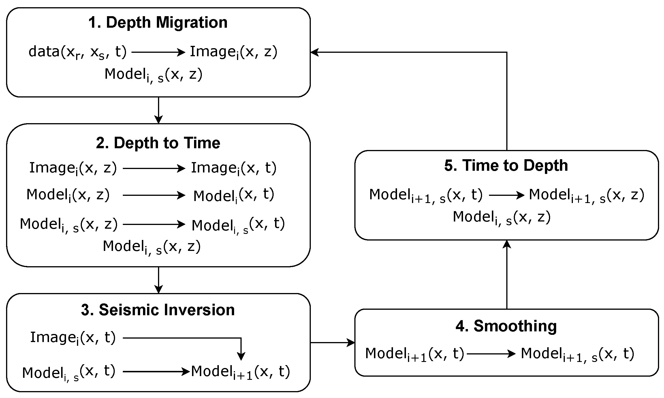
Figure 1, the first step of the joint algorithm is to obtain the seismic image in the depth domain.
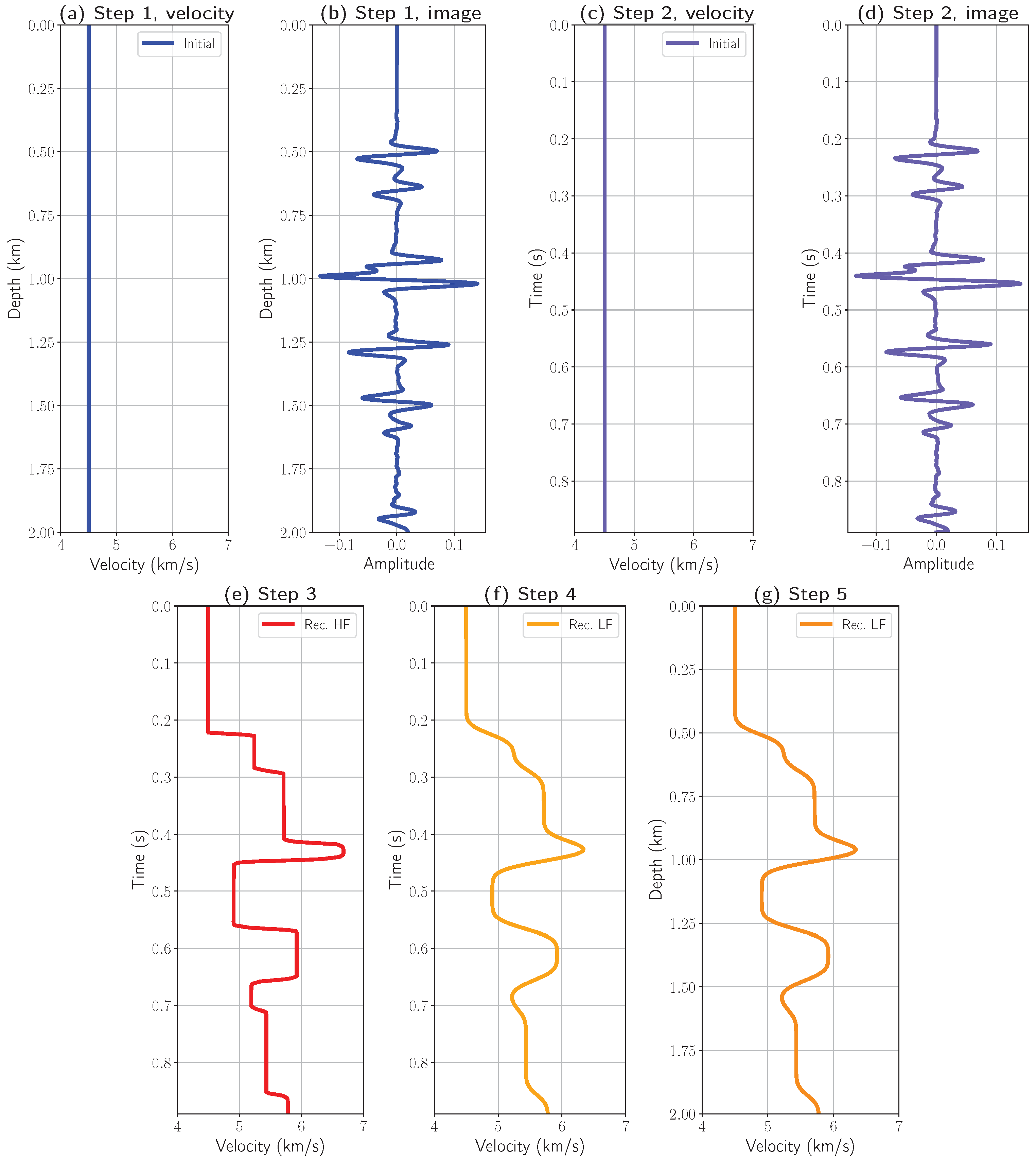
Figure 2a,b display the initial velocity model for depth migration and the resulting migrated seismic trace, respectively. The second step involves converting both the velocity model and the migration result to the time domain using the initial velocity from
Figure 2a. The transformed velocity model and seismic trace in the time domain are shown in
Figure 2c and
Figure 2d, respectively. The third step applies seismic inversion to reconstruct a detailed high-frequency model of the medium in the time domain (
Figure 2e). The fourth step extracts the low-frequency velocity component (
Figure 2f) from the time-domain inversion result. Finally, the fifth step converts the updated velocity model back to the depth domain, yielding the result shown in
Figure 2g. After completing these steps, we obtain an updated velocity model in the depth domain. In the next iteration, this updated velocity model is used in the depth migration algorithm and the “depth-to-time” transformation.
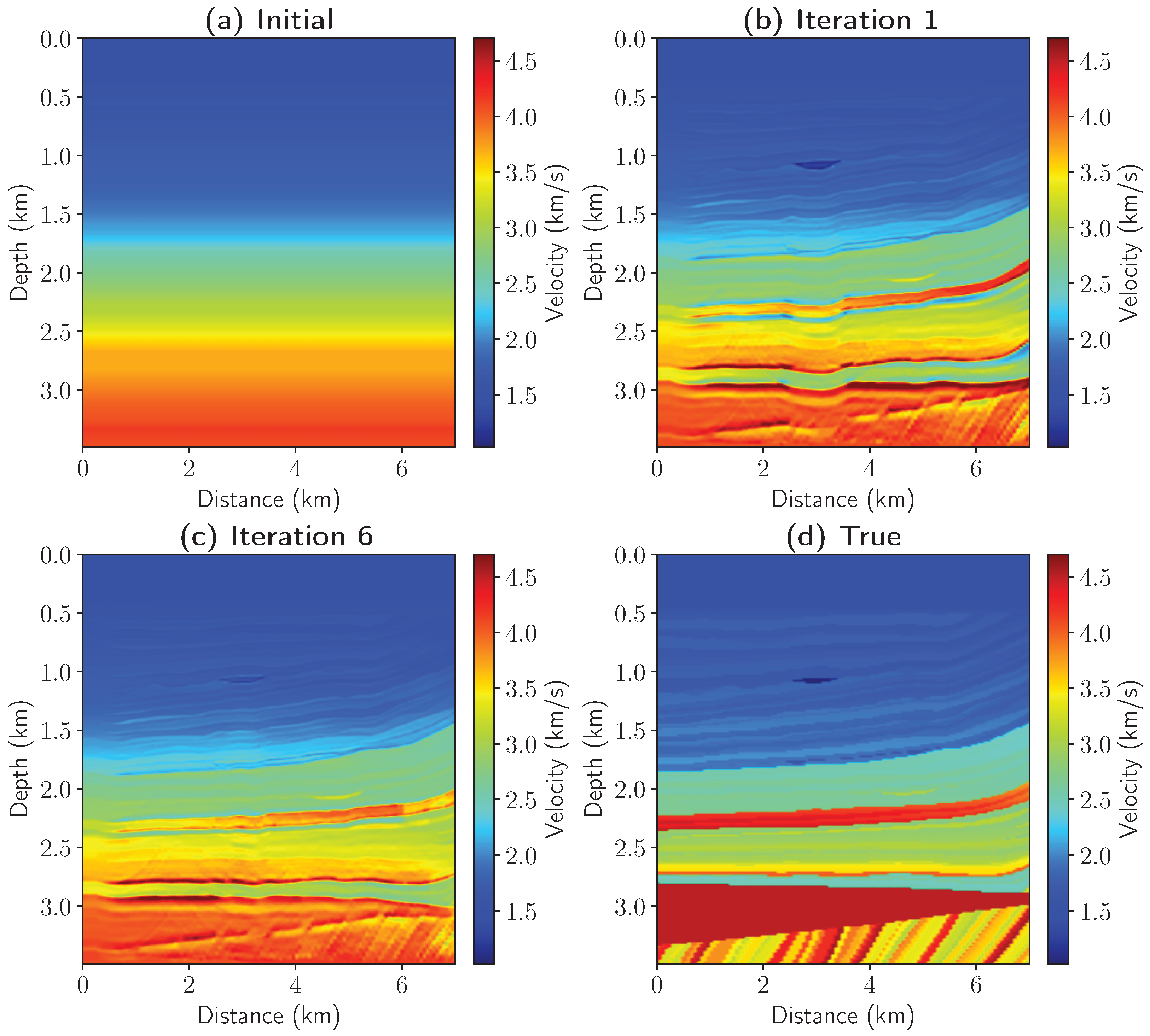
The proposed iterative algorithm is first applied to a realistic model from Eastern Siberia shown in
Figure 3d under the assumption that the density is constant also. A homogeneous model shown in
Figure 3a with values taken from the upper part of the true model was chosen as the initial model.
Figure 3b shows the layered velocity model produced by the first iteration of the joint algorithm. This model is qualitatively similar to the true velocity model, but the positions of the deeper boundaries were reconstructed inaccurately. After six iterations the joint algorithm converged to the model presented in
Figure 3c. Subsequently, increasing the number of iterations produces almost no change. Comparing the result of the joint algorithm to the true velocity model, it is evident that the positions of the boundaries and the velocity values were reconstructed with sufficient accuracy.
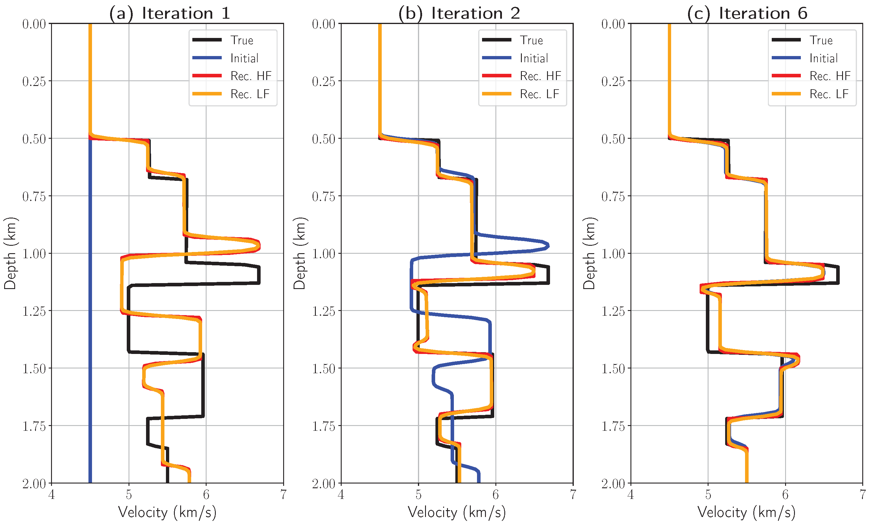
Figure 4 illustrates the iterative process for an individual trace. It can be observed that the layer boundaries converge to their true positions sequentially starting from the upper layers and progressing to the deeper ones even though the initial velocity model was far from accurate. However, one can observe velocity errors at the depths of 1.1 km and 1.5 km in
Figure 4c. The velocity changes significantly near high-contrast layers, which affects the seismic image and may cause the inversion to produce small artifact layers. We attribute the observed errors to these artifact layers generated during seismic inversion of high-contrast formations.
The objective function (
12) for the constrained total variation inversion consists of a residual norm and four regularization terms. The first two regularization terms ensure the sparsity of the reconstructed reflection coefficient trace. The third term integrates the initial impedance model into the inversion result. The final term enforces spatial continuity by incorporating inversion results from adjacent seismic traces. To demonstrate the contribution of each regularization term, we conduct the following numerical experiment.
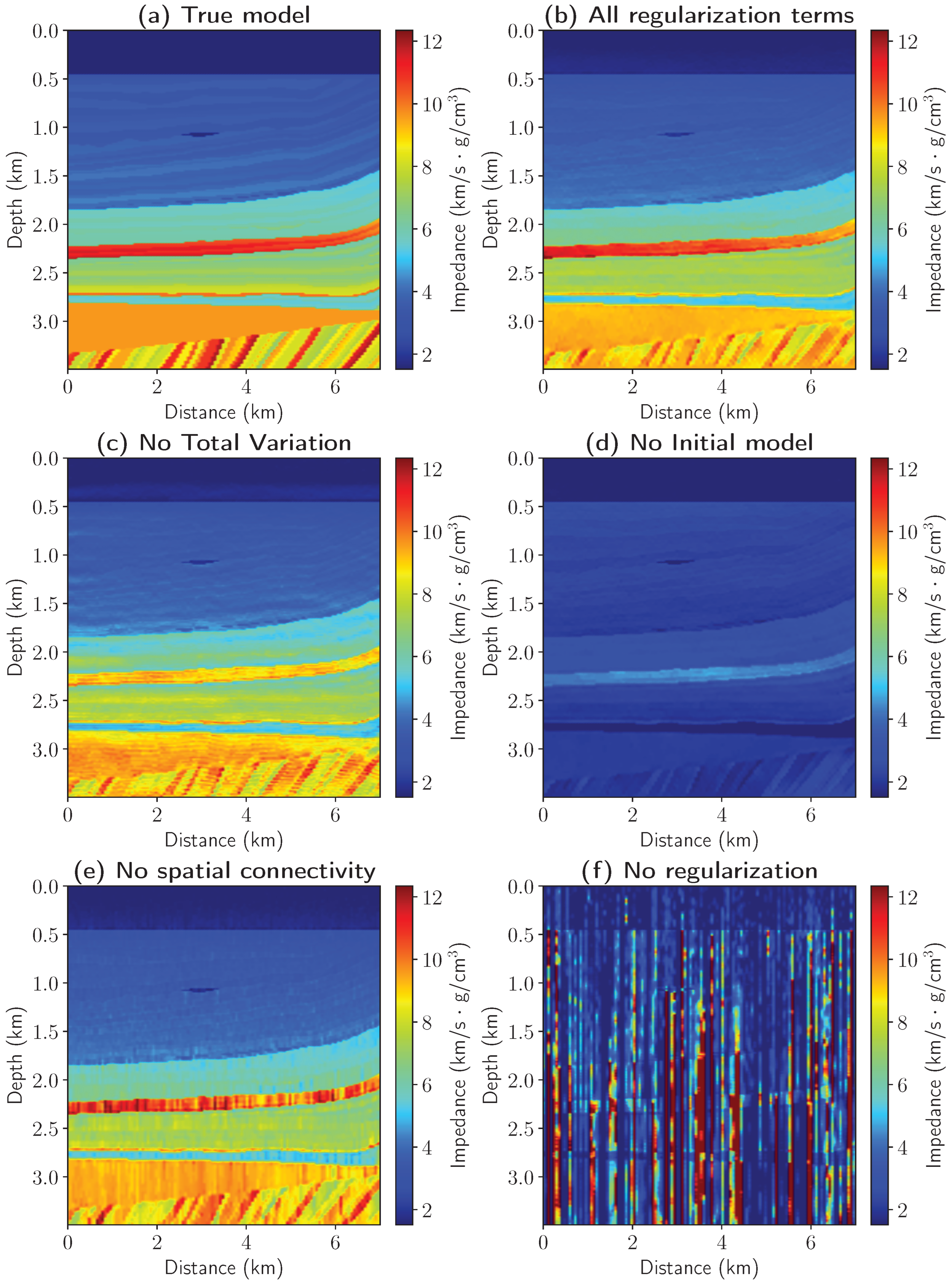
Figure 5a shows a section of the Marmousi model. We generate an ideal 1D convolution synthetic using this impedance model (via Equation (
1) with a Ricker wavelet), then add 20% Gaussian noise to create our input data for inversion. Using all four terms yields a highly detailed impedance model closely matching the true solution (
Figure 5b). Disabling the first two TV regularization terms produces an over-smoothed result with less focused impedance contrasts and blurred layer boundaries (
Figure 5c). When the initial model regularization term is disabled, the reconstructed model exhibits quantitative inaccuracies (
Figure 5d). When disabling the spatial term, vertical artifacts appear due to the 1D convolution assumption; the spatial term mitigates these by incorporating lateral trace information (
Figure 5e). Complete removal of regularization produces geologically implausible results with no resemblance to the true model (
Figure 5f). Each term in (
12) contributes to reconstructing a physically and geologically plausible impedance model by leveraging different prior information. Omitting any term introduces artifacts, demonstrating the necessity of comprehensive regularization in seismic inversion.
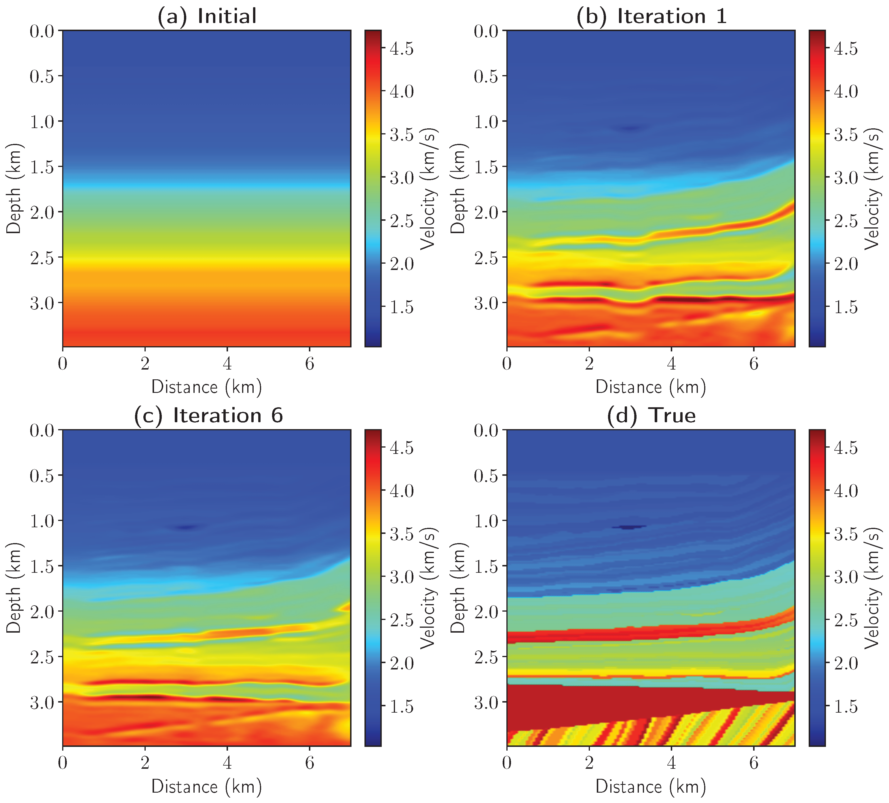
Figure 6 shows the results of applying the developed joint algorithm to a portion of the realistic Marmousi model again under the assumption that the density is constant and known. It should be noted that the rest of the Marmousi model is not considered here as the images produced by the simplified depth migration implementation are of insufficient quality for seismic inversion to be effectively applied, more sophisticated migration is necessary in this case. A horizontally layered smooth velocity model, shown in
Figure 6a, was chosen as the initial model for migration. In the first iteration of the joint algorithm seismic inversion produced the detailed velocity model shown in
Figure 6b. It is evident that the upper layers of the velocity model were updated more significantly while the deeper layers still required refinement. Subsequent iterations led to updates in the deeper layers and after six iterations the joint algorithm produced the velocity model shown in
Figure 6c; increasing iterations beyond six produce minimal effect. The reconstructed model is in good agreement with the true velocity model shown in
Figure 6d in terms of the structure and position of the layer boundaries. Comparing the initial velocity model with the model produced by the joint algorithm, it is clear that seismic inversion can be used as a means to reconstruct the macro-velocity model of the geologic medium in the depth domain.
The algorithm’s computational efficiency merits discussion. Depth migration represents the most computationally intensive component of the joint workflow. However, the joint migration–inversion algorithm typically converges within a few iterations. Our tests demonstrate convergence to a stationary point in fewer than ten iterations, with iterations beyond six yielding negligible model improvements.
Notably, the seismic inversion component accounts for only approximately 5% of total runtime. This marginal computational cost justifies employing more advanced (albeit slower) inversion algorithms to maximize information extraction from the depth migration results. For the 2D models presented here, the joint algorithm requires 1.5–2 h to converge on standard laptop hardware.
The presented results suggest that the joint algorithm of seismic inversion and depth migration is capable of refining the velocity model under the assumption that the density is constant and known. While this assumption is not practical in real-world scenarios the iterative process of seismic inversion and depth migration successfully extracts useful information about the macro-velocity model from the seismic data.
5.2. Elastic Model with Non-Constant Density
As demonstrated in the previous section, the iterative joint algorithm combining acoustic seismic inversion and depth migration can effectively refine the depth macro-velocity model of the medium without requiring overly strict initial conditions. Notably, the algorithm achieves convergence even when initialized with a velocity model substantially different from the true solution.
We now examine the case of an elastic model with a known but non-constant density distribution. For this scenario, we generate synthetic data using elastic finite-difference modeling. The workflow of the joint migration–inversion algorithm remains identical to the previous implementation. As before, we select a horizontally layered smooth velocity model as the initial input for migration.
When applying the joint algorithm to the Marmousi model, we obtain satisfactory results as presented in
Figure 7. Analysis of the left section reveals that the initial velocity model shown in
Figure 7a incorporates a relatively accurate low-frequency component of the true velocity model, enabling effective refinement through the joint algorithm. The smoothed velocity model after six iterations of the joint algorithm (
Figure 7c) shows excellent agreement with the true velocity model displayed in
Figure 7b.
Regarding the practical aspects of applying the joint algorithm, it is necessary to consider the case of unknown density, as this represents the most common real-world scenario. First, an initial acoustic impedance model is required to perform acoustic seismic inversion. Given a known initial velocity model, the initial acoustic impedance model can be derived using an empirical relationship between compressional wave velocity and medium density, such as Gardner’s equation. In model parts where these empirical relationships are valid, the derived acoustic impedance will closely match the true values, enabling accurate inversion.
After obtaining a detailed acoustic impedance model from inversion, a key challenge emerges: deriving an updated velocity model without known density. The proposed approach generates a smooth density model using empirical relationships from the previous smooth velocity model, then computes velocity by dividing the detailed impedance by this estimated density. Note that in this case, all impedance contrasts between consecutive layers will transfer to the velocity model, since the density model is smooth. It is expected that the iterative nature of the joint algorithm will help mitigate this limitation, prompting further numerical experiments.
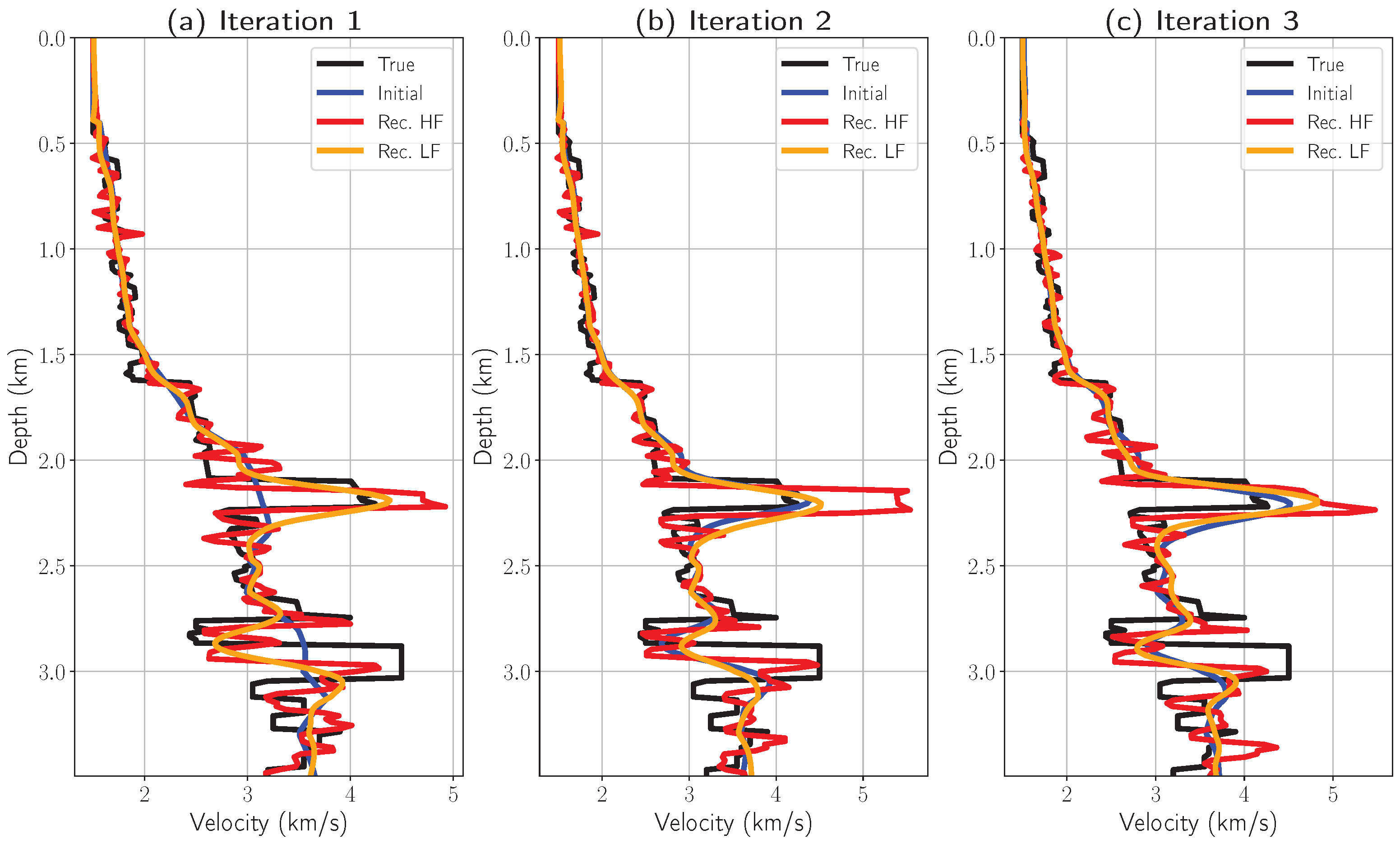
Consider a single trace from the Marmousi model.
Figure 8 illustrates the velocity model across three consecutive iterations of the joint algorithm. By comparing velocities at different iterations, it can be observed that the algorithm refines the velocity model during the first two iterations, but no further improvement is seen in the detailed velocity model afterward.
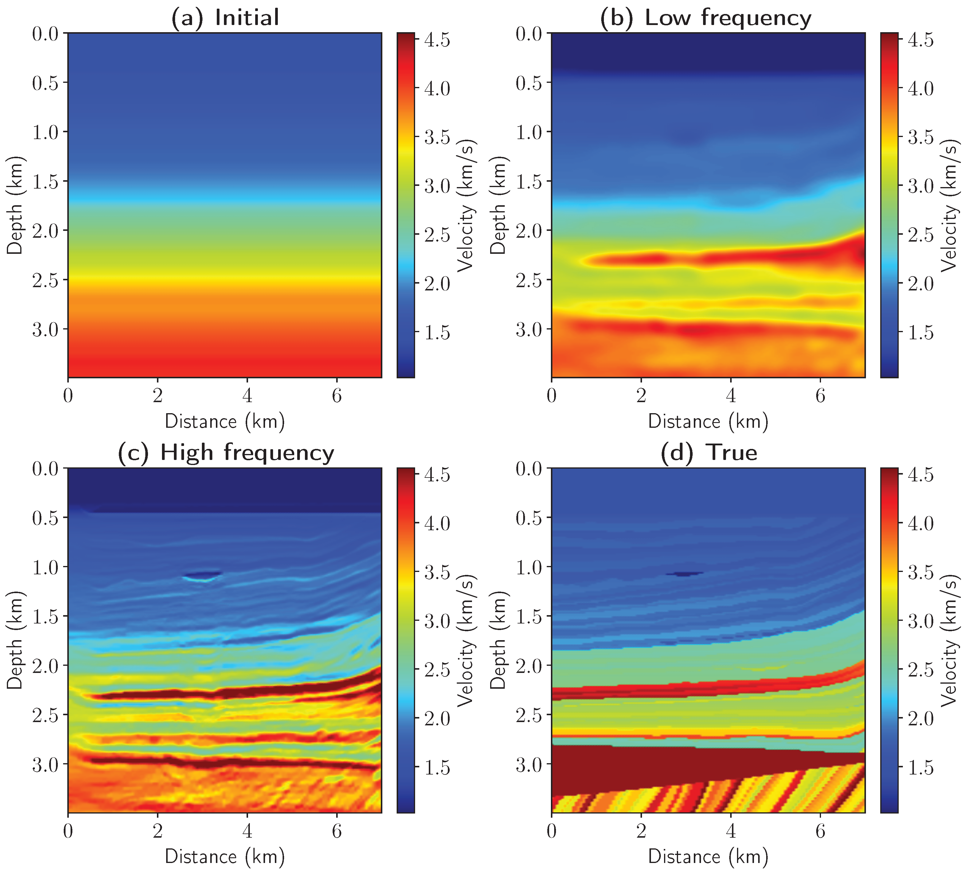
Although it is impractical to perform a large number of iterations of the proposed joint algorithm when density is non-constant and unknown, executing two iterations remains feasible, yielding refined high- and low-frequency/smooth depth velocity models. The reconstructed high-frequency velocity model after two iterations of the migration–inversion algorithm (shown in
Figure 9) displays notable similarities with the true velocity model. Additionally, this high-frequency velocity model provides a significant update compared to the initial model, effectively refining the smooth migration velocity model.
6. Discussion
We consider the acoustic case of the joint algorithm application, assuming a known density, and demonstrate its potential for reconstructing the macro-velocity model of the medium. In cases where density is unknown, an initial impedance estimate required for seismic inversion can be obtained using empirical relationships such as Gardner’s equation. Numerical experiments show, when density is non-constant and unknown, it is impractical to perform a large number of iterations of the proposed joint migration–inversion algorithm. Nevertheless, two iterations remain feasible, yielding refined high- and low-frequency depth velocity models. Further iterations are not viable because velocity and density cannot be separated using only the impedance model without additional a priori information.
Like any other approach, the presented method has certain limitations. Primarily, it inherits all the constraints of its constituent components—namely, acoustic seismic inversion and beam depth migration. For instance, since beam migration has limited resolution and acoustic seismic inversion similarly exhibits resolution constraints, the proposed method consequently shares these resolution limitations. To enhance resolution, one should employ the most advanced available techniques, such as sparse-layer inversion, reverse-time migration, or a combination of both. By replacing the constrained total-variation seismic inversion and beam depth migration in our proposed scheme, one can create new variants of iterative migration–inversion. These modified approaches warrant further investigation and may yield more practical solutions.
An additional challenge arises from the need to reconcile migration and inversion results—specifically, the connection between impedance and velocity. Consequently, the proposed algorithm requires supplementary density information. However, advanced elastic seismic inversion methods can recover both impedance and velocity models. Incorporating elastic inversion within the joint algorithm framework could help overcome this limitation and improve the method’s practical utility. In this study, we focus on acoustic inversion (normal incidence) using PP images only. For elastic inversion with multi-component data, PS images could be generated and utilized. Such data would enable joint PP-PS inversion, allowing reconstruction of both P-wave and S-wave velocity models. Furthermore, the method could be extended to anisotropic media by implementing anisotropic migration and anisotropic seismic inversion.
