Seasonal Sea Surface Temperatures from Mercenaria spp. During the Plio-Pleistocene: Oxygen Isotope Versus Clumped Isotope Paleothermometers

Abstract

The Mid-Piacenzian Warm Interval (MPWI) is marked by warmer temperatures and higher atmospheric CO₂ levels than today, making it an analogue for late-21st-century-warming, whereas the early Pleistocene cooling is more like today. We compare seasonal growth temperatures derived from oxygen isotope ratios (δ¹⁸O) and clumped isotopes (∆₄₇) in Mercenaria. Modern shells were previously collected from coastal NC. The fossil shells are from the Duplin (MPWI) and Waccamaw Formations (early Pleistocene), NC. Oxygen isotope ratios range from −2.2‰ to 2.3‰ (modern), −0.9‰ to 2.4‰ (MPWI), and −0.9‰ to 2.9‰ (early Pleistocene). The values of Δ₄₇ range from 0.576‰ to 0.639‰ (modern), 0.566‰ to 0.621‰ (MPWI), and 0.581‰ to 0.615‰ (early Pleistocene). We show that Mercenaria do not require a species-specific ∆₄₇ calibration. Modern and MPWI ∆₄₇-derived summer/winter temperatures (SST_∆47) and seasonal amplitudes are indistinguishable from δ¹⁸O-derived temperatures. The early Pleistocene summer SST_∆47 is indistinguishable from δ¹⁸O-derived temperatures, but the winter SST_∆47 is warmer by 5 °C and may reflect within-shell time averaging. The modern summer/winter SST_∆47 are indistinguishable from the MPWI, but the MPWI has a lower seasonal amplitude by 5 °C. Compared to our calculated δ¹⁸O_sw values, modeled values for the MPWI are within error but are much lower, and they are not within error for the early Pleistocene.

1. Introduction

Seasonal-scale climate reconstructions of recent warm intervals are more relevant than ever to understanding the consequences of the warming climate of today and into the future; however, most reconstructions and model outputs focus on global and annual scales [1,2,3,4]. The 2021 report by the Intergovernmental Panel on Climate Change (IPCC) projects a mean annual global warming of ~3–5 °C by 2100 following the moderate Shared Socioeconomic Pathway (SSP) 2–4.5 [5]. The 1990 IPCC report estimated that by 2030 mean global temperatures would increase by 0.7–1.5 °C, with a best estimate of 1.1 °C [6]. The mean annual temperature in 1990 was 11.9 °C, and in 2023 it was 13.1 °C [7] already surpassing the 1990 IPCC report’s best estimate. The 2007 IPCC report identified the mid-Pliocene (now known as the Mid-Piacenzian Warm Interval; MPWI) as an analogue for future global warming due to its warmer temperatures and higher atmospheric CO₂ levels than today [8]. The higher CO₂ levels are similar to Representative Concentration Pathways (RCPs) 4.5 and 8.5 [9,10]. The RCPs are projections of greenhouse gases and their impact on climate by 2100 [11]. Subsequent cooling during the early Pleistocene resulted in temperatures and pCO₂ values more similar to today [12].

Shallow and nearshore bioarchives offer particularly valuable records of regional climate, hydrologic cycles [13], and land–sea interactions [14], while also resolving seasonal thermal variability [15,16,17,18,19,20]. Bioarchives like bivalve shells record the temperature at which growth occurs and, therefore, may not always represent mean sea surface temperature (SST) [21]. As growth rates are not constant year-round, mean annual temperatures will be biased towards the season in which the most growth occurs [22]. Most biocarchives found in cold-temperate zones grow during the warmest parts of the year, while those in warm-temperate zones grow during the colder parts of the year [19]. To capture seasonal variability, bioarchives must grow at fast enough rates to achieve subseasonal/submonthly resolution. Shells from the hard clam genus Mercenaria have long been recognized as a rich archive of seasonal variability in modern, archeological, and deep-time contexts, especially early in ontogeny when growth rates are fast and make fortnightly resolution possible (Figure 1) [19,23,24]. The typical growth rates of Mercenaria from North Carolina are ~12 mm/year [25]. Mercenaria occurs in the fossil record extending to the Oligocene [26,27] and are commonly found in sedimentary rocks that preserve climate intervals of interest such as the MPWI and early Pleistocene. Oxygen isotope ratios (δ¹⁸O) preserved in carbonate biominerals of marine organisms such as bivalves, corals, and foraminifera are widely used to reconstruct SST during periods of skeletal growth [23,28,29]. Traditional δ¹⁸O proxies commonly used in shallow-marine/estuarine biogenic archives to reconstruct deep-time climate change can be complicated by the assumptions of δ¹⁸O seawater (δ¹⁸O_sw) values. Paleoclimate reconstructions require assumptions about the ambient δ¹⁸O_sw value at the time the hard part remains were formed. Such assumptions can lead to discrepancies in water temperature estimates and seasonal variation. The development of the clumped isotope (∆₄₇) paleothermometer avoids this problem as it is an independent paleotemperature proxy and does not rely on constraining the δ¹⁸O_sw value [30,31]. In combination, the δ¹⁸O and ∆₄₇ proxies can be used to calculated the δ¹⁸O_sw value during the time of shell formation and assess previous δ¹⁸O_sw assumptions based on ice volume models [32].

This study compares reconstructed seasonal-scale SST based on clumped isotope geochemistry versus oxygen isotope ratios between modern and Plio-Pleistocene bivalve shells. We compare these proxies in modern Mercenaria shells from the Mid-Atlantic Coastal Plain (MACP) and then apply the clumped isotope proxy as a paleothermometer in shells from the MPWI and subsequent early Pleistocene cooling from Mercenaria fossils at seasonal resolution. Fossil shells were collected from the Duplin and Waccamaw Formations in North Carolina within the MACP. Modern specimens were collected off the North Carolina coast at approximately the same latitude. We tested the following hypotheses: (1) Mercenaria do not require a species-specific clumped isotope calibration; (2) ∆₄₇-derived SST (SST_Δ47) values are similar to δ¹⁸O-derived temperatures; (3) SST_Δ47-derived δ¹⁸O_sw values are indistinguishable from those derived from previously published methods using the δ¹⁸O_sw–salinity relationship; (4) Mercenaria shells from the MPWI record warmer summers and winters compared to the early Pleistocene and today; (5) shells from the MPWI record reduced seasonality compared to those from the early Pleistocene and today.

2. Geologic Context

2.1. Pliocene Formations (Duplin/Yorktown)

The US Mid-Atlantic Coastal Plain (MACP; 34° N to 38° N) extends north from the northeastern edge of South Carolina and Georgia to southern New Jersey. This region is crucial for paleoclimate studies as it includes two distinct marine biogeographic zones: warm-temperate and cold-temperate [20,33]. According to Briggs and Bowen (2012) [33], the cold-temperate zone stretches from Cape Hatteras, North Carolina, to the Strait of Belle Isle between Newfoundland and Labrador, while the warm-temperate zone extends from Cape Canaveral, Florida, to Cape Hatteras. Briggs and Bowen (2012) [33] define the modern dividing line between these zones near Cape Hatteras (Figure 2). Thus, sedimentary deposits within the MACP, such as in North Carolina, may reflect historical shifts in the boundary between the warm- and cold-temperate zones.

The Plio-Pleistocene stratigraphy of the MACP has been extensively researched [36,37,38]. From Florida to Virginia, outcrops are visible, but they dip below the surface north of Maryland. In Virginia, the Pliocene Yorktown Formation is divided into four members: Sunken Meadow, Rushmere, Morgarts Beach, and Moore House. These members correspond to three distinct transgressive events separated by unconformities, with the Rushmere and Morgarts Beach Members marking a single transgression [38]. The fossilized molluscs and microfossils found in the Yorktown Formation indicate it was deposited in offshore, fully marine settings [16,17,36,38,39,40,41,42]. Similarly, the Pliocene Duplin Formation in the Carolinas was deposited during the same transgressions that resulted in the Rushmere, Morgarts Beach, and Moore House Members of the Yorktown Formation [43,44,45], covering the southern part of the MACP (see Figure 2 in [35]). Earlier studies estimated that sea level during the Middle Pliocene Warm Interval (MPWI) was ~35 ± 18 m higher than it is today [42], similar to estimates for the Yorktown Formation (20–30 m; [16]). However, recent studies suggest a maximum sea level rise of 25 m [46,47].

According to Blackwelder (1981) [37] and Ward et al. (1991) [17], the Yorktown and Duplin Formations feature marine fauna typical of warm-temperate conditions, with some tropical species also present. The absolute age of the Yorktown Formation has not been precisely determined using geochronologic dating methods, but micropaleontological evidence places its deposition between 4.0 and 2.9 million years ago [48]. Krantz (1991) [38] proposed that the deepest transgression within the Yorktown Formation, reflected in the Rushmere and Morgarts Beach Members (30–40 m depth), occurred during the peak warmth of the mid-Pliocene. Ward et al. (1991) [17] estimated the timing of this event to be around 3.4 to 3.0 million years ago based on molluscan assemblages. More recently, Dowsett et al. (2021) [49] linked the Rushmere Member to the latter part of the Marine Isotope Stage (MIS) M2-M1 transition and the Morgarts Beach Member to MIS KM5-KM3, correlating these members to approximately 3.3–3.0 million years ago. Williams et al. (2009) [45] bracketed the Duplin Formation to between 3.8 and 3.4 million years ago, though the exact range varies across different studies (see [42] and references therein).

2.2. Pleistocene Formations (Waccamaw/Chowan River)

In the MACP, the early-Pleistocene Gelasian-aged Chowan River Formation in Virginia unconformably overlies the Pliocene (late Zanclean and early Piacenzian) Yorktown Formation [38]. The correlative Bear Bluff and Waccamaw Formations in North Carolina also occur in the early Pleistocene but are less extensive than the Chowan River Formation, likely reflecting a shallower paleodepth of around 15 m [38]. These formations were deposited during a transgressive event under cooler global conditions compared to the mid-Piacenzian warmth during the deposition of Yorktown and Duplin Formations [40,50]. Biostratigraphy in the Waccamaw Formation indicates an age of approximately 1.8 to 2.1 million years, representing less than a million years of deposition [36,43,51]. Gibbard et al. (2010) [52] redefined the Gelasian stage as part of the Pleistocene rather than the Pliocene. Although our study does not include specimens from the Chowan River Formation, we mention it here for context and comparison, given its extensive evaluation compared to the Waccamaw/Bear Bluff Formations in North Carolina. Several researchers have classified the Chowan River Formation as warm-temperate [16,17,41]. However, isotopic data suggests winter temperatures below 12 °C [16,20,35], indicating cold-temperate conditions as defined by Briggs (1995) [52] and Briggs and Bowen (2012) [32]. While Blackwelder (1981) [37] described mollusc assemblages from the Waccamaw Formation as indicative of warm-temperate conditions, there is currently one quantitative sea surface temperature (SST) reconstructions for this formation [35].

2.3. Mercenaria Ecology

The genus Mercenaria first appears in fossil deposits along the MACP during the Oligocene [25,26] and ranges from southern Florida to southern New Jersey along the Atlantic and Gulf of Mexico coasts of the United States [53,54,55]. Currently, two species of Mercenaria are found within the MACP: M. mercenaria (the northern hard clam) and M. campechiensis (the southern hard clam). M. mercenaria is particularly important to the U.S. shellfish industry, contributing over 6 million pounds of shellfish and generating USD 51 million in revenue annually [56]

The genus Mercenaria inhabits a variety of environments, ranging from estuarine to shallow-marine and from intertidal to subtidal zones [57]. They grow in water temperatures between 9 and 31 °C, with the fastest growth occurring between 15 and 25 °C [24]. Salinity also affects their growth rates, which slow when salinity drops below 17 psu [58]. Mercenaria are a long-lived bivalve species, living up to 40 years old [59]. Their growth rate is most rapid during the first five to six years of life [59], and other factors like food availability, quality, and reproduction can also influence growth [60,61].

Mercenaria shells are composed of three aragonitic layers. The outer layer contains prismatic aragonitic units and sometimes crossed-lamellar and columnar prismatic microstructures [62]. The middle and inner layers are made up of complex cross-lamellar structures, termed “homogeneous” due to their indistinguishable, non-repeating small structural units [62,63,64]. Growth patterns are visible in the outer and middle layers but are most apparent in the middle layer, characterized by alternating dark (transparent) and light (opaque) increments under reflected (transmitted) light [62]. Dark increments form during periods of slow growth, typically when temperatures fall below or rise above their respective thresholds [65,66]. There is a documented relationship between the formation of dark growth increments and latitude. For example, Mercenaria collected north of Virginia form dark increments in winter when temperatures drop below 10 °C for extended periods [60,67]. In contrast, those from lower latitudes (i.e., South Carolina, Georgia, and Florida) form dark increments during summer when temperatures exceed 25 °C [23,68,69]. This pattern is also seen in limpet shells from the eastern North Atlantic [70]. However, this pattern can be more complex at higher mid-latitudes. Henry and Cerrato (2007) [71] found that Mercenaria shells collected over two decades initially formed dark increments in winter, but later specimens showed increments forming in summer or in both seasons, possibly due to anthropogenic changes in the watershed. Elliot et al. (2003) [72] observed that Mercenaria shells from Cedar Key, Florida to Oyster Bay, New York, showed slowed growth during summer. By examining the ontogenetic age of the shell and the location of dark increment formation relative to oxygen isotope timeseries, the timing of seasonal changes in growth rates and growth temperature variability can be determined [18,73].

3. Methods

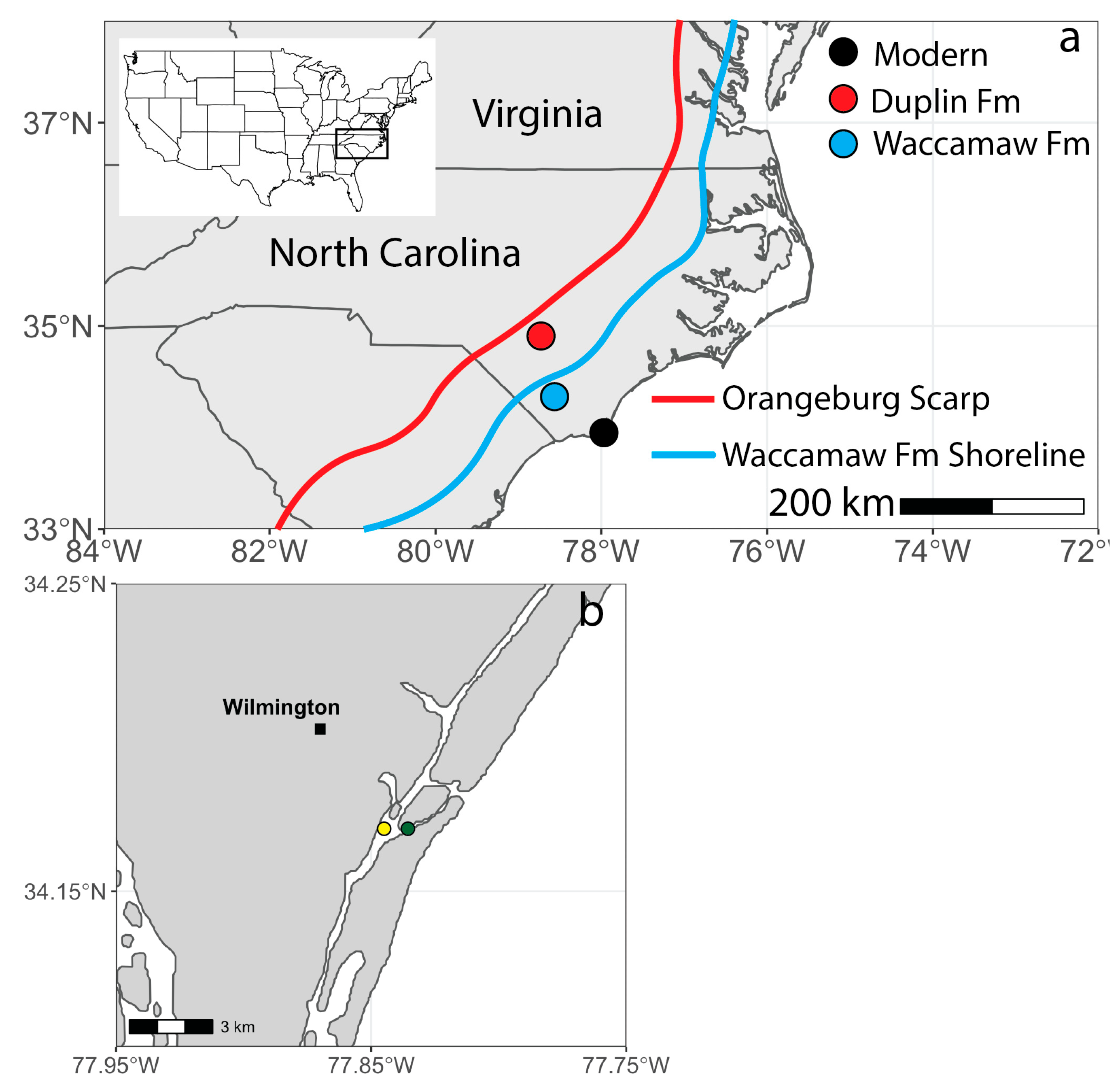
3.1. Modern and Fossil Shell Collection

Modern M. mercenaria shells (n = 39) were collected alive on 29 April 2019 at ~1 m depth from the University of North Carolina at Wilmington’s (UNCW) Marine Sanctuary (NC-SANC; Figure 2) and were used in an earlier life history study [74]. Four shells were selected from Palmer et al. (2021) [74] based on physical shell condition (i.e., no cracks or broken shell material after shell processing) across a range of ontogenetic ages to maximize unique years of shell growth (i.e., non-overlapping years of growth across individual specimens). Shells ranged in age from 5 to 15 years old based on the annual couplets of dark and light increments [74].

Water quality data (temperature and salinity) were accessed through the NOAA’s National Estuarine Research Reserve System (NERRS) database (https://cdmo.baruch.sc.edu/dges/) accessed on 1 April 2021. We obtained water monitoring data from the NERRS station Loosin Creek (site #NOCLCWQ) (Figure 2). This monitoring station is 1.2 km away from the shell collection locality. A YSI EXO2 multiparameter water quality sonde at this station records temperature and salinity measurements every 30 min beginning on 26 February 2002 and every 15 min after 21 August 2006 with a precision of ±0.01 °C and ±0.01.

Assumptions regarding time averaging within stratigraphic units must be considered when utilizing fossil specimens. Kidwell (1998) [75] describes uncertainties that can exist and strategies that can be implemented to decrease uncertainty associated with time averaging. Braniecki et al. (2024) [35] go into more detail regarding the time averaging associated with the Duplin and Waccamaw Formations, and readers are directed to that publication. Briefly, we assumed that our fossil shell localities represent the “within-habitat” time-averaged category and, therefore, similar environmental conditions throughout. Duplin Formation shells were collected from the Robeson Farm locality southwest of the Cape Fear River, approximately 2 km east-southeast of Tar Heel, North Carolina. Shells from the Lower Waccamaw Formation (early Pleistocene) were collected from the Register Quarry locality in Columbus County, North Carolina. For further details regarding the collection sites, see Palmer et al. (2021) [74]. Two shells were selected for isotopic analysis from each formation for a total of four fossil shells. They were selected based on taphonomic and diagenetic assessments as described below.

3.2. Taphonomic and Diagenetic Assessments and Shell Preparation

We selected fossil shells used in the earlier study by Palmer et al. (2021) [74]. Fossil specimens were tested for diagenetic alteration of aragonite to calcite using X-Ray Diffraction (XRD) at the University of North Carolina’s (UNC) Chapel Hill Analytical and Nanofabrication Laboratory (CHANL), which showed that the shells maintained their original mineralogical composition. For more details regarding XRD analysis, see Braniecki et al. (2024) [35]. Shell thick sections were previously processed by Palmer et al. (2021) [72], who avoided shells with cracks, bore holes, or other taphonomic damages. Shell cross-sections were imaged using an Olympus SZX7 stereomicroscope and did not show visual evidence of secondary mineralization or modification.

3.3. Micromilling and Isotopic Analysis

Three years of shell growth between ontogenetic years 2 and 5 were targeted for micromilling. We did not sample ontogenetic year one because the curvature of the growth increments was difficult to digitize. Ontogenetic year two in the shells NC_SANC_23 and NC_SANC_27 was avoided for the same reason as ontogenetic year one. We collected ~50 μg of carbonate powder per microsample. For more details regarding the micromilling process, see Braniecki et al. (2024) [35]. Oxygen isotope ratios of shell carbonate were determined on a Finnigan MAT 252 mass spectrometer with an auto-carbonate reaction system (Kiel III Device) at the Environmental Isotope Laboratory at the University of Arizona. Powdered samples were reacted with dehydrated phosphoric acid under vacuum at 70 °C. The isotope ratio measurement was calibrated based on repeated measurements of NBS-19 and NBS-18 standards. Precision was ±0.11‰ for δ¹⁸O and ±0.08‰ for δ¹³C (1σ), based on repeated measurement of internal standards. Results are reported in per mil units (‰) relative to the VPDB (Vienna Pee Dee Belemnite) standard.

We targeted the local maxima and minima in the δ¹⁸O_shell timeseries for carbonate clumped isotope (Δ₄₇) samples to maximize the range in temperatures. We collected ~2.5 mg of carbonate powder using a NSK V-max Volvere handheld dental drill with a Brasseler USA Dental Rotary Instruments tungsten carbide round-head drill bit (catalog number H71.11.008). These carbonate powders were analyzed for clumped (Δ₄₇) and stable (δ¹⁸O, δ¹³C) isotopes in the Paleo³ Isotope Lab at North Carolina State University (NCSU). Analyses at NCSU were carried out on a Nu Perspective IS Mass Spectrometer with a NuCarb Autosampler. Samples and standards (~500 µg) were digested at 70 °C with orthophosphoric acid in a NuCarb automated carbonate device and the CO₂ released from the reaction was cryogenically purified using a series of cold fingers and a Porapak Q trap at −28 °C. Purified CO₂ was passed via a dual inlet into a Nu Perspective IS Mass Spectrometer, which was set to measure m/z ratios for masses 44 to 49. Samples were analyzed using solid standards calibrated versus Vienna Peedee Belemnite (VPDB) for δ¹⁸O and δ¹³C, and the Intercarb-Carbon Dioxide Equilibrium Scale (I-CDES) for Δ₄₇ [76]. Carbonate standards were analyzed using the same procedure utilized on sample replicates and were included in every run. The carbonate standards used included international standards NBS-18, ETH-1, ETH-2, ETH-3, ETH-4 (c.f., [76]), and internal standards Merck, C1, C2, and C64. Data was reduced using Easotope [77] and pooled standardization approaches [78], and temperatures were calculated using the method of Anderson et al. (2021) [79], with Brand et al. (2010) [80] ¹⁷O correction parameters. The long-term precision was ±0.15‰ for δ¹⁸O, ±0.1‰ for δ¹³C, and ±0.015‰ for Δ₄₇ (SE) based on repeated measurements of standards.

3.4. δ¹⁸O-Derived Temperature Calculations

The relationship between δ¹⁸O_shell values and temperature is well studied (e.g., [81,82,83,84]). These studies have defined relationships between temperature, δ¹⁸O_shell, and δ¹⁸O_w values. We used the following salinity–δ¹⁸O_w relationship published by Elliot et al. (2003) [71] to estimate δ¹⁸O_w values:

δ¹⁸O_w = 0.17S − 5.19

(1)

where S is salinity. Braniecki et al. (2024) [35] provide more details about the rationale for using this equation. To estimate expected δ¹⁸O_shell values, we used daily temperatures measured at the Loosin Creek water monitoring station (<1.5 km away from shell collection site) and the following equilibrium fractionation equation for aragonite (Dettman et al., 1999 [84] modified from Grossman and Ku, 1986 [84]):

1000 ln α = 2.559 (10⁶ × T⁻²) + 0.717

(2)

where T is the temperature in Kelvin and α is the fractionation factor between water and aragonite, described by the following equation:

$$\mathsf{\alpha }{\displaystyle \frac{\mathrm{a}\mathrm{r}\mathrm{a}\mathrm{g}\mathrm{o}\mathrm{n}\mathrm{i}\mathrm{t}\mathrm{e}}{\mathrm{w}\mathrm{a}\mathrm{t}\mathrm{e}\mathrm{r}}}={\displaystyle \frac{(1000+{\mathsf{\delta }}^{18}{\mathrm{O}}_{\mathrm{a}\mathrm{r}\mathrm{a}\mathrm{g}\mathrm{o}\mathrm{n}\mathrm{i}\mathrm{t}\mathrm{e}\left(\mathrm{V}\mathrm{S}\mathrm{M}\mathrm{O}\mathrm{W}\right)})}{(1000+{\mathsf{\delta }}^{18}{\mathrm{O}}_{\mathrm{w}\mathrm{a}\mathrm{t}\mathrm{e}\mathrm{r}\left(\mathrm{V}\mathrm{S}\mathrm{M}\mathrm{O}\mathrm{W}\right)})}}$$

(3)

Values of δ¹⁸O_aragonite are relative to Vienna Standard Mean Ocean Water (VSMOW); therefore, they must be converted to Vienna Pee Dee Belemnite (VPDB) using the following equation from Gonfiantini et al. (1995) [85]:

δ¹⁸O_aragonite (VSMOW) = 1.03091 (1000 + δ¹⁸O_aragonite (VPDB)) − 1000

(4)

We used a δ¹⁸O_w value of 1.1‰ for the Duplin Formation, as published by Williams et al. (2009) [45]. A δ¹⁸O_w value of 0.0‰ was used for the Waccamaw Formation following Krantz (1990) [16] and Winkelstern et al. (2013) [19]. We assumed that the δ¹⁸O_w value remained constant throughout the year for each time interval.

3.5. Age Model

To match the δ¹⁸O_shell timeseries recorded by our modern Mercenaria shells, age models were constructed using a well-established “wiggle matching” technique to assign dates to our measured δ¹⁸O_shell values [86,87,88]. This technique uses local maxima and minima in the δ¹⁸O-derived temperature timeseries and maxima and minima in recorded temperature as tie points. The remaining measured δ¹⁸O-derived temperatures between the tie points were matched with similar temperature values to minimize errors associated with assuming continuous growth throughout the year [87]. The collection date, 29 April 2019, anchors the date of last shell growth. Counting annual light and dark growth increments back in time from the collection date provided the calendar years assigned to micromilled paths within the shells.

3.6. δ¹⁸O_sw Calculations

Seawater oxygen isotope ratios (δ¹⁸O_sw) were estimated from measured carbonate δ¹⁸O_shell values and temperatures reconstructed from SST_Δ47 using the following procedure: Step 1: The fractionation factor, α, was calculated using Equation (1) and SST_Δ47. Step 2: α and the δ¹⁸O_shell-VSMOW value, measured simultaneously with the Δ₄₇ value, were used to calculate δ¹⁸O_sw using Equation (2). To propagate uncertainties in the δ¹⁸O_sw estimates which consider errors in temperature and δ¹⁸O_shell, we used the following quadratic equation:

$$S{E}_{\left\{{\delta }^{18}{O}_{sw}\right\}}=\sqrt{\left\{{\left.\left({\delta }^{18}{O}_{sw}-{{\delta }^{18}{O}_{sw}}^{(T+{SE}_T)}\right.\right)}^2+{\left.\left({\delta }^{18}{O}_{sw}-{{\delta }^{18}{O}_{sw}}^{({\delta }^{18}{O}_{shell}+{SE}_{{\delta }^{18}{O}_{shell}})}\right.\right)}^2\right\}}$$

(5)

where SE_T is the standard error in temperature and SE_δ¹⁸_Oshell is the standard error in the carbonate δ¹⁸O value. The impact of temperature uncertainty on δ¹⁸O_sw was assessed by recomputing the equation with (T + SE_T), while δ¹⁸O_shell uncertainty was propagated by recalculating with δ¹⁸O_shell + SE_δ¹⁸_Oshell. Values of δ¹⁸O_sw and associated uncertainties were computed for each sample. The overall mean was calculated as a weighted mean, with weights based on the inverse variance of individual δ¹⁸O_sw estimates. The standard error (SE) of the weighted mean was derived from

$$S{E}_{mean}=\sqrt{{\displaystyle \frac{1}{\mathsf{\Sigma }1/{SE}_{{\mathsf{\delta }}^{18}\mathrm{O}\mathrm{s}\mathrm{w}}^2}}}+0.29\mathrm{‰}$$

(6)

The additive 0.29‰ term reflects the natural variation in the δ¹⁸O_sw values during the periods of growth for the shells.

3.7. Bootstrap Analysis

To evaluate the differences between the small, reconstructed datasets (e.g., SST_Δ47 or δ¹⁸O_sw estimates) and larger datasets (e.g., instrumental records or salinity-derived δ¹⁸O_sw), we implemented a weighted bootstrap procedure tailored to the unique uncertainties of each data type. Reconstructed SST_Δ47 values were accompanied by propagated SEs that incorporated analytical precision and the root mean squared error (RMSE) of the Anderson et al. (2021) [79] clumped isotope calibration. For δ¹⁸O_sw values derived from salinity, uncertainty was represented by the RMSE of the regional δ¹⁸O_sw–salinity regression, which accounts for calculated residuals and unmeasured environmental variation. Reconstructed δ¹⁸O_sw values based on SST_Δ47 and measured δ¹⁸O_shell values were assigned propagated errors based on uncertainties in temperature and δ¹⁸O_shell.

Weighted means and SEs were calculated using inverse-variance weighting to reflect the relative confidence of each data point. To assess statistical significance between groups, we used a Monte Carlo bootstrap approach. Each iteration (n = 10,000) drew a value from a normal distribution defined by the reconstructed mean and its SE, and a second value from a normal distribution centered on the calculated mean and either the RMSE (if derived from linear regression) or SE (if empirical, i.e., from measured data) of the large dataset. The difference between these draws was recorded, and a 95% confidence interval (CI) for the difference in means was derived from the resulting distribution. If the 95% CI contained 0, then the datasets were indistinguishable.

This approach allows for a direct comparison of datasets that differ substantially in size and uncertainty structure. By explicitly incorporating propagated errors from analytical measurements and calibration equations, the bootstrap method provides a realistic assessment of statistical difference without relying on assumptions of equal variance or normality. This method was applied consistently across modern and fossil datasets in this study to evaluate the fidelity of clumped isotope reconstructions.

4. Results

The following results encompass three types of isotopic data: δ¹⁸O of shell carbonate, analyzed as a timeseries on a conventional Finnigan IRMS, and targeted samples at peaks and valleys along the timeseries for paired δ¹⁸O and Δ₄₇ values, analyzed on a Nu IRMS. We will distinguish between the two types of δ¹⁸O data by referring to them as either timeseries or targeted.

4.1. Isotopic Compositions of Modern Shells

Modern shells exhibit the expected quasi-sinusoidal variation in the δ¹⁸O_shell timeseries. The combined δ¹⁸O_shell timeseries (i.e., among all modern shells) range from 2.3‰ to −2.2‰, with summer averages between −1.6 ± 0.5‰ and −1.3 ± 0.6‰ and winter averages between 0.8 ± 0.6‰ and 1.1 ± 0.7‰ (Figure 3). The lowest values coincide with dark increment formation. Shell growth is fastest during the transition from high to low δ¹⁸O_shell values and slowest from low to high values. The oxygen isotope timeseries from four modern shells record 11 unique seasonal cycles. Targeted δ¹⁸O_shell values along the peaks and valleys of the timeseries range from −2.1‰ to 1.4‰, with winter averaging 0.9 ± 0.3‰ and summer averaging −1.6 ± 0.6‰. The reduced seasonal amplitude of targeted δ¹⁸O_shell values compared to the δ¹⁸O_shell timeseries is likely due to the large sample size requirements needed for Δ₄₇ analysis. Clumped isotope values range from 0.576‰ to 0.639‰, with winter averaging 0.626 ± 0.008‰ and summer averaging 0.527 ± 0.185‰ (Figure 3 and

Table 1. Average summer and winter isotopic results from targeted clumped isotope sampling. All errors represent SE.

Age/Formation/Location	Shell ID	Season	δ18O VPDB	Δ47 ICDES	Temperature (Δ47)
Modern
North Carolina	NC_SANC_21	Summer	−1.7 ± 0.4‰	0.586 ± 0.003‰	28 ± 1 °C
		Winter	0.9 ± 0.5‰	0.626 ± 0.011‰	15 ± 3 °C
North Carolina	NC_SANC_24	Summer	−1.9 ± 0.1‰	0.588 ± 0.008‰	27 ± 3 °C
		Winter	0.9 ± 0.2‰	0.626 ± 0.009‰	15 ± 3 °C
North Carolina	NC_SANC_27	Summer	−1.7 ± 0.3‰	0.581 ± 0.005‰	29 ± 2 °C
		Winter	1.0 ± 0.2‰	0.625 ± 0.005‰	15 ± 1 °C
Mid-Piacenzian
Duplin Fm, NC	DUP-13	Summer	−0.5 ± 0.2‰	0.582 ± 0.014‰	29 ± 5 °C
		Winter	0.7 ± 0.6‰	0.615 ± 0.005‰	18 ± 2 °C
Duplin Fm, NC	DUP-24	Summer	−0.0 ± 0.3‰	0.577 ± 0.008‰	31 ± 3 °C
		Winter	0.3 ± 0.1‰	0.604 ± 0.005‰	22 ± 2 °C
Early Pleistocene
Waccamaw Fm, NC	WAC-2	Summer	−0.2 ± 0.1‰	0.587 ± 0.008‰	28 ± 3 °C
		Winter	1.3 ± 0.6‰	0.609 ± 0.006‰	20 ± 2 °C
Waccamaw Fm, NC	WAC-33	Summer	−0.1 ± 0.6‰	0.600 ± 0.001‰	23 ± 1 °C
		Winter	1.3 ± 0.8‰	0.608 ± 0.001‰	20 ± 1 °C

).

4.2. Isotopic Compositions of Fossil Shells

The Pliocene shells exhibit a quasi-sinusoidal variation in the δ¹⁸O_shell timeseries and show three cycles. The combined δ¹⁸O_shell timeseries among Duplin shells range from −0.9‰ to 2.4‰. The mean summer and winter values are −0.5 ± 0.2‰ to −0.1 ± 0.4‰ and 0.1 ± 0.1‰ to 1.2 ± 0.7‰, respectively (Figure 4). In contrast to the modern shells, high values coincide with dark increments. Shell growth is fastest at the lowest δ¹⁸O_shell values and during transitions from low to high values. The targeted δ¹⁸O_shell values along the peaks and valleys of the timeseries range from −1.2‰ to 1.4‰, with winter averaging 0.5 ± 0.4‰ and summer averaging −0.71 ± 0.5‰. The Duplin clumped isotope values range from 0.566‰ to 0.621‰, with winter averaging 0.611 ± 0.011‰ and summer averaging 0.580 ± 0.008‰ (Figure 4 and Table 1).

Like the modern and Pliocene shells, Pleistocene shells have a quasi-sinusoidal variation in the δ¹⁸O_shell timeseries and show three cycles, with one exception. Specimen WAC-33 lacks the expected positive shift at the second dark increment (between 66 and 74 mm). Therefore, we omitted the associated data points with the second dark increment from further analysis of seasonal variation. The combined δ¹⁸O_shell timeseries among Waccamaw Formation shells range from −0.9‰ to 2.9‰. Mean summer and winter δ¹⁸O_shell values are −0.5 ± 0.3‰ and 2.3 ± 0.3‰ for the Waccamaw Formation (Figure 4). Unlike modern shells, the highest δ¹⁸O_shell values coincide with dark increment formation with the exception of the second dark increment in specimen WAC-33. Similarly to Pliocene shells, shell growth is fastest at the lowest δ¹⁸O_shell values and during transitions from low to high values. Targeted δ¹⁸O_shell values along the peaks and values of the timeseries range from −0.7‰ to 2.0‰, with winter averaging 1.1 ± 0.7‰ and summer averaging −0.2 ± 0.5‰. Waccamaw clumped isotope values range from 0.581‰ to 0.615‰, with winter averaging 0.608 ± 0.004‰ and summer averaging 0.593 ± 0.009‰ (Figure 4).

5. Discussion

5.1. Modern Clumped Isotope Validation

Prior to comparing SST_∆47 and δ¹⁸O-derived temperatures, we hypothesized that Mercenaria do not require a species-specific calibration for carbonate clumped isotopes (Hypothesis 1). We compare our Model II regression to the following previous studies: Equation (7): this study; Equation (8): Anderson et al. (2021) [79]; Equation (9): Peterson et al. (2019) [89]; Equation (10): Jautzy et al. (2020) [90]; Equation (11): Huyghe et al. (2022) [91]; and Equation (12): Eagle et al. (2013) [92]. We chose Equations (8)–(10) as they are universal calibration equations and chose Equations (11) and (12) as they are calibrations made with bivalves. The equations are listed below:

$$y=0.19+0.036\left({\displaystyle \frac{{10}^6}{T^2}}\right)$$

(7)

$$y=0.16+0.039\left({\displaystyle \frac{{10}^6}{T^2}}\right)$$

(8)

$$y=0.18+0.038\left({\displaystyle \frac{{10}^6}{T^2}}\right)$$

(9)

$$y=0.13+0.042\left({\displaystyle \frac{{10}^6}{T^2}}\right)$$

(10)

$$y=0.20+0.035\left({\displaystyle \frac{{10}^6}{T^2}}\right)$$

(11)

$$y=0.20+0.035\left({\displaystyle \frac{{10}^6}{T^2}}\right)$$

(12)

Visually, our calibration matches all previous calibrations well, with the exception of Eagle et al. (2013) [92] (Figure 5). This difference may result from the publication of their calibration during the infancy of the Δ₄₇ proxy development when standard laboratory practices and absolute reference frames were novel and before a universal calibration or internationally accepted solid standards. We statically compared our calibration to Anderson et al. (2021) [79] using an ANCOVA test and found they are indistinguishable from one another (Slope p-value = 0.756; Intercept p-value = 0.766). The result of the ANCOVA test indicates that Mercenaria do not require a species-specific calibration. Therefore, all ∆₄₇ temperature estimates were derived using the universally accepted Anderson et al. (2021) [79] calibration.

5.2. Validation of Clumped Isotope Temperatures vs. Modern Conditions

Modern Mercenaria δ¹⁸O_shell timeseries show clear cyclic patterns associated with seasonal variability [35] and this study. When compared to the δ¹⁸O_shell timeseries, ∆₄₇ values show good visual agreement (Figure 4). We hypothesized that SST_∆47- and δ¹⁸O-derived temperatures are indistinguishable from one another (Hypothesis 2). To compare SST_∆47 to δ¹⁸O-derived temperatures more robustly, we chose to compare the average summer and winter temperatures. For detailed information about how average summer and winter δ¹⁸O-derived temperatures and measured water temperatures were calculated, see Braniecki et al. (2024) [35]. Reconstructed summer temperatures from ∆₄₇ measurements yield a weighted mean of 28 ± 2 °C, which is statistically indistinguishable from δ¹⁸O_shell timeseries summer temperature (29 ± 1 °C). The 95% confidence interval (CI) for the difference in means (∆₄₇- δ¹⁸O_shell timeseries) spans from –5 °C to +2 °C. Summer SST_∆47 is statistically indistinguishable from measured summer temperatures (mean = 27.39 ± 0.006 °C). The 95% CI for the difference in means (∆₄₇-measured) spans from −3 °C to +4 °C, suggesting strong agreement within the uncertainty of the Δ₄₇ calibration. Winter SST_∆47 (15 ± 1 °C) is statistically indistinguishable from δ¹⁸O_shell timeseries winter temperatures (15 ± 1 °C), with a 95% CI of the difference ranging from −3 °C to +3 °C. However, both δ¹⁸O and ∆₄₇ winter temperatures are significantly higher than modern winter temperatures (12 ± 0.011 °C), with a 95% confidence interval of the difference ranging from +1 °C to +6 °C (Figure 6). This warm winter bias is consistent with the ecological expectation that bivalves cease or slow growth during the coldest months, thereby not capturing the coldest environmental temperatures [58,60]. Overall, clumped isotope thermometry matches well with δ¹⁸O_shell timeseries records and reproduces measured summer conditions, while winter reconstructions are not quite recording the coldest temperatures due to predicted ecological growth-temperature constraints.

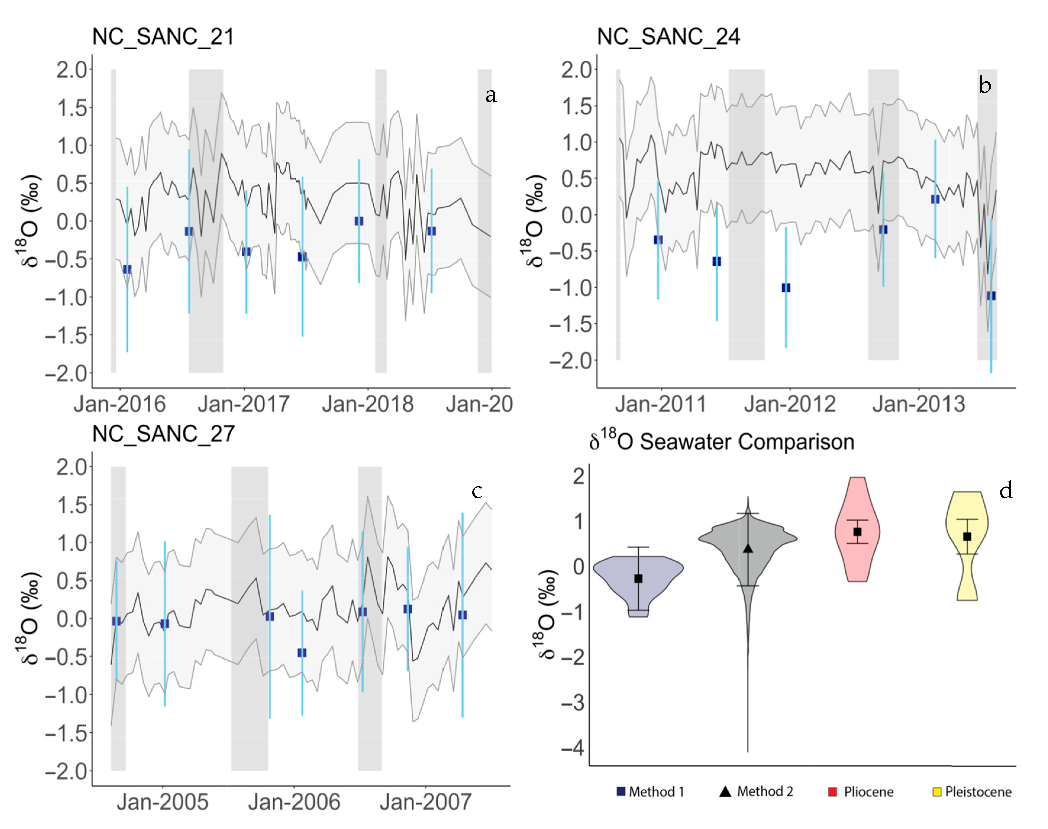
5.3. Comparison of Estimation Methods of Modern δ¹⁸O_sw

Clumped isotope paleothermometry is expected to become a necessary compliment to traditional SST reconstruction studies because reconstructed SST_Δ47 combined with δ¹⁸O_shell values allows estimation of paleo δ¹⁸O_sw. This added value allows evaluation of published δ¹⁸O_sw values based on ice volume models such as the Plio-Pleistocene [32]. We used modern Mercenaria shells to test this approach. Modern δ¹⁸O_sw values were estimated using two methods. Method 1 uses SST_Δ47 and targeted (as defined above) δ¹⁸O_shell values. Method 2 uses measured salinity and the regional δ¹⁸O_sw–salinity relationship (Equation (1)) [72]. As can be seen in Figure 7a–c, the individual SST_Δ47-derived δ¹⁸O_sw values (Method 1) are typically lower than the measured salinity-derived δ¹⁸O_sw values (Method 2) but are within error. Sample NC_SANC_27 shows good agreement between Methods 1 and 2. Like measured salinity, δ¹⁸O_sw values estimated using Methods 1 and 2 do not show seasonal variability; hence, we chose to compare mean δ¹⁸O_sw values between the two methods to see if they produce equivalent results (Hypothesis 3).

Values of δ¹⁸O_sw derived using Method 1 yield a weighted mean of −0.3 ± 0.5‰ (Figure 7d). Values of δ¹⁸O_sw calculated using Method 2 produce a mean of 0.4 ± 0.8‰ (RMSE of the regression). We used a weighted mean for Method 1 because each individual δ¹⁸O_sw value has a propagated SE. The 95% confidence interval for the difference between Methods 1 and 2 ranges from −2‰ to +1‰. Although this interval narrowly includes zero, the distribution is skewed towards negative values, and the central tendency reflects a mean offset of approximately −0.64‰ (Figure 7d). This difference is likely driven by a combination of factors. First, Δ₄₇-derived SST (Method 1) may be biased towards slightly warm temperatures due to analytical uncertainty (warmer than expected during summer; Figure 3) and/or ecological growth bias (i.e., faster growth during optimal SST). Analytical uncertainty in Δ₄₇ measurements, propagated through the Anderson et al. (2021) [79] temperature calibration, contributes a typical SE of ±1.3 to ±2.2 °C. Additional uncertainty arises in the δ¹⁸O_sw calculation due to analytical error in δ¹⁸O_shell values and assumptions about equilibrium fractionation [83]. The result is lower reconstructed δ¹⁸O_sw values. Second, the δ¹⁸O_sw − salinity calibration (Method 2), while regionally appropriate, carries substantial predictive uncertainty (RMSE = 0.8‰) and may not fully capture hydrologic variability during the shell’s growth season. Additionally, the water monitor station in Loosen Creek is located ~1.2 km away from the shell collection site. The shells are closer to shore and could be subjected to localized freshwater input not detected by the water monitor, which would lower the calculated δ¹⁸O_sw values. Taken together, the data suggest that while reconstructed δ¹⁸O_sw values using Methods 1 and 2 are broadly consistent within propagated error, there is a tendency for Method 1 to produce lower values than Method 2. This difference, though not significant, points to important environmental or biological factors influencing the carbonate system that are not fully resolved by salinity-based calibrations alone.

5.4. Paleo SST Reconstructions: Δ₄₇ Versus δ¹⁸O_shell

Most paleoclimate reconstructions using the long-established δ¹⁸O temperature proxy rely on assumed/modeled δ¹⁸O_sw values; however, few studies have validated these values [93,94]. We further tested Hypothesis 2 building on fossil data from our earlier work. Braniecki et al. (2024) [35] reconstructed paleo SST using the δ¹⁸O_shell timeseries from the Duplin and Waccamaw Formations showing differences in average summer and winter temperatures and seasonal amplitudes between the two units. Results from that study also show that they differ from modern conditions. We compared their seasonal results with our summer and winter SSTs_Δ47.

In the Duplin Formation, reconstructed summer SST_Δ47 averages 30 ± 1 °C, while summer SSTs reconstructed from the δ¹⁸O timeseries are 28 ± 1 °C. Winter SST_Δ47 reconstructed from Duplin shells averaged 19 ± 2 °C, compared to winter δ¹⁸O temperature of 18 ± 1 °C. SST_Δ47 shows a seasonal amplitude of ~9 ± 3 °C, while the δ¹⁸O timeseries temperatures are 9 ± 2 °C during the MPWI (Figure 6). The results obtained from these two methods are statistically indistinguishable (summer 95% CI ranges from −2 to +5; winter 95% CI ranges −3 to +7). A Wilcoxon Rank Sum test showed no differences in seasonal amplitude (W = 32, p-value = 0.4742, α = 0.05).

Seasonal data from the Waccamaw shells show different results than data from the Duplin shells. The summer SSTs from the two methods are statistically indistinguishable; however, winter SSTs are not (summer 95% CI ranges from −1 to +7; winter 95% CI ranges +6 to +13). The Wilcoxon Rank Sum test showed statistical differences in the seasonal amplitudes (W = 2, p-value = 0.03501, α = 0.05). Reconstructed summer SST_Δ47 from the Waccamaw shells averaged 25 ± 2 °C compared to δ¹⁸O timeseries summer temperatures of 22 ± 1 °C. Winter SST_Δ47 averaged 20 ± 2 °C, which is significantly higher than the winter SSTs calculated from the δ¹⁸O timeseries (12 ± 1 °C; Figure 6). These high winter SSTs_Δ47 may be due to several factors. First, sample sizes for clumped isotope analysis are much higher than for δ¹⁸O analyses (2 mg vs. 50 μg). This large sample size requires larger drill bit sizes and deeper sampling paths, increasing the amount of time averaging within the shell. This sampling method may incorporate shell material from periods of warmer growth temperatures, thus artificially increasing winter temperatures for Δ₄₇ but not δ¹⁸O estimates. Second, diagenetic alteration over geologic time and interaction with post-depositional fluids have been shown to alter growth temperatures by altering the original isotopic composition of the shells ([95] and references therein). This hypothesis is unlikely, as XRD analysis showed preservation of original aragonite mineralogy and, hence, no evidence of diagenetic alteration [35]. However, solid-state reordering of clumped isotopes has been shown to occur without altering the original isotopic compositions [96] and, thus, would be undetected in XRD analysis. Regardless, temperatures typically need to approach or exceed 100 °C for this to occur [97], which would have been unlikely post-deposition. Friction from the drill bit has been shown to reach temperatures high enough to alter Δ₄₇ values [98], but this is unlikely as we kept our drill speed low (between 1000−3000 rpm), well below the ~15,000 rpm needed for solid-state reordering. Third, the assumed δ¹⁸O_sw values for the early Pleistocene are too low for winter, making the estimated temperature too high. We view this possibility as unlikely and discuss it in more detail in the next section. The most likely explanation for the unexpectedly high SST_Δ47 estimates is within-shell time averaging. Future work should explore different sampling techniques to minimize this time averaging bias.

Similarly to modern δ¹⁸O_sw records, estimated summer and winter Pliocene δ¹⁸O_sw values are statistically indistinguishable from one another (95% CI ranges from −1 to +2). Therefore, we pooled all summer and winter δ¹⁸O_sw values and calculated a weighted mean value. We can compare our weighted mean δ¹⁸O_sw value to widely accepted δ¹⁸O_sw estimates. Our reconstructed δ¹⁸O_sw values for the mid-Pliocene (following Method 1 from Section 5.3) has a weighted mean value of 0.8 ± 0.3‰. Williams et al. (2009) [45] estimated a δ¹⁸O_sw value of 1.1‰ for Virginia during the MPWI based on global circulation models coupled with regional precipitation and evaporation differences, making it more robust than values based on ice volume models. Their value is within the error of our estimate.

Given that (1) our Pliocene data show no statistical seasonal differences and were therefore pooled, and (2) winter SST_Δ47 estimates from the Waccamaw shells are too warm, we only used the summer SSTs_Δ47 from the Waccamaw shells to calculate our reconstructed δ¹⁸O_sw values. Thus, our reconstructed values for the early Pleistocene have a mean of 0.6 ± 0.4‰ (Figure 7d). For comparison, Winkelstern et al. (2013) [20] use a value of 0.0‰ during the early Pleistocene in Virginia, following Krantz (1990) [16]. Their assumed value is lower than our estimate and outside of our error. The combination of SST_Δ47 and δ¹⁸O_shell values shows promise as a method of reconstructing δ¹⁸O_sw values of important time intervals. Given the large errors and small sample size, we are hesitant to establish a new δ¹⁸O_sw value for the early Pleistocene. Future work will add additional samples to more rigorously investigate the δ¹⁸O_sw value for the early Pleistocene.

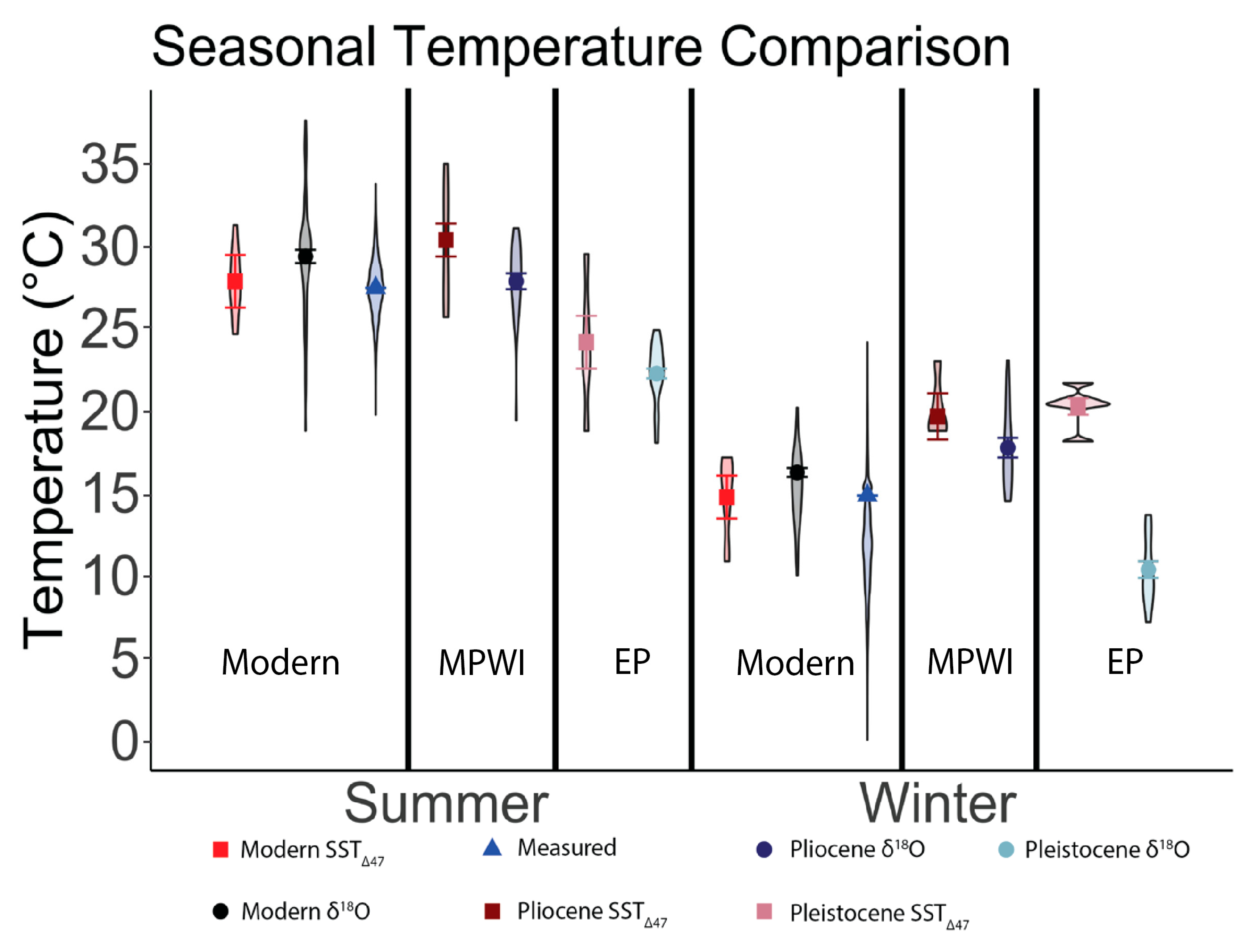
5.5. Comparing Seasonal SST_Δ47 Across Time Intervals

We compared our seasonal SST_Δ47 across the mid-Pliocene, early Pleistocene, and modern time intervals to evaluate any shifts in summer and winter (Hypothesis 4), as well as similarities/differences in seasonal amplitudes (Hypothesis 5). However, because of the potential within-shell time averaging during winter shell growth in the Waccamaw (early-Pleistocene) shells, we focus on the following comparisons: (1) summers across all three time intervals; (2) winters and seasonal amplitudes between the MPWI and modern shells.

Summer SST_Δ47 during the MPWI (30 ± 1 °C) is statistically indistinguishable from modern summer SST_Δ47 (28 ± 2 °C) (95% CI ranges from −6 to +3). For the early Pleistocene, summer SST_Δ47 (25 ± 2 °C) is statistically indistinguishable from modern summer SST_Δ47 (95% CI ranges from −3 to 8). Winter SST_Δ47 values between the MPWI and today are indistinguishable (albeit weakly) from one another (95% CI ranges from −8 to +1). The SST_Δ47 seasonal amplitudes between the MPWI (9 ± 2 °C) and modern shells (14 ± 3 °C) are statistically different (W = 12, p-value = 0.1805, α = 0.05). These differences could be due to a difference in depth. The modern shells and temperature logger were around 1 m in depth, while the Duplin shells come from a ~ 20–30 m depth. However, these depths are within the well-mixed zone and should be subjected to similar temperatures. Similar continental configuration and ocean circulation patterns during the Plio-Pleistocene and today would suggest that it is not unreasonable for similar temperature profiles to exist between the surface and a 30 m depth. Changes in Gulf Stream dynamics have been hypothesized as a mechanism for MPWI warming [3,99]. However, Lee et al. (1991) [100] show that the Gulf Stream is an off-shelf western boundary current and, thus, only reaches as far as the mid-shelf today. Hence, a maximum depth of deposition likely between 20 and 30 m [16] represents inner-shelf conditions and would not be influenced by the Gulf Stream, and the seasonal patterns recorded in our fossil shells are likely not influenced by the Gulf Stream.

We compared our findings with previous studies reporting temperature at seasonal timescales for the MPWI (Krantz, 1990 [16]; Winkelstern et al., 2013 [20]; Johnson et al., 2019 [101]; Johnson et al., 2025 [102]) and early Pleistocene (Krantz, 1990 [15]; Winkelstern et al., 2013 [20]; Johnson et al., 2019 [101]). These studies used fossil shells from the Yorktown Formation of Virginia; Krantz (1990) [16]: Rushmere and Morgarts Beach Members, Chesapecten madisonius and Carolinapecten eboreus; Winkelstern et al. (2013) [20]: Rushmere Member, Mercenaria spp.; Johnson et al. (2019) [101]: Rushmere and Morgarts Beach Members, C. eboreus. Krantz (1990) [16] reports temperatures from two shells representing 1–2 years of growth. We recalculated their temperatures using our calculated δ¹⁸O_sw value of 0.8‰, resulting in a maximum temperature of 35 °C and a minimum of 15 °C. we also recalculated temperatures from Winkelstern et al. (2013) [20] (1920) with our calculated δ¹⁸O_sw value, resulting in a maximum temperature of 31 °C and a minimum temperature of 14 °C based on six shells (4–5 years of growth per shell). Johnson et al. (2019) [101] report on six shells, recording six summers and six winters. Our recalculated temperatures from this study show a maximum summer temperature of 22 °C and minimum temperature of 4 °C. In a later study, Johnson et al. (2025) [102] infer the summer surface temperature based on two of these shells to be 22–29 °C. While Johnson et al. (2025) [102] include Δ₄₇ analysis, they do not explicitly report derived temperature values. The authors do note that there is good agreement between the proxies (see Figure 9 in Johnson et al., 2025 [102]). Summer temperatures for these earlier studies are similar to our summer SST_Δ47. In contrast, the winters from Krantz (1990) [16] and Winkelstern et al. (2013) [20] are 4–5 °C cooler than our winter SST_Δ47, resulting in a larger seasonal amplitude than in our study. The winters from Johnson et al. (2019) [101] are much colder (~14–15 °C) and are likely too cold for the MPWI. One possibility to explain the difference in winter temperatures is the latitude of the respective study localities. The Yorktown Formation in Virginia is ~2–3° N of our collection sites. This small difference in latitude is unlikely to explain a difference of ~5 °C in winter temperature. For a 5 °C difference in winter temperatures, the δ¹⁸O_sw value would need to be ~1‰ lower. Based on the salinity to δ¹⁸O_sw relationship in Elliot et al. (2003) [72], the salinity would be ~5 psu lower than mean seawater. Given these deposits likely represent open-ocean conditions [37], we find this hypothesis unlikely. An alternative explanation is that these formations were not deposited during the same transgression event as previously believed [103,104]. The Yorktown and Duplin Formations have not yet been geochronologically dated and could be part of separate transgression events. Future work aims to date these formations/members and test the hypothesis that they were deposited coevally. We recalculated early-Pleistocene shells with our estimated δ¹⁸O_sw value of 0.6‰. Due to the uncertainty in our SST_Δ47, we only compared summer temperatures. Krantz (1990) [16] reports temperatures from eight shells from the early Pleistocene and reports maximum temperatures of 30 ± 2 °C. Winkelstern et al. (2013) [20] report on six shells from the early Pleistocene which recorded maximum temperatures of 32 °C. Johnson et al. (2019) [101] report on two shells, recording maximum temperatures of 21 °C and 25 °C. These temperatures are more similar to our SST_Δ47. Results from the other previous studies are warmer than our SST_Δ47 by ~5 °C. Using the same δ¹⁸O_sw value, these previous studies are similar to our δ¹⁸O-derived temperatures [35]. Additional samples from the early Pleistocene are needed to further test this hypothesis.

6. Conclusions

Our study compared seasonal growth temperatures derived from δ¹⁸O to those derived from ∆₄₇ in Mercenaria. We show no significant statistical differences between a clumped isotope paleotemperature calibration constructed using Mercenaria and accepted calibrations, indicating that Mercenaria do not require a species-specific calibration. Modern Mercenaria show no distinguishable differences in summer and winter temperatures and seasonal amplitudes between SST_∆47 values and δ¹⁸O_shell temperatures. Different methods to calculate the δ¹⁸O_sw values during the time of shell formation showed no differences in means. Summer and winter temperatures and seasonal amplitudes between SST_∆47 values and δ¹⁸O_shell temperatures during the MPWI were statistically indistinguishable from one another while only summers during the early Pleistocene were indistinguishable from one another. Winter SSTs_∆47 from the early Pleistocene were unusually high and most likely caused by within-shell time averaging. The MPWI had similar summer and winter SST_∆47 values to today but different seasonal amplitudes. This could be due to differences in depth, but this is unlikely due to the depth of the well-mixed zone. Compared to our calculated δ¹⁸O_sw values, modeled values (based on ice volume) are within error for the MPWI but are much lower and not within error for the early Pleistocene. The combination of δ¹⁸O_shell values and ∆₄₇ values is a unique combination that allows for comparisons between derived temperatures and answers questions about δ¹⁸O_sw values in past climate intervals. Additional reconstructions using these proxies will provide an opportunity to unravel past climate conditions to better understand our future.

References

1. Dowsett, H.; Poore, R. Pliocene sea surface temperatures of the North Atlantic Ocean at 3.0 Ma. Quat. Sci. Rev. 1991, 10, 189–204. [Google Scholar] [CrossRef]
2. Thompson, R.S.; Fleming, R.F. Middle Pliocene vegetation: Reconstructions, paleoclimatic inferences, and boundary conditions for climate modeling. Mar. Micropaleontol. 1996, 27, 27–49. [Google Scholar] [CrossRef]
3. Dowsett, H.J.; Chandler, M.A.; Robinson, M.M. Surface temperatures of the Mid-Pliocene North Atlantic Ocean: Implications for future climate. Philos. Trans. Math. Phys. Eng. Sci. 2009, 367, 69–84. [Google Scholar] [CrossRef] [PubMed]
4. Dowsett, H.; Dolan, A.; Rowley, D.; Moucha, R.; Forte, A.M.; Mitrovica, J.X.; Pound, M.; Salzmann, U.; Robinson, M.; Chandler, M.; et al. The PRISM4 (mid-Piacenzian) paleoenvironmental reconstruction. Clim. Past 2016, 12, 1519–1538. [Google Scholar] [CrossRef]
5. Arias, P.; Bellouin, N.; Coppola, E.; Jones, R.; Krinner, G.; Marotzke, J.; Naik, V.; Palmer, M.; Plattner, G.-K.; Rogelj, J. Climate Change 2021: The Physical Science Basis. In Contribution of Working Group I to the Sixth Assessment Report of the Intergovernmental Panel on Climate Change; Technical Summary; Cambridge University Press: Cambridge, UK; New York, NY, USA, 2021. [Google Scholar]
6. Bretherton, F.; Bryan, K.; Woods, J. Time-Dependent Greenhouse-Gas-Induced Climate Change; Cambridge University Press: Cambridge, UK; New York, NY, USA, 1990; pp. 173–194. [Google Scholar]
7. National Weather Service. Annual Average Temperature by Year. U.S. Department of Commerce. Available online: https://www.weather.gov/media/slc/ClimateBook/Annual%20Average%20Temperature%20By%20Year.pdf (accessed on 15 May 2025).
8. Jansen, E.; Overpeck, J.; Briffa, K.R.; Duplessy, J.-C.; Joos, F.; Masson-Delmotte, V.; Olago, D.; Otto-Bliesner, B.; Peltier, W.R.; Rahmstorf, S.; et al. Palaeoclimate. In Contribution of Working Group I to the Fourth Assessment Report of the Intergovernmental Panel on Climate Change; Solomon, S., Qin, D., Manning, M., Chen, Z., Marquis, M., Averyt, K.B., Tignor, M., Miller, H.L., Eds.; Cambridge University Press: Cambridge, UK; New York, NY, USA, 2007. [Google Scholar]
9. Johnson, A.L.A.; Valentine, A.; Leng, M.J.; Sloane, H.J.; Schöne, B.R.; Balson, P.S. Isotopic temperatures from the early and mid-pliocene of the US Middle Atlantic coastal plain, and their implications for the cause of regional marine climate change. Palaios 2017, 32, 250–269. [Google Scholar] [CrossRef]
10. Burke, K.D.; Williams, J.W.; Chandler, M.A.; Haywood, A.M.; Lunt, D.J.; Otto-Bliesne, B.L. Pliocene and Eocene provide best analogs for near-future climates. Proc. Natl. Acad. Sci. USA 2018, 115, 13288–13293. [Google Scholar] [CrossRef]
11. Adopted, I. Climate Change 2014 Synthesis Report; IPCC: Geneva, Switzerland, 2014; pp. 1059–1072. [Google Scholar]
12. Martínez-Botí, M.A.; Foster, G.L.; Chalk, T.B.; Rohling, E.J.; Sexton, P.F.; Lunt, D.J.; Pancost, R.D.; Badger, M.P.S.; Schmidt, D.N. Plio-Pleistocene climate sensitivity evaluated using high-resolution CO2 records. Nature 2015, 518, 49–54. [Google Scholar] [CrossRef]
13. Beierlein, L.; Salvigsen, O.; Schöne, B.R.; Mackensen, A.; Brey, T. The seasonal water temperature cycle in the Arctic Dicksonfjord (Svalbard) during the Holocene Climate Optimum derived from subfossil Arctica islandica shells. Holocene 2015, 25, 1197–1207. [Google Scholar] [CrossRef]
14. Mouchi, V.; Godbillot, C.; Forest, V.; Ulianov, A.; Lartaud, F.; de Rafélis, M.; Emmanuel, L.; Verrecchia, E.P. Rare earth elements in oyster shells: Provenance discrimination and potential vital effects. Biogeosciences 2020, 17, 2205–2217. [Google Scholar] [CrossRef]
15. Quitmyer, I.R.; Hale, H.S.; Jones, D.S. Paleoseasonality Determination Based on Incremental Shell Growth in the Hard Clam, Mercenaria mercenaria, and its Implications for the Analysis of Three Southeast Georgia Coastal Shell Middens. Southeast. Archaeol. 1985, 4, 27–40. [Google Scholar]
16. Krantz, D.E. Mollusk-isotope records of Plio-Pleistocene marine paleoclimate, U.S. Middle Atlantic Coastal Plain. Palaios 1990, 5, 317–335. [Google Scholar] [CrossRef]
17. Ward, L.W.; Bailey, R.; Carter, J.; Horton, J.; Zullo, V.A. Pliocene and early Pleistocene stratigraphy, depositional history, and molluscan paleobiogeography of the Coastal Plain. In The Geology Of The Carolinas; University of Tennessee Press: Knoxville, TN, USA, 1991; pp. 274–289. [Google Scholar]
18. Jones, D.S.; Allmon, W.D. Records of upwelling, seasonality and growth in stable-isotope profiles of Pliocene mollusk shells from Florida. Lethaia 1995, 28, 61–74. [Google Scholar] [CrossRef]
19. Jones, D.S.; Quitmyer, I.R. Marking Time with Bivalve Shells: Oxygen Isotopes and Season of Annual Increment Formation. Palaios 1996, 11, 340–346. [Google Scholar] [CrossRef]
20. Winkelstern, I.; Surge, D.; Hudley, J.W. Multiproxy Sclerochronological Evidence for Plio-Pleistocene Regional Warmth: United State Mid-Atlantic Coastal Plain. Palaios 2013, 28, 649–660. [Google Scholar] [CrossRef]
21. Goodwin, D.H.; Scho, B.R.; Dettman, D.L. Resolution and Fidelity of Oxygen Isotopes as Paleotemperature Proxies in Bivalve Mollusk Shells: Models and Observations. Palaios 2003, 18, 110–125. [Google Scholar] [CrossRef]
22. Gillikin, D.P.; De Ridder, F.; Ulens, H.; Elskens, M.; Keppens, E.; Baeyens, W.; Dehairs, F. Assessing the reproducibility and reliability of estuarine bivalve shells (Saxidomus giganteus) for sea surface temperature reconstruction: Implications for paleoclimate studies. Palaeogeogr. Palaeoclimatol. Palaeoecol. 2005, 228, 70–85. [Google Scholar] [CrossRef]
23. Quitmyer, I.R.; Jones, D.S.; Arnold, W.S. The Sclerochronology of Hard Clams, Mercenaria spp., from the South-Eastern U.S.A.: A Method of Elucidating the Zooarchaeological Records of Seasonal Resource Procurement and Seasonality in Prehistoric Shell Middens. J. Archaeol. Sci. Rep. 1997, 24, 825–840. [Google Scholar] [CrossRef]
24. Ansell, A.D. The Rate of Growth of the Hard Clam (Mercenaria mercenaria) throughout the Geographical Range. ICES J. Mar. Sci. 1968, 31, 364–409. [Google Scholar] [CrossRef]
25. Wang, T.; Surge, D.; Walker, K.J. Isotopic evidence for climate change during the Vandal Minimum from Ariopsis felis otoliths and Mercenaria campechiensis shells, southwest Florida, USA. Holocene 2011, 21, 1081–1091. [Google Scholar] [CrossRef]
26. Stenzel, H.B. Ancestors of the quahog. J. Sediment. Res. 1955, 25, 145. [Google Scholar] [CrossRef]
27. Harte, M.E. Chapter 1 Systematics and taxonomy. In Developments in Aquaculture and Fisheries Science; Kraeuter, J.N., Castagna, M., Eds.; Elsevier: Amsterdam, The Netherlands, 2001; pp. 3–51. [Google Scholar]
28. Zachos, J.; Pagani, M.; Sloan, L.; Thomas, E.; Billups, K. Trends, Rhythms, and Aberrations in Global Climate 65 Ma to Present. Science 2001, 292, 686–693. [Google Scholar] [CrossRef]
29. Lutringer, A.; Blamart, D.; Frank, N.; Labeyrie, L. Paleotemperatures from deep-sea corals: Scale effects. In Cold-Water Corals and Ecosystems; Freiwald, A., Roberts, J.M., Eds.; Springer: Berlin/Heidelberg, Germany, 2005; pp. 1081–1096. [Google Scholar]
30. Ghosh, P.; Adkins, J.; Affek, H.; Balta, B.; Guo, W.; Schauble, E.A.; Schrag, D.; Eiler, J.M. 13C–18O bonds in carbonate minerals: A new kind of paleothermometer. Geochim. Cosmochim. Acta 2006, 70, 1439–1456. [Google Scholar] [CrossRef]
31. Schauble, E.A.; Ghosh, P.; Eiler, J.M. Preferential formation of 13C–18O bonds in carbonate minerals, estimated using first-principles lattice dynamics. Geochim. Cosmochim. Acta 2006, 70, 2510–2529. [Google Scholar] [CrossRef]
32. Huntington, K.W.; Budd, D.A.; Wernicke, B.P.; Eiler, J.M. Use of Clumped-Isotope Thermometry To Constrain the Crystallization Temperature of Diagenetic Calcite. J. Sediment. Res. 2011, 81, 656–669. [Google Scholar] [CrossRef]
33. Briggs, J.C.; Bowen, B.W. A realignment of marine biogeographic provinces with particular reference to fish distributions. J. Biogeogr. 2012, 39, 12–30. [Google Scholar] [CrossRef]
34. Rovere, A.; Hearty, P.J.; Austermann, J.; Mitrovica, J.X.; Gale, J.; Moucha, R.; Forte, A.M.; Raymo, M.E. Mid-Pliocene shorelines of the US Atlantic Coastal Plain—An improved elevation database with comparison to Earth model predictions. Earth-Sci. Rev. 2015, 145, 117–131. [Google Scholar] [CrossRef]
35. Braniecki, G.F.; Surge, D.; Hyland, E.G.; Goodwin, D.H. Reconstructed seasonality during the Mid Piacenzian Warm Interval and early Pleistocene cooling as recorded by growth temperatures from Mercenaria shells. Quat. Sci. Rev. 2024, 328, 108524. [Google Scholar] [CrossRef]
36. Ward, L.W.; Blackwelder, B.W. Stratigraphic Revision of Upper Miocene and Lower Pliocene Beds of the Chesapeake Group, Middle Atlantic Coastal Plain; Bulletin; U.S. Geological Survey: Reston, VA, USA, 1980. [Google Scholar]
37. Blackwelder, B.W. Late Cenozoic Stages and Molluscan Zones of the U.S. Middle Atlantic Coastal Plain. J. Paleontol. 1981, 55 (Suppl. S12), 1–34. [Google Scholar] [CrossRef]
38. Krantz, D.E. A chronology of Pliocene sea-level fluctuations: The U.S. Middle Atlantic Coastal Plain record. Quat. Sci. Rev. 1991, 10, 163–174. [Google Scholar] [CrossRef]
39. Ward, L.W.; Gilinsky, N.L. Molluscan Assemblages of the Chowan River Formation; Virginia Museum of Natural History: Martinsville, VA, USA, 1993. [Google Scholar]
40. Groot, J.J. Palynological evidence for late Miocene, Pliocene and early Pleistocene climate changes in the middle US Atlantic coastal plain. Quat. Sci. Rev. 1991, 10, 147–162. [Google Scholar] [CrossRef]
41. Snyder, S.W.; Mauger, L.L.; Ames, D. Benthic Foraminifera and Paleecology of the Pliocene Yorktown and Chowan River Formations, Lee Creek Mine, North Carolina, USA. J. Foraminifer. Res. 2001, 31, 244–274. [Google Scholar] [CrossRef]
42. Ward, L.W. Geology and Paleontology of the James River: Richmond to Hampton Roads; Virginia Museum of Natural History: Martinsville, VA, USA, 2008. [Google Scholar]
43. Cronin, T.W. Evolution of marine climates of the US Atlantic coast during the past four million years. Philos. Trans. R. Soc. B Biol. Sci. 1988, 318, 661–678. [Google Scholar]
44. Dowsett, H.J.; Cronin, T.M. High eustatic sea level during the middle Pliocene: Evidence from the southeastern US Atlantic Coastal Plain. Geology 1990, 18, 435–438. [Google Scholar] [CrossRef]
45. Williams, M.; Haywood, A.M.; Harper, E.M.; Johnson, A.L.A.; Knowles, T.; Leng, M.J.; Lunt, D.J.; Okamura, B.; Taylor, P.D.; Zalasiewicz, J. Pliocene climate and seasonality in North Atlantic shelf seas. Philos. Trans. R. Soc. A 2009, 367, 85–108. [Google Scholar] [CrossRef] [PubMed]
46. Dowsett, H.; Robinson, M.; Haywood, A.M.; Salzmann, U.; Hill, D.; Sohl, L.E.; Chandler, M.; Williams, M.; Foley, K.; Stoll, D.K. The PRISM3D paleoenvironmental reconstruction. Stratigraphy 2010, 7, 123–139. [Google Scholar] [CrossRef]
47. Haywood, A.M.; Hill, D.J.; Dolan, A.M.; Otto-Bliesner, B.L.; Bragg, F.; Chan, W.L.; Chandler, M.A.; Contoux, C.; Dowsett, H.J.; Jost, A.; et al. Large-scale features of Pliocene climate: Results from the Pliocene Model Intercomparison Project. Clim. Past 2013, 9, 191–209. [Google Scholar] [CrossRef]
48. Dowsett, H.J.; Wiggs, L.B. Planktonic foraminiferal assemblage of the Yorktown Formation, Virginia, USA. Micropaleontology 1992, 38, 75–86. [Google Scholar] [CrossRef]
49. Dowsett, H.J.; Robinson, M.M.; Foley, K.M.; Herber, T.D. The Yorktown Formation: Improved stratigraphy, chronology, and paleoclimate interpretations from the US mid-Atlantic Coastal Plain. Geosciences 2021, 11, 486. [Google Scholar] [CrossRef]
50. Lisiecki, L.E.; Raymo, M.E. A Pliocene-Pleistocene stack of 57 globally distributed benthic δ18O records. Paleoceanography 2005, 20, PA1003. [Google Scholar]
51. Hazel, J.E. Distribution of some biostratigraphically diagnostic ostracodes in the Pliocene and lower Pleistocene of Virginia and northern North Carolina. Bull. U.S. Geol. J. Res. 1977, 5, 373–388. [Google Scholar]
52. Gibbard, P.L.; Head, M.J.; Walker, M.J.C.; Subcommission on Quaternary Stratigraph. Formal ratification of the Quaternary System/Period and the Pleistocene Series/Epoch with a base at 2.58 Ma. J. Quat. Sci. 2010, 25, 96–102. [Google Scholar] [CrossRef]
53. Merrill, A.S.; Ropes, J. Distribution of southern quahogs off the middle Atlantic coast. Commer. Fish. Rev. 1967, 29, 62–64. [Google Scholar]
54. Arnold, W.; Bert, T.; Quitmyer, I.; Jones, D. Contemporaneous deposition of annual growth bands in Mercenaria mercenaria (Linnaeus), Mercenaria campechiensis (Gmelin), and their natural hybrid forms. J. Exp. Mar. Biol. Ecol. 1998, 223, 93–109. [Google Scholar] [CrossRef]
55. MacKenzie, C.L., Jr.; Morrison, A.; Taylor, D.L.; Burrell, V.G., Jr.; Arnold, W.S.; Wakida-Kusunoki, A.T. Quahogs in eastern North America: Part I, biology, ecology, and historical uses. Mar. Fish. Rev. 2002, 64, 1–56. [Google Scholar]
56. National Marine Fisheries Service. Fisheries of the United States, 2019; U.S. Department of Commerce, NOAA Current Fishery Statistics No. 2019; 2021. Available online: https://media.fisheries.noaa.gov/2021-05/FUS2019-FINAL-webready-2.3.pdf (accessed on 1 April 2021).
57. Kraeuter, J.N.; Castagna, M. Biology of the Hard Clam; Elsevier: Amsterdam, The Netherlands, 2001. [Google Scholar]
58. Grizzle, R.E.; Bricelj, V.M.; Shumway, S.E. Chapter 8 Physiological ecology of Mercenaria mercenaria. In Developments in Aquaculture and Fisheries Science; Kraeuter, J.N., Castagna, M., Eds.; Elsevier: Amsterdam, The Netherlands, 2001; pp. 305–382. [Google Scholar]
59. Jones, D.S.; Arthur, M.A.; Allard, D.J. Sclerochronological records of temperature and growth from shells of Mercenaria mercenaria from Narragansett Bay, Rhode Island. Mar. Biol. 1989, 102, 225–234. [Google Scholar] [CrossRef]
60. Briggs, J.C. Global Biogeography; Elsevier: Amsterdam, The Netherlands, 1995. [Google Scholar]
61. Sato, S.i. Spawning periodicity and shell microgrowth patterns of the venerid bivalve Phacosoma japonicum (Reeve, 1850). Veliger 1995, 38, 61–72. [Google Scholar]
62. Kennedy, H.; Richardson, C.; Duarte, C.; Kennedy, D. Oxygen and carbon stable isotopic profiles of the fan mussel, Pinna nobilis, and reconstruction of sea surface temperatures in the Mediterranean. Mar. Biol. 2001, 139, 1115–1124. [Google Scholar] [CrossRef]
63. Fritz, L.W. Shell Structure and Age Determination, in Developments in Aquaculture and Fisheries Science; Elsevier: Amsterdam, The Netherlands, 2001; pp. 53–76. [Google Scholar]
64. Pannella, G.; MacClintock, C. Biological and Environmental Rhythms Reflected in Molluscan Shell Growth. Mem. (Paleontol. Soc.) 1968, 2, 64–80. [Google Scholar] [CrossRef]
65. Rhoads, D.C.; Pannella, G. The use of molluscan shell growth patterns in ecology and paleoecology. Lethaia 1970, 3, 143–161. [Google Scholar] [CrossRef]
66. Clark, G.R. Seasonal growth variations in the shells of recent and prehistoric specimens of Mercenaria mercenaria from St. Catherines Island, Georgia. Anthropol. Pap. Am. Mus. Nat. Hist. 1979, 51, 161–179. [Google Scholar]
67. Fritz, L.W. Annulus Formation and Microstructure of Hard Clam (Mercenaria mercenaria) Shells. Master’s Thesis, School of Marine Science, College of William and Mary, Virginia Institute of Marine Science, Gloucester Point, VA, USA, 1982. [Google Scholar]
68. Jones, D.S.; Quitmyer, I.R.; Arnold, W.S.; Marelli, D. Annual shell banding, age, and growth rate of hard clams (Mercenaria spp.) from Florida. J. Shellfish Res. 1990, 9. [Google Scholar]
69. Arnold, W.S.; Marelli, D.C.; Bert, T.M.; Jones, D.S.; Quitmyer, I.R. Habitat-specific growth of hard clams Mercenaria mercenaria (L.) from the Indian River, Florida. J. Exp. Mar. Biol. Ecol. 1991, 147, 245–265. [Google Scholar] [CrossRef]
70. Surge, D.; Wang, T.; Gutièrrez-Zugasti, I.; Kelley, P.H. Isotope Sclerochronology and Season of Annual Growt Line Formation in Limpet Shells (Patella Vulgata) from Warm- and Cold- Temperate Zones in the Eastern North Atlantic. Palaios 2013, 28, 386–393. [Google Scholar] [CrossRef]
71. Henry, K.M.; Cerrato, R.M. The Annual Macroscopic Growth Pattern Of The Northern Quahog [=Hard Clam, Mercenaria mercenaria (L.)], In Narragansett Bay, Rhode Island. J. Shellfish Res. 2007, 26, 985–993, 9. [Google Scholar] [CrossRef]
72. Elliot, M.; de Menocal, P.B.; Linsley, B.K.; Howe, S.S. Environmental controls on the stable isotopic composition of Mercenaria mercenaria: Potential application to paleoenvironmental studies. Geochem. Geophys. Geosyst. 2003, 4, 7. [Google Scholar] [CrossRef]
73. Kubota, K.; Shirai, K.; Murakami-Sugihara, N.; Seike, K.; Hori, M.; Tanabe, K. Annual shell growth pattern of the Stimpson’s hard clam Mercenaria stimpsoni as revealed by sclerochronological and oxygen stable isotope measurements. Palaeogeogr. Palaeoclimatol. Palaeoecol. 2017, 465, 307–315. [Google Scholar] [CrossRef]
74. Palmer, K.L.; Moss, D.K.; Surge, D.; Turek, S. Life history patterns of modern and fossil Mercenaria spp. from warm vs. cold climates. Palaeogeogr. Palaeoclimatol. Palaeoecol. 2021, 566, 110227. [Google Scholar] [CrossRef]
75. Kidwell, S. Time-averaging in the marine fossil record: Overview of strategies and uncertainties. Oceanogr. Lit. Rev. 1998, 9, 1546–1547. [Google Scholar] [CrossRef]
76. Bernasconi, S.M.; Daëron, M.; Bergmann, K.D.; Bonifacie, M.; Meckler, A.N.; Affek, H.P.; Anderson, N.; Bajnai, D.; Barkan, E.; Beverly, E.; et al. InterCarb: A Community Effort to Improve Interlaboratory Standardization of the Carbonate Clumped Isotope Thermometer Using Carbonate Standards. Geochem. Geophys. Geosyst. 2021, 22, e2020GC009588. [Google Scholar] [CrossRef]
77. John, C.M.; Bowen, D. Community software for challenging isotope analysis: First applications of ‘Easotope’ to clumped isotopes. Rapid Commun. Mass Spectrom. 2016, 30, 2285–2300. [Google Scholar] [CrossRef]
78. Daëron, M. Full Propagation of Analytical Uncertainties in Δ47 Measurements. Geochem. Geophys. Geosystems 2021, 22, e2020GC009592. [Google Scholar] [CrossRef]
79. Anderson, N.T.; Kelson, J.R.; Kele, S.; Daëron, M.; Bonifacie, M.; Horita, J.; Mackey, T.J.; John, C.M.; Kluge, T.; Petschnig, P.; et al. A Unified Clumped Isotope Thermometer Calibration (0.5–1,100°C) Using Carbonate-Based Standardization. Geophys. Res. Lett. 2021, 48, e2020GL092069. [Google Scholar] [CrossRef]
80. Brand, W.A.; Assonov, S.S.; Coplen, T.B. Correction for the 17O interference in δ(13C) measurements when analyzing CO2 with stable isotope mass spectrometry. Pure Appl. Chem. 2010, 82, 1719–1733. [Google Scholar] [CrossRef]
81. Urey, H.C. Oxygen Isotopes in Nature and in the Laboratory. Science 1948, 108, 489–496. [Google Scholar] [CrossRef]
82. Epstein, S.; Buchsbaum, R.; Lowenstam, H.A.; Urey, H.C. Revised Carbonate-Water Isotopic Temperature Scale. GSA Bull. 1953, 64, 1315–1326. [Google Scholar] [CrossRef]
83. Grossman, E.L.; Ku, T.-L. Oxygen and carbon isotope fractionation in biogenic aragonite: Temperature effects. Chem. Geol. Isot. Geosci. Sect. 1986, 59, 59–74. [Google Scholar] [CrossRef]
84. Dettman, D.L.; Reische, A.K.; Lohmann, K.C. Controls on the stable isotope composition of seasonal growth bands in aragonitic fresh-water bivalves (unionidae). Geochim. Cosmochim. Acta 1999, 63, 1049–1057. [Google Scholar] [CrossRef]
85. Gonfiantini, R.; Stichler, W.; Rozanski, K. Standards and Intercomparison Materials Distributed by the International Atomic Energy Agency for Stable Isotope Measurements; IAEA: Vienna, Austria, 1995. [Google Scholar]
86. Beck, J.W.; Edwards, R.L.; Ito, E.; Taylor, F.W.; Recy, J.; Rougerie, F.; Joannot, P.; Henin, C. Sea-surface temperature from coral skeletal strontium/calcium ratios. Science 1992, 257, 644–647. [Google Scholar] [CrossRef]
87. Klein, R.T.; Lohmann, K.C.; Thayer, C.W. Bivalve skeletons record sea-surface temperature and δ18O via Mg/Ca and 18O/16O ratios. Geology 1996, 24, 415–418. [Google Scholar] [CrossRef]
88. Surge, D.; Lohmann, K.C.; Dettman, D.L. Controls on isotopic chemistry of the American oyster, Crassostrea virginica: Implications for growth patterns. Palaeogeogr. Palaeoclimatol. Palaeoecol. 2001, 172, 283–296. [Google Scholar] [CrossRef]
89. Petersen, S.V.; Defliese, W.F.; Saenger, C.; Daëron, M.; Huntington, K.W.; John, C.M.; Kelson, J.R.; Bernasconi, S.M.; Colman, A.S.; Kluge, T.; et al. Effects of Improved 17O Correction on Interlaboratory Agreement in Clumped Isotope Calibrations, Estimates of Mineral-Specific Offsets, and Temperature Dependence of Acid Digestion Fractionation. Geochem. Geophys. Geosyst. 2019, 20, 3495–3519. [Google Scholar] [CrossRef]
90. Jautzy, J.J.; Savard, M.M.; Dhillon, R.S.; Bernasconi, S.M.; Smirnoff, A. Clumped isotope temperature calibration for calcite: Bridging theory and experimentation. Geochem. Perspect. Lett. 2020, 14, 36–41. [Google Scholar] [CrossRef]
91. Huyghe, D.; Daëron, M.; de Rafelis, M.; Blamart, D.; Sébilo, M.; Paulet, Y.-M.; Lartaud, F. Clumped isotopes in modern marine bivalves. Geochim. Cosmochim. Acta 2022, 316, 41–58. [Google Scholar] [CrossRef]
92. Eagle, R.A.; Eiler, J.M.; Tripati, A.K.; Ries, J.B.; Freitas, P.S.; Hiebenthal, C.; Wanamaker, A.D., Jr.; Taviani, M.; Elliot, M.; Marenssi, S.; et al. The influence of temperature and seawater carbonate saturation state on 13C–18O bond ordering in bivalve mollusks. Biogeosciences 2013, 10, 4591–4606. [Google Scholar] [CrossRef]
93. Cummins, R.C.; Finnegan, S.; Fike, D.A.; Eiler, J.M.; Fischer, W.W. Carbonate clumped isotope constraints on Silurian ocean temperature and seawater δ18O. Geochim. Cosmochim. Acta 2014, 140, 241–258. [Google Scholar] [CrossRef]
94. Henkes, G.A.; Passey, B.H.; Grossman, E.L.; Shenton, B.J.; Yancey, T.E.; Pérez-Huerta, A. Temperature evolution and the oxygen isotope composition of Phanerozoic oceans from carbonate clumped isotope thermometry. Earth Planet. Sci. Lett. 2018, 490, 40–50. [Google Scholar] [CrossRef]
95. Swart, P.K. The geochemistry of carbonate diagenesis: The past, present and future. Sedimentology 2015, 62, 1233–1304. [Google Scholar] [CrossRef]
96. Henkes, G.A.; Passey, B.H.; Grossman, E.L.; Shenton, B.J.; Pérez-Huerta, A.; Yancey, T.E. Temperature limits for preservation of primary calcite clumped isotope paleotemperatures. Geochim. Cosmochim. Acta 2014, 139, 362–382. [Google Scholar] [CrossRef]
97. Winkelstern, I.Z.; Lohmann, K.C. Shallow burial alteration of dolomite and limestone clumped isotope geochemistry. Geology 2016, 44, 467–470. [Google Scholar] [CrossRef]
98. Staudigel, P.T.; Swart, P.K. Isotopic behavior during the aragonite-calcite transition: Implications for sample preparation and proxy interpretation. Chem. Geol. 2016, 442, 130–138. [Google Scholar] [CrossRef]
99. Auderset, A.; Martínez-García, A.; Tiedemann, R.; Hasenfratz, A.P.; Eglinton, T.I.; Schiebel, R.; Sigman, D.M.; Haug, G.H. Gulf Stream intensification after the early Pliocene shoaling of the Central American Seaway. Earth Planet. Sci. Lett. 2019, 520, 268–278. [Google Scholar] [CrossRef]
100. Lee, T.N.; Yoder, J.A.; Atkinson, L.P. Gulf Stream frontal eddy influence on productivity of the southeast U.S. continental shelf. J. Geophys. Res. Ocean. 1991, 96, 22191–22205. [Google Scholar] [CrossRef]
101. Johnson, A.L.A.; Valentine, A.M.; Leng, M.J.; Schöne, B.R.; Sloane, H.J. Life History, Environment and Extinction of the Scallopcarolinapecten Eboreus(Conrad) in the Plio-Pleistocene of the U.S. Eastern Seaboard. Palaios 2019, 34, 49–70. [Google Scholar] [CrossRef]
102. Johnson, A.L.A.; Schöne, B.R.; Petersen, S.V.; de Winter, N.J.; Dowsett, H.J.; Cudennec, J.-F.; Harper, E.M.; Winkelstern, I.Z. Molluscan isotope sclerochronology in marine palaeoclimatology: Taxa, technique and timespan issues. Quat. Sci. Rev. 2025, 350, 109068. [Google Scholar] [CrossRef]
103. Hazel, J.E. Ostracode Biostratigraphy of the Yorktown Formation: (Upper Miocene and Lower Pliocene) of Virginia and North Carolina; US Government Printing Office: Washington, DC, USA, 1971; Volume 704.
104. Hazel, J.E. Age and correlation of the Yorktown (Pliocene) and Croatan (Pliocene and Pleistocene) formations at the Lee Creek Mine. Smithson. Contrib. Paleobiol. 1983, 53, 81–199. [Google Scholar]
Figure 1. Cross-section photomicrograph of M. mercenaria specimen NC_SANC_27. Light increments (white) represent periods of fast growth. Dark increments (purple) represent periods of slowed growth. Growth direction from left to right. Bar = 1 cm.
Geosciences 15 00295 g001
Figure 2. (a) Map showing sampling locations for live-collected and fossil shells and Plio-Pleistocene shorelines of MACP. Paleoshoreline modeled after Rovere et al. (2015) [34]. (b) Site map showing site of live-collected specimens (yellow dot) and location of National Estuarine Research Reserve System water monitor (green dot). Modified from Braniecki et al. (2024) [35].
Geosciences 15 00295 g002
Figure 3. δ18Oshell (black line) records from live-collected M. mercenaria shells. X-axis represents time in years, with each tick mark representing 1 January. Gray line represents measured temperature from nearby (~2 km away) water monitoring station. Gray boxes represent dark increments within shells. Temperature on left Y-axis, calculated using equilibrium equation for aragonite from Dettman et al., (1999) [82]. Red squares represent ∆47-derived temperatures and orange triangles represent δ18O-derived temperatures from δ18O values collected during clumped isotope analysis. Error bars represent one SE. We used paleotemperature calibration published by Anderson et al. (2021) [79] to derive temperatures from ∆47 values.
Geosciences 15 00295 g003
Figure 4. δ18Oshell (black line) records from Plio-Pleistocene M. mercenaria shells. X-axis represents distance from umbo in mm. Gray boxes represent dark increments within shells. Temperature on left Y-axis, calculated using equilibrium equation for aragonite from Dettman et al., (1999) [83]. Red squares represent ∆47-derived temperatures and orange triangles represent δ18O-derived temperatures from δ18O values collected during clumped isotope analysis. Error bars represent one SE. We used paleotemperature calibration published by Anderson et al. (2021) [79] to derive temperatures from ∆47 values. Boxes arranged in stratigraphic order, with Pliocene shells on bottom and Pleistocene shells on top.
Geosciences 15 00295 g004
Figure 5. Comparison of our ∆47 paleotemperature calibration (black) to previously published calibrations. Black circles = individual samples. Colors correspond to the color of the referenced study. Black = this study; Red = Eagle et al. (2013) [92]; Blue = Petersen et al. (2019) [89]; Green = Jautzy et al. (2020) [90]; Orange = Anderson et al. (2021) [79]; Purple = Huyghe et al. (2021) [91]. Dotted lines use ARF reference frame. Dashed lines update reference frame to include 17O corrections and acid fractionation factors. Solid lines use I-CDES reference frame.
Geosciences 15 00295 g005
Figure 6. Violin plots of temperature from modern, MPWI, and early Pleistocene (EP) shells and recorded temperatures from North Carolina. Violins show distribution of each group. Means and SEs of means represented by corresponding shape and error bars.
Geosciences 15 00295 g006
Figure 7. (ac) δ18Osw (black line) records from Method 2 (see text). Gray ribbon represents one SE. X-axis represents time in years, with each tick mark representing 1 January. Gray boxes represent dark increments within shells. Blue squares represent δ18Osw estimated Method 1 (see text). Error bars represent one SE. (d) Comparison of average δ18Osw values from modern shells (blue), measured (black), Pliocene (red), and Pleistocene (yellow). Violins show distribution of each group. Means and SEs of means represented by corresponding shape and error bars.
Geosciences 15 00295 g007