
Experimental Seismic Surveying in a Historic Underground Metals Mine


Abstract
1. Introduction
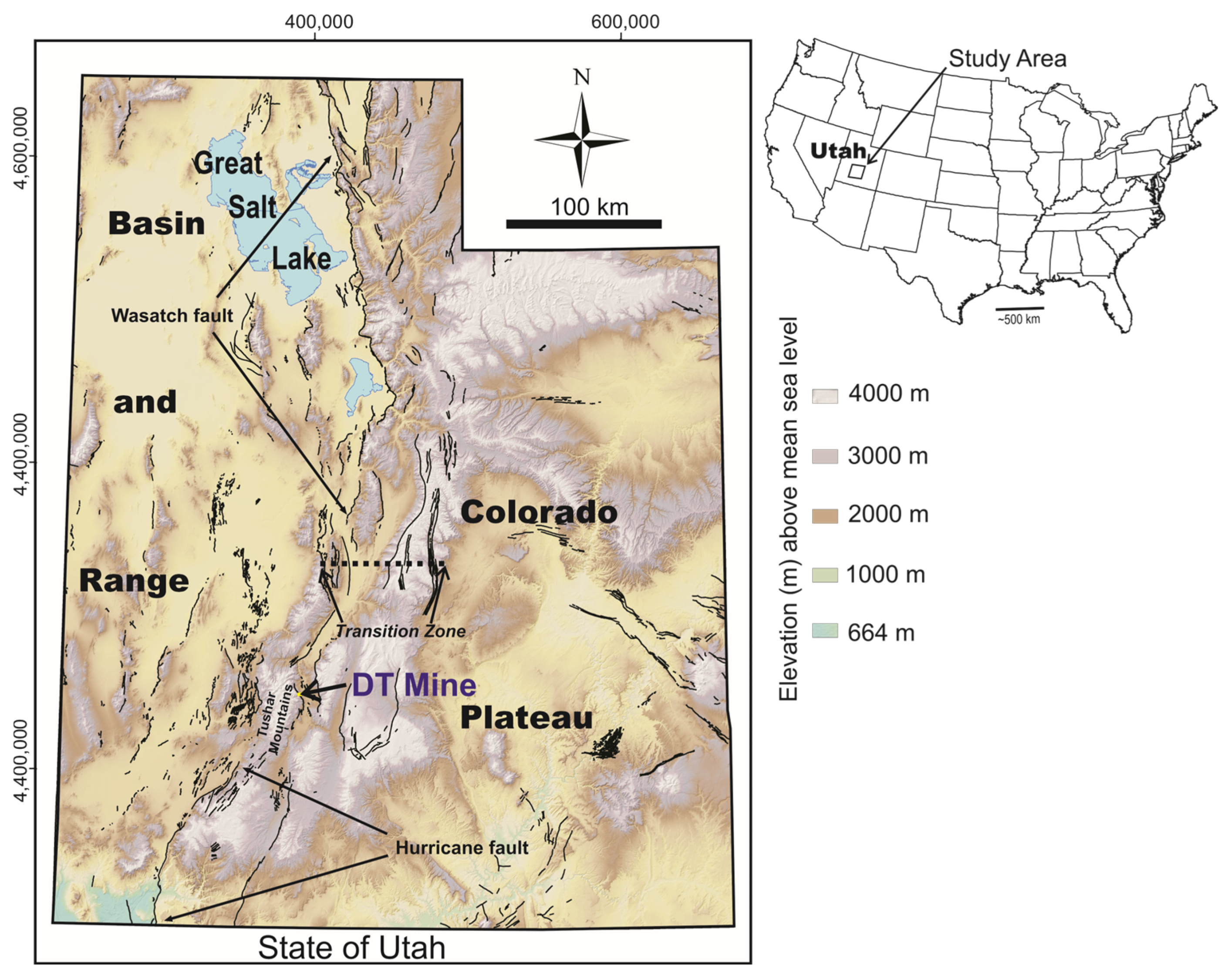
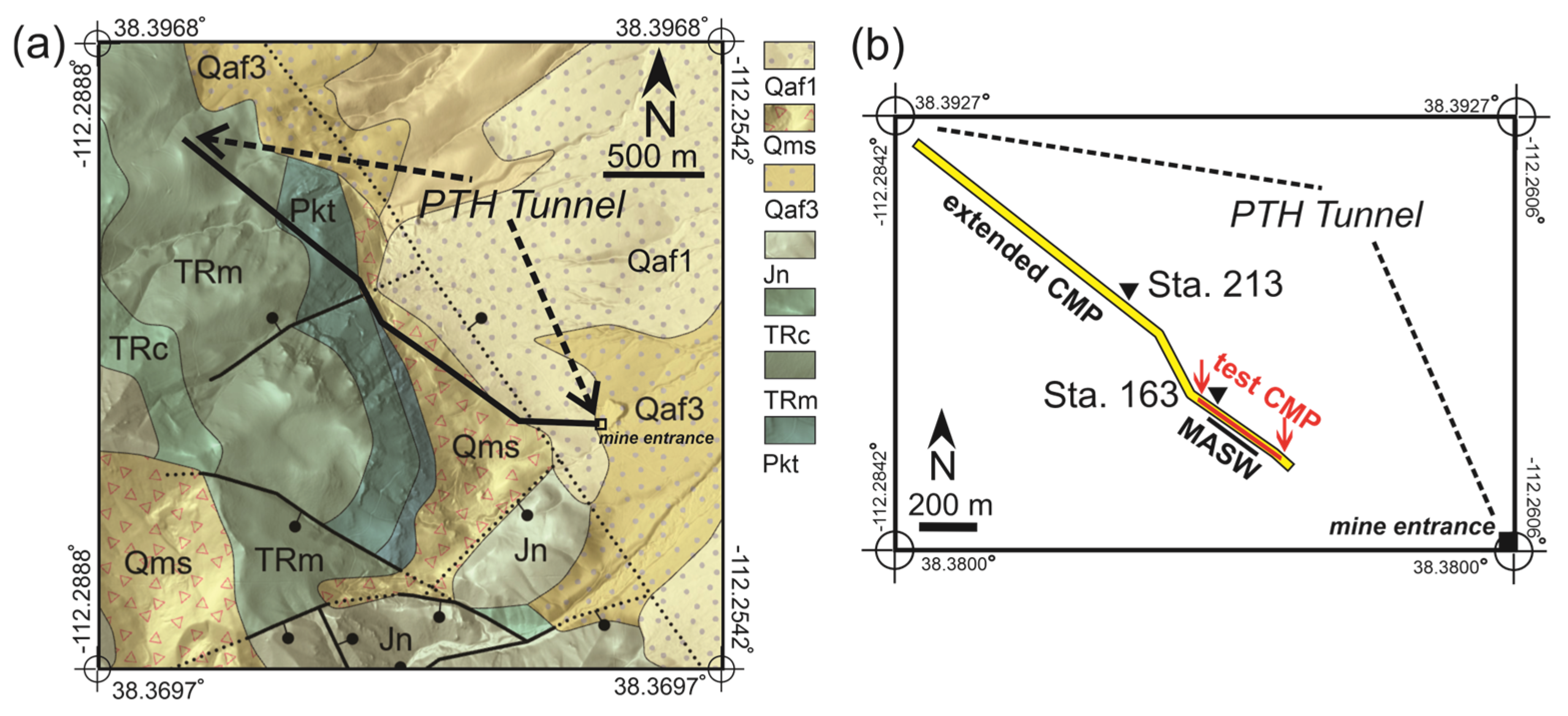
2. Geologic Setting
3. Methods
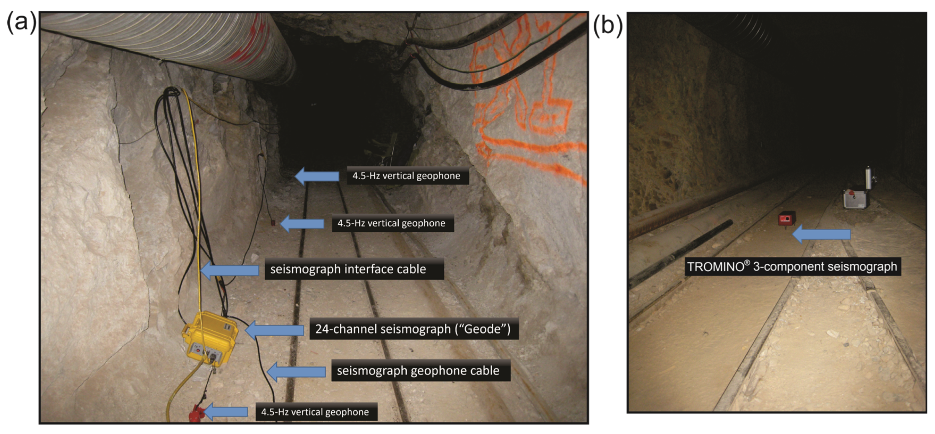
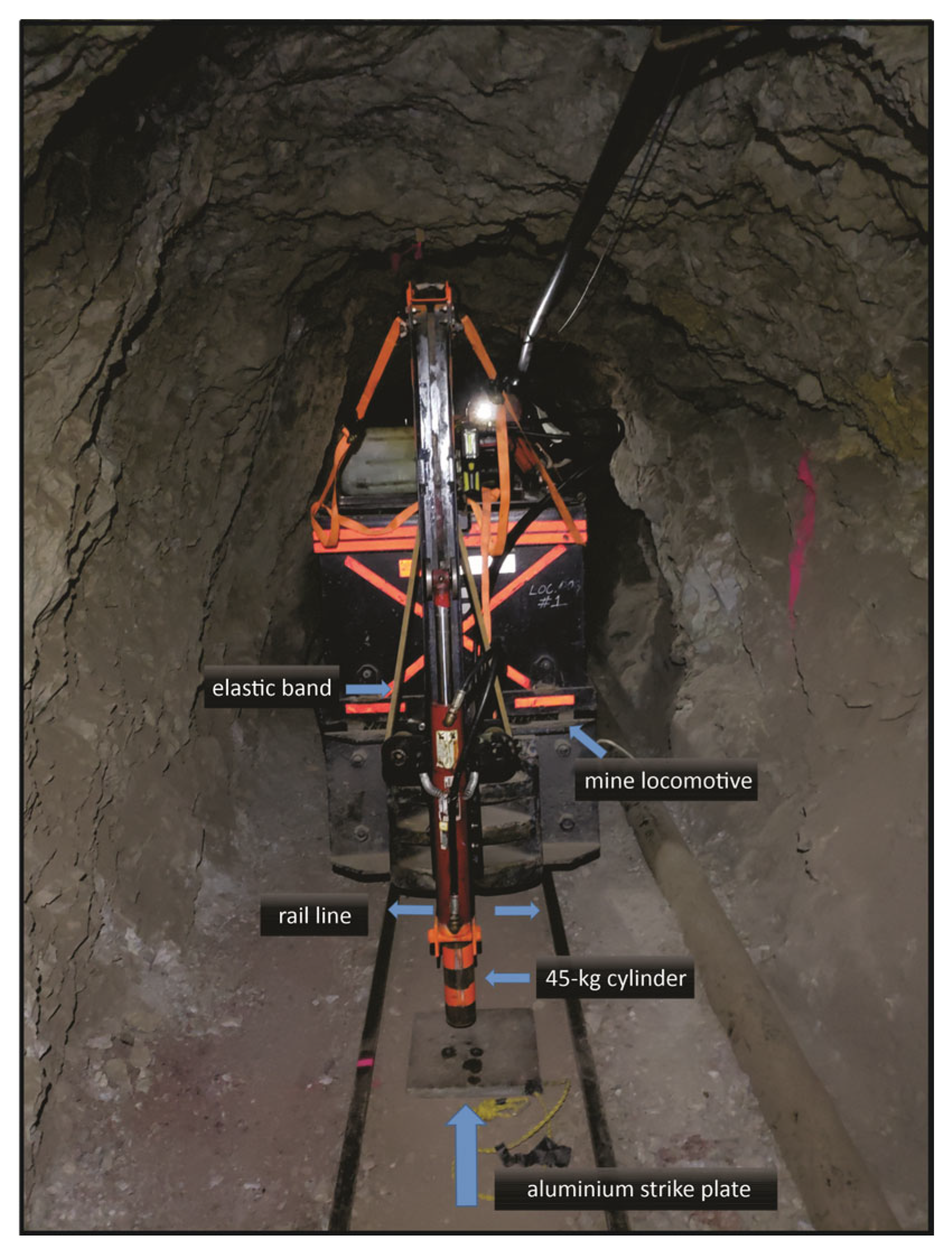
3.1. Seismic Acquisition Methods
3.1.1. Short Test P-Wave High-Resolution CMP and MASW S-Wave Velocity Profile
3.1.2. Extended Conventional P-Wave CMP Profile
3.1.3. HVSR Sounding
3.2. Seismic Data Processing and Modelling Methods
3.2.1. Short Test P-Wave High-Resolution CMP Profile Processing
3.2.2. MASW S-Wave Velocity Profile Modelling
3.2.3. Extended Conventional P-Wave CMP Profile Processing
3.2.4. HVSR Transformation
4. Results
4.1. Short Test P-Wave High-Resolution CMP Profile
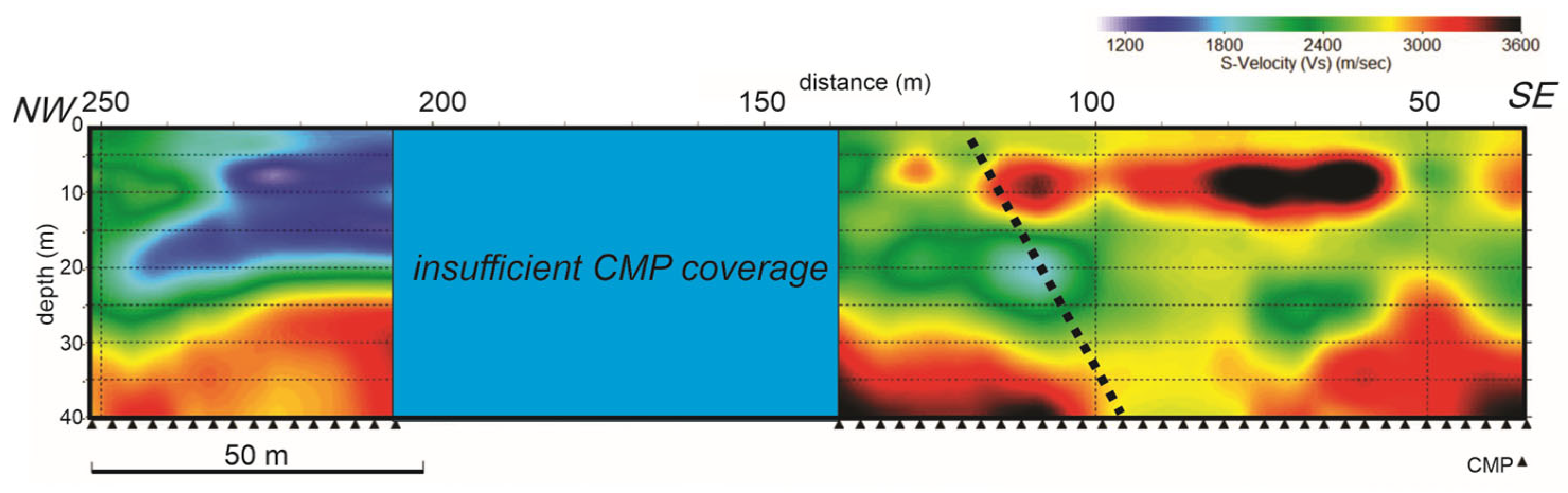
4.2. MASW S-Wave Velocity Profile
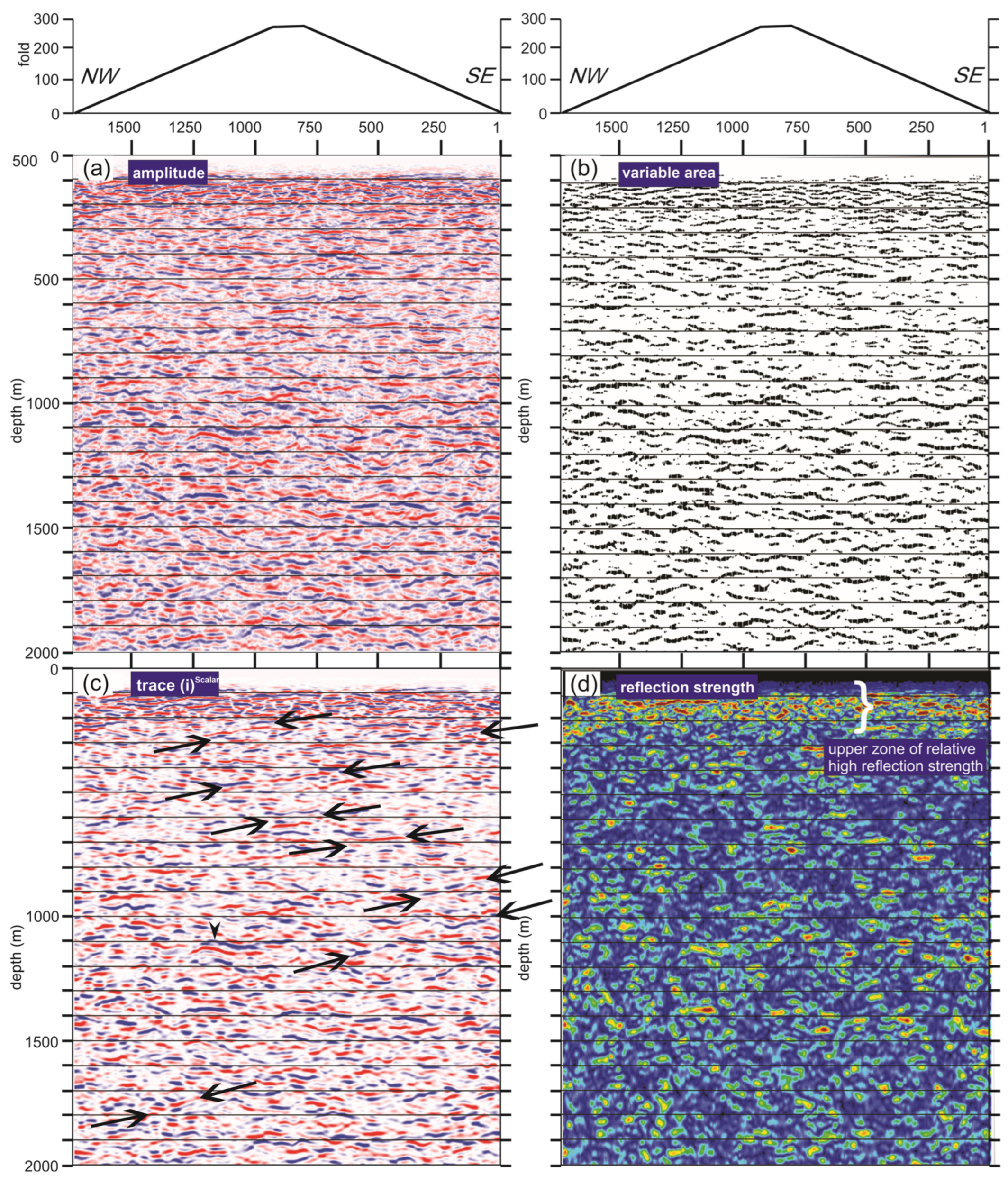
4.3. Extended Conventional P-Wave CMP Profile
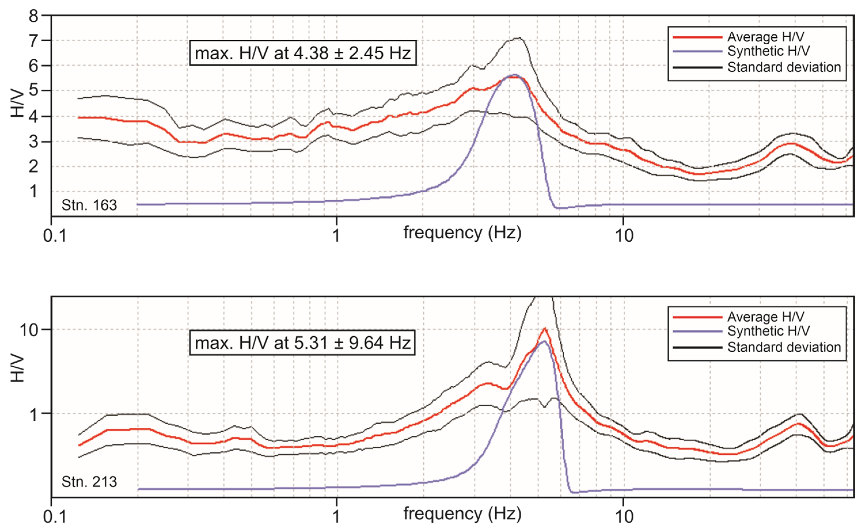
4.4. HVSR Soundings
5. Discussion
6. Conclusions
- The four methods complement each other in terms of resolution, depth penetration, and responsiveness to the elastic parameters of geological targets.
- The HVSR method provides the lowest resolution (i.e., lowest frequency, less than 10 Hz) but can detect fundamental subsurface boundaries with S-wave variations; furthermore, it is the easiest survey by far.
Author Contributions
Funding
Data Availability Statement
Conflicts of Interest
References
- Cardarelli, E.; Marrone, C.; Orlando, L. Evaluation of tunnel stability using integrated geophysical methods. J. Appl. Geophys. 2003, 52, 93–102. [Google Scholar] [CrossRef]
- Malehmir, A.; Durrheim, R.; Bellefleur, G.; Urosevic, M.; Juhlin, C.; White, D.J.; Milkereit, B.; Campbell, G. Seismic methods in mineral exploration and mine planning: A general overview of past and present case histories and a look into the future. Geophysics 2012, 77, WC173–WC190. [Google Scholar] [CrossRef]
- Dehghannejad, M.; Juhlin, C.; Malehmir, A.; Skyttä, P.; Weihed, P. Reflection seismic imaging of the upper crust in the Kristineberg mining area, northern Sweden. J. Appl. Geophys. 2010, 71, 125–136. [Google Scholar] [CrossRef]
- Greenhalgh, S.A.; Mason, I.M.; Sinadinovski, C. In-mine seismic delineation of mineralization and rock structure. Geophysics 2000, 65, 1908–1919. [Google Scholar] [CrossRef]
- Lehmann, B.; Orlowsky, D.; Misiek, R. Exploration of Tunnel Alignment using Geophysical Methods to Increase Safety for Planning and Minimizing Risk. Rock Mech. Rock Eng. 2010, 43, 105–116. [Google Scholar] [CrossRef]
- Ehsan, S.A.; Malehmir, A.; Dehghannejad, M. Re-processing and interpretation of 2D seismic data from the Kristineberg mining area, northern Sweden. J. Appl. Geophys. 2012, 80, 43–55. [Google Scholar] [CrossRef]
- Manzi, M.S.D.; Gibson, M.A.S.; Hein, K.A.A.; King, N.; Durrheim, R.J. Application of 3D seismic techniques to evaluate ore resources in the West Wits Line goldfield and portions of the West Rand goldfield, South Africa. Geophysics 2012, 77, WC163–WC171. [Google Scholar] [CrossRef]
- Manzi, M.; Cooper, G.; Malehmir, A.; Durrheim, R.; Nkosi, Z. Integrated interpretation of 3D seismic data to enhance the detection of the gold-bearing reef: Mponeng Gold mine, Witwatersrand Basin (South Africa). Geophys. Prospect. 2015, 63, 881–902. [Google Scholar] [CrossRef]
- Gendzwill, D.J.; Brehm, R. High-resolution seismic reflections in a potash mine. Geophysics 1993, 58, 741–748. [Google Scholar] [CrossRef]
- Greenhalgh, S.; Mason, I. Seismic imaging with application to mine layout and development. In Proceedings of the Exploration 97: Fourth Decennial International Conference on Mineral Exploration, Toronto, ON, Canada, 14–18 September 1997. [Google Scholar]
- Greenhalgh, S.A.; Bierbaum, S. Underground seismic reflection experiment in a gold mine. Explor. Geophys. 2000, 31, 321–327. [Google Scholar] [CrossRef]
- Yokota, Y.; Yamamota, T.; Shirasagi, S.; Koizumi, Y.; Descour, J.; Kohlhaas, M. Evaluation of geological conditions ahead of TBM tunnel using wireless seismic reflector tracing system. Tunn. Undergr. Space Technol. 2016, 57, 85–90. [Google Scholar] [CrossRef]
- Cheng, J.; Qin, S.; Lu, B.; Wang, B.; Wang, J. The development of seismic-while-mining detection technology in underground coal mines. Coal Geol. Explor. 2019, 47, 2. [Google Scholar] [CrossRef]
- Zhukov, A.; Prigara, A.; Tsarev, R.; Shustkina, I. Method of mine seismic survey for studying geological structure features of Verkhnekamskoye salt deposit. Min. Informational Anal. Bull. 2019, 4, 121–136. [Google Scholar] [CrossRef]
- Nabighian, M.N.; Asten, M.W. Metalliferous mining geophysics—State of the art in the last decade of the 20th century and the beginning of the new millennium. Geophysics 2002, 67, 964–978. [Google Scholar] [CrossRef]
- Luo, X.; Duan, J.; Hatherly, P. Trials of seismic survey for delineation of ore body boundaries. In Proceedings of the Beijing 2014 International Geophysical Conference & Exposition, Beijing, China, 21–24 April 2014. [Google Scholar] [CrossRef]
- Gendzwill, D.J. Underground applications of seismic measurements in a Saskatchewan potash mine. Geophysics 1969, 34, 906–915. [Google Scholar] [CrossRef]
- Istekova, S.A.; Tolybayeva, D.N.; Issayeva, L.D.; Ablessenova, Z.N.; Talassov, M.A. The effectiveness of the use of geophysical research in the underground development of ore deposits. Eng. J. Satbayev Univ. 2024, 146, 24–33. [Google Scholar] [CrossRef]
- Quaternary Fault and Fold Database for the United States. Available online: https://www.usgs.gov/natural-hazards/earthquake-hazards/faults (accessed on 1 August 2019).
- Steven, T.A.; Rowley, P.D.; Cunningham, C.G. Calderas of the Marysvale Volcanic Field, west central Utah. J. Geophys. Res. 1984, 89, 8751–8764. [Google Scholar] [CrossRef]
- Beatty, D.W.; Cunningham, C.G.; Rye, R.O.; Steven, T.A.; Gonzalez-Urien, E. Geology and geochemistry of the Deer Trail Pb-Zn-Ag-Au-Cu manto deposits, Marysvale District, west-central Utah. Econ. Geol. 1986, 18, 1932–1952. [Google Scholar] [CrossRef]
- Kennedy, R.R. Geology between Pine (Bullion) Creek and Tenmile Creek Eastern Tushar Range, Piute County, Utah. Brigh. Young Univ. Res. Stud. Geol. Ser. 1960, 7, 7–8. [Google Scholar]
- Hecker, S. Quaternary Tectonics of Utah with Emphasis on Earthquake-Hazard Characterization; Utah Geological Survey: Salt Lake City, UT, USA, 1993; Volume 127, pp. 1–157.
- Rowley, P.D.; Vice, G.S.; McDonald, R.E.; Anderson, J.J.; Machette, M.N.; Maxwell, D.J.; Ekren, E.B.; Cunningham, C.G.; Steven, T.A.; Wardlaw, B.R. Interim geologic map of the Beaver 30’ x 60’ quadrangle, Beaver, Piute, Iron, and Garfield Counties, Utah. Utah Geol. Surv. Open File Rep. 2005, 454. [Google Scholar] [CrossRef]
- Doll, W.E.; Miller, R.D.; Xia, J. A noninvasive shallow seismic source comparison on the Oak Ridge Reservation, Tennessee. Geophysics 1998, 63, 1122–1479. [Google Scholar] [CrossRef]
- Sheriff, R.E.; Geldart, L.P. Exploration Seismology, 2nd ed.; Cambridge University Press: Cambridge, UK, 1995; pp. 335–342. [Google Scholar] [CrossRef]
- Yilmaz, Ö. Seismic Data Analysis: Processing, Inversion, and Interpretation of Seismic Data; Society of Exploration Geophysicists: Tulsa, OK, USA, 2001; pp. 25–1000. [Google Scholar] [CrossRef]
- Burger, H.B.; Sheehan, A.F.; Jones, C.H. Introduction to Applied Geophysics; Cambridge University Press: Cambridge, UK, 2023; pp. 149–264. [Google Scholar]
- Park, C.B.; Miller, R.D. Roadside passive multi-channel analysis of surface waves (MASW). J. Environ. Eng. Geophys. 2008, 13, 1–11. [Google Scholar] [CrossRef]
- ParkSEIS. Available online: http://www.parkseismic.com/ (accessed on 14 February 2025).
- Miller, R.D.; Xia, J.; Park, C.B.; Ivanov, J.M. Multichannel analysis of surface waves to map bedrock. Lead. Edge 1999, 18, 1393–1396. [Google Scholar] [CrossRef]
- Park, C.B.; Miller, R.D.; Xia, J. Multichannel analysis of surface waves MASW. Geophysics 1999, 64, 800–808. [Google Scholar] [CrossRef]
- Xia, J.; Miller, R.D.; Park, C.B.; Ivanov, J. Construction of 2-D vertical shear-wave velocity field by the multichannel analysis of surface wave technique. In Proceedings of the Symposium on the Application of Geophysics to Engineering and Environmental Problems, Arlington, TX, USA, 20–24 February 2000. [Google Scholar] [CrossRef]
- Robertson, J.D.; Fisher, D.A. Complex seismic trace attributes. Lead. Edge 1988, 7, 22–26. [Google Scholar] [CrossRef]
- Barnes, A.E. Handbook of Poststack Seismic Attributes; Society of Exploration Geophysicists: Tulsa, OK, USA, 2016; pp. 67–72. [Google Scholar] [CrossRef]
- Konno, K.; Ohmachi, T. Ground-motion characteristics estimated from spectral ratio between horizontal and vertical components of microtremor. Bull. Seismol. Soc. Am. 1998, 88, 228–241. [Google Scholar] [CrossRef]
- Arai, H.; Tokimatsu, K. S-wave velocity profiling by inversion of microtremor H/V spectrum. Bull. Seismol. Soc. Am. 2004, 94, 53–63. [Google Scholar] [CrossRef]
- Mahajan, A.K.; Galiana-Merino, J.J.; Lindholm, C.; Arora, B.R.; Mundepi, A.K.; Rai, N.; Chauhan, N. Characterization of the sedimentary cover at the Himalayan foothills using active and passive seismic techniques. J. Appl. Geophys. 2011, 73, 196–206. [Google Scholar] [CrossRef]
- Owers, M.C.; Meyers, J.; Siggs, B.; Shackleton, M. Passive seismic surveying for depth to base of paleochannel mapping at Lake Wells, Western Australia. ASEG Ext. Abstr. 2016, 1, 1–9. [Google Scholar] [CrossRef]
- Nelson, S.; McBride, J. Application of HVSR to estimating thickness of laterite weathering profiles in basalt. Earth Surf. Process. Landf. 2019, 44, 1365–1376. [Google Scholar] [CrossRef]
- Mi, B.; Hu, Y.; Jianghai, X.; Socco, L.V. Estimation of horizontal-to-vertical spectral ratios (ellipticity) of Rayleigh waves from multistation active-seismic records. Geophysics 2019, 84, EN81–EN92. [Google Scholar] [CrossRef]
- Thabet, M. Site-specific relationships between bedrock depth and HVSR fundamental resonance frequency using KiK-NET data from Japan. Pure Appl. Geophys. 2019, 176, 4809–4831. [Google Scholar] [CrossRef]
- Castellaro, S.; Mulargia, F.; Bianconi, L. Passive seismic stratigraphy: A new efficient, fast and economic technique. Geol. Tec. Ambient. 2005, 3, 76–102. [Google Scholar]
- Lu, X.; Wang, W.; Yang, C.; Hu, X.; Liao, X.; Fu, Z. Exploring the influence of seismic source and improvement methods on tunnel seismic prediction. Lithosphere 2024, 2024, 1–14. [Google Scholar] [CrossRef]
- Li, S.; Liu, B.; Xu, X.; Nie, L.; Liu, Z.; Song, J.; Sun, H.; Chen, L.; Fan, K. An overview of ahead geological prospecting in tunneling. Tunn. Undergr. Space Technol. 2017, 63, 69–94. [Google Scholar] [CrossRef]


Disclaimer/Publisher’s Note: The statements, opinions and data contained in all publications are solely those of the individual author(s) and contributor(s) and not of MDPI and/or the editor(s). MDPI and/or the editor(s) disclaim responsibility for any injury to people or property resulting from any ideas, methods, instructions or products referred to in the content. |
© 2025 by the authors. Licensee MDPI, Basel, Switzerland. This article is an open access article distributed under the terms and conditions of the Creative Commons Attribution (CC BY) license (https://creativecommons.org/licenses/by/4.0/).
Share and Cite
McBride, J.H.; Lambeck, L.; Rey, K.A.; Nelson, S.T.; Keach, R.W. Experimental Seismic Surveying in a Historic Underground Metals Mine. Geosciences 2025, 15, 221. https://doi.org/10.3390/geosciences15060221
McBride JH, Lambeck L, Rey KA, Nelson ST, Keach RW. Experimental Seismic Surveying in a Historic Underground Metals Mine. Geosciences. 2025; 15(6):221. https://doi.org/10.3390/geosciences15060221
Chicago/Turabian StyleMcBride, John H., Lex Lambeck, Kevin A. Rey, Stephen T. Nelson, and R. William Keach. 2025. "Experimental Seismic Surveying in a Historic Underground Metals Mine" Geosciences 15, no. 6: 221. https://doi.org/10.3390/geosciences15060221
APA StyleMcBride, J. H., Lambeck, L., Rey, K. A., Nelson, S. T., & Keach, R. W. (2025). Experimental Seismic Surveying in a Historic Underground Metals Mine. Geosciences, 15(6), 221. https://doi.org/10.3390/geosciences15060221