Review of Correlations Between Soil Electrical Resistivity and Geotechnical Properties

Abstract

This review presents a comprehensive synthesis of existing studies on the correlations between soil electrical resistivity and fundamental geotechnical properties, with the aim of improving the applicability of resistivity testing in geotechnical engineering. Based on both laboratory and field research, the analysis highlights moisture content as the most influential factor inversely affecting resistivity, followed by plasticity index, clay content, and dry unit weight. Statistical approaches—including regression analysis and Spearman’s rank correlation—and artificial neural networks (ANNs) were evaluated for their effectiveness in modeling these nonlinear relationships. ANNs demonstrated superior predictive performance, particularly in heterogeneous and fine-grained soils. The review also examines the influence of temperature and salinity, emphasizing the need for multivariable models for robust interpretation. While resistivity testing shows great potential for non-destructive soil classification and compaction assessment, limitations related to soil type specificity, environmental variability, and model generalizability are noted. This work provides an important foundation for the development of data-driven, non-invasive techniques for subsurface characterization and outlines directions for future research, including field validation and hybrid modeling.

1. Introduction

1.1. Background and Significance

The correlation between soil electrical resistivity and geotechnical properties has garnered substantial attention in recent decades, particularly due to the value of resistivity measurements in geotechnical site characterization and subsurface profiling. Electrical resistivity testing is a non-destructive, cost-effective technique that enables the indirect estimation of key soil properties, providing insight into both mechanical and hydraulic behavior relevant to a range of civil and environmental engineering applications [1,2,3,4,5,6,7].

Numerous studies have shown that geotechnical parameters—particularly moisture content, plasticity index (PI), and soil density measures such as dry unit weight, bulk density, and unit weight—have a significant influence on soil resistivity. Moisture content is typically the most dominant factor, showing a strong inverse relationship with resistivity due to enhanced ionic conduction. Plasticity index also affects resistivity, especially in fine-grained soils, as it relates to mineralogy and surface conduction behavior. These effects are explored in greater detail in Section 4.1 and Section 4.2. Among these, moisture content is consistently identified as the most dominant factor, showing a nonlinear inverse relationship with resistivity: as water content increases, ionic mobility improves, and continuous conduction pathways form, leading to reduced resistivity values [8,9,10,11]. Similarly, changes in soil density affect electrical conduction by altering the degree of saturation, void ratio, and interparticle contact, all of which control current flow through the soil matrix [12,13,14].

In addition to physical and hydraulic influences, mineralogical characteristics also play a crucial role. Higher clay content and plasticity index are generally associated with lower resistivity, particularly under unsaturated conditions, due to mechanisms such as surface conduction, electrical double layers, and the presence of adsorbed water. However, these relationships are often nonlinear, site-dependent, and affected by external factors such as pore fluid chemistry, temperature, and soil stratification. This complexity necessitates a multivariable modeling approach to more accurately predict and interpret resistivity behavior across different soil types and environmental conditions [15,16,17,18,19].

While empirical studies have demonstrated general trends, traditional modeling techniques often struggle to capture the inherent heterogeneity and nonlinearity of natural soils. To address these limitations, recent research has explored the use of computational methods, including regression analysis and artificial neural networks (ANNs). Regression offers structured and interpretable relationships, while ANNs are particularly effective in identifying and modeling complex, nonlinear patterns in data without requiring predefined assumptions [20,21,22].

Given the diversity of soil types and field conditions, there remains a critical need for improved predictive models that can integrate these variable influences and enhance the interpretability of electrical resistivity data. This review aims to investigate and quantify the relationships between resistivity and key geotechnical properties—specifically, moisture content, plasticity index, unit weight, dry density, bulk density, and clay content—through the application of both statistical regression and ANN-based modeling techniques. By combining insights from the prior literature with data-driven model development, this work contributes to more accurate resistivity-based soil assessments and advances the practical use of geotechnical data in subsurface investigations.

Despite numerous studies examining the general trends between electrical resistivity and geotechnical parameters, a significant gap remains in the integration of multiple influencing factors within a unified modeling framework. Most existing models are limited to single-variable correlations or are constrained by specific soil types, lacking generalizability across varied environmental and geological conditions. Furthermore, the nonlinear and site-specific nature of these relationships often challenges the accuracy and interpretability of conventional regression models. As such, there is a need for comprehensive studies that synthesize multivariable interactions using both statistical and advanced machine learning approaches to improve predictive accuracy and practical applicability. This review addresses this gap by systematically analyzing and modeling the relationships between resistivity and key geotechnical properties using both regression and artificial neural network (ANN) techniques, with the goal of enhancing the reliability of non-invasive soil assessments across diverse conditions.

1.2. Objectives and Scope of the Study

The objective of this review is to quantitatively evaluate the relationship between soil electrical resistivity and key geotechnical parameters under various soil conditions. Specifically, the study aims to achieve the following:

• Develop predictive models linking resistivity with geotechnical parameters such as moisture content, plasticity index, unit weight, dry density, bulk density, and clay content;
• Assess the influence of each parameter on resistivity behavior using both statistical and machine learning techniques;
• Compare model performance across different soil types and stratified conditions to identify patterns in resistivity variation;
• Enhance the interpretability of resistivity data to support non-invasive soil assessment in geotechnical engineering practice.

The scope of this review includes both laboratory-controlled and field-collected data, covering a variety of soil textures and compositions. Analyses consider both individual and combined effects of geotechnical parameters, using correlation coefficients, regression functions, and ANNs to capture linear and nonlinear behaviors. Particular emphasis is placed on the multivariable interactions that affect resistivity in stratified or moisture-variable soils.

1.3. Structure of the Paper

This paper is structured to progressively address the theoretical foundation, data modeling, and practical implications of resistivity–soil property correlations.

Section 2 introduces the basic principles of electrical resistivity in soils, covering the theoretical background. This section provides the scientific basis for understanding how soil resistivity varies with different parameters.

Section 3 details the statistical methods and computational frameworks used in this review, including regression analysis, Spearman’s rank correlation, and ANN modeling.

Section 4 presents the results and discussion, organized by geotechnical parameter: moisture content, plasticity index, clay content, temperature, unit weight, and density. Subsections examine each parameter’s influence on resistivity and the predictive performance of the proposed models.

Section 5 presents the discussion, interpreting the correlation results and highlighting their implications for geotechnical applications and substation design. It also addresses the limitations of the study and outlines directions for future research.

Section 6 presents the conclusions, summarizing the key findings of the review and reaffirming the most influential geotechnical parameters affecting soil resistivity.

This structure provides a comprehensive framework for understanding and modeling the relationship between electrical resistivity and geotechnical properties, supporting improved applications in site investigation and soil classification.

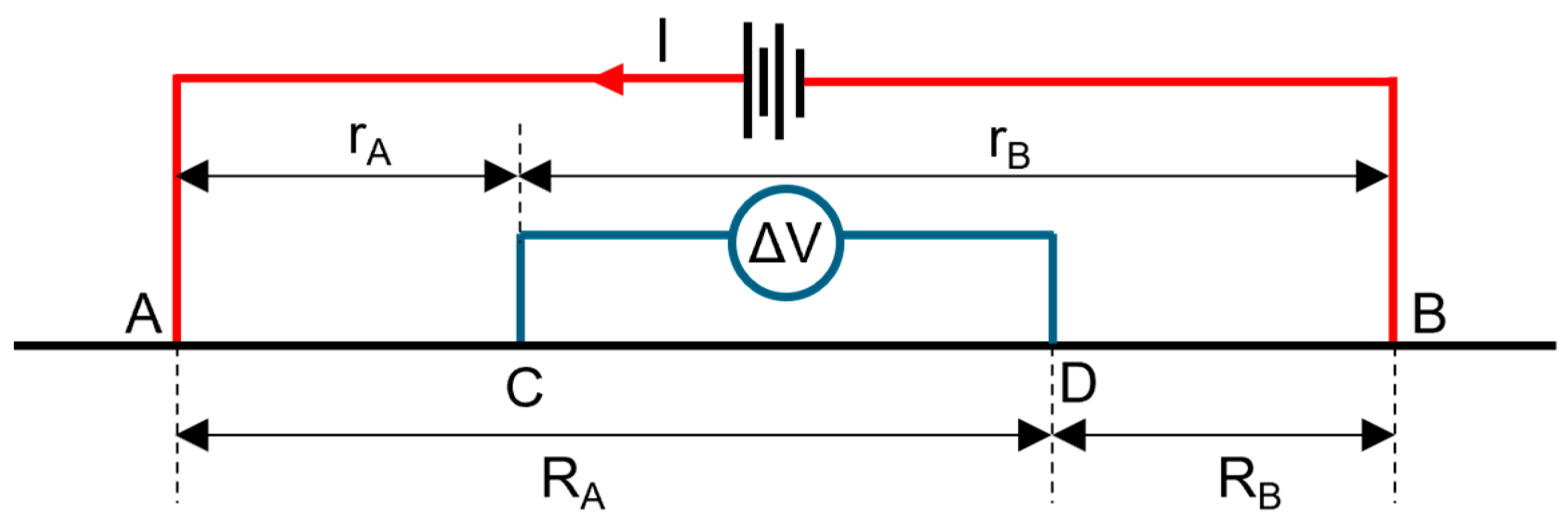
2. Fundamentals of Electrical Resistivity in Soils

Principles of Electrical Resistivity

Electrical techniques used in geophysical surveys are some of the most critical methodologies that provide in-depth insight into the resistivity distribution of the subsurface, which is essential for the effective design of grounding systems. These methods involve the application of artificially generated electric currents into the ground and then the precise measurement of the resulting potential differences at various points. The patterns of these potential differences are meticulously analyzed to reveal the nature and structure of subsurface heterogeneities and their associated electrical properties. Such detailed information is essential for understanding the complex subsurface environment and optimizing grounding system performance [4,23].

In a homogeneous earth model, electric current flows radially outward from the source, creating a uniform distribution across the surface, often referred to as an equipotential surface. This uniformity implies that the current distribution remains the same at every point on this surface. However, the pattern of current flow lines is influenced by the properties of the medium being examined, with these lines becoming more concentrated in regions of higher conductivity. For a simple body, as shown in Figure 1, the resistivity of the medium can be characterized by the following Equation (1):

$$R=\rho \left({\displaystyle \frac{L}{A}}\right)$$

(1)

where $R$ is the electrical resistance measured in ohms, $\rho$ is the resistivity of the material in ohm-meters, $A$ is the cross-sectional area in square meters, and $L$ is the length of the cylindrical body in meters. The electrical resistance $R$ of a cylindrical conductor can be determined using Ohm’s law as formulated in Equation (2), written as follows:

$$R={\displaystyle \frac{V}{I}}$$

(2)

A current, denoted as $I$, is introduced into the cylindrical element, resulting in a potential drop, denoted as $-\delta V$, across the two ends of the cylinder. According to Ohm’s law, this potential difference, current, and resistance are related by the expression $-\delta V=\delta R·I$. Here, the incremental resistance $\delta R$ is defined by the relationship $\delta R={\displaystyle \frac{\delta L}{\delta A}}$. By substituting these expressions into the equation we obtain Equation (3), written as follows:

$${\displaystyle \frac{\delta V}{\delta L}}=-\rho \left({\displaystyle \frac{I}{\delta A}}\right)=-\rho J$$

(3)

where ${\displaystyle \frac{\delta V}{\delta L}}$ is the potential gradient across the element in volts per meter, $J$ is the current density in amperes per square meter.

In a homogeneous and isotropic half-space, where the properties of the medium are uniform in all directions, the electrical equipotential surfaces assume a hemispherical shape when current electrodes are positioned at the soil surface [4,5,6,7]. Under these conditions, the current density, denoted as $J$ and measured in amperes per square meter, must be determined for all radial directions emanating from the source. The calculation of the current density is governed by the following relationship in Equation (4):

$$J={\displaystyle \frac{I}{2\pi r^2}}$$

(4)

where $I$ is the electric current in amperes and $2\pi r^2$ is the surface area of a hemispherical sphere with radius $r$ in square meters. Based on the given equation, the potential gradient corresponding to this current density can be expressed as Equation (5), written as follows:

$${\displaystyle \frac{\delta V}{\delta R}}=-\rho J=-{\displaystyle \frac{\rho I}{2\pi r^2}}$$

(5)

The potential $V_r$ at distance $r$ is then obtained by integration as Equation (6):

$$V_r=\int \partial V=-\int {\displaystyle \frac{\rho I\partial r}{2\pi r^2}}={\displaystyle \frac{\rho I}{2\pi r}}$$

(6)

The integration constant is determined to be zero, since the potential $V_r$ is zero as the radial distance $r$ approaches infinity.

According to Kearey et al. (2002) [4], when the current sink is located at a finite distance from the current source, as shown in Figure 2, point $A$ denotes the current source electrode, while point $B$ represents the current sink electrode. Points $C$ and $D$ are potential electrodes used to measure the voltage difference ($∆V$) between them. The potential $V_C$ at an internal electrode $C$ is determined by the combined contributions of the potentials $V_A$ and $V_B$ due to the current injected at point $A$ and withdrawn at point $B$, respectively, as Equation (7) [4].

$$V_C=V_A-V_B$$

(7)

Substitute Equation (6) into Equation (7) as Equations (8) and (9).

$$V_C={\displaystyle \frac{\rho I}{2\pi }}\left({\displaystyle \frac{1}{r_A}}-{\displaystyle \frac{1}{r_B}}\right)$$

(8)

$$V_D={\displaystyle \frac{\rho I}{2\pi }}\left({\displaystyle \frac{1}{R_A}}-{\displaystyle \frac{1}{R_B}}\right)$$

(9)

Monitoring absolute potentials presents significant challenges; therefore, the potential difference $∆V$ between electrodes $C$ and $D$ is typically measured instead. ∆V can then be calculated using Equation (10).

$$∆V=V_C-V_D={\displaystyle \frac{\rho I}{2\pi }}\left\{\left({\displaystyle \frac{1}{r_A}}-{\displaystyle \frac{1}{r_B}}\right)-\left({\displaystyle \frac{1}{R_A}}-{\displaystyle \frac{1}{R_B}}\right)\right\}$$

(10)

In this way, either Equations (11) or (12) is derived.

$$\rho ={\displaystyle \frac{∆V}{I}}\mathsf{\bullet }{\displaystyle \frac{2\pi }{\left\{\left(\frac{1}{r_A}-\frac{1}{r_B}\right)-\left(\frac{1}{R_A}-\frac{1}{R_B}\right)\right\}}}$$

(11)

$$\rho =K{\displaystyle \frac{∆V}{I}}$$

(12)

where $K$ is a geometric coefficient related to the specific configuration of the electrodes. The inverse of this coefficient, $1/K$, is called the intensity coefficient. A higher intensity coefficient indicates that the electrode array has superior noise immunity and a higher signal-to-noise ratio. Among various electrode configurations, the Wenner probe [10] arrays have the lowest geometric factor, $K=2\pi a$, which means that these configurations provide the strongest resistance to external disturbances due to their maximum intensity coefficient, where a is the distance between the electrodes [2,8].

Liu and Kitanidis (2013) [11], along with Glover (2009) [12], highlight that Archie’s Law, formulated by Archie in 1942, remains the most widely used method for analyzing the properties of porous materials. This approach establishes a relationship between electrical resistivity and factors such as porosity and moisture content. Archie’s equation, which encapsulates this relationship, can be expressed as Equation (13).

$$F={\displaystyle \frac{R_b}{R_w}}={\theta }^{-m}$$

(13)

where $F$ is the formation resistivity factor, $R_b$ is the resistivity of the bulk rock in ohms, $R_w$ is the resistivity of the formation fluid in ohms, and $\theta$ is the porosity of the material. The parameter $m$, known as the cementation exponent, can be determined as the slope of a log-log plot of $F$ versus $\theta$.

In addition to open pore spaces, the transport of fluids within a porous medium is also critical. The soil grains create obstacles that cause particles to follow a longer, more tortuous path than a direct line. Consequently, tortuosity has been incorporated into the generalized form of Archie’s law with Equation (14) as proposed by Revil et al. (1998) [13].

$$F={\displaystyle \frac{R_b}{R_w}}={\displaystyle \frac{\mathrm{a}}{{\theta }^m}}$$

(14)

Electrical resistivity testing is typically conducted using a direct current (DC) or low-frequency alternating current (AC) resistivity meter connected to four electrodes arranged in standard configurations, most commonly Wenner or Schlumberger arrays. These setups involve two outer electrodes that inject current into the ground and two inner electrodes that measure the resulting voltage difference. The apparent resistivity is then calculated based on Ohm’s law and a configuration-specific geometric factor. By increasing the spacing between electrodes, the method can probe progressively deeper soil layers. The effective depth of investigation is generally considered to be approximately one-quarter to one-half of the total electrode spacing. For instance, an electrode spacing of 1 m typically corresponds to an investigation depth of 0.25 to 0.5 m. Consequently, the representative volume of soil assessed depends on the array geometry and electrode spacing, typically ranging from several cubic decimeters to a few cubic meters. This allows for bulk characterization of subsurface properties in a non-destructive manner. Field deployment may involve site preparation, ensuring good electrode contact with the soil, and multiple readings to reduce measurement variability [24].

3. Correlation Analysis

Several studies have investigated the relationship between electrical resistivity and geotechnical properties [25,26,27]. Various mathematical approaches have been employed to analyze these relationships, with regression analysis and artificial neural networks (ANNs) being the most commonly used methods. The theoretical foundations of these methods are described in this section.

To accurately quantify the error associated with nonlinear regression, the quality and effectiveness of the fitted data model are evaluated using the coefficient of determination, commonly referred to as $R^2$. This coefficient, calculated using Equation (15), serves as a critical measure of how well the model explains the variability of the response data around its meaning.

$$R^2=1-{\displaystyle \frac{\mathbf{\sum }{\left(y_i-{\widehat{y}}_i\right)}^2}{\mathbf{\sum }{\left(y_i-{\overline{y}}_i\right)}^2}}$$

(15)

where $y_i$ is the tested data, ${\widehat{y}}_i$ is the least squares prediction, and ${\overline{y}}_i$ is the mean of the statistical data. For an ideal or perfect fit, the coefficient of determination ($R^2$) is equal to 1, indicating that the regression line explains 100% of the variability observed in the data. Conversely, if the coefficient ($R^2$) is 0, it means that the regression model does not explain any variability in the data [27].

The strength of association between two variables can be assessed using Spearman’s rank correlation coefficient, which measures the relationship based on a monotonic function. Unlike Pearson’s correlation, Spearman’s method is non-parametric and does not assume a specific distribution of the data. It also does not require the designation of dependent or independent variables, although this can be performed when relevant. Spearman’s coefficient (rₛ) is calculated using the ranks of the data rather than their actual values, making it suitable for variables measured on an ordinal scale. By replacing categorical values with their ranks, rₛ quantifies how closely two sets of rankings agree with each other, thus indicating the degree of correlation between the variables [28]. Spearman’s coefficient (rₛ) can be calculated as Equation (16), written as follows:

$$r_s=1-{\displaystyle \frac{6\mathbf{\sum }{d}_i^2}{n\left(n^2-1\right)}}$$

(16)

where $n$ is number of pairs and $d_i$ is the difference between ranks ($x_i-y_i$). rₛ can be interpreted as shown in

Table 1. The interpretation of Spearman’s coefficient (rₛ).

rₛ Value	Strength of Association
+1	Perfect positive
−1	Perfect negative
0	No association
0.1 to 0.3 or −0.1 to −0.3	Weak
0.4 to 0.6 or −0.4 to −0.6	Moderate
0.7 to 0.9 or −0.7 to −0.9	Strong

.

3.1. Regression Analysis

Regression analysis is a fundamental statistical technique that is widely used to evaluate associations within data sets and to determine the relative influence of individual variables [27,29,30,31,32]. The primary mathematics for a simple linear regression is expressed as Equation (17), written as follows:

$$y={\beta }_0+{\beta }_{1}x+\epsilon$$

(17)

where $x$ is the independent variable, $y$ is the dependent variable, ${\beta }_0$ is the intercept when x is 0, ${\beta }_1$ is the regression coefficient that is an unknown parameter, and e is a statistical error.

In the case where the dataset consists of n sets of observations ($x_1$, $x_2$, $\cdots$, $x_i$), which represent a random sample, the relationship among variables can be described using a multiple linear regression model. This model is mathematically expressed as Equation (18), written as follows:

$$y={\beta }_0+{\beta }_1{x}_1+{\beta }_2{x}_2+\cdots +{\beta }_i{x}_i+\epsilon$$

(18)

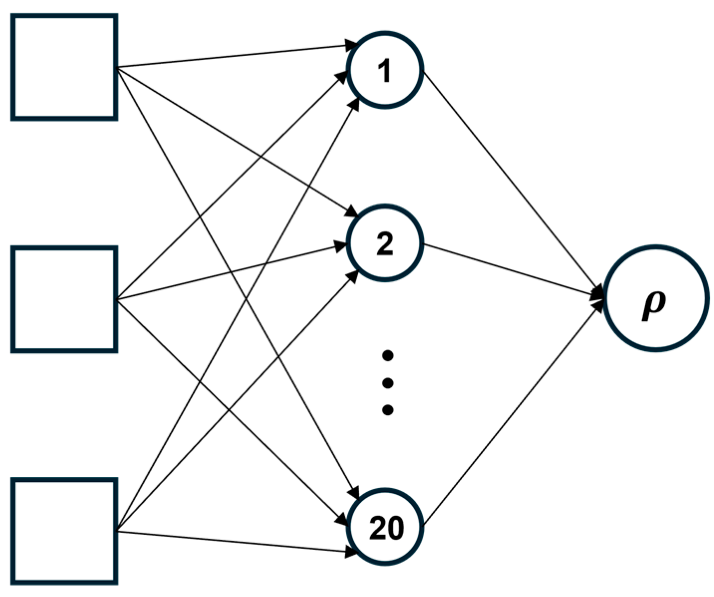
3.2. Artificial Neural Networks

Artificial neural networks (ANNs) are computational models that emulate the structure and function of the human brain. Unlike conventional algorithmic approaches that rely on sequential, rule-based logic, ANNs are capable of learning from data by identifying and modeling complex, nonlinear relationships. This characteristic renders ANNs particularly effective in geotechnical engineering applications, such as the prediction of electrical resistivity, where subsurface properties exhibit intricate interdependencies that are often difficult to capture using traditional analytical methods.

ANNs are commonly implemented as multilayer feedforward networks, comprising an input layer, one or more hidden layers, and an output layer. These layers are composed of interconnected processing units, or neurons, each associated with weights and biases that determine the strength and behavior of the connections. During the training phase, the network iteratively adjusts these parameters to minimize the discrepancy between predicted outputs and actual target values. This optimization is typically performed using backpropagation and continues over multiple training cycles, known as epochs. In a fully connected architecture, each neuron in a given layer is connected to every neuron in the subsequent layer, allowing the network to learn from complex and high-dimensional datasets. The general structure of a multilayer feedforward neural network is commonly illustrated to emphasize these interconnections and the flow of information throughout the model (Figure 3) [33,34,35,36].

Recent studies have demonstrated the effectiveness of deep learning algorithms in modeling the nonlinear relationships between electrical resistivity and geotechnical parameters. Zamanian et al. (2024) [37], for example, successfully applied a deep neural network to predict geotechnical properties from resistivity data, achieving higher accuracy than conventional machine learning models. Building on these advancements, this study incorporates both regression and artificial neural network (ANN) techniques to evaluate the predictive capabilities of data-driven approaches in the context of soil resistivity modeling. Following the methodology of Siddiqui et al. (2014) [38], the ANN model used in this study was constructed with a single hidden layer comprising ten neurons. A sigmoid activation function was applied in the hidden layer, while a linear activation function was used in the output layer to support continuous variable prediction. Prior to training, all input variables were normalized using min–max scaling to a [0,1] range. To mitigate overfitting, early stopping based on validation error was implemented, and L2 regularization was applied to manage model complexity.

4. Influence of Soil Properties on Electrical Resistivity

4.1. Effect of Moisture Content

Numerous studies have investigated the phenomenon of electrical resistivity in soils and its relationship with various soil properties. Researchers have successfully established correlations between soil water content and electrical resistivity (

Table 2. Summary of equation models for the relationship between electrical resistivity and water content of soil.

Author(s)	Soil Type	Findings	${\mathit{R}}^2$	Limitation
Cosenza et al., 2006 [14]	Alluvial deposit soil(Coarese dry soil and fine wet soil)	$\rho =1.187w^{-2.444}$	0.8210	The correlation was limited by data collection and interpolation errors, as the water content samples were collected from only two boreholes, and the electrical resistivity values were interpolated from 2D inversion data to match the depths of the geotechnical tests.
Ozcep et al., 2009 [24]	Sandy soil	$w=49.21{\mathrm{e}}^{-0.017\rho }$	0.7859	The study is limited by the use of only certain soil types and by not controlling parameters such as salinity, which significantly influence electrical resistivity.
Ozcep et al., 2010 [25]	Sandy soil	AI, including ANNs and Fuzzy Logic systems, were employed to predict soil water content using electrical resistivity as the input parameter.	-	The models were based solely on sandy soils, lacked multivariate analysis, and were not validated with independent or external data.
Kibria & Hossain 2012 [21]	Highly plastic clay	$\rho =16.366{\left[{\displaystyle \frac{w\gamma }{1+w}}\right]}^{-1.148}$	0.6400	The study is limited to a specific soil type, which is highly plastic clay.
Abidin et al., 2013 [29]	Loose clayey silt	$w=109.98{\rho }^{-0.268}$	0.8927	The study is limited by its focus on a single soil type and the absence of validation using real field data.
	Compacted clayey silt	$w=121.88{\rho }^{-0.363}$	0.8853
Siddiqui & Osman 2013 [15]	Silty sand	$w=0.6261{\rho }^{-0.156}$	0.2554	The study focuses on sandy and silty sand soils, with weak correlation in silty sand. The site-specific models require recalibration for broader application.
	Sandy soil	$w=0.1954e^{-\left(2\times {10}^{-4}\right)\rho }$	0.5100
	All soil sample	$w=0.9756{\rho }^{-0.263}$	0.5625
Siddiqui et al., 2014 [38]	Silty sand and sandy soil	ANNs was employed to predict soil water content using electrical resistivity as the input parameter.	0.2990	The study focuses on sandy and silty sand soils with weak correlations, using a small dataset that may reduce statistical reliability and increase overfitting risk.
Hazreek et al., 2015 [16]	Clayey silt	$w=109.98{\rho }^{-0.268}$	0.8927	The study lacks field validation, and the broad, overlapping resistivity ranges limit its classification accuracy.
	Silty sand	$w=638.8{\rho }^{-0.418}$	0.5643
Asif et al., 2016 [18]	Clayey sand	$w=-3.78\ln \rho +25.16$	0.964	The correlation is limited due to data being collected from only one specific site.
Kazmi et al., 2016 [39]	Silty sand and sandy soil	$w=106.65{\rho }_{lab}^{-0.271}$	0.5954	The correlation is limited by single-site data collection, lack of external validation, and only moderate predictive accuracy.
	Silty sand and sandy soil	$w=92.862{\rho }_{field}^{-0.261}$	0.5442
Lin et al., 2017 [19]	Marine clay	$w=427.8{\rho }^{-1.13}$	0.9300	Spearman’s rank correlation captures only monotonic trends, not precise predictive accuracy, like $R^2$. The model is based on site-specific Jiangsu marine clay and lacks validation with external data, raising the risk of overfitting to local conditions.
Oborie and Akana 2020 [40]	Fined grained soil	$\rho =-0.908w+103.5$	0.2530	The correlation is limited by the use of simple linear models to represent inherently nonlinear trends, resulting in only moderate to weak correlation strengths.
	Sandy soil	$\rho =-6.918w+339.3$	0.0364
	Poorly graded sands	$\rho =-19.24w+728.0$	0.5810
	All soil samples	$\rho =-7.593w+384.8$	0.3860
Jusoh et al., 2022 [17]	Clayey sand	$w=216.05{\rho }^{-0.36}$	0.8784	The correlation is limited by single-site data collection and lack of external validation.
Sangprasat et al., 2024 [20]	Clayey silt and silty clay	The inverse relationship between resistivity and water content was strong within specific soil types but became weak when all soil samples were analyzed together.	-	The correlation is limited by all tested samples being fine-grained cohesive soils. The correlation equations are not reported by the original authors.

), showing that soil resistivity decreases with increasing water content due to a rise in hydrated ions and enhanced conduction pathways.

In sandy soils, stronger and more consistent correlations between resistivity and moisture content are observed, primarily due to their low water retention and large, uniform pore spaces. Kazmi et al. (2016) [39] reported stronger correlations in sandy soils compared to silty ones. In their study, sandy soils exhibited power–law relationships with moderate correlation strength. Similarly, Siddiqui and Osman (2013) [15] found a better fit for sandy soils than for silty sand.

Silty and silty sandy soils demonstrate weaker correlations due to mixed grain sizes and more variable pore distributions. Kazmi et al. (2016) [39] and Oborie and Akana (2020) [40] reported lower correlation coefficients for silty sand, noting diminished sensitivity of resistivity at higher moisture levels. Abidin et al. (2013) [29] proposed a power–law correlation indicating a strong inverse relationship in clay–silt under controlled laboratory conditions.

Clay soils exhibit more complex behavior due to surface conduction mechanisms, adsorbed water, and double-layer effects. Cosenza et al. (2009) [41] provided theoretical support through a structural model, emphasizing the role of the diffuse double layer and water continuity in resistivity behavior. Kibria and Hossain (2012) [21] observed significant resistivity changes up to 20% moisture content, beyond which the values plateaued, suggesting a saturation threshold.

Moreover, Hillel (2003) [42] found that at low water content, the limited mobility of electrical charges—due to water being tightly bound in soil films—results in increased resistivity. Soil resistivity generally increases sharply when moisture content falls below 15% of the total soil weight. Soil moisture content is influenced by grain size, compaction, and variability. When the moisture content exceeds 22%, further changes in resistivity become minimal [1,43]. Lin et al. (2017) [19] reported a strong negative Spearman correlation (r_s = −0.958) between resistivity and moisture content in marine clays, confirming moisture as the most influential geotechnical parameter.

The relationship, however, is typically nonlinear—most often expressed through power–law, logarithmic, or exponential functions. The strength and form of the correlation vary depending on the quantity, type, and concentration of dissolved ions in water. Kizlo and Kanbergs (2009) [44] measured the resistivity of water types, highlighting the influence of dissolved ions. Distilled water exhibits a high resistivity of 50,000 Ω·m, while rainwater (200 Ω·m) is more conductive due to the presence of dissolved ions. Tap water (70 Ω·m) and well water (20–70 Ω·m) have even lower resistivity due to dissolved minerals. In contrast, mixtures of river water and seawater (2 Ω·m) and seawater (0.15–0.3 Ω·m) exhibit significantly lower resistivity due to high salinity, making them highly conductive.

4.2. Impact of Plasticity Index

The relationship between electrical resistivity and plasticity index (PI) varies significantly with soil type, but a general inverse trend is consistently observed across previous studies, as shown in Table 3. For silty sand soil, multiple studies report moderate correlations between PI and resistivity. Osman et al. (2013) [45] found that silty sand samples with intermediate plasticity indices (1.41% to 26.27%) exhibited a strong inverse correlation with laboratory resistivity (R² = 0.501) and a moderate correlation with field resistivity (R² = 0.361). Similarly, Siddiqui and Osman (2013) [15] reported an exponential relationship in silty sands with R² = 0.15, while ANN modeling further improved prediction accuracy to R² = 0.56. In contrast, clayey silt soils showed slightly better statistical relationships, with Oborie and Akana (2020) [40] reporting R² values of 0.45 for clays and 0.52 for clayey sands, supporting the view that finer-grained soils with higher PI tend to exhibit lower resistivity due to enhanced ionic conduction in pore fluids.

For marine clays, which are characterized by high water content and often higher PI values, the relationship is more complex. Lin et al. (2017) [19] demonstrated a very strong inverse correlation between resistivity and PI using Spearman’s rank test (r_s = −0.901), suggesting that PI can serve as a reliable proxy for interpreting resistivity patterns in such deposits. Zhang et al. (2018) [46] further refined this observation, noting that in low-plasticity marine clays (PI < 10%), resistivity decreases as PI increases, but for PI > 10%, resistivity values stabilize around 8 Ω·m, indicating a threshold beyond which PI exerts minimal influence. This plateau effect is attributed to the saturation of conduction pathways in highly plastic and fine-grained clays, where additional clay content does not significantly alter electrical behavior. These findings are consistent with earlier conclusions by Long et al. (2012) [47], who highlighted that resistivity in marine clays is predominantly influenced by salt content and clay mineralogy rather than PI alone.

In sandy soils, the correlation between PI and resistivity is notably weaker. Siddiqui and Osman (2013) [15] reported R² = 0.25 in sandy soils, while ANN models yielded slightly better performance (R² = 0.209), still suggesting limited predictive value. This can be attributed to the generally low PI of sandy soils (often <5%) and their coarse texture, which limits the retention of pore water and clay particles that contribute to resistivity variations. Jusoh et al. (2022) [17] and Memon et al. (2024) [48] also observed poor correlations in sandy and mixed soil samples, with R² values below 0.2, reaffirming the limited influence of PI on resistivity in such contexts.

Overall, while the inverse relationship between plasticity index and electrical resistivity is consistently reported, its strength is highly dependent on soil type and context. Silty and marine clays show more pronounced and statistically significant trends, primarily due to their higher clay content and pore fluid interaction, whereas sandy soils demonstrate weaker and less reliable correlations. The effect of salinity further complicates the interpretation, as high concentrations of ions such as Na⁺ and Cl⁻ can drastically reduce resistivity regardless of PI, particularly in marine environments [19,49]. These findings emphasize the importance of considering multiple geotechnical parameters alongside PI when using resistivity methods for soil characterization.

Table 3. Summary of equation models for the relationship between electrical resistivity and plasticity index.

Author(s)	Soil Type	Findings	${\mathit{R}}^2$	Limitation
Long et al., 2012 [47]	Marine clay	The study observed a weak inverse correlation between PI and resistivity, with a tendency to decrease in resistivity as PI increases. This trend is less pronounced at lower PI values due to the low $R^2$.	-	Salt concentration had a greater effect than PI on resistivity in marine clays. The correlation equations are not reported by the original authors.
Osman et al., 2013 [45]	Silty sand	$PI=14.319e^{-0.001{\rho }_{lab}}$	0.2644	The study’s plasticity index values were limited to a maximum of 26%, thereby excluding high-plasticity clays. Notable discrepancies with previous research (e.g., Corwin and Scudiero (2019) [43]) were observed, particularly for PI values below 15%, likely due to variations in grain size distribution and soil porosity.
	Silty sand	$PI=13.23e^{-0.001{\rho }_{field}}$	0.1354
	Sandy soil	$PI=-1.007ln\left({\rho }_{lab}\right)+8.6624$	0.3342
	Sandy soil	$PI=-0.60ln\left({\rho }_{field}\right)+5.572$	0.2153
	Silty sand and sandy soil	$PI=-3.575ln\left({\rho }_{lab}\right)+28.601$	0.5012
	Silty sand and sandy soil	$PI=-3.0565ln\left({\rho }_{field}\right)+24.597$	0.3613
Siddiqui & Osman 2013 [15]	Silty sand	$PI=13.731e^{-0.001\rho }$	0.1532	The PI values in this study ranged only from 0% to 26.27%, excluding high-plasticity clays, which may limit the applicability of results to broader soil types.
	Sandy soil	$PI=-0.707ln\left(\rho \right)+6.4154$	0.2437
	Silty sand and sandy soil	$PI=-3.276ln\left(\rho \right)+26.329$	0.4233
Siddiqui et al., 2014 [38]	Silty sand and sandy soil	Prediction accuracy is influenced by soil type, with silty sand providing better ANN performance than sand.	-	Regression models failed to capture the nonlinearity in the resistivity–PI relationship, especially for sandy soils where no correlation was found.
Lin et al., 2017 [19]	Marine clay	$PI=124.34e^{-0.239\rho }$	0.8500	Spearman’s rank correlation captures only monotonic trends, not precise predictive accuracy, like $R^2$. The model is based on site-specific Jiangsu marine clay and lacks validation with external data, raising the risk of overfitting to local conditions.
Zhang et al., 2018 [46]	Marine clay	The correlation between plasticity index and resistivity is weak; resistivity decreases with increasing PI below 10% but remains stable (~8 Ω·m) above this threshold.	-	The influences of plasticity index, unit weight, and moisture content are overshadowed by the dominant effects of salt and clay content. Additionally, the limited data for PI > 26% restricts analysis of high-plasticity clays. The correlation equations are not reported by the original authors.
Oborie & Akana 2020 [40]	Fined grained soil	$\rho =-2.2818PI+119.63$	0.5885	The correlation is limited by the use of simple linear models to represent inherently nonlinear trends.
	Sandy soil	$\rho =-20.348PI+336.98$	0.4622
	Fined grained soil and sandy soil	$\rho =-7.0462PI+230.35$	0.4797
	Poorly graded sands	Non-plastic	-
Jusoh et al., 2022 [17]	Clayey sand	$PI=23.13{\rho }^{-0.03}$	0.0048	The regression model failed to produce a reliable predictive equation for PI from resistivity due to the extremely low $R^2$ value.
Memon et al., 2024 [48]	Silty sand soil	$PI=\left(2\times {10}^{-6}\right){\rho }^2-0.0086\rho +22.972$	0.3090	The dataset was dominated by silty sand soils, with fewer clay-rich samples, potentially limiting the generalizability of the correlation model.
	Clay soil	$PI=-\left(1{\times 10}^{-5}\right){\rho }^2+0.0224\rho +22.882$	0.0750
	All soil samples	$PI=0.0044{\rho }^2-0.6385\rho +42.636$	0.1900

Table 3. Summary of equation models for the relationship between electrical resistivity and plasticity index.

Author(s)	Soil Type	Findings	${\mathit{R}}^2$	Limitation
Long et al., 2012 [47]	Marine clay	The study observed a weak inverse correlation between PI and resistivity, with a tendency to decrease in resistivity as PI increases. This trend is less pronounced at lower PI values due to the low $R^2$.	-	Salt concentration had a greater effect than PI on resistivity in marine clays. The correlation equations are not reported by the original authors.
Osman et al., 2013 [45]	Silty sand	$PI=14.319e^{-0.001{\rho }_{lab}}$	0.2644	The study’s plasticity index values were limited to a maximum of 26%, thereby excluding high-plasticity clays. Notable discrepancies with previous research (e.g., Corwin and Scudiero (2019) [43]) were observed, particularly for PI values below 15%, likely due to variations in grain size distribution and soil porosity.
	Silty sand	$PI=13.23e^{-0.001{\rho }_{field}}$	0.1354
	Sandy soil	$PI=-1.007ln\left({\rho }_{lab}\right)+8.6624$	0.3342
	Sandy soil	$PI=-0.60ln\left({\rho }_{field}\right)+5.572$	0.2153
	Silty sand and sandy soil	$PI=-3.575ln\left({\rho }_{lab}\right)+28.601$	0.5012
	Silty sand and sandy soil	$PI=-3.0565ln\left({\rho }_{field}\right)+24.597$	0.3613
Siddiqui & Osman 2013 [15]	Silty sand	$PI=13.731e^{-0.001\rho }$	0.1532	The PI values in this study ranged only from 0% to 26.27%, excluding high-plasticity clays, which may limit the applicability of results to broader soil types.
	Sandy soil	$PI=-0.707ln\left(\rho \right)+6.4154$	0.2437
	Silty sand and sandy soil	$PI=-3.276ln\left(\rho \right)+26.329$	0.4233
Siddiqui et al., 2014 [38]	Silty sand and sandy soil	Prediction accuracy is influenced by soil type, with silty sand providing better ANN performance than sand.	-	Regression models failed to capture the nonlinearity in the resistivity–PI relationship, especially for sandy soils where no correlation was found.
Lin et al., 2017 [19]	Marine clay	$PI=124.34e^{-0.239\rho }$	0.8500	Spearman’s rank correlation captures only monotonic trends, not precise predictive accuracy, like $R^2$. The model is based on site-specific Jiangsu marine clay and lacks validation with external data, raising the risk of overfitting to local conditions.
Zhang et al., 2018 [46]	Marine clay	The correlation between plasticity index and resistivity is weak; resistivity decreases with increasing PI below 10% but remains stable (~8 Ω·m) above this threshold.	-	The influences of plasticity index, unit weight, and moisture content are overshadowed by the dominant effects of salt and clay content. Additionally, the limited data for PI > 26% restricts analysis of high-plasticity clays. The correlation equations are not reported by the original authors.
Oborie & Akana 2020 [40]	Fined grained soil	$\rho =-2.2818PI+119.63$	0.5885	The correlation is limited by the use of simple linear models to represent inherently nonlinear trends.
	Sandy soil	$\rho =-20.348PI+336.98$	0.4622
	Fined grained soil and sandy soil	$\rho =-7.0462PI+230.35$	0.4797
	Poorly graded sands	Non-plastic	-
Jusoh et al., 2022 [17]	Clayey sand	$PI=23.13{\rho }^{-0.03}$	0.0048	The regression model failed to produce a reliable predictive equation for PI from resistivity due to the extremely low $R^2$ value.
Memon et al., 2024 [48]	Silty sand soil	$PI=\left(2\times {10}^{-6}\right){\rho }^2-0.0086\rho +22.972$	0.3090	The dataset was dominated by silty sand soils, with fewer clay-rich samples, potentially limiting the generalizability of the correlation model.
	Clay soil	$PI=-\left(1{\times 10}^{-5}\right){\rho }^2+0.0224\rho +22.882$	0.0750
	All soil samples	$PI=0.0044{\rho }^2-0.6385\rho +42.636$	0.1900

4.3. Effect of Clay Content and Mineralogy

Table 4. Summary of equation models for the relationship between electrical resistivity and clay content.

Author(s)	Soil Type	Findings	${\mathit{R}}^2$	Limitation
Long et al., 2012 [47]	Marine clay	A moderate inverse correlation was observed between clay content and resistivity, with values typically dropping to ~5 Ω·m when clay content exceeds 40–50%.	0.5900	The authors note that clay content trends may overlap or be masked by the stronger effects of salt content in pore water, especially in marine environments. The correlation equations are not reported by the original authors.
Siddiqui & Osman 2013 [15]	Silty sand and sandy soil	$D_{10}=0.0134{\rho }^{0.3044-0.314}$	0.2043	Although the study did not directly isolate clay content as a parameter, its influence is implied through the D10 of grain-size distribution.
Lin et al., 2017 [19]	Marine clay	$CL=-30.27ln\rho +97.9$	0.5300	Although Spearman’s coefficient shows a strong monotonic trend, regression results indicate only a moderate predictive relationship. Clay content alone does not control resistivity, as salt content, moisture, and void ratio show stronger correlations.
Rashid et al., 2018 [51]	Kaolinite-dominant mixtures soil	The study examined the electrical resistivity of eight kaolinite dominant mixtures, showing that resistivity decreased with higher bentonite content and increased with higher sand content, under varying moisture and dry density conditions.	-	The study tested limited sand and bentonite contents (10–40%) without considering particle shape or gradation, and results were based solely on laboratory conditions, lacking field validation. The correlation equations are not reported by the original authors.
Zhang et al., 2018 [46]	Marine clay	$\rho =7.8+511.58e^{\left(-CL/11.39\right)}$	0.7500	Clay content correlates with resistivity, but its influence is overshadowed by the stronger effects of salt content and moisture.
Jusoh et al., 2022 [17]	Clayey sand	$PI=68.82{\rho }^{-0.22}$	0.4093	$\mathrm{An} \mathrm{adjusted} R^2$ of 0.40 indicates that clay content moderately explains resistivity variation, while moisture and porosity have a greater influence.
Zamanian et al., 2024 [37]	Fine-grained soils	A deep learning model revealed that clay content has a weak inverse correlation with electrical resistivity, as confirmed by Spearman’s analysis. While clay affects resistivity through surface area and moisture retention, its predictive influence is less significant than water content or fine fraction in clayey soils.	-	Clay content showed the lowest importance in the deep learning model and only a weak Spearman’s correlation with resistivity, indicating limited predictive value and complex, nonlinear interactions.

summarizes the relationship between resistivity and clay content. Several studies establish that increasing clay content generally leads to lower electrical resistivity, due to the high surface area and cation exchange capacity (CEC) of clay minerals, which enhance ionic conduction. Shevnin et al. (2007) [50] developed a resistivity model accounting for clay microstructure and electrochemical effects, demonstrating that resistivity decreases with increasing clay content, especially under saturated conditions. Their method, which uses inversion of resistivity versus salinity curves, was validated on calibrated sand-clay mixtures, yielding a clay content estimation error of about 20%.

Similarly, Zhang et al. (2018) [46] reported a strong exponential inverse correlation between resistivity and clay content in marine clays ($R^2$ = 0.75), with a rapid decrease in resistivity up to about 60% clay, after which the change becomes minimal due to saturation of conduction pathways. Lin et al. (2017) [19] observed a monotonic inverse trend with Spearman’s coefficient of −0.706, although the regression fit was only moderate ($R^2$ = 0.53), suggesting clay content alone does not fully predict resistivity. However, Jusoh et al. (2022) [17] found only a modest correlation (adjusted $R^2$ = 0.40) between clay content and resistivity, especially in shallow subsurface layers (≤3 m), indicating that moisture and porosity exert stronger individual influences. This suggests the role of clay content is context-dependent and often influenced by co-existing variables.

Studies involving engineered soil mixtures, such as Rashid et al. (2018) [51], confirmed that resistivity is highly sensitive to the ratio of clay to sand. In kaolinite-dominant mixtures, kaolin–bentonite (K–B) blends exhibited lower resistivity as bentonite increased due to its high CEC. Kaolin–sand (K–S) blends showed higher resistivity with increasing sand content, attributed to reduced surface conduction. To deepen this understanding, recent mineral-specific analyses [52] show that different clay minerals significantly influence resistivity behavior. Among common clays, montmorillonite (a smectitic clay) consistently exhibits the lowest resistivity values—approximately 3.2 Ω·m under saturated conditions—owing to its expansive lattice, high swelling capacity, and extremely high CEC. Kaolinite, by contrast, tends to display the highest resistivity values (up to ~44 Ω·m), reflecting its lower surface activity and water retention. Illite typically exhibits intermediate behavior (~23 Ω·m), due to its moderate layer charge and structure. These mineralogical differences not only affect ionic conduction but also influence moisture retention and bulk density trends during saturation.

From a geophysical survey design perspective, understanding mineralogical influences is critical in interpreting resistivity profiles, particularly in clay-dominated terrains [16,24]. For example, high-swelling clays like montmorillonite can mask deeper stratigraphic layers by producing strong resistivity gradients, complicating inversion accuracy and resolution [53,54]. Practitioners should account for these effects when designing surveys for groundwater or contamination mapping in fine-grained soils. Where feasible, integrated methods (e.g., resistivity with induced polarization or borehole verification) can improve interpretation in mineralogically complex sites.

Across these studies, a consistent trend is observed: higher clay content and finer particles lead to lower resistivity, while coarser compositions (higher D10, sand content) result in higher resistivity [10]. However, the strength of these correlations varies depending on factors such as moisture content, porosity, pore water salinity, and mineralogy. While clay content plays a significant role, it often acts in conjunction with other variables, meaning multivariable or nonlinear models (e.g., deep learning) are better suited for accurate prediction of resistivity behavior in heterogeneous soils [37].

4.4. Influence of Unit Weight and Density

Numerous studies have examined the relationship between electrical resistivity and soil density parameters—namely, dry unit weight, bulk density, and unit weight—highlighting varied outcomes influenced by soil type, moisture content, and testing conditions as shown in

Table 5. Summary of equation models for the relationship between electrical resistivity and unit weight and density.

Author(s)	Soil Type	Findings	${\mathit{R}}^2$	Limitation
Islam et al., 2012 [55]	Poorly graded sand with silt, clean sand, clayey sand, and low-plasticity clay	This study confirms a consistent inverse relationship between electrical resistivity and dry density, enabling efficient, non-destructive estimation of soil compaction using resistivity and moisture data.	-	The derived equations are tailored to specific soil types and compositions. Application to other soils would require recalibration or remodeling. The correlation equations are not reported by the original authors.
Islam et al., 2013 [56]	Poorly graded sand with silt, clean sand, clayey sand, and low-plasticity clay	The study shows that electrical resistivity decreases with increasing dry density due to denser packing and reduced pore space limiting current flow.	-	The model was developed under controlled laboratory conditions; its robustness in field settings remains to be fully validated. The correlation equations are not reported by the original authors.
Rashid et al., 2018 [51]	Kaolinite-dominant mixtures soil	The study found a clear inverse relationship between dry density and electrical resistivity in partially saturated kaolinite-dominant clay liners: resistivity decreases as dry density increases.	0.5300	Although Spearman’s coefficient shows a strong monotonic trend, regression results indicate only a moderate predictive relationship. Clay content alone does not control resistivity, as salt content, moisture, and void ratio show stronger correlations. The correlation equations are not reported by the original authors.
Abidin et al., 2013 [29]	Clayey silt	${\rho }_{bulk}=-0.107ln\left(\rho \right)+1.7249$	0.7016	The study is limited by testing only one soil type and lacking field validation. Additionally, the resistivity meter was ineffective in very dry conditions (<8%), restricting its use in arid soils.
Hazreek et al., 2015 [16]	Clayey silt	${\rho }_{bulk}=-0.111ln\left(\rho \right)+1.7605$	0.7318	The study lacks field validation, and the broad, overlapping resistivity ranges limit its classification accuracy.
	Silty sand	${\rho }_{bulk}=2.6188e^{-\left(6\times {10}^{-5}\right)\rho }$	0.8511
Jusoh et al., 2022 [17]	Silty sand	${\rho }_{bulk}=1.07{\rho }^{0.08}$	0.3028	The low adjusted $R^2$ suggests bulk density alone poorly predicts resistivity, with uncontrolled moisture variations likely obscuring stronger correlations.
Long et al., 2012 [47]	Marine clay	The study found a weak and inconsistent correlation between resistivity and unit weight. While a slight decrease in resistivity with increasing unit weight was observed below 50 Ω·m, the trend varied significantly across sites.	-	The authors note that trends may overlap or be masked by the stronger effects of salt content in pore water, especially in marine environments. The correlation equations are not reported by the original authors.
Kabria and Hossain 2012 [21]	Highly plastic clay	Results showed a clear inverse relationship: resistivity decreased with increasing unit weight, but changes became minimal beyond 15.72 kN/m3, indicating a compaction threshold with limited further effect.	-	The study is limited to a specific soil type, which is highly plastic clay. The correlation equations are not reported by the original authors.
Siddiqui & Osman 2013 [15]	Silty sand	$\gamma =16.593{\rho }^{0.0202}$	0.1210	Moisture content had a significantly stronger influence on resistivity than unit weight, often masking any observable trend.
	Sandy soil	$\gamma =-\left(8\times {10}^{-8}\right){\rho }^2-0.0005\rho +16.081$	0.1040
	Silty sand and sandy soil	$\gamma =\left(7\times {10}^{-8}\right){\rho }^2-0.0007\rho +17.935$	0.0990
Lin et al., 2017 [19]	Marine clay	$\gamma =0.16{\rho }^2-0.0166\rho +20.6$	0.7200	The influence of unit weight on resistivity may be overshadowed by stronger factors like salt content, void ratio, and moisture, all showing very strong correlations (rs > 0.9).
Zhang et al., 2018 [46]	Marine clay	The results showed a weak and inconsistent correlation between resistivity and unit weight; the expected decrease in resistivity with higher compaction was not consistently observed across sites.	-	The effects of salt content and clay fraction were stronger and often masked any observable trend with unit weight. The correlation equations are not reported by the original authors.

. While general inverse trends between resistivity and density are often observed under controlled laboratory conditions, these correlations tend to weaken or become inconsistent in field settings due to the stronger influence of moisture content, salinity, and soil structure.

Among the three parameters, dry density shows the most consistent and reliable inverse correlation with electrical resistivity. For instance, Islam et al. (2012, 2013) [55,56] conducted laboratory-scale experiments on compacted soils and reported that resistivity decreased significantly with increasing dry density due to reduced air voids and improved particle-to-particle contact. Their use of regression and artificial neural network (ANN) models yielded high predictive accuracy ($R^2$ > 0.93), supporting the utility of resistivity measurements for assessing compaction quality in controlled environments. Supporting this, Rashid et al. (2018) [51] studied kaolinite-based soil liners and found a similar inverse trend, particularly under low moisture conditions. However, they also noted a threshold effect, where the resistivity values plateaued beyond a dry density of approximately 15.7 kN/m³, indicating a limit to the influence of further compaction.

In contrast, studies focusing on bulk density have reported more variable outcomes. Abidin et al. (2013) [29] found a logarithmic inverse relationship between bulk density and resistivity in clayey silt soils ($R^2$ ≈ 0.70), attributing the trend to improved water pathways and reduced pore air as density increased. However, they emphasized that moisture content played a more dominant role in influencing resistivity than bulk density itself. Similarly, Jusoh et al. (2022) [17] observed a weak positive correlation (adjusted $R^2$ = 0.29) between bulk density and resistivity in shallow subsurface soils. Their findings suggested that soil texture and moisture conditions masked any clearer trend, diminishing the predictive reliability of bulk density. Expanding on this, Memon et al. (2024) [48] investigated silty sand and clay soils using the Wenner probe method [10] and reported an overall weak correlation ($R^2$= 0.20). The relationship was slightly stronger for silty sand soils ($R^2$ = 0.319) but notably weaker for clay soils ($R^2$ = 0.10), leading the authors to conclude that pore water properties, rather than the soil’s solid-phase density, were the dominant factor influencing resistivity.

The relationship between unit weight and resistivity similarly exhibits inconsistency, particularly under variable field conditions. Kibria and Hossain (2012) [21] found an inverse correlation in highly plastic compacted clays, particularly under low moisture content, but observed that this relationship weakened near saturation, where water content became the primary conductor. In contrast, Siddiqui et al. (2013) [15] reported very weak correlations ($R^2$ < 0.12) in silty sand and sandy soils, suggesting that unit weight alone was not a reliable predictor due to confounding factors such as grain size and moisture variability. Interestingly, Lin et al. (2017) [19] found a strong positive monotonic correlation (Spearman’s r_s = 0.776) between unit weight and resistivity in Jiangsu marine clays. However, this result was considered site-specific, heavily influenced by clay mineralogy and pore water salinity, and not necessarily generalized. Similarly, Zhang et al. (2018) [46] reported a weak and inconsistent relationship between unit weight and resistivity across different marine clay sites, with some locations showing constant resistivity regardless of unit weight variation—likely due to organic content and silty textures overriding the effects of compaction.

In summary, while a general inverse relationship between electrical resistivity and soil density parameters, particularly dry unit weight, is well supported in laboratory settings, the predictive strength of this relationship varies considerably in natural soils. Dry unit weight consistently shows the strongest correlation under controlled conditions, whereas bulk density and unit weight display weaker, moisture-sensitive, and site-dependent trends. Therefore, to effectively interpret resistivity data in geotechnical applications, these density-related parameters should be assessed as part of a multivariate framework that incorporates moisture content, salinity, soil texture, and mineralogical composition.

4.5. Temperature Dependence of Electrical Resistivity

According to Zhou et al. (2015) [57], in accordance with IEEE guidelines, the effect of temperature on soil resistivity follows a three-step process: (1) When the temperature is above 0 °C, the soil resistivity gradually decreases; (2) at 0 °C, there is a sudden shift in soil resistivity; and (3) below 0 °C, the soil resistivity significantly increases. Sandy loam soil with a moisture content of 15.2% by weight. Similarly, studies by Abdulwadood (2013) [58] and Corwin and Scudiero (2019) [43] found a similar relationship between resistivity and temperature, with resistivity decreasing as temperature increases. Above 0 °C, this relationship is approximately exponential.

Kizlo and Kanbergs (2009) [44] also confirmed that resistivity increases in frozen soils due to the phase change of pore moisture, demonstrating the importance of thermal effects. Several models have been proposed to describe this relationship. A summary of these equation models from previous research is presented in

Table 6. Summary of model equations for the relationship between temperature and soil conductivity.

Temperature (°C)	Resistivity (Ω·m)
McCleskey et al., 2012 [61]	${EC}_{25}={EC}_T/\left[1+a\left(t-25\right)\right]$
Sheets and Henderickx, 1995 [62]	${EC}_{25}={EC}_T\times \left[0.447+1.4034\mathrm{e}\mathrm{x}\mathrm{p}\left(-T/26.815\right)\right]$
Hayashi, 2004 [59]	${EC}_{25}={EC}_T/\left[1+0.0187\left(T-25\right)\right]$
Ma et al., 2011 [60]	${EC}_{25}={EC}_T\times {\displaystyle \frac{1}{1+0.02\left(T-25\right)}}$

, where ${EC}_{25}$ is the electrical conductivity at a temperature of 25 °C, ${EC}_T$ is the electrical conductivity at the measurement temperature (°C), and $T$ is the measurement temperature (°C). Notable models include those of Hayashi (2004), Ma et al. (2011), McCleskey et al. (2012), and, Sheets and Hendrickx (1995) [59,60,61,62]. Although these models are summarized in Table 6, none have been applied to standardize the experimental resistivity values used in this study. The exclusion of temperature as an input variable may contribute to unexplained variance in prediction performance. Ming et al. (2020) [63] showed significant resistivity variation at sub-zero temperatures due to changes in unfrozen water content.

The recent literature supports this concern. Kundu et al. (2024) [64] conducted 2772 resistivity tests across seven soil types and confirmed that temperature—alongside moisture content, porosity, and density—has a significant and nonlinear influence on resistivity. Their machine learning models, especially extreme gradient boosting (XGB), achieved high accuracy when temperature was included as an input variable. Likewise, Erzin et al. (2008) [65] developed artificial neural network (ANN) models incorporating temperature and moisture as predictors for soil thermal resistivity, demonstrating high predictive performance (VAF > 95%).

Therefore, future research should integrate temperature as a predictive variable in both regression and ANN-based models to improve model robustness and applicability across different environmental conditions. Alternatively, validated correction functions such as those proposed by Hayashi (2004) [59], McCleskey et al. (2012) [61], or Sorensen (1987) [66] may be applied to normalize temperature effects prior to model training. Doing so will enhance the generalizability and accuracy of resistivity predictions across various climatic settings.

5. Discussion

5.1. Application of Electrical Resistivity and Geotechnical Properties

This review reinforces the practical utility of electrical resistivity testing as a non-destructive, cost-effective method for estimating key geotechnical parameters, thereby supporting its expanded role in subsurface profiling, soil classification, and site characterization. Through extensive correlation and predictive modeling, the results demonstrate that moisture content, plasticity index, clay content, and dry unit weight exhibit the strongest and most consistent relationships with soil resistivity, corroborating prior findings [19,51,56].

The most prominent and consistent finding is the inverse relationship between moisture content and electrical resistivity. This review observed strong exponential and power–law trends across diverse soil types, in agreement with Lin et al. (2017) [19], who reported a Spearman’s rank coefficient of −0.958 for marine clays, and Abidin et al. (2013) [29], who established a predictive power–law model for silty clay soils with R² = 0.77. These results reaffirm that moisture content remains the most dominant factor, enhancing electrical conductivity through increased ionic mobility and the formation of continuous conductive pathways.

Furthermore, the influence of plasticity index (PI) and clay content on resistivity is evident, particularly in fine-grained soils. In cohesive marine clays, PI showed a strong inverse correlation [19,46], while clay content was linked to lower resistivity values due to enhanced surface conduction and electrochemical double-layer effects, as proposed by Shevnin et al. (2007) [50]. These relationships suggest that resistivity measurements can serve as indirect indicators of plasticity behavior and mineralogical composition, enabling preliminary soil classification in field investigations.

Regarding soil density parameters, dry unit weight exhibited the strongest correlation with resistivity under controlled laboratory conditions. As dry density increases, reduced air voids and enhanced interparticle contact facilitate electrical conduction, consistent with the results of Islam et al. (2012, 2013) [55,56] and Rashid et al. (2018) [51], who reported R² > 0.93 using regression and ANN models. Conversely, bulk density and unit weight displayed weaker, more variable relationships with resistivity, especially in field conditions where moisture heterogeneity, salinity, and soil structure act as confounding variables [17].

The integration of regression analysis and artificial neural network (ANN) models in this review significantly enhanced predictive accuracy, particularly in capturing nonlinear and multivariable interactions. ANN models outperformed traditional regression in modeling resistivity behavior for soils with complex or mixed compositions, aligning with the findings of Siddiqui et al. (2014) [38] and Zamanian et al. (2024) [37], who demonstrated the effectiveness of ANNs in geotechnical data modeling.

Moreover, electrical resistivity testing proves especially valuable in post-construction scenarios or sites where traditional sampling is impractical. When infrastructure is already built, collecting undisturbed samples for laboratory testing becomes difficult. In such contexts, resistivity surveys offer a viable, time-efficient solution for characterizing subsurface conditions. By integrating resistivity with seismic wave velocity—commonly derived from MASW or seismic refraction methods—engineers can estimate input parameters such as stiffness and density required for design assessments. As demonstrated in Lin et al. (2015) [67], the combined use of geophysical techniques can enhance the evaluation of ground improvement and support more informed engineering decisions. This synergy between methods highlights the evolving role of near-surface geophysics in infrastructure design, quality control, and risk assessment.

Among these, moisture content and clay content are especially critical for substation grounding design due to their dominant effects on soil conductivity. Moisture content governs the availability of continuous conductive pathways through the soil, while clay content influences surface conduction mechanisms and ion exchange capacity. For practical applications, these two parameters should be prioritized during site assessments for grounding system design. In particular, regions with high clay content and low moisture may exhibit elevated resistivity, increasing the risk of grounding inefficiency. Hence, evaluating moisture and clay proportions can guide grounding grid design for better performance and safety.

Additionally, practical efficiency in site investigations is improved through the resistivity–geotechnical correlations presented in this review. Instead of relying solely on labor-intensive and time-consuming sampling, practitioners can use resistivity measurements as a rapid screening tool to infer soil conditions over large areas. This enables more strategic planning of borehole locations and laboratory testing, optimizing resource use and reducing project timelines.

5.2. Limitations

Despite these promising applications, the following limitations must be acknowledged:

• The dataset used in this review primarily comprises fine-grained soils, such as clayey silt, silty clay, and silty sand. As a result, the applicability of the developed models to coarse-grained or heterogeneous soils remains limited. Similar constraints were observed by Jusoh et al. (2022) [17] and Memon et al. (2024) [48], who noted that correlations derived from cohesive soils often fail to generalize across soil classes.
• A significant portion of the data was obtained under laboratory conditions. While this allows precise control of variables, it limits direct transferability to field environments. Validation under natural stratification, variable saturation, and seasonal conditions is needed, as highlighted by Long et al. (2012) [47] and Lin et al. (2017) [19], who reported variability in resistivity behavior due to salinity and pore fluid effects.
• Although this review employed multivariable analysis, several relevant parameters—such as void ratio, mineralogical composition, and electrolyte concentration—were not directly included. Prior studies [46,50] demonstrate that these factors may exert a stronger influence on resistivity than traditional index properties.
• While ANN models performed well in terms of prediction, their black-box nature limits interpretability and generalization across datasets without retraining. This concern, noted by Siddiqui et al. (2014) [38] and Zamanian et al. (2024) [37], highlights the need for combining ANNs with explainable machine learning techniques or hybrid modeling approaches.
• Although the effect of temperature on resistivity is acknowledged, temperature correction factors were not fully incorporated into the predictive models. Given the work of Zhou et al. (2015) [57] and Kizlo and Kanbergs (2009) [44], further investigation into temperature–resistivity dynamics is recommended, especially for applications in seasonally variable climates. Seasonal and diurnal temperature variations can significantly influence resistivity values in field conditions, as resistivity tends to increase with decreasing temperature. Incorporating temperature correction, as recommended by Hen-Jones et al. (2017) [68], is essential for ensuring consistency and accuracy in resistivity measurements across different environmental conditions.

5.3. Implications and Future Research

This review confirms the significant potential of electrical resistivity as a diagnostic tool for evaluating geotechnical properties in a non-invasive manner. By establishing robust empirical and data-driven models, this work contributes to the refinement of resistivity-based approaches for soil classification, compaction monitoring, and subsurface assessment.

To enhance model reliability and expand applicability, future research should focus on the following:

• Expanding datasets to cover a broader spectrum of soil types and mineralogy;
• Conducting field-scale validation under variable environmental and hydrological conditions;
• Incorporating additional parameters such as salinity, void ratio, and soil mineralogy;
• Exploring hybrid modeling frameworks that integrate ANN performance with the interpretability of regression and physically based models.

Such advancements will support the development of more comprehensive, adaptive models capable of guiding geotechnical decision-making across a wide range of engineering and environmental contexts.

6. Conclusions

This review presents a comprehensive quantitative analysis of the correlation between electrical resistivity and key geotechnical properties across a diverse range of soil types. The findings confirm that moisture content, plasticity index, clay content, and dry unit weight are the dominant factors influencing soil resistivity, with moisture content exhibiting the most consistent and significant inverse nonlinear relationship. These results corroborate the previous literature while providing refined regression models and Spearman’s rank correlations that reinforce the predictive relevance of these variables under varying soil conditions.

In particular, dry unit weight emerged as the most reliable density parameter for resistivity prediction, especially in compacted fine-grained soils, where reduced void ratios and increased particle contact enhance conduction pathways. Conversely, bulk density and unit weight demonstrated comparatively weak and inconsistent correlations, largely due to their sensitivity to uncontrolled environmental factors such as variable moisture and soil texture heterogeneity.

The integration of statistical regression and artificial neural network (ANN) modeling proved to be a robust approach for capturing both linear and nonlinear relationships among variables. ANN models notably outperformed traditional regression methods in terms of predictive accuracy, especially for complex or stratified soils, highlighting the potential of data-driven tools for geotechnical applications. However, model performance remains contingent on dataset quality, soil diversity, and moisture variability, underscoring the need for broader validation.

The scientific contribution of this work lies in its systematic evaluation and ranking of geotechnical parameters based on their influence on electrical resistivity and in the development of predictive models that can serve as tools for non-invasive, cost-effective soil assessment. These findings support the adoption of electrical resistivity testing in early-stage site investigation, soil classification, and quality control of compaction processes, particularly when integrated with geotechnical data.

Future work should focus on expanding the dataset to include a wider range of soil textures and mineralogy, incorporating temperature and salinity effects, and validating the models under field conditions. Additionally, exploring hybrid approaches that integrate machine learning with physically based models may further enhance both interpretability and predictive power.

References

1. IEEE Std 80-2013; IEEE Guide for Safety in AC Substation Grounding. IEEE: Piscataway, NJ, USA, 2015; pp. 1–226. [CrossRef]
2. Gouda, O.E.; Amer, G.M.; Elkhodragy, T. Factors affecting the apparent soil resistivity of multi-layer soil. In Proceedings of the 14th International Symposium on High Voltage Engineering, Beijing, China, 25–29 August 2005. [Google Scholar]
3. Malanda, S.C.; Davidson, I.E.; Singh, E.; Buraimoh, E. Analysis of soil resistivity and its impact on grounding systems design. In Proceedings of the 2018 IEEE PES/IAS PowerAfrica, Cape Town, South Africa, 26–29 June 2018; pp. 324–329. [Google Scholar] [CrossRef]
4. Kearey, P.; Brooks, M.; Hill, I. An Introduction to Geophysical Exploration, 3rd ed.; Blackwell Science Ltd.: Oxford, UK, 2002. [Google Scholar]
5. Reynolds, J.M. An Introduction to Applied and Environmental Geophysics, 2nd ed.; Wiley-Blackwell: Chichester, UK, 2011. [Google Scholar]
6. Conyers, L.B. Ground-Penetrating Radar for Archaeology, 3rd ed.; Routledge: New York, NY, USA, 2013. [Google Scholar]
7. Everett, M.E. Near-Surface Applied Geophysics, 2nd ed.; Cambridge University Press: Cambridge, UK, 2023. [Google Scholar]
8. Zhu, T.; Feng, R.; Hao, J.; Zhou, J.; Wang, H.; Wang, S. The application of electrical resistivity tomography to detecting a buried fault: A case study. J. Environ. Eng. Geophys. 2009, 14, 145–151. [Google Scholar] [CrossRef]
9. Giao, P.H.; Chung, S.G.; Kim, D.Y.; Tanaka, H. Electric imaging and laboratory resistivity testing for geotechnical investigation of Pusan clay deposits. J. Appl. Geophys. 2003, 52, 157–175. [Google Scholar] [CrossRef]
10. Loke, M.H.; Rucker, D.F.; Chambers, J.E.; Wilkinson, P.B.; Kuras, O. Electrical Resistivity Surveys and Data Interpretation. In Encyclopedia of Solid Earth Geophysics; Gupta, H.K., Ed.; Springer International Publishing: Cham, Switzerland, 2021; pp. 344–350. [Google Scholar] [CrossRef]
11. Liu, Y.; Kitanidis, P.K. Chapter 6: Tortuosity and Archie’s Law. In Advances in Hydrogeology; Springer: New York, NY, USA, 2013; pp. 151–172. [Google Scholar] [CrossRef]
12. Glover, P.W.J. What is the cementation exponent? A new interpretation. Lead. Edge 2009, 28, 82–85. [Google Scholar] [CrossRef]
13. Revil, A.; Cathles, L.M.; Losh, S.; Nunn, J.A. Electrical conductivity in shaly sands with geophysical applications. J. Geophys. Res. Solid Earth 1998, 103, 23925–23936. [Google Scholar] [CrossRef]
14. Cosenza, P.; Marmet, E.; Rejiba, F.; Cui, Y.J.; Tabbagh, A. Correlations between geotechnical and electrical data: A case study at Garchy in France. J. Appl. Geophys. 2006, 60, 165–178. [Google Scholar] [CrossRef]
15. Siddiqui, F.I.; Osman, S.B.A.B.S. Simple and multiple regression model for relationship between electrical resistivity and various soil properties for soil characterization. Environ. Earth Sci. 2013, 70, 259–267. [Google Scholar] [CrossRef]
16. Hazreek, Z.A.M.; Aziman, M.; Azhar, A.T.S.; Chitral, W.D.; Chambers, J.E.; Fauziah, A.; Rosli, S. The behaviour of laboratory soil electrical resistivity value under basic soil properties influences. Earth Environ. Sci. 2015, 23, 012002. [Google Scholar] [CrossRef]
17. Jusoh, M.N.H.; Syamsunur, D.; Rahman, N.A.; Olisa, E.; Rahim, A.; Yusoff, N.I.M. Soil parameters model prediction via resistivity value limit to shallow subsurface areas. Shock Vib. 2022, 2022, 3251250. [Google Scholar] [CrossRef]
18. Asif, A.R.; Shah, S.S.A.; Noreen, N.; Ahmed, W.; Khan, S.; Khan, M.Y.; Waseem, M. Correlation of electrical resistivity of soil with geotechnical engineering parameters at Wattar area district Nowshera, Khyber Pakhtunkhwa, Pakistan. J. Himal. Earth Sci. 2016, 49, 124–130. [Google Scholar]
19. Lin, J.; Cai, G.; Liu, S.; Puppala, A.J.; Zou, H. Correlations between electrical resistivity and geotechnical parameters for Jiangsu marine clay using Spearman’s coefficient test. Int. J. Civ. Eng. 2017, 15, 419–429. [Google Scholar] [CrossRef]
20. Sangprasat, K.; Puttiwongrak, A.; Inazumi, S. Comprehensive analysis of correlations between soil electrical resistivity and index geotechnical properties. Results Eng. 2024, 23, 102696. [Google Scholar] [CrossRef]
21. Kibria, G.; Hossain, M.S. Investigation of geotechnical parameters affecting electrical resistivity of compacted clays. J. Geotech. Geoenviron. Eng. 2012, 138, 1520–1529. [Google Scholar] [CrossRef]
22. Calamita, G.; Brocca, L.; Perrone, A.; Piscitelli, S.; Lapenna, V.; Melone, F.; Moramarco, T. Electrical resistivity and TDR methods for soil moisture estimation in central Italy test-sites. J. Hydrol. 2012, 454–455, 101–112. [Google Scholar] [CrossRef]
23. Binley, A.; Slater, L. Resistivity and Induced Polarization Theory and Applications to the Near-Surface Earth; Cambridge University Press: Cambridge, UK, 2020. [Google Scholar]
24. Pozdnyakova, A.; Pozdnyakova, L. Electrical fields and soil properties. In Proceedings of the 17th World Congress of Soil Science, Bangkok, Thailand, 14–21 August 2002. [Google Scholar]
25. Ozcep, F.; Tezel, O.; Asci, M. Correlation between electrical resistivity and soil-water content: Istanbul and Golcuk. Int. J. Phys. Sci. 2009, 4, 362–365. [Google Scholar]
26. Pozdnyakov, A.I.; Pozdnyakova, L.A.; Karpachevskii, L.O. Relationship between water tension and electrical resistivity in soils. Eurasian Soil Sci. 2006, 39, S78–S83. [Google Scholar] [CrossRef]
27. Montgomery, D.C.; Peck, E.A.; Vining, G.G. Introduction to Linear Regression Analysis, 5th ed.; Wiley: Hoboken, NJ, USA, 2012. [Google Scholar]
28. Lehmann, E.L.; D’Abrera, H.J.M. Nonparametrics Statistical Methods Based on Ranks; Springer: New York, US, 2006. [Google Scholar]
29. Abidin, M.H.Z.; Saad, R.; Ahmad, F.; Wijeyesekera, D.C.; Yahya, A.H. Soil moisture content and density prediction using laboratory resistivity experiment. IACSIT Int. J. Eng. Technol. 2013, 5, 731–735. [Google Scholar] [CrossRef]
30. Alsharari, B.; Olenko, A.; Abuel-Naga, H. Modeling of electrical resistivity of soil based on geotechnical properties. Expert Syst. Appl. 2020, 14, 112966. [Google Scholar] [CrossRef]
31. Ngamkhanong, C.; Keawsawasvong, S.; Jearsiripongkul, T.; Cabangon, L.T.; Payan, M.; Sangjinda, K.; Banyong, R.; Thongchom, C. Data-driven prediction of stability of rock tunnel heading: An application of machine learning models. Infrastructures 2022, 7, 148. [Google Scholar] [CrossRef]
32. Zou, K.H.; Tuncali, K.; Silverman, S.G. Correlation and simple linear regression. Radiology 2003, 3, 617–622. [Google Scholar] [CrossRef]
33. Haykin, S. Neural Networks and Learning Machines; Pearson Education Inc.: Upper Saddle River, NJ, USA, 2008. [Google Scholar]
34. Shahin, M.; Jaksa, M.B.; Maier, H.R. Artificial neural network applications geotechnical engineering. Aust. Geomech. J. 2001, 36, 49–62. [Google Scholar]
35. Shahin, M.; Jaksa, M.B.; Maier, H.R. State of the art of artificial neural networks in geotechnical engineering. Electron. J. Geotech. Eng. 2008, 8, 1–26. [Google Scholar]
36. Baghbani, A.; Choudhury, T.; Costa, S.; Reiner, J. Application of artificial intelligence in geotechnical engineering: A state-of-the-art review. Earth-Sci. Rev. 2022, 228, 103991. [Google Scholar] [CrossRef]
37. Zamanian, M.; Asfaw, N.; Chavda, P.; Shahandashti, M. Deep learning for exploring the relationship between geotechnical properties and electrical resistivities. Transp. Res. Rec. 2024, 2678, 659–672. [Google Scholar] [CrossRef]
38. Siddiqui, F.I.; Pathan, D.M.; Osman, S.B.A.B.S.; Pinjaro, M.A.; Memon, S. Comparison between regression and ANN models for relationship of soil properties and electrical resistivity. Arab. J. Geosci. 2014, 8, 6145–6155. [Google Scholar] [CrossRef]
39. Kazmi, D.; Qasim, S.; Siddiqui, F.I.; Azhar, S.B. Exploring the relationship between moisture content and electrical resistivity for sandy and silty soils. Int. J. Eng. Sci. Invent. 2016, 5, 33–35. [Google Scholar]
40. Oborie, E.; Akana, T.S. Relationship between soil plasticity index and resistivity of geomaterials. J. Appl. Geol. Geophys. 2020, 8, 1–9. [Google Scholar]
41. Cosenza, P.; Ghorbani, A.; Camerlynck, C.; Rejiba, F.; Guérin, R.; Tabbagh, A. Effective medium theories for modelling the relationships between electromagnetic properties and hydrological variables in geomaterials: A review. Near Surf. Geophys. 2009, 7, 563–578. [Google Scholar] [CrossRef]
42. Hillel, D. Introduction to Environmental Soil Physics; Academic Press: San Diego, CA, USA, 2003. [Google Scholar]
43. Corwin, D.L.; Scudiero, E. Review of Soil Salinity Assessment for Agriculture across Multiple Scales Using Proximal and/or Remote Sensors. Adv. Agron. 2019, 158, 1–130. [Google Scholar] [CrossRef]
44. Kižlo, M.; Kanbergs, A. The causes of the parameters changes of soil resistivity. Sci. J. Riga Tech. Univ. Power Electr. Eng. 2009, 25, 43–46. [Google Scholar] [CrossRef]
45. Osman, S.B.S.; Siddiqui, F.I.; Behan, M.Y. Relationship of plasticity index of soil with laboratory and field electrical resistivity values. Appl. Mech. Mater. 2013, 353–356, 719–724. [Google Scholar] [CrossRef]
46. Zhang, T.; Liu, S.; Cai, G. Correlations between electrical resistivity and basic engineering property parameters for marine clays in Jiangsu, China. J. Appl. Geophys. 2018, 159, 640–648. [Google Scholar] [CrossRef]
47. Long, M.; Donohue, S.; L’Heureux, J.; Solberg, I.; Rønning, J.S.; Limacher, R.; O’Connor, P.; Sauvin, G.; Rømoen, M.; Lecomte, I. Relationship between electrical resistivity and basic geotechnical parameters for marine clays. Can. Geotech. J. 2012, 49, 1158–1168. [Google Scholar] [CrossRef]
48. Memon, M.B.; Yang, Z.; Qazi, W.H.; Pathan, S.M.; Chalgri, S.R. Assessing Soil Bulk Density, Plasticity Index, Porosity, and Degree of Saturation through Electrical Resistivity using Correlation Analysis. Malays. J. Soil Sci. 2024, 28, 12–25. [Google Scholar]
49. Dahlin, T. The development of DC resistivity imaging techniques. Comput. Geosci. 2001, 27, 1019–1029. [Google Scholar] [CrossRef]
50. Shevnin, V.; Mousatov, A.; Ryjov, A.; Delgado-Rodriguez, O. Estimation of clay content in soil based on resistivity modelling and laboratory measurements. Geophys. Prospect. 2007, 55, 265–275. [Google Scholar] [CrossRef]
51. Rashid, Q.A.A.; Abuel-Naga, H.M.; Leong, E.-C.; Lu, Y.; Al Abadi, H. Experimental-artificial intelligence approach for characterizing electrical resistivity of partially saturated clay liners. Appl. Clay Sci. 2018, 156, 1–10. [Google Scholar] [CrossRef]
52. Sarip, M.K.; Madun, A. The influence of clay minerals towards resistivity and chargeability value for groundwater interpretation. Recent Trends Civ. Eng. Built Environ. 2021, 2, 629–637. [Google Scholar]
53. Lin, C.-P.; Lin, C.-H.; Wu, P.-L.; Wang, H.; Liu, H.-C. Applications and challenges of engineering geophysics in geotechnical and geo-environmental engineering. Chin. J. Geophys. 2015, 58, 2861–2872. [Google Scholar]
54. Uhlemann, S.; Wilkinson, P.B.; Maurer, H.; Wagner, F.M.; Johnson, T.C.; Chambers, J.E. Optimized survey design for electrical resistivity tomography: Combined optimization of measurement configuration and electrode placement. Geophys. J. Int. 2018, 214, 108–121. [Google Scholar] [CrossRef]
55. Islam, T.; Chik, Z.; Mustafa, M.M.; Sanusi, H. Modeling of electrical resistivity and maximum dry density in soil compaction measurement. Environ. Earth Sci. 2012, 66, 2393–2401. [Google Scholar] [CrossRef]
56. Islam, S.M.T.; Chik, Z.; Mustafa, M.M.; Sanusi, H. Model with artificial neural network to predict the relationship between the soil resistivity and dry density of compacted soil. J. Intell. Fuzzy Syst. 2013, 25, 351–357. [Google Scholar] [CrossRef]
57. Zhou, M.; Wang, J.; Cai, L.; Fan, Y.; Zheng, Z. Laboratory investigations on factors affecting soil electrical resistivity and the measurement. IEEE Trans. Ind. Appl. 2015, 51, 5358–5365. [Google Scholar] [CrossRef]
58. Abdulwadood, S. Design of Lightning Arresters for Electrical Power Systems Protection. Adv. Electr. Electron. Eng. 2013, 11, 433. [Google Scholar] [CrossRef]
59. Hayashi, M. Temperature-electrical conductivity relation of water for environmental monitoring and geophysical data inversion. Environ. Monit. Assess. 2004, 96, 119–128. [Google Scholar] [CrossRef]
60. Ma, R.; McBratney, A.; Whelan, B.; Minasny, B.; Short, M. Comparing temperature correction models for soil electrical conductivity measurement. Precision Agric. 2011, 12, 55–66. [Google Scholar] [CrossRef]
61. McCleskey, R.B.; Nordstrom, D.K.; Ryan, J.N. Comparison of electrical conductivity calculation methods for natural waters. Limnol. Oceanogr. Methods 2012, 10, 952–967. [Google Scholar] [CrossRef]
62. Sheets, K.R.; Hendrickx, J.M.H. Noninvasive soil water content measurement using electromagnetic induction. Water Resour. Res. 1995, 31, 2401–2409. [Google Scholar] [CrossRef]
63. Ming, F.; Li, D.Q.; Chen, L. Electrical resistivity of freezing clay: Experimental study and theoretical model. J. Geophys. Res. Earth Surf. 2020, 125. [Google Scholar] [CrossRef]
64. Kundu, S.K.; Dey, A.K.; Sapkota, S.C.; Ray, A.; Saha, P.; Mandal, A.; Halder, S. Advanced predictive modelling of electrical resistivity for geotechnical and geo-environmental applications using machine learning techniques. J. Appl. Geophys. 2024, 215, 105557. [Google Scholar] [CrossRef]
65. Erzin, Y.; Gumaste, S.D.; Gupta, A.K.; Singh, D.N. Artificial neural network (ANN) models for determining hydraulic conductivity of compacted fine-grained soils. Can. Geotech. J. 2009, 46, 955–968. [Google Scholar] [CrossRef]
66. Sorensen, J.A.; Glass, G.E. Ion and temperature dependence of electrical conductance for natural waters. Anal. Chem. 1987, 59, 1594–1597. [Google Scholar] [CrossRef]
67. Lin, C.-P.; Lin, C.-H.; Wu, P.-L.; Wang, H.; Liu, H.-C. Applications and challenges of near surface geophysics in geotechnical engineering. Chin. J. Geophys. 2015, 58. [Google Scholar] [CrossRef]
68. Hen-Jones, R.M.; Hughes, P.N.; Stirling, R.A.; Glendinning, S.; Chambers, J.E.; Gunn, D.A.; Cui, Y.J. Seasonal effects on geophysical–geotechnical relationships and their implications for electrical resistivity tomography monitoring of slopes. Acta Geotech. 2017, 12, 1159–1173. [Google Scholar] [CrossRef]
Figure 1. The parameters used in defining resistivity modified from Kearey et al. (2002) [4].
Geosciences 15 00166 g001
Figure 2. The generalized form of the electrode configuration used in resistivity measurements modified from Kearey et al. (2002) [4].
Geosciences 15 00166 g002
Figure 3. The typical structure of the artificial neural network modified from Shahin et al. (2001) [34] and Haykin (2008) [33].
Geosciences 15 00166 g003