Conceptual Analog for Evaluating Empirically and Explicitly the Evolving Shear Stress Along Active Rockslide Planes Using the Complete Stress–Displacement Surface Model

Abstract

The stability analysis of rock slopes traditionally involves the evaluation of limit state conditions to determine the potential for rockslides and rockfalls. However, empirical evidence supported by experimental studies has highlighted the complex response of rock interfaces under differential loading. It is characterized by distinct pre-peak and post-peak stress–deformation relationships, which represent the deformation profile of loaded rock interfaces and, thus, capture dynamic and evolving events. The present research introduces an interpretation framework to reconcile these contradicting paradigms by interpreting empirically and explicitly the full stress–displacement relationship along active shear surfaces of rockslide events. The Complete Stress–Displacement Surface (CSDS) model was incorporated into conventional analytical solutions for a rock slope planar failure to describe the evolving stress conditions during an active rockslide event. The Ruinon rockslides (Italy), monitored and studied extensively at the turn of the century, are revisited using the adapted CSDS model to describe the evolving stress–deformation conditions. Empirical and experimental calibrations of the model are implemented and compared using the CSDS model for the description of evolving shear stresses in large rockslide events based on topographical monitoring. This paper contributes a detailed framework for correlating in situ topographical monitoring with relevant geomechanical information to develop a representative model for the evolving stress conditions during a rockslide event.

1. Introduction

Quantifying the geomechanical nature and phenomena behind rock slope instability is critical to ensure safe and reliable conditions along highways, railways, and in open pit mines. Donati et al. [1] highlighted fundamental limitations associated with traditional paradigms in rock slope engineering and stability analysis. Damage initiation and propagation are often overlooked, while phenomenological observations and models highlight superficial lithology and environmental conditions. The present article attempts to address some of these limitations, and it examines the quantifiable nature of rock slope kinematics and the resulting landslide movements over time.

Monitoring changes in rock slope geometry and rate of movement during an active landslide offers a quantifiable perspective of in situ geomechanical conditions and a potential framework for estimating the time of failure [2,3]. Various researchers have leveraged the measured acceleration of deformation rate during landslides to estimate the ultimate time of complete failure in controlled experimental settings (e.g., [4]) and later with real-time large-scale slope failures [5,6,7,8,9,10]. It transpires from past studies that the rate of displacement with respect to time reflects periodic changes in stress conditions and corresponding incidental factors (e.g., precipitation, snowmelt, mining activities, blasting vibration) [6,11,12].

Despite the apparent evolutive nature of rock slope instability events, traditional guidelines and criteria used in rock engineering rely upon limit state conditions (i.e., peak and residual) for the shear strength of rock joints (e.g., [13,14,15,16,17,18]). The deformation and stress history (pre- and post-peak) have been taken into consideration recently to evaluate the evolving shear stress acting on rock interfaces [19,20,21,22]. Nonetheless, displacement and displacement rate are the only parameters that were used in the proposed models. Only these parameters could be monitored non-intrusively and systematically on a large scale. There, thus, arises an important gap between traditional analytical and numerical interpretation of rock interfaces along rock slopes, which rely on quantified limit state conditions, and the actual response observed in the field during active rock slope instability.

This paper studies the complete shear stress–displacement surface (CSDS) model that was proposed by [23] to describe this fundamental relationship and capture the full shear behavior of rock joints under differential loads. CSDS was implemented in a boundary element method (BEM) code to describe the peak-to-post-peak transitional conditions of mining-induced seismicity [24]. CSDS was later conceptually adapted to describe the hydro-mechanical conditions of rock joints [25] and to represent infilling conditions [2]. The original formulation for CSDS required substantial curve fitting to determine the model parameters, thus undermining the applicability of the model outside research avenues. Recent work by the authors of the present study proposed an updated formulation and calibration method for CSDS to attribute physical meaning to the different model parameters [26]. This approach is briefly revisited in this work to highlight explicit applicability.

The description of the full stress–displacement relationship for active rockslide events has, to the authors’ knowledge, never been attempted before. The present research, thus, proposes integration avenues for CSDS toward describing the evolving stress conditions during active rockslides. The proposed frameworks are applied to the well-documented Ruinon rockslides (central Alps in Italy), monitored and studied extensively between 1997 and 2002. In this work, CSDS is transposed explicitly to the analysis of planar failure by developing a conceptual framework around the well-defined geometry of rock slope and time-dependent external parameters (e.g., precipitation, snowmelt, etc.).

Two alternative methods are presented to integrate explicitly CSDS formulations toward describing the full shear stress–displacement relationship. The first approach implements acknowledged empirical principles to describe the relevant mechanical relationships for peak and residual strengths and displacements with respect to (effective) normal stress conditions. The second approach uses experimental lab results on very similar analog rock samples to explicitly calibrate the model. The empirical approach provides a comprehensive and readily available framework to describe the stress–displacement relationship during an active rockslide event. The later experimental method presents an idealized approach toward describing the true shear stress–displacement relationship when detailed geotechnical characterization is available.

This paper contributes a detailed framework that integrates in situ topographical monitoring with relevant geomechanical data to develop a representative model capturing the evolving stress conditions during a rockslide event.

2. Numerical Methods

2.1. Updated Complete Shear Stress–Displacement Surface Model

The original CSDS model applies an exponential function to describe the relationship between shear stress τ (MPa) and shear displacement u (mm) [23].

$$F\left(u\right)=\tau =a+b.\mathrm{e}\mathrm{x}\mathrm{p}\left(-cu\right)-d.\mathrm{e}\mathrm{x}\mathrm{p}\left(-eu\right)$$

(1)

where a, b, c, d, and e are the model parameters with the conditions of a, b, c, d, and e > 0 and c < e. The model parameters can be obtained through the following assumptions and equations [23] using triaxial compression and direct shear test results:

$$a={\tau }_r$$

(2)

$$c=5/u_r$$

(3)

$$d={\displaystyle \frac{{\tau }_p-{\tau }_r\left[1-\exp \left(-c{u}_p\right)\right]}{\exp \left(-c{u}_p\right)-\mathrm{e}\mathrm{x}\mathrm{p}(-e{u}_p)}}$$

(4)

$$b=d-a$$

(5)

$${\displaystyle \frac{de}{c(d-t_r)}}-\exp \left[u_p\left(e-c\right)\right]=0$$

(6)

where ${\tau }_p$ and ${\tau }_r$ are the peak and residual shear strengths (MPa), respectively; $u_p$ and $u_r$ are displacements (mm) at peak and residual shear stress, respectively (i.e., ${\tau }_i=\tau \left(u_i\right), i\in \left(p,r\right)$), and can be measured by conventional direct or indirect shear tests. The parameters $d$ and $e$ are solved iteratively from a set of experimental data by ensuring both Equations (4) and (6) remain valid. The iterative process is conveniently initiated by first imposing $d=0$ and picking the larger of the two roots for $e$ in Equation (6) to ensure $c<e$ [23,24].

Deiminiat et al. [26] updated the CSDS calibration method by integrating a normal closure model [16] and mobilized the shear strength [17,27] into the normal displacement–shear displacement formulation to describe the full shear stress–displacement curve when only triaxial compression test data are available. The step-by-step procedure to guide the calibration efforts using laboratory test data from the triaxial compression test is presented in [27].

Table 1. Summary of the equations used with the normal displacement–shear displacement equation in the updated CSDS calibration method [26].

$V={\beta }_1-{\beta }_2\exp (-{\beta }_{3}u)$ ${\beta }_1=u_r\tan \left({JRC}_m\log \left({\displaystyle \frac{{\sigma }_c}{{\sigma }_n}}\right)\right)$ ${JRC}_m={JRC}_p({u/u_p)}^{-0.381}$ ${JRC}_p={\displaystyle \frac{\arctan \left({\tau }_p/{\sigma }_n\right)-{\phi }_b}{\mathit{log}\left(JCS/{\sigma }_n\right)}}$ ${\beta }_2={\beta }_1-{\displaystyle \frac{{\sigma }_n{V}_m}{K_{ni}{V}_m-{\sigma }_n}}$ $V_m=8.57{(JCS/a_j)}^{-0.68}$ $K_{ni}=0.02\left(JCS/a_j\right)+1.75{JRC}_p-7.15$ $a_j={\displaystyle \frac{{JRC}_p}{5}}\left(0.2 {\sigma }_c/JCS-0.1\right)$ ${\beta }_3={\displaystyle \frac{1.5}{u_r}}$ Axial strain on the pre-peak stress–strain curve ${\epsilon }_{prepeak}=\epsilon +{\displaystyle \frac{∆ucos\beta }{L}}+{\displaystyle \frac{∆Vsin\beta }{L}}+{\displaystyle \frac{∆{\sigma }_1}{E}}$ σn, σc, and σ1 are the normal stress, uniaxial compressive strength, and main axial stress. up and ur are the peak displacement and residual displacement. ϕb and ϕr are the basic friction angle and residual friction angle. Vm, kni, aj, JRCp, JRCm, JCS, and L are the maximum closure, initial normal stiffness, initial joint aperture, peak joint roughness coefficient, mobilized joint roughness coefficient, joint compressive strength, and specimen length. ɛ, ɛprepeak, and β are the axial strain, pre-peak strain, and shear plane angle.

shows the equations used with the normal displacement–shear displacement equation in the updated calibration method.

2.2. Complementary Empirical Relationships

A few proven empirical relationships, which are correlated with CSDS parameters in this study, are summarized below. These relationships offer meaningful alternatives for the preliminary assessment of field conditions when the experimental data are scarce, incomplete, or unavailable. The Barton model for peak shear strength [15] can be used to derive ${\tau }_p$ using the following well-established empirical relationship:

$${\tau }_p={\sigma }_n\tan \left(JRC \mathit{log}\left({\displaystyle \frac{JCS}{{\sigma }_n}}\right)+{\phi }_r\right)$$

(7)

where ${\sigma }_n$ (MPa) is the normal stress, JCS is the joint compressive strength (MPa), JRC is the joint roughness coefficient, and ${\phi }_r$ is the residual friction angle (°) (sometimes also coined basic friction angle ${\varphi }_b$, measured from saw-cut samples).

The shear displacement at peak can also be obtained using an empirical formulation proposed by [28]. The calculation of $u_p$ is based on $JRC$, $JCS$, and normal loading [27]. It is also highlighted that this formulation offers a convenient approximation to extrapolate the influence of scale on the model. Peak displacement can be computed as follows:

$$u_p=0.0077L^{0.45}{\left({\displaystyle \frac{{\sigma }_n}{JCS}}\right)}^{0.34}\cos \left(JRC \mathit{log}\left[{\displaystyle \frac{JCS}{{\sigma }_n}}\right]\right)$$

(8)

where $L$ is the specimen length (m).

In the absence of suitable experimental data where the post-peak phase extended sufficiently, the residual shear parameters ${\tau }_r$ and $u_r$ can be estimated using mobilized JRC [17]. The dimensionless relationship proposed by [28] between the ratios JRC_m/JRC_p and $u_m/u_p$ is shown in Figure 1 (${\phi }_r$ = 30° and asperity angle i = 15°). $JR{C}_m$ and $u_m$ represent the mobilized JRC (i.e., roughness) and corresponding displacement, respectively.

The mobilized shear stress ${\tau }_m$ (MPa) for a rock joint under constant loading can be evaluated by incorporating $JR{C}_m$ in Equation (7):

$${\tau }_m={\sigma }_n\tan \left({JRC}_m\mathit{log}\left({\displaystyle \frac{JCS}{{\sigma }_n}}\right)+{\phi }_r\right)$$

(9)

The first entry in Barton’s mobilized JRC relationship is given as the ratio $-{\phi }_r/i$, where $i$ ($°)$ is the asperity angle. The asperity angle can be computed as follows:

$$i=JRC\log \left({\displaystyle \frac{JCS}{{\sigma }_n}}\right)$$

(10)

The concept of long-term shear strength ratio is introduced to offer a quantifiable perspective over plausible time-of-failure thresholds when the stress conditions are known. When the stress is equal or larger than the long-term shear strength ratio, there is possibility of failure [29,30]. Wang and Cai [29] proposed an equation to represent the long-term shear strength ratio $\xi ={\tau }_L/{\tau }_s$, where ${\tau }_L$ and ${\tau }_s$ are the long-term and short-term shear strength, respectively. The short-term component ${\tau }_s$ ($={\tau }_p$) can be evaluated empirically using Barton’s criteria (Equation (7)) or explicitly via lab testing. The long-term component is derived by introducing the component $R{C}_{c-m}$, which refers to the maximum roughness loss that can occur after the peak. The ratio can, thus, be evaluated by the following relationship [29,30]:

$$\xi ={\displaystyle \frac{\left(JRC-{JRC}_{c-m}\right)\log \left(\frac{JCS}{{\sigma }_n}\right)+{\phi }_r}{JRC\log \left(\frac{JCS}{{\sigma }_n}\right)+{\phi }_r}}$$

(11)

Wang and Cai [29], see also [30], inferred based on the Barton mobilized relationship (Figure 1) that joint roughness degradation is approximately 50% of the peak JRC when the post-peak shear displacement reaches 10 times the displacement at the peak shear stress. This estimation is implemented in a subsequent analysis when the experimental data are incomplete. The concept of the long-term shear strength ratio is used in this study to find the failure state of large-scale rock joints by considering the progressive shear stress versus the time.

2.3. Planar Failure Analytical Framework

Plane failure across a rock slope has been well described by [31] through the geometry of the considered rock excavation (or rock face) and structural plane orientation. In this model, the limit state conditions are derived from force balance considering the active forces applied along the plane. Figure 2 illustrates conceptually two geometries of plane slope failure [31].

Based on the plane failure model, the normal stress acting on the sliding plane can be obtained by considering the forces caused by the weight and water pressure (if available) as below.

$$N=W\cos {\psi }_P-U-V\sin {\psi }_P$$

(12)

$$U={\displaystyle \frac{1}{2}}{\gamma }_w{z}_w(H+b\tan {\psi }_s-z)cosec({\psi }_p)$$

(13)

$$V={\displaystyle \frac{1}{2}}{\gamma }_w{z}_w^2$$

(14)

where N is the normal force acting on the sliding plane (N), W is the weight of the sliding block (N), U is the uplift force due to water pressure on the sliding surface (N), V is the horizontal force due to the water pressure in the tension crack (N), γ_w is the water specific weight (N/m³), $z_w$ is the water elevation (m), H is the slope height (m), z is the tension crack depth (m), b is the distance of the tension crack from the face (m), ψ_p is the slide plane angle (or dip) (°), ψ_f is the rock face angle (°), and ψ_s is the upper surface angle (°).

Depending on the position of the local boundary condition, defined by a tension crack, the weight of a sliding plane can be obtained by one of the above equations. When the tension crack is on the upper slope 1 m wide, Equation (15) is used, and when it occurs in the face, Equation (16) can be used.

$$w={\gamma }_r[(1-\cot {\psi }_f\tan {\psi }_p)\left(bH+{\displaystyle \frac{1}{2}}{H}^2\cot {\psi }_f\right)+{\displaystyle \frac{1}{2}}{b}^2(\tan {\psi }_s-\tan {\psi }_p)]$$

(15)

$$w={{\displaystyle \frac{1}{2}}\gamma }_r{H}^2[{\left(1-{\displaystyle \frac{z}{H}}\right)}^2\cot {\psi }_p\times \left(\cot {\psi }_p\tan {\psi }_f-1)\right]$$

(16)

where γ_r is the specific weight of the rock face (N/m³). The area A (m²) of the sliding plane can be calculated using Equation (17).

$$A=\left(H+b\tan {\psi }_s-z\right)\mathrm{c}\mathrm{o}\mathrm{s}\mathrm{e}\mathrm{c}{\psi }_p$$

(17)

Equations (12)–(17) will be revisited beyond the scope of the limit state conditions by evaluating the evolving stress components acting along the failure plane using CSDS. The model calibration is discussed next before showcasing applications to large-scale case studies.

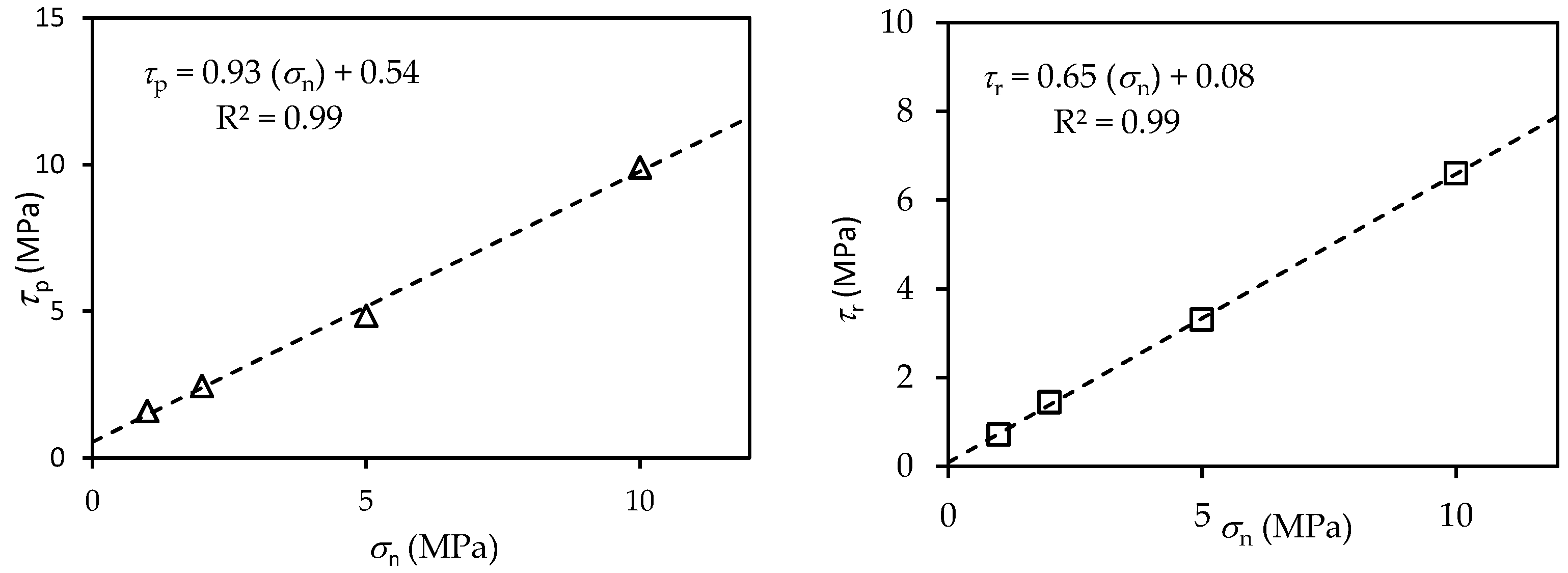
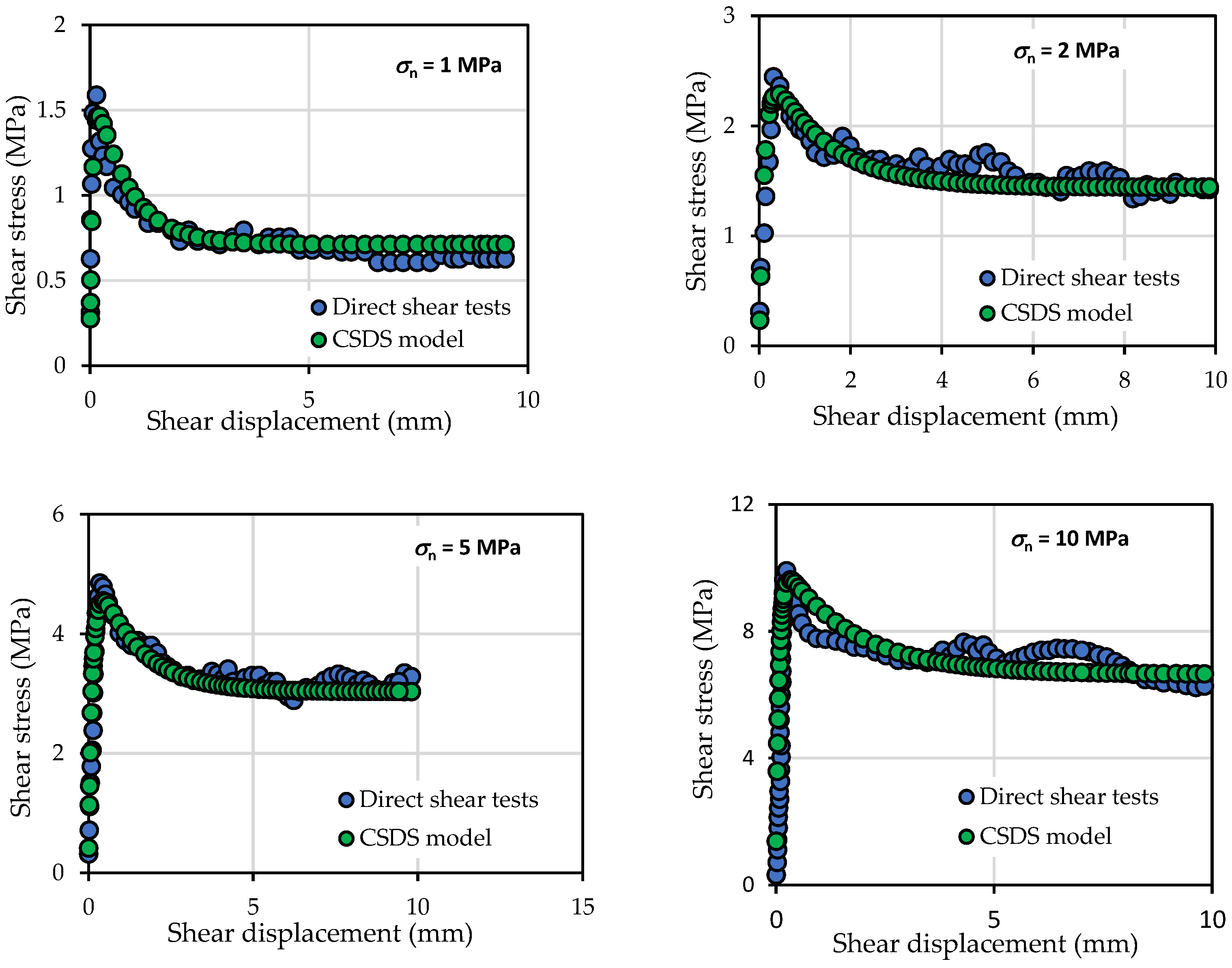
3. Experimental Setting

The application of the CSDS to represent observable large-scale slope instability is showcased through a detailed case study geometrically analogous to conventional planar failure. This case study involves an active planar slide along the Ruinon rock slope (Valfurva, Central Alps, Italy), and it is selected because of the simplicity of the slope geometry, detailed topographical monitoring collected between 1997 and 2002, and recorded precipitation in this period. These data are used to evaluate the evolving stress conditions in place and ascertain the stability conditions with respect to the long-term parameters. The case study is first developed empirically using physical relationships to derive all CSDS model parameters. The stress conditions are derived from conventional planar failure geometry outlined previously while taking into consideration yearly rainfall. The case study is then re-evaluated using the available direct analog shear test results on granite presented below. The later approach offers a comprehensive framework toward explicitly describing the evolving shear stress conditions during an active rockslide using an experimental calibration. The experimental settings and topographical measurements for the study period were taken from [5].

The slope section of the Ruinon is located northeast of the municipality of Valfurva, Italy, and to the west of the tributary of the Adda River in the Upper Valtellina. The studied zone spans an elevation from 1700 to 2200 m above sea level. The rock slopes are characterized by the pre-Permian metamorphic rock of the Austroalpine Campo Nappe. The rock mass is composed of folded marbles and metabasites cut by four regional alpine fractures controlling the geometry of the instabilities [32,33]. The marbles are made of coarse-grained saccharoidal calcite or of calc-silicate with calcite, chlorite, and white micas [32]. Crosta and Agliardi [5] reported an extensive rockslide accumulation at the toe of the slope, emphasizing the active nature of this overall instability [5].

Table 2. Mechanical properties of rock mass (taken from [5]).

$\mathit{\mu }$ (kN/m3)	${\mathit{C}}_0$ (MPa)	${\mathit{T}}_0$ (MPa)	JRC	JCS (MPa)	${\mathit{\phi }}_{\mathbf{p}}$ (°)	${\mathit{\phi }}_{\mathbf{r}}$ (°)
26.7	73	12	9–14	11.8–28.4	26	24.5

presents the geomechanical properties of the rock mass presented by [5]. Figure 3 presents a cross-sectional diagram of the slope geometry considered in this study. Since 1960, the Ruinon slope has been involved in repeated instability due to heavy rainfall in 1960, 1983, 1987, and 1997 [5]. The instabilities could be seen by debris flows, rockfalls, and the progressive development of scarps and fractures with differential movements along the middle slope sector. That is the reason why the movement started accelerating and showing seasonal changes in displacement rates since 1997 (see Figure 4). In addition, the distribution of scarps and trenches suggests a possible slope expansion up to 2200 m (see Figure 3) involving more than 20 Mm³ of rock.

Three joint sets were identified along the corresponding failure zones highlighted in the figure. All three joint families strike near parallel to the rock slope and dip at an angle ranging from 48 to 70 degrees [10,34].

Table 3. Geometry of the rockslide at different zones and calculated normal loading.

Rockslide Zones	$\mathit{H}$ (m)	$\mathit{Z}$ (m)	$\mathit{b}$(m)	$\mathit{A}$ (m2)	ψp (°)	ψf (°)	$\mathit{W}$ (kN/m)
Zone I	125	140	99	70	34	64	274.3
Zone II	126	124	111	139	30	62	340.6
Zone III	124	123	127	219	21	41	415.2

Note: The definition of all symbols is given in Section 2.3.

lists the geometrical features of the three distinct failure zones identified in Figure 3, following the nomenclature for a planar failure analysis. $\mu$ is the unit weight (kN/${\mathrm{m}}^3$), and $T_0$ (MPa) is the tensile strength.

The topographical monitoring of the active landslides compiled from 1997 to 2002 as well as the recorded rainfall are presented in Figure 4 (taken from [5]). The plot shows three distinct monitoring points referred to as markers D5–12, D7, and D26. These markers correspond to the zones I, II, and III, respectively. Cumulative rainfall is also included in the plot for reference. A notable increase in the deformation was noted by [5] beyond 1998. This increase is significant along zone I, but it is also present along the other zones. The cumulative annual rainfall was used to estimate the water column elevation $Z_w$ as a function of the fracture system $Z$. Peak rainfall during the monitoring timeline (late 1998) corresponds in this analysis to $Z_w=Z$, and the balance is estimated at a proportional relation of this peak rain data point. Cumulative 12-months rain measurements and corresponding forces are tabulated in

Table 4. Estimated water column, corresponding forces following the planar failure framework, and derived effective normal stress acting on the sliding plane for the three failure zones.

Zone No.	Date	Rainfall (mm)	${\mathit{Z}}_{\mathit{w}}$ (m)	$\mathit{U}$ (kN/m)	$\mathit{v}$ (kN/m)	${\mathit{\sigma }\prime }_{\mathit{n}}$ (MPa)
Zone I	19 Jun. 1997	89.3	15.6	5484.8	1221.4	3.11
	24 Feb. 1998	261.2	46.3	16,092.9	10,514.8	2.89
	01 Nov. 1998	790.4	140.2	48,730.7	96,412.9	1.75
	09 Jul. 1999	698.5	123.9	43,065.2	75,297.7	1.99
	15 Mar. 2000	685.0	121.5	42,234.4	72,420.8	2.03
	20 Nov. 2000	765.1	135.7	47,166.6	90,323.1	1.82
	28. Jul. 2001	NA	-----	-----	------	-----
Zone II	19 Jun. 1997	89.3	14.05	9592.14	968.26	2.03
	24 Feb. 1998	261.2	41.24	28,148.32	8338.07	1.87
	01 Nov. 1998	790.4	124.8	85,202.8	76,395.6	1.22
	09 Jul. 1999	698.5	110.3	75,303.4	59,674.7	1.35
	15 Mar. 2000	685.0	108.2	73,842.4	57,381.6	1.37
	20 Nov. 2000	765.1	120.1	81,980.4	70,726.2	1.26
	28. Jul. 2001	NA	-----	-----	------	-----
Zone III	19 Jun. 1997	89.3	13.9	14,889.8	940.9	1.69
	24 Feb. 1998	261.2	40.6	43,960.9	8101.1	1.55
	01 Nov. 1998	790.4	123.0	132,234	74,207.7	1.04
	09 Jul. 1999	698.5	108.7	116,849.7	57,945.3	1.14
	15 Mar. 2000	685.0	106.6	114,602.8	55,738.3	1.15
	20 Nov. 2000	765.1	119.1	128,009	69,541.5	1.06
	28. Jul. 2001	NA	-----	-----	------	-----

. It should be noted that the water column from one date to another only represents the water added due to the rainfall that occurred in that period. Monitoring data for the water left the system were not available for the calculations. This limitation is further discussed in Section 6. The table also lists the corresponding effective normal stresses ${\sigma \prime }_n$ acting on the failure planes for the three failure zones. The selected approach for the water column estimation is deemed reasonable as they correspond well to the observed changes in the deformation rates and field observations reported by [5]. The impact of this assumption is summarily assessed in Section 5.

The next two sections present the proposed approach to integrate the proven formulations and CSDS formulations presented in Section 2 toward describing the full shear stress–displacement curve. First, the acknowledged empirical principles are implemented to describe the relevant mechanical properties with respect to the effective normal stress conditions for different dates along the three zones. Then, experimental lab data of very similar rock samples are used to explicitly calibrate the model.

4. Empirical Integration Method

The evolving stress conditions of active rockslides are represented using the CSDS model calibrated with empirical relationships presented previously. The peak and residual shear stress ${\tau }_p$ and ${\tau }_r$ are derived from the Barton criteria (Equation (7)) using parameters listed in Table 2. The peak displacement $u_p$ is derived using the calibrated version of Equation (8) for tested granite presented in Section 3, which is discussed in Section 6, and the effective normal stress evaluated for the different loading zones listed in Table 4. The shear displacement at residual state $u_r$ is evaluated from the corresponding mobilized JRC from Figure 1, where $i$ is determined using Equation (10), which is approximately equal to 10 times $u_p$. The parameters $a$ through $e$ are then derived using Equations (2)–(6).

The physical properties estimated using empirical relationships and the corresponding CSDS parameters obtained using Equations (2)–(6) are presented in

Table A1. Physical parameters of the rockslides derived from empirical relationships (Equations (7)–(11)) and corresponding CSDS parameters (Equations (2)–(6)).

Zone No.	Date	${\mathit{\sigma }}_{\mathit{n}}$ (MPa)	${\mathit{\tau }}_{\mathit{p}}$ (MPa)	${\mathit{u}}_{\mathit{p}}$ (mm)	${\mathit{\tau }}_{\mathit{r}}$ (MPa)	${\mathit{u}}_{\mathit{r}}$ (mm)	a	b	c	d	e
Zone I	19-06-97	3.11	1.52	0.478	1.42	4.78	1.42	0.16	1.05	1.58	8.23
	24-02-98	2.89	1.41	0.475	1.32	4.75	1.32	2.23	1.05	3.54	4.49
	01-11-98	1.75	0.85	0.453	0.80	4.53	0.80	1.65	1.10	2.45	4.50
	09-07-99	1.99	0.97	0.459	0.91	4.59	0.91	1.78	1.09	2.68	4.50
	15-03-00	2.03	0.99	0.460	0.92	4.60	0.92	1.79	1.09	2.72	4.50
	20-11-00	1.82	0.89	0.455	0.83	4.55	0.83	1.68	1.10	2.51	4.50
Zone II	19-06-97	2.03	0.99	0.459	0.93	4.60	0.93	0.11	1.01	1.03	8.52
	24-02-98	1.87	0.91	0.456	0.85	4.56	0.85	0.10	1.10	0.95	8.50
	01-11-98	1.22	0.60	0.438	0.55	4.38	0.55	0.06	1.14	0.62	8.89
	09-07-99	1.35	0.66	0.442	0.61	4.42	0.61	0.07	1.13	0.69	8.82
	15-03-00	1.37	0.67	0.443	0.62	4.43	0.62	0.07	1.13	0.69	8.81
	20-11-00	1.26	0.61	0.439	0.57	4.39	0.57	0.07	1.14	0.64	8.87
Zone III	19-06-97	1.69	0.83	0.452	0.77	4.52	0.77	0.09	1.11	0.86	8.66
	24-02-98	1.55	0.76	0.448	0.71	4.48	0.71	0.09	1.12	0.79	8.72
	01-11-98	1.04	0.51	0.432	0.47	4.32	0.47	0.05	1.16	0.53	9.01
	09-07-99	1.14	0.55	0.435	0.52	4.35	0.52	0.06	1.15	0.58	8.95
	15-03-00	1.15	0.56	0.436	0.52	4.36	0.52	0.06	1.15	0.58	8.94
	20-11-00	1.06	0.52	0.433	0.52	4.33	0.49	0.06	1.16	0.54	8.99

in Appendix A.

Table 5. Computed shear stress (Equation (1)) and evolving long-term stress ratio (Equation (11)) using CSDS parameters from Table A1 and Equation (1).

Zone No.	Date	${\mathit{\sigma }}_{\mathit{n}}$(MPa)	Displacement (mm)	Shear Stress (MPa)	JRCc-m	$\mathit{\xi }$	${\mathit{\tau }}_{\mathit{L}}$(MPa)
Zone I	19 Jun. 1997	3.11	18.135	1.42	0.78	0.97	1.43
	24 Feb. 1998	2.89	60.449	1.32	0.76	0.97	1.34
	01 Nov. 1998	1.75	598.45	0.80	0.62	0.97	0.82
	09 Jul. 1999	1.99	822.11	0.91	0.65	0.97	0.93
	15 Mar. 2000	2.03	1426.6	0.92	0.65	0.97	0.95
	20 Nov. 2000	1.82	2133.9	0.83	0.63	0.97	0.85
Zone II	28. Jul. 2001	2.03	12.007	0.93	0.65	0.97	0.96
	19 Jun. 1997	1.87	66.038	0.85	0.63	0.97	0.88
	24 Feb. 1998	1.22	342.19	0.55	0.60	0.97	0.57
	01 Nov. 1998	1.35	468.27	0.62	0.60	0.97	0.64
	09 Jul. 1999	1.37	744.42	0.62	0.57	0.97	0.65
	15 Mar. 2000	1.26	1224.7	0.58	0.55	0.97	0.60
Zone III	20 Nov. 2000	1.69	5.0000	0.78	0.61	0.97	0.85
	28. Jul. 2001	1.55	10.000	0.71	0.59	0.97	0.76
	19 Jun. 1997	1.04	52.030	0.50	0.52	0.97	0.57
	24 Feb. 1998	1.14	95.050	0.52	0.54	0.97	0.55
	01 Nov. 1998	1.15	198.11	0.52	0.54	0.97	0.54
	09 Jul. 1999	1.06	372.21	0.49	0.53	0.97	0.53

computes the evolving stress conditions along the failure plane considered based on the computed model parameters presented in Table A1 and using Equation (1). The table also presents the long-term shear strength ratios and the corresponding long-term shear strength evaluated using Equation (11). Figure 5 plots the evolving shear stress conditions along the failure surface.

The global trends from Figure 5 for all three zones display an overall decrease in shear stress along with the failure plan. The largest and smallest shear stresses sustained during the period are along the rockslides in zones I and III, which match the cumulative displacement. The figure also highlights that the shear stress was at its maximum in zone I in late 1997 and mid-1998, which corresponded well with the time of the rockslide reported by [5]. The sudden decrease in shear stress toward the end of 1998 may be attributed to the elevated water pressure along with the joint failure, as indicated in Table 4. These conditions expedited the displacement rate, particularly along zone I beyond 1998, which is clearly evidenced by the monitored data presented in Figure 4. As is also shown in Figure 5, except for zone I, there is no risk of failure due to acceleration of displacement in the other zones.

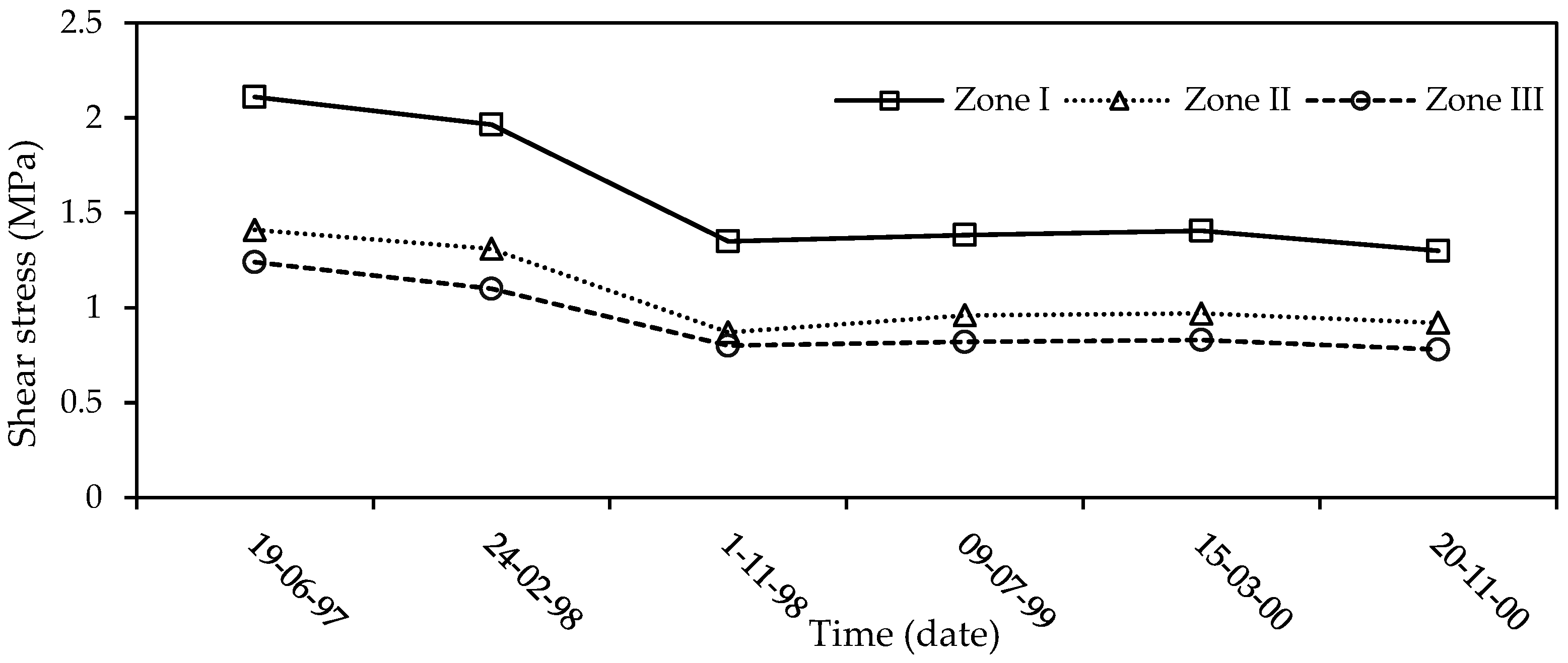
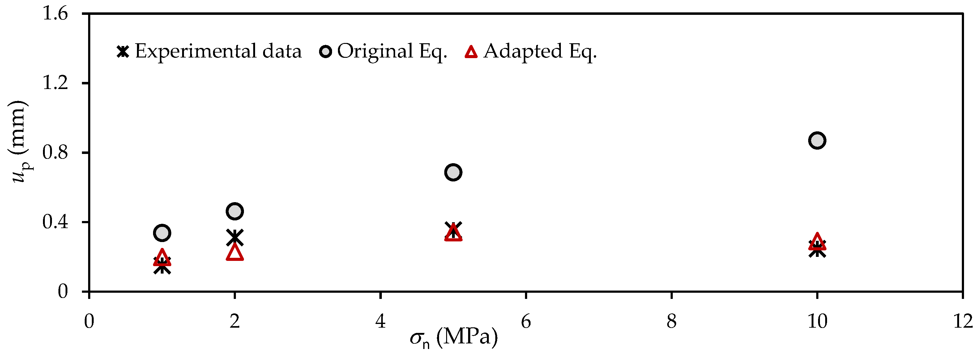
5. Experimental Calibration Approach

5.1. Experimental Analog

Direct shear tests reported by [35] for representative material (e.g., natural (unmated) granite fracture samples taken from the Flivik quarry outside Oskarshamn in Sweden) were selected in this section to explicitly calibrate the CSDS model. The data sets serve as a physical analog in subsequent analyses to exemplify the experimental application of CSDS and represent the stress condition of a rockslide event.

Zou and Cvetkovic [35] used the data from samples of 70 mm by 100 mm that were tested by [36] using a direct shear machine, which were manufactured at the Research Institutes of Sweden. The samples were tested under CNL conditions under normal stress values ${\sigma }_n$ of 1, 2, 5, and 10 MPa.

Table 6. Mechanical properties of granitic samples tested under direct shear (taken from [35]). $S_0$ is the uniaxial compressive strength of the intact rock.

Young’s Modulus (GPa)	${\mathit{s}}_0$ (MPa)	${\mathit{\phi }}_{\mathit{b}}$ (°)
73	255	22.2

summarizes the relevant geomechanical properties of the intact rock. Figure 6 plots the peak and residual shear strength of the tested samples with respect to normal stress during the direct shear tests. The linear regression is best fitted in the plots to provide a pragmatic relationship for ${\tau }_p-{\sigma }_n$ and ${\tau }_p-{\sigma }_n$ in subsequent analyses (Equations (18) and (19)). The physical measurements obtained from the direct shear tests and the corresponding model parameters $a$ through $e$ computed using Equations (2)–(6) are presented in Appendix A (see

Table A2. Shear parameters measured from direct shear tests on granitic samples, presented in [33], and corresponding CSDS parameters computed using (Equations (2)–(6)).

${\mathit{\sigma }}_{\mathit{n}}$ (MPa)	${\mathit{\tau }}_{\mathit{p}}$ (MPa)	${\mathit{u}}_{\mathit{p}}$ (mm)	${\mathit{\tau }}_{\mathit{r}}$ (MPa)	${\mathit{u}}_{\mathit{r}}$ (mm)	$\mathit{a}$	$\mathit{b}$	$\mathit{c}$	$\mathit{d}$	$\mathit{e}$
1	1.59	0.15	0.71	3.87	0.71	1.07	1.3	1.78	16.56
2	2.44	0.31	1.44	6.28	1.44	1.28	0.79	2.83	8.69
5	4.85	0.35	3.03	6.41	3.03	2.40	0.78	5.43	7.71
10	9.9	0.25	6.64	8.2	6.64	3.79	0.61	10.43	13.37

). Equation (1) was then used to plot the shear stress with respect to displacement in Figure 7 using the parameters listed in Table A2. The corresponding stress–displacement data measured during the direct shear tests are also plotted in the figure. These plots indicate a very suitable correspondence between the CSDS calibration and the laboratory measurements during the direct shear tests. The long-term shear strength ratios achieved during the tests were also computed using Equation (11). The long-term parameters are presented in

Table 7. Long-term parameters for the granite tested under direct shear tests derived using Equation (11).

${\mathit{\sigma }}_{\mathit{n}}$ (MPa)	JRCc-m	$\mathit{\xi }$	${\mathit{\tau }}_{\mathit{L}}$ (MPa)
1	8.87	0.64	1.02
2	8.12	0.69	1.70
5	6.0	0.76	3.66
10	5.6	0.75	7.43

.

$${\tau }_p=0.93\left({\sigma }_n\right)+0.54$$

(18)

$${\tau }_r=0.65\left({\sigma }_n\right)+0.08$$

(19)

5.2. Applied Calibration

The evolving stress conditions of active rockslides during the monitoring period are represented using the laboratory experimental behavior of granitic samples under direct shear tests, as presented in Section 3. The relevant physical parameters are listed in Table 6 and Table 7 and Table A2 in Appendix A. The experimentally calibrated parameters are transposed to the studied rockslides to derive the CSDS parameters at different times. These parameters are listed in

Table A3. Physical parameters derived from experimental measurements and relevant relationships and CSDS parameters computed using (Equations (2)–(6)).

Zone No.	Date	${\mathit{\sigma }}_{\mathit{n}}$ (MPa)	${\mathit{\tau }}_{\mathit{p}}$ (MPa)	${\mathit{u}}_{\mathit{p}}$ (mm)	${\mathit{\tau }}_{\mathit{r}}$ (MPa)	${\mathit{u}}_{\mathit{r}}$	a	b	c	d	e
Zone I	19-06-97	3.11	3.4	0.44	2.10	8.8	2.11	1.67	0.57	3.78	6.58
	24-02-98	2.89	3.2	0.44	1.96	8.7	1.96	1.58	0.57	3.54	6.61
	1-11-98	1.75	2.15	0.41	1.22	8.1	1.22	1.22	0.62	2.45	6.74
	09-07-99	1.99	2.38	0.41	1.38	8.3	1.38	1.30	0.60	2.68	6.70
	15-03-00	2.03	2.41	0.42	1.40	8.3	1.41	1.31	0.60	2.72	6.69
	20-11-00	1.82	2.22	0.41	1.27	8.2	1.27	1.25	0.61	2.51	6.73
Zone II	19-06-97	2.03	2.41	0.42	1.41	8.3	1.41	1.29	0.60	2.70	6.71
	24-02-98	1.87	2.27	0.41	1.31	8.2	1.31	1.24	0.61	2.54	6.74
	1-11-98	1.22	1.66	0.38	0.88	7.6	0.88	1.00	0.65	1.90	6.92
	09-07-99	1.35	1.79	0.39	0.96	7.8	0.96	1.06	0.64	2.02	6.87
	15-03-00	1.37	1.80	0.39	0.97	7.8	0.97	1.06	0.64	2.04	6.87
	20-11-00	1.26	1.70	0.38	0.91	7.7	0.91	1.02	0.65	1.93	6.90
Zone III	19-06-97	1.69	2.10	0.40	1.20	8.1	1.19	1.18	0.62	2.37	6.80
	24-02-98	1.55	1.97	0.40	1.10	8.0	1.10	1.13	0.63	2.22	6.80
	1-11-98	1.04	1.50	0.37	0.80	7.4	0.80	0.95	0.67	1.71	7.00
	09-07-99	1.14	1.59	0.38	0.82	7.5	0.80	0.98	0.66	1.81	6.90
	15-03-00	1.15	1.60	0.38	0.83	7.6	0.83	0.98	0.66	1.82	6.95
	20-11-00	1.06	1.52	0.37	0.78	7.5	0.78	0.96	0.67	1.74	6.90

of Appendix A. The evolving shear stress is then computed using Equation (1). The explicit computation results and corresponding long-term shear strength are presented in

Table 8. Shear stress derived by the CSDS model (Equation (1)) and parameters from Table A3 (see Appendix A).

Zone No.	Date	${\mathit{\sigma }}_{\mathit{n}}$ (MPa)	Displacement (mm)	Shear Stress (MPa)	JRCc-m	$\mathit{\xi }$	${\mathit{\tau }}_{\mathit{L}}$ (MPa)
Zone I	19-06-97	3.11	18.135	2.11	14.5	0.71	2.2
	24-02-98	2.89	60.449	1.96	14.2	0.71	1.85
	01-11-98	1.75	598.45	1.40	13.1	0.69	1.38
	09-07-99	1.99	822.11	1.38	13.3	0.69	1.65
	15-03-00	2.03	1426.6	1.41	13.3	0.69	1.67
	20-11-00	1.82	2133.9	1.30	13.1	0.69	1.53
Zone II	19-06-97	2.03	12.007	1.41	13.3	0.69	1.68
	24-02-98	1.87	66.038	1.31	13.2	0.69	1.57
	01-11-98	1.22	342.19	0.87	12.8	0.67	1.12
	09-07-99	1.35	468.27	0.96	12.9	0.68	1.21
	15-03-00	1.37	744.42	0.97	12.9	0.68	1.22
	20-11-00	1.26	1224.7	0.92	12.9	0.67	1.15
Zone III	19-06-97	1.69	5.0000	1.24	13.0	0.69	1.45
	24-02-98	1.55	10.000	1.01	13.0	0.68	1.35
	01-11-98	1.04	52.030	0.80	12.8	0.67	1.00
	09-07-99	1.14	95.050	0.82	12.8	0.67	1.06
	15-03-00	1.15	198.11	0.83	12.8	0.67	1.07
	20-11-00	1.06	372.21	0.80	12.8	0.67	1.02

. The evolving shear stress values for the different zones are also plotted in Figure 8.

The results plotted in Figure 8 present apparently similar general trends with respect to results obtained from empirical estimates. It is, however, noticed that the shear stress obtained by the empirical evaluations (see Figure 5) is notably less than those shown in Figure 8. The underestimation of the shear stress may be related to imposing empirical limitations. These variations are to be expected considering the experimental analog selected for this part of the analysis. The shear stress obtained by the experimental analog better represents progressive shear stress along the active rockslides with respect to the monitored displacement rate and long-term shear strength. The estimated shear stress for zone I presents larger values compared to those estimated for zones II and III, which correspond well with the accelerated displacement rate in zone I in comparison with the two other zones. In addition, the shear stress is at its maximum along the rockslide in zone I in late 1997 and mid-1998, which corresponds well with the data presented in Table 8, in which only the maximum shear stress in zone I obtained in those dates exceeds the long-term shear strength of the rock mass derived from the experimental measurements. This observation represents well the field observations reported by [5], in which the ancient rockslides in zone III caused instability along zone I, particularly during the rainfall in previous years. The relationship between shear stress with respect to shear strength for the three zones corresponds well with the atmospheric and topographical phenomena observed during the study period.

6. Discussion

This study presented a robust framework to represent evolving stress conditions for active rockslides through the implementation of the CSDS model and calibration from either empirical notions or experimental laboratory conditions. The findings emphasize that the experimental analog implemented in this work and the field data collection could partly represent the true behavior observed from the case study. However, this approach would be ideal but not always practical due to field limitations. Hence, the empirical approach is an interesting alternative to estimate the in-situ conditions and apply the proposed conceptual framework. In fact, the dual approach of empirical and experimental corroboration of the complete stress profiles from topographical monitoring offers a meaningful solution with built-in redundancy. This proof of concept paves the way for a true empirical experimental calibration of stress–strain behavior for active rockslides.

In this study, the shear displacement at peak was determined using Equation (8). The equation had been previously validated by [28] through an analysis of the experimental data. It is proposed that this relationship can be further improved by site-specific calibration based on the laboratory evidence of available data sets. The equation is, therefore, rewritten by replacing the empirical parameters with the variables to be calibrated as follows:

$$u_p=\mathrm{a}.L^{\mathrm{b}}{\left({\displaystyle \frac{{\sigma }_n}{JCS }}\right)}^{\mathrm{c}}\cos \left(JRC\mathit{log}\left[{\displaystyle \frac{JCS}{{\sigma }_n}}\right]\right)$$

(20)

The relationship is revisited through experimental calibration using the mechanical properties and experimental data obtained from direct shear tests conducted on granite with different roughness, as outlined in Table 6 and Table A2 of Appendix A. Following the application of a solver tool, parameters a, b, and c for Equation (20) are determined as follows: $a=0.000452$, $b=0.041$, and $c=0.093$.

Figure 9 illustrates comparisons between the $u_p$ obtained from experimental tests and those derived from Equations (8) and (19). It is evident that the $u_p$ values obtained from the calibrated equation, particularly for each normal loading applied to granite samples with specific roughness, closely align with the experimental data, while the $u_p$ values calculated using the original equation (Equation (8)) tend to overestimate the results. Consequently, the calibrated equation specific to the tested granite was used in the analysis of the case study to ensure accurate $u_p$ values are obtained.

The available studies have shown that there is a scale effect on the rock surface roughness, which seems to be responsible for the scale effect on the shear behavior of rock joints in the laboratory scale [15,16,37,38,39,40]. Nonetheless, recently proposed models provided constitutive models for an upscaling analysis of the mechanical properties and shear behavior in large-scale fractured rock masses through the calculation of evolving shear stress [19,20,21,22]. When there is not enough monitoring data, the test data obtained in the laboratory must be used for the validation of the proposed constitutive model, which again involves the scale effect.

Of relevance to future work, the present study transposed laboratory measurements explicitly to the field without additional considerations given to the scale effect. However, in the absence of a universally acknowledged scaling relationship or the means to explicitly validate such an assumption, the consistent re-evaluation of the long-term shear strength ratio with respect to mobilized JRC offers a robust alternative to quantify rock slope progression toward a long-term response. Topographical monitoring and associated changes in displacement trends remain a robust avenue to validate the experimental and empirical assumptions when the physical model is well understood. The approach may also be transposed to more complex geometries with multiple intersecting surfaces (i.e., wedges). Such applications would be better approached through numerical implementation in a discrete element model code (a similar application was trialed for the analysis of mine-induced seismicity by [23] with a boundary element model code).

In this study, the experimental data of a natural rock (e.g., granite) were used for the experimental calibration of the proposed approach. The experimentally calibrated parameters are transposed to the studied rockslides to derive the CSDS parameters at different times. The properties of the tested rock were different from the rockslide. Nevertheless, the application of the proposed conceptual framework remains valid and could be further enhanced with site-specific properties.

It is further noted that the CSDS formulation, in its present explicit form, does not provide the means to account for variable displacement rates. In extensive laboratory trials on direct shear tests of rock interfaces, Wang et al. [41] failed to report the meaningful influence of displacement during conventional direct shear tests. It is more plausible that the influence of strain rate is negligible for the achievable range of conventional direct shear tests. Such a simplification is further warranted considering the intended application of the proposed framework. Applying CSDS to very rapid rockslides (i.e., near failure) serves no practical engineering purpose beyond back analyses (where the influence of very rapid strain would need to be considered).

The application of CSDS to represent large-scale rockslides is more suitable for prevention applications, where active stress conditions are consistently monitored and re-evaluated in the early stages of instability. The long-term shear strength ratio offers a very pragmatic perspective on long-term behavior, which is readily compared with current stress conditions derived from CSDS representations to show the stability of the rockslide. It should be noted that the purpose of the proposed conceptual approach in this study is to offer guidance and a quantifiable perspective toward global stability. However, there are certain limitations with data acquisition and geometrical simplifications, which hinder accurate site-specific statements toward stability. The proposed approach could be further leveraged by integrating risk evaluation and mitigation analysis. The quantifiable shear stress acting on the failure plane can be compared with long-term shear strength and re-evaluated by parametrically changing certain parameters to investigate the impact of certain external factors on the stability conditions (e.g., excessive rain, seismic event, erosion of the toe of the slope).

The present work established a relationship between the evolving stress conditions and the measured displacement. Accordingly, predictions and stability assessments derived from punctual investigation at specific time intervals, such as the analyses presented above, reflect limit state conditions without adjustment (i.e., Factor of Safety (FoS) = 1). It is asserted that the limit state factors, reflective of the confidence in the input parameters, could be applied following a conventional geotechnical stability analysis precept (see, for example, [42]). A limit state condition analysis could, therefore, be combined with the conceptual framework presented in this study to evaluate the investigated conditions and establish associated FoS.

The presented results suggest a notable influence of groundwater conditions on the active loading profile of the slope. Assuming limited changes in the overall geometry of the system, normal stress acting on the failure surfaces dictates normal stresses and, therefore, directly influences most parameters. It could be argued that high alpine rock slopes with a non-negligible uphill footprint and annual precipitations of approximately 0.7 m would have vertical joints nearly saturated for a good portion of the year. Depending on the rock mass porosity, the water head could potentially even exceed the vertical scarp span. Such assumptions would lead to two fundamental changes in computational results as follows: higher effective shear loading along the failure plane and lower long-term shear–strength ratio. Both aspects would theoretically offer a more conservative consideration toward any stability analysis. It emphasized, however, that a more robust application of this framework should include water head monitoring along the slopes.

7. Conclusions

This work aimed to contribute to the realization of a critical movement of a sliding plane by describing the progressive shear stress of rockslides. To achieve this purpose, the incorporation of several proven models into the updated version of the CSDS model [26] was proposed. Through the suggested method, the plane failure analysis is used to determine the normal load (or field load) acting on the joints. The updated CSDS model, along with the Barton shear strength, was then used to calculate CSDS model parameters through empirical and experimental evaluations. The proposed chain function of the integrated model can describe a progressive shear stress curve of a rockslide with the use of a monitored displacement in the field. Comparisons of the long-term shear strength of a joint and the progressive shear stress lead to the realization of a probable critical state (or failure) of a sliding plane. This study contributed to a comprehensive framework that integrates in situ topographical monitoring with experimental and empirical geomechanical data to develop a representative model capturing the evolving stress conditions during a rockslide event. The results first show the practical approach of the proposed framework for a simple rockslide. The results then suggest that both experimental and empirical calibration can yield applicable results. It is further surmised that applying both can enhance result reliability through redundancy.

References

1. Donati, D.; Stead, D.; Borgatti, L. The Importance of Rock Mass Damage in the Kinematics of Landslides. Geosciences 2023, 13, 52. [Google Scholar] [CrossRef]
2. Deng, D.; Simon, R.; Aubertin, M. Modelling shear and normal behaviour of filled rock joints. In GeoCongress 2006: Geotechnical Engineering in the Information Technology Age; ASCE: Reston, VA, USA, 2006; pp. 1–6. [Google Scholar]
3. Wyllie, D.C.; Mah, C. Rock Slope Engineering: Civil End Mining; CRC Press: London, UK, 2004. [Google Scholar]
4. Fukuzono, T. A new method for predicting the failure time of a slope. In Proceedings of the 4th International Conference and Field Workshop on Landslide, Tokyo, Japan, 23ߝ31 August 1985; pp. 145–150. [Google Scholar]
5. Crosta, G.B.; Agliardi, F. Failure forecast for large rock slides by surface displacement measurements. Can. Geotech. J. 2003, 40, 176–191. [Google Scholar]
6. Rose, N.D.; Hungr, O. Forecasting potential rock slope failure in open pit mines using the inverse-velocity method. Int. J. Rock Mech. Min. Sci. 2007, 44, 308–320. [Google Scholar] [CrossRef]
7. Kodama, J.; Nishiyama, E.; Kaneko, K. Measurement and interpretation of long-term deformation of a rock slope at the Ikura limestone quarry, Japan. Int. J. Rock Mech. Min. Sci. 2009, 46, 148–158. [Google Scholar] [CrossRef]
8. Oppikofer, T.; Jaboyedoff, M.; Blikra, L.; Derron, M.H.; Metzger, R. Characterization and monitoring of the Åknes rockslide using terrestrial laser scanning. Nat. Hazards Earth Syst. Sci. 2009, 9, 1003–1019. [Google Scholar]
9. Basahel, H.; Mitri, H. Application of rock mass classification systems to rock slope stability assessment: A case study. J. Rock Mech. Geotech. Eng. 2017, 9, 993–1009. [Google Scholar]
10. Storni, E.; Hugentobler, M.; Manconi, A.; Loew, S. Monitoring and analysis of active rockslide-glacier interactions (Moosfluh, Switzerland). Geomorphology 2020, 371, 107414. [Google Scholar] [CrossRef]
11. Vibert, C.; Arnould, M.; Cojean, R.; Le Cleach, J.M. Essai de prévision de rupture d’un versant montagneux à Saint-Etienne-de-Tinée. In Proceedings of the Fifth International Symposium on Landslides, Lausanne, Switzerland, 10ߝ15 July 1988; pp. 789–792. [Google Scholar]
12. Sharon, R.; Rose, N.; Rantapaa, M. Design and development of the Northeast layback of the Betze-post open pit. In Proceeding of the SME Annual Meeting, Salt Lake City, UT, USA, 28 February–2 March 2005; pp. 05–09. [Google Scholar]
13. Patton, F.D. Multiple Modes of Shear Failure in Rock and Related Materials. Ph.D. Thesis, University of Illinois at Urbana-Champaign, Champaign, IL, USA, 1966. [Google Scholar]
14. Ladanyi, B.; Archambault, G. Simulation of shear behavior of a jointed rock mass. In Proceedings of the 11th US Symposium on Rock Mechanics (USRMS), Berkeley, CA, USA, 16–19 June 1969. OnePetro. [Google Scholar]
15. Barton, N.; Choubey, V. The shear strength of rock joints in theory and practice. Rock Mech. 1977, 10, 1–54. [Google Scholar]
16. Bandis, S.; Lumsden, A.C.; Barton, N.R. Experimental studies of scale effects on the shear behaviour of rock joints. Int. J. Rock Mech. Min. Sci. Geomech. Abstr. 1981, 18, 1–21. [Google Scholar]
17. Barton, N. Modelling Rock Joint Behavior from In Situ Block Tests: Implications for Nuclear Waste Repository Design; Office of Nuclear Waste Isolation, Battelle Project Management Division: Columbus, OH, USA, 1982; Volume 308. [Google Scholar]
18. Grasselli, G.; Egger, P. Constitutive law for the shear strength of rock joints based on three-dimensional surface parameters. Int. J. Rock Mech. Min. Sci. 2003, 40, 25–40. [Google Scholar]
19. Barton, N.; Bandis, S.; Bakhtar, K. Strength, deformation and conductivity coupling of rock joints. Int. J. Rock Mech. Min. Sci. Geomech. Abstr. 1985, 22, 121–140. [Google Scholar] [CrossRef]
20. Xie, S.; Lin, H.; Han, Z.; Duan, H.; Chen, Y.; Li, D. A New Shear Constitutive Model Characterized by the Pre-Peak Nonlinear Stage. Minerals 2022, 12, 1429. [Google Scholar] [CrossRef]
21. Lin, H.; Xie, S.; Yong, R.; Chen, Y.; Du, S. An empirical statistical constitutive relationship for rock joint shearing considering scale effect. Comptes Rendus. Mécanique 2019, 347, 561–575. [Google Scholar] [CrossRef]
22. Cheng, T.; Guo, B.H.; Sun, J.H.; Tian, S.X.; Sun, C.X.; Chen, Y. Establishment of constitutive relation of shear deformation for irregular joints in sandstone. Rock Soil Mech. 2022, 43, 4. [Google Scholar]
23. Simon, R. Analysis of Fault-Slip Mechanisms in Hard Rock Mining. Ph.D. Thesis, McGill University, Montreal, QC, Canada, 1999. [Google Scholar]
24. Simon, R.; Aubertin, M.; Deng, D. Estimation of post-peak behaviour of brittle rocks using a constitutive model for rock joints. In Proceedings of the 56th Canadian Geotechnical Conference, Winnipeg, MB, Canada, 29 September–1 October 2003. [Google Scholar]
25. Tremblay, D.; Simon, R.; Aubertin, M. A constitutive model to predict the hydromechanical behavior of rock joints. In Proceedings of the GeoOttawa, Ottawa, ON, Canada, 21–24 October 2007; pp. 2011–2018. [Google Scholar]
26. Deiminiat, A.; Aubertin, J.D.; Ethier, Y. On the calibration of a shear stress criterion for rock joints to represent the full stress-strain profile. J. Rock Mech. Geotech. Eng. 2024, 16, 379–392. [Google Scholar] [CrossRef]
27. Asadollahi, P. Stability Analysis of a Single Three-Dimensional Rock Block: Effect of Dilatancy and High-Velocity Water Jet Impact. Ph.D. Thesis, The University of Texas at Austin, Austin, TX, USA, 2009. [Google Scholar]
28. Asadollahi, P.; Tonon, F. Constitutive model for rock fractures: Revisiting Barton’s empirical model. Eng. Geol. 2010, 113, 11–32. [Google Scholar] [CrossRef]
29. Wang, M.; Cai, M. A simplified model for time-dependent deformation of rock joints. Rock Mech. Rock Eng. 2021, 54, 1779–1797. [Google Scholar] [CrossRef]
30. Wang, M. Modeling Time-Dependent Deformation Behavior of Jointed Rock Mass. Ph.D. Thesis, Laurentian University of Sudbury, Greater Sudbury, ON, Canada, 2022. [Google Scholar]
31. Hoek, E.; Bray, J.D. Rock Slope Engineering, 3rd ed.; Taylor and Francis Group: London, UK, 1981. [Google Scholar]
32. Agliardi, F.; Crosta, G.; Zanchi, A. Structural constraints on deep-seated slope deformation kinematics. Eng. Geol. 2001, 59, 83–102. [Google Scholar] [CrossRef]
33. Manconi, A.; Kourkouli, P.; Caduff, R.; Strozzi, T.; Loew, S. Monitoring surface deformation over a failing rock slope with the ESA sentinels: Insights from Moosfluh instability, Swiss Alps. Remote Sens. 2018, 10, 672. [Google Scholar] [CrossRef]
34. Glueer, F.; Loew, S.; Manconi, A. Paraglacial history and structure of the Moosfluh Landslide (1850–2016), Switzerland. Geomorphology 2020, 355, 106677. [Google Scholar] [CrossRef]
35. Zou, L.; Cvetkovic, V. A new approach for predicting direct shear tests on rock fractures. Int. J. Rock Mech. Min. Sci. 2023, 168, 105408. [Google Scholar]
36. Jacobsson, L.; Ivars, D.M.; Kasani, H.A.; Johansson, F.; Lam, T. Experimental program on mechanical properties of large rock fractures. IOP Conf. Ser. Earth Environ. Sci. 2021, 833, 012015. [Google Scholar] [CrossRef]
37. Fardin, N. Influence of structural non-stationarity of surface roughness on morphological characterization and mechanical deformation of rock joints. Rock Mech. Rock Eng. 2008, 41, 267–297. [Google Scholar]
38. Tan, R.; Chai, J.; Cao, C. Experimental investigation of the permeability measurement of radial flow through a single rough fracture under shearing action. Adv. Civ. Eng. 2019, 1, 6717295. [Google Scholar]
39. Deiminiat, A.; Li, L.; Zeng, F. Experimental study on the minimum required specimen width to maximum particle size ratio in direct shear tests. CivilEng 2022, 3, 66–84. [Google Scholar] [CrossRef]
40. Deiminiat, A.; Li, L.; Zeng, F.; Pabst, T.; Chiasson, P.; Chapuis, R. Determination of the Shear Strength of Rockfill from Small-Scale Laboratory Shear Tests: A Critical Review. Adv. Civ. Eng. 2020, 1, 8890237. [Google Scholar] [CrossRef]
41. Wang, G.; Zhang, X.; Jiang, Y.; Wu, X.; Wang, S. Rate-dependent mechanical behavior of rough rock joints. Int. J. Rock Mech. Min. Sci. 2016, 83, 231–240. [Google Scholar]
42. Holtz, R.D.; Kovacs, W.D.; Sheahan, T.C. An Introduction to Geotechnical Engineering, 3rd ed.; Pearson: New York, NY, USA, 2022. [Google Scholar]
Figure 1. Mobilized JRC developed by [28]; u m = mobilized displacement. The computed relationship assumes φ r = 30° and i = 15°.
Geosciences 15 00139 g001
Figure 2. Geometries of a plane slope: (a) tension crack in the upper slope; (b) tension crack in the face, after [31].
Geosciences 15 00139 g002
Figure 3. Geometry of the rockslide along the Ruinon rock face, after [5].
Geosciences 15 00139 g003
Figure 4. Monitored displacement pattern versus time at three different monitoring points close to the study zones, taken from [5].
Geosciences 15 00139 g004
Figure 5. Evolving shear stress along the failure zones derived from the empirically calibrated CSDS model using topographical monitoring of the Ruinon rockslides from 1997 to late 2000.
Geosciences 15 00139 g005
Figure 6. Linear regressions of peak and residual shear strength with respect to normal stress during direct shear tests on granitic samples. Experimental data taken from [35].
Geosciences 15 00139 g006
Figure 7. Composition of shear stress–shear displacement curves obtained by experimental shear tests and the CSDS model based on experimental results presented in [35].
Geosciences 15 00139 g007
Figure 8. Evolving shear stress for the three zones derived from the experimental calibration of CSDS.
Geosciences 15 00139 g008
Figure 9. Comparisons between the u p values obtained using experimental tests and those calculated by Equation (8) and calibrated Equation (8) for granite (Equation (18)) (data taken from [35]).
Geosciences 15 00139 g009