Abstract
The morphological characteristics of catchments are key controls on how flow is routed through catchments and the spatial and temporal dynamics of floods, therefore influencing the shape of hydrographs at any location. Here, we developed a hydro-morphic catchment classification to understand the extent to which various catchment characteristics act as controls on flood behaviour. The catchment characteristics include: size (as measured by gauge position in catchment and valley confinement at the gauge site), shape (elongation ratio and form factor), topography (catchment relief and longitudinal slope), and drainage network structure (drainage density). A total of 2452 high flow (near bankfull) and overbank flood hydrographs from rivers in 17 coastal catchments of New South Wales (NSW), Australia were used. Cluster analysis on hydrograph shape metrics of kurtosis, skewness, and rate-of-rise was performed to identify classes of hydrographs and their median shape. Three statistically distinct clusters were delineated for both high flows and overbank floods, and categorised as flashy, intermediate, and broad. Topographic characteristics of catchments (i.e., relief and longitudinal slope) were commonly among the dominant controls for all high flow and overbank flood hydrographs, excluding broad overbank floods. Drainage network structure (i.e., drainage density) also controlled flashy and intermediate high flows, and intermediate and broad overbank floods, while catchment size (i.e., gauge position in the network) influenced broad high flows. Catchment shape (i.e., elongation ratio) influenced broad overbank floods, and is a dominant control on flashy high flows, and intermediate and broad overbank floods. Overall, topographic controls were more useful for differentiating the hydrological behaviour of high flows relative to overbank floods. Understanding the relative control of different catchment morphometric characteristics on flow and flood behaviour can be used to identify the aspects of flood behaviour that are set by imposed controls and cannot therefore be realistically manipulated in management. A hydro-morphic classification can also be used in the design and calibration of hydrological models, tailoring their use to hydro-morphic catchment class.
1. Introduction
The hydrological characteristics of floods are controlled and governed by interactions between geological, climatic, and anthropogenic controls that operate at the catchment scale [1,2,3,4]. Early geomorphological research on the laws of drainage network composition and how they are influenced by relief, basin shape, tributary–trunk stream interactions, drainage pattern, and dissection set the foundations for analysing and understanding the internal dynamics of water flow through catchments, and by extension flood behaviour [4,5,6,7,8,9,10]. In more recent studies, various geological, climatic, hydrologic and land cover measures have been used to classify catchments [11,12,13,14]. To produce these classifications, geological measures, such as drainage area, slope, elevation, and topography, have been used [12,14,15,16]. In some studies, climatic and hydrological measures, such as the frequency and magnitude of flow, rainfall–runoff coefficients, and stream flow characteristics including rate-of-rise, time-to-peak, and catchment response time, have been used [11,17,18,19,20]. In other studies, the influence of anthropogenic disturbance on hydrological behaviour of catchments using measures such as land cover have been used [21,22,23].
Many studies indicated that flood dynamics, such as travel time, celerity, stage height, and rates of rise and fall, are all influenced by catchment morphometric characteristics, such as drainage area and shape, relief, and drainage density [4,5,8,9,10,24,25,26]. For example, catchments with steep slopes or high relief, high drainage density, and round shape are more likely to experience flash floods than catchments with gentler slopes, low relief, low drainage density, and elongated shape [27,28,29,30]. Other studies show that climatic (e.g., precipitation and storm properties) and geomorphic (e.g., soil properties) characteristics of catchments also play a role in flood generation and transfer processes [31,32,33,34]. For example, catchments with bare rocks soil and low infiltration may have a fast response compared to catchments where well-developed soils and permeability is high [35]. Catchments with considerable subsurface or near-surface flow contributions to streamflow may produce flow hydrographs that are flatter with a longer lag time from upstream to downstream [31]. Such conditions may control flood dynamics through the effect of soil moisture and water retention and storage on flood transmission behaviour [34]. Elsewhere, catchments that occur in moist mid-latitude climate zones may accumulate snowpacks that create annual melt and associated floods [33,34]. In some arid areas, a lack of precipitation and high evaporation may lead to dry soils with a high infiltration rate and a low flood generating potential [35]. In these catchments, geologic controls are less important than climatic or geomorphic controls on the hydrology of these catchments [17].
Given the complexities with which geologic, climatic, and geomorphic controls interact and influence flood behaviour, some previous studies have failed to find significant, measurable correlations between morphometric, climatic, and hydrologic characteristics of catchments [12,17,18,36]. However, from a management and flood mitigation perspective, it remains important to understand the extent to which catchment morphometric characteristics (called imposed controls) are deriving flood behaviour, and therefore cannot be manipulated, and separate these from other controls and influences (called flux controls) that can possibly be manipulated in-practice. Imposed controls are set by tectonic setting and lithology and do not readily adjust over geomorphic timeframes, whereas flux controls including water and sediment fluxes and interactions with vegetation can recurrently adjust over geomorphic timeframes [37].
One of the main limitations of catchment classification based on morphometric characteristics is that the measures are calculated at coarse scales, producing catchment-averaged data [38,39] that cannot account for the internal complexity and variability of these characteristics within a catchment [11,40]. Additionally, non-linear interactions between rainfall and runoff can have complex and unpredictable impacts on streamflow characteristics, making it difficult to accurately characterise the hydrological behaviour of a catchment [11,17,41,42].
A key method that serves to reduce variability and complexity is to cluster hydrographs based on their quantifiable shape characteristics and analyse the morphometrics of the catchments in which these hydrographs are produced [12,20,23]. This method (hereafter called hydro-morphic catchment classification) is a commonly used method of characterising and categorising catchments based on both hydrological and geomorphological features. This method requires extensive data collection and analysis before choosing or developing appropriate hydrological models [39,40]. Also, it can be used to help explain flood behaviour of catchments with similar morphometric and hydrologic characteristics, and to infer the possible hydrological behaviour of a new catchment with similar morphometric characteristics [12,41,43,44].
The appropriate selection of morphometrics is crucial for hydro-morphic classification. The best explanatory morphometrics (hereafter called dominant) are those that can be used to describe the shape, topography, size, and drainage network structure of a catchment, and are simple to measure [23,39,45]. As such, the most commonly used catchment morphometrics are elongation ratio (Er), form factor (Rf), catchment relief (Rh), drainage density (Dd), valley confinement at the gauge site (Vc), gauge position in the catchment (Gp), and average longitudinal slope upstream of the gauge site (Sl) (e.g., [12,17,21,30]).
Both Er and Rf describe the shape of a catchment. Er measures how elongate a catchment is, indicates the trunk stream–tributary configuration of a catchment, and can be used as a proxy for sub-catchment size and flow contributions along the trunk stream. Rf measures whether a catchment has a circular or elongate shape which influences the time-to-peak and flatness of the hydrograph peak. Rh and Sl represent catchment topography. Rh and Sl measure catchment average slope and channel bed slope, respectively, which affect hydrological responses to rainfall, infiltration rate, and stream flow celerity along the valley bottom.
Dd is a measure of drainage network structure. It is measured as the density of the stream network per unit area with a high drainage density indicating a dense network of streams. The Dd of the stream network in a catchment impacts surface flow generation, infiltration rate, and flow distribution [46]. Dd depends on various factors, such as topography, climate, vegetation cover, soil properties, and lithology [47,48]. The scale at which Dd is measured is important factor in determining the dependant controlling factors of Dd. The present study investigates Dd at the regional and catchment scales, where climatic, vegetation cover and soil properties are relatively uniform.
Vc is used here as a measure of the extent to which the gauge is located in a valley expansion or contraction zone. It is used here to account for lateral valley scale/size as a key morphometric control on flood characteristics (e.g., attenuation). Others have found that Vc can be a more significant control than catchment size in determining flood hydrology at any point in a catchment [49,50]. In this paper we are not considering the role of Vc on finer-scale hydrological and geomorphological processes occurring on the valley bottom for different types of river, nor for analysis of floodplain water storage or channel–floodplain and slope–channel flow connectivity [51].
The position of a gauge (Gp) in a catchment, whether that is upstream, midstream, or downstream, influences hydrograph peak flatness, timing, and base flow. Sl and Rf are used to describe the longitudinal characteristics of catchments; for example, variations in slope along longitudinal profiles and headwater steepness.
Analysis of hydrograph shape has been successfully used as a method for clustering and hydrological classification of catchments [20,45,52,53,54]. The benefits of using hydrographs for such analyses are; firstly, hydrographs integrate temporal and spatial variations in water input, storage, and processes within a catchment [1,24,55], and secondly, they hold quantifiable information [56,57,58] for statistical and cluster analysis [20,59,60,61]. These data can be used to identify catchments with similar hydrological behaviour [20,23,42,62,63].
A clustering method based on the shape characteristics of recorded flood hydrographs [20,55] is considered to provide a more accurate classification because the hydrograph shape produced reflects the integration of processes occurring at different scales in the catchment area upstream of the gauge over time [11,41,45]. Therefore, the shape characteristics of flood hydrographs incorporate valuable information for classification that can be quantified using dimensionless measures, such as kurtosis, skewness, and rate-of-rise [45,64,65,66], and to make across-catchment comparisons. These measures capture multiple flow characteristics including flood peak height, time-to-peak, the steepness of the rising and recession limbs, and flatness of the peak which relates to flood duration.
In hydrological classification using cluster analysis, a median hydrograph of a cluster is often produced and used in the analysis [20], recognising that the output hydrograph may not be directly verifiable, as it is produced by metrics used in a cluster algorithm [67]. These median hydrographs can then be used for classification based on their shape characteristics and classed as, for example, flashy (fast), intermediate, and broad (slow) (e.g., [20]). Flashy hydrographs are more peaked and have steep rising and falling limbs; intermediate hydrographs are characterised by similar peak shape, but less steep rising and falling limbs compared to a flashy hydrograph, and broad hydrographs have elongated rising and falling limbs and flatter peaks.
Our study uses 17 out of 20 coastal catchments of NSW, Australia, that occur in three main regions: the Northern Rivers, Central Rivers, and Southern Rivers. The hydro-morphic classification starts with cluster analysis on the hydrological characteristics (kurtosis, skewness, and rate-of-rise characteristics) of 2452 recorded high flow (near bankfull) and overbank flood hydrographs with one-hour time-steps from 116 gauges on 44 study rivers [61]. The hydrograph shape metrics presented in this study were successfully used by Arash et al. [61]. They applied a method to extract these metrics for decadal time-series flood hydrology analysis to detect whether changes in flood behaviour are occurring. Then, PCA and supervised PCA (SPCA) analyses are performed to determine the mix of morphometric controls operating on representative hydrographs of each cluster of high flows and overbank floods with different shape characteristics. The chosen catchment morphometrics used are Er, Rf, Rh, Dd, Vc, Gp, and Sl.
The aims of this study were:
- To establish whether there are statistically distinct clusters of hydrograph shapes produced during high flows and overbank floods based on kurtosis, skewness, and rate-of-rise in coastal catchments of NSW.
- To analyse the correlation between clusters of high flow and overbank flood hydrographs and catchment morphometrics to determine if there is hydrological similarity among catchments with similar morphometric characteristics.
- To determine which catchment morphometrics are dominant controls on the hydrograph shapes produced during high flows and overbank floods.
2. Regional Setting
This study analyses 17 out of 20 rural catchments in coastal NSW, Australia where there is over 80,000 km of stream length. These 17 rural catchments are unregulated, indicating that the streamflow in these catchments is not altered by large dams and reservoirs. These catchments cover three main regions: Northern Rivers, Central Rivers, and Southern Rivers (Figure 1). All these catchments occur in the east of Great Diving Range (escarpment-dominated) with an average elevation of 700 m above sea level. The smallest catchment is the Brunswick (513 km2) and the largest the Clarence (22,333 km2). The number of gauges used from confined sites is 27, partly-confined is 72, and laterally-unconfined is 17 (Supplementary Table S1).
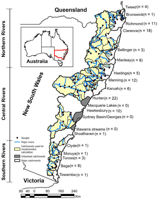
Figure 1.
Study catchments in coastal NSW. Red boundaries indicate NSW. n is the number of gauges used in each catchment. Urbanised catchments indicated in grey are excluded from subsequent analyses. For more information on the 116 study gauges, see Supplementary Table S1; Supplementary Data.
These hydro-geomorphology of the study catchments represent an interaction between geological, climatic, and anthropogenic controls that govern their hydrological characteristics and responses [61,68,69]. The geology of the region is characterised by, in the north, the New England Fold Belt that includes Devonian and Permian bedrocks, intruded by granite and granodiorite, and Tertiary basalt eruptions. From the mid-coast to the south the Sydney Basin geological unit includes near-horizontal sandstones and shales of Permian to Triassic age. All of these catchments drain East from an escarpment into rounded and rugged foothills that extend almost to the coast. Hence, over 80% of rivers in this setting are confined (valley bottom confinement of 85% to 100%) or partly-confined (valley bottom confinement between 10% and 85%) [70]. The lowland plans tend to be relatively short and very few truly alluvial, laterally-unconfined rivers occur. Laterally-unconfined rivers with valley bottom confinement of <10% are uncommon [70]. Where they do occur, they are dominantly single-channel, meandering, or low sinuosity rivers that flow over fine-grained and sand beds [70].
Across the study catchments, a diverse range of climates occur due to their vast geographical extent and varying topography [71]. Catchments in the north of the Northern Rivers Region experience a subtropical climate, whereas the remainder of the coastal catchments are temperate. The climate in these catchment sis dominated by ENSO and experiences extensive periods or drought or temperate conditions interspersed with intense rain and flooding [72]. Most major flooding in this region occurs after intense rain induced by east coast low pressure weather systems and rare tropical cyclones [73]. The escarpment dominated topography and confined/partly confined rivers accentuate the conditions for major flooding. In this region, interannual and interdecadal climatic and hydrological variability in eastern Australia results in some of the highest flood variability in the world, evidenced by high values of Flash Flood Magnitude Index (FFMI) and variations in annual runoff [68]. The Northern Rivers Region experiences higher average annual rainfall, more intense local storms, and greater seasonal variability [74]. Such conditions lead to sudden, intense rainfall events that can produce sharp, high peaked hydrographs [61]. The hydrological response in these catchments is often rapid due to both the intensity of the rainfall and the relatively low antecedent soil moisture in some cases. Rainfall in Central Rivers Region and Southern Rivers Region is generally lower in total amount, but more evenly distributed over time, often associated with frontal systems that track from the west [74]. The moderated rainfall and lower temperatures tend to produce less variable base flows and broader hydrograph shapes with less pronounced peak heights [61]. Three representative weather stations occur at Murwillumbah (Bray Park), Paterson (Tocal Automatic Weather Station—AWS), and Bega (Newtown Road) stations, which are located at the Northern Rivers, Central Rivers, and Southern Rivers regions, respectively. Mean annual rainfall at the Murwillumbah, Paterson and Bega stations are 1595 mm a−1, 948 mm a−1, and 863 mm a−1, with mean minimum and maximum monthly temperatures ranging from 14.5 to 25.8 °C, 12.1 to 24.2 °C, and 8.2 to 22.3 °C [75].
The coastal catchments of NSW are predominantly covered by native vegetation on hillslopes and contain vegetation associations including eucalyptus forests, temperate rainforests, and some rainforest [76,77]. Almost all valley bottoms and riparian zones were cleared of vegetation and wood within a few decades of European colonisation in the late 18th and early 19th centuries [69,78]. In many catchments, river geomorphology changed dramatically and soil erosion and sediment yields were high [79]. In recent decades geomorphic and vegetative recovery has been occurring and this is, in places, producing dramatic changes in flood hydrology and transmission times [61,73].
3. Materials and Methods
Flow and flood hydrograph records with one-hour time-steps of 116 gauges were used spanning a timeframe of 1908 to March 2022 (Supplementary Table S1). Streamflow time-series that are sourced from BoM [80] and WaterNSW [81] are high-quality with less than 5% uncertainty [82] and undergo QA/QC checks before release to the public. For example, gauge movements are calibrated to ensure consistency of data. Hence, the verification of input data quality is important before undertaking statistical analysis. Only in the Hunter catchment, some gauges have streamflow data extending back to the 1910s, while most of the gauges in this study have records beginning from the 1950s onward. Hence, the period of records in this study starts from the 1910s and covers several decades, a time during which there has been a concurrent processes of river ‘re-greening’ and geomorphic (structural) recovery [73,78]. A two-tier morphologically-defined flow and flood stage classification method was used to identify high flows and overbank floods using the method of Arash et al. [61] (Supplementary Figure S1). In this method, morphological thresholds for high flows and overbank floods were initially identified at each gauge station site using the surveyed cross-sections, then flow stage records were matched to the cross-sections at each gauge site. This study uses stage height hydrographs instead of discharge due to their broader availability, ease of comparison across streams, improved visualisation, alignment with stakeholder experiences, facilitation of rapid assessments, and practicality for communication and decision-making during flood events [83,84]. A high flow is defined as any flow that reaches a stage height that is between 50% lower and 5% higher than bankfull (hereafter termed near bankfull). These flows will inundate all instream geomorphic units and fill a considerable proportion of the channel. An overbank flood is any flow that exceeds a stage height of greater than 5% above bankfull. These flows are out-of-channel floods that inundate floodplains and surrounding areas. High flow is confined to the channel, whereas overbank floods exceed the bankfull level and spread onto the floodplain and are therefore influenced by both channel and valley morphology. In total, 2452 stage height hydrographs were extracted from the free access databases of BoM [80] and WaterNSW [81] [61]. The number of high flow and overbank flood hydrographs are 1584 and 868, respectively.
3.1. Hydrological Indicators
In this analysis, we use three hydrograph shape metrics as hydrological indicators (i.e., kurtosis—K (Equation (1)), skewness—S (Equation (2)), and rate-of-rise—RoR (Equation (3)) (See Table 1).
where µ refers to the arithmetic mean; µ3 corresponds to the third moment about the mean; µ4 corresponds to the fourth moment about the mean; Ϭ refers to the standard deviation; RoR refers to rate-of-rise (m h−1); Hp refers to the peak hydrograph stage (m); tp refers to the peak arrival time (h).

Table 1.
Definition of the hydrograph shape metrics measures used in the present study.
In hydrology, the kurtosis (K) of a stage hydrograph is often used to assess the degree of concentration or dispersion of flow stages around the average stage and whether the hydrograph has a more peaked or flat shape compared to a normal distribution. Leptokurtic (sharp peak and thick tails—kurtosis >3), mesokurtic (normal distribution—kurtosis of 3), and platykurtic (flat peak and thin tails—kurtosis <3) are several types of kurtosis. Skewness (S) measures the asymmetry of the distribution of stage values in a flow hydrograph. It quantifies the degree and direction of departure from symmetry or a normal distribution. Symmetrical distributions have a skewness of zero (no skew), right skew distributions have negative skewness, and left skew distributions have positive skewness. The RoR measures how quickly water stage rises during a flow or flood. RoR (m h−1) is calculated by dividing the peak hydrograph stage (m) by peak arrival time (h). In this study, the start time of a hydrograph is considered to be the onset of the precipitation event, which causes a rise in stage height above base flow. The end time is marked by the point when the peak hydrograph stage returns to base flow level. RoR (m h−1) is calculated by dividing the peak hydrograph stage (m) by peak arrival time (h). In this study, the start time of a hydrograph is considered to be the onset of the precipitation event, which causes a rise in stage height above baseflow. The end time is marked by the point when the peak hydrograph stage returns to baseflow level.
3.2. Catchment Morphometric Measures
Catchment morphometrics were calculated using watershed shapefiles, and a 30-m resolution digital elevation model (DEM) of Australia sourced from Geoscience Australia (GA) in the zonal statistics tool in ArcGIS Pro 3.2 [85]. The detailed processes are in Supplementary Figure S2. A database of the morphometric measures for each study catchment is published as S1 Data.
In regional-scale and catchment-scale studies, coarse resolution Digital Elevation Models (DEMs) (e.g., SRTM, ASTER, and ALOS) are commonly used because they provide sufficient resolution for the calculation and mapping of valley and catchment-scale morphology [86]. Such datasets are readily available and of broad coverage, allowing for wide-scale analysis for cross-comparative purposes. Of course, there will be limitations imposed for the measurement of some metrics in some situations. For example, Dd is difficult to measure in small, flat catchments with complex drainage features like ponds and lakes, and particularly in arid and semi-arid landscapes where low-order channels are often underestimated [38,87,88]. In other places, a DEM will force the integration of channel networks and, therefore, the integration of flow transmissions by drafting connected channels where they are not indeed present or functional. Elsewhere, the measurement of Vc may be limited by pixel size, particularly in first-order streams. If analyses are being undertaken in such areas, a user should make sensible decisions and carry out sufficient testing of DEMs before using them. In some cases, higher-resolution elevation models, GIS/RS techniques (e.g., hydrographic feature data models, stream burning), accompanied by field verification and measurement will be needed to accurately capture the river network [88,89,90,91]. Our study is undertaken in relatively larger, steeper catchments at catchment-to-regional scales, so a 30-m DEM is suitable for use.
The area draining into each gauge site ranges from 33 km2 to 17,780 km2. The gauge sites occur at elevations ranging from 83 m to 1348 m above sea level. Channel distance was calculated using the major and minor streamline shapefiles contained in the NSW River Styles database [70,92], together with the edit toolbox and calculate geometry tool in ArcGIS Pro 3.2. The distance between paired gauges ranges from 7 km to 359 km. These paired gauges refer to the subsequent gauging stations located along the same stream, from upstream to downstream.
In this analysis, we use five numeric morphometric measures: Er (Equation (4)), Rf (Equation (5)), Rh (Equation (6)), Dd (Equation (7)), and Sl (Equations (9) and (10)). We also used two categorical morphometric measures: Vc (Equation (8)), and Gp (Equation (11)) (See Table 2).
where Er refers to elongation ratio; A refers to the contributing catchment area (km2); At refers to the total catchment area (km2); L refers to the catchment length along its axis (km); Rf refers to the form factor; Rh refers to the relief ratio; H refers to the maximum catchment relief, which is the difference in elevation between the catchment mouth and the highest peak in the catchment (m); Dd refers to the drainage density (km km−2); ƩLs refers to the sum of channel lengths in a catchment (km); ƩLc refers to the sum of confined channel lengths (km); Ls refers to total channel length (km); Sli refers to the average longitudinal slope in 30-m interval; ΔHi refers to the difference between the elevation at 30-m interval (m); Δxi refers to reach length (m), which is assumed 30 m based on the DEM resolution; and Sl refers to the average longitudinal slope of the stream from the drainage divide to the gauge site.
Table 2.
Definition of the catchment morphometric measures used in the present study.
Catchments with an Er ratio closer to 1.0 and a high Rf are round and catchments with Er around 0.6 and a low Rf are elongate. A circular catchment means the distance from any point on the catchment boundary to the outlet is relatively uniform compared to an elongate catchment. Catchments with Rf close to 1 tend to have flashy flood regimes, while catchments with Rf closer to 0 tend to have lower flood intensities [30,93]. Catchments with high Sl and Rh tend to more accentuated topography and create flashy flow regimes [94]. Dd measures the potential of an area to generate discharge [95,96].
Gp can be positively correlated with Vc in some catchments. Vc is a straightforward, GIS-compatible metric that offers a relative measure of lateral valley scale/size. The extent to which flow is confined in a channel or on a valley bottom determines where flow expansion and contraction zones occur [97]. Vc classes are defined as: confined (Vc ≥ 90%), partly-confined (Vc = 10% to 90%) or laterally-unconfined (Vc < 10%) [98]. Confined valleys are expected to produce flashier hydrographs than laterally-unconfined valleys. Similar to Dd, Vc can be readily computed using GIS tools and widely available topographic datasets.
Gp is a categorical measure of whether the gauge is positioned in an upstream, midstream, or downstream location. Using the method of Arash et al. [61], if total drainage area to the total catchment area is less than 10% the gauge is classified as upstream; between 11% and 50% is classified as midstream, and more than 51% is classified as downstream. In upstream locations, gauges tend to be found in confined, steep valleys where hydrograph shape is expected to be more peaked (pointed shape), whereas gauges in downstream locations tend to occur in laterally-unconfined valleys hydrograph shape is expected to be more platykurtic. In this study, the number of gauges in upstream positions is 71, at midstream is 33, and at downstream is 12.
3.3. Statistical Analyses
All statistical analyses were performed by using Minitab version 22, and Python version 3. The first step in these analyses was the identification of median hydrograph shapes for high flows and overbank floods on a catchment scale by using the hydrographs in each catchment. The median hydrograph shape describes the variability of hydrograph shapes in a catchment as an indication of hydrological processes [20]. The median high flow and overbank flood hydrographs are the most closely matched the median values of K, S, and RoR in each individual catchment. These median hydrographs were selected for analysis. The total number of median high flow hydrographs is 99, and the total number of median overbank flood hydrographs is 62.
The subsequent analyses (Principal Components Analysis—PCA and Supervised Principal Components Analysis—SPCA) were conducted to determine correlations between hydrological characteristics and catchment morphometrics (Supplementary Figure S3). PCA was performed to determine the strength of correlation between hydrological characteristics and catchment morphometrics for both high flow and overbank flood types and then separately for each flood type. The PCA analysis employs the variance-based similarity matrices to identify new principal components in the dataset, where the data variance is maximised, thereby, PCA can reduce the number of indicators, while retaining most of the information. Also, the dominant morphometric control that explains the most variability in the hydrological data can be found. The number of selected principal components for selected further analyses was based on explaining at least 80% of the total variance of the original variables [23].
Before performing PCA, the data was standardised to prevent variables with larger variances, having a disproportionate influence on the PCA results. In this regard, the values of kurtosis, skewness, RoR, Er, Rf, Rh, Dd, and Sl were standardised using the Z-score method. The Z-score procedure was used to transform the variable by subtracting its mean and dividing by its standard deviation for each variable.
A K-means clustering method was used to define the number of clusters for high flow and overbank flood median hydrographs. The K-means method is commonly used as a partitional clustering technique that uses a clustering algorithm to define dissimilarity (or distance) between a data point and a cluster centroid to partition a dataset into a predetermined number of clusters. The common standard dissimilarity or distance metric used in K-means clustering method is Euclidean Distance. This metric is used to calculate the straight-line distance between each data point and each cluster centre in Euclidean space to assign data points to clusters and to optimise the positions of the cluster centres.
Elbow analysis was used to determine the optimal number of clusters to use in K-means clustering, with the aim of maintaining balance between compactness (within-cluster variance) and simplicity (number of clusters). All three hydrologic indicators (kurtosis, skewness and RoR) were used for elbow and K-means clustering methods. To evaluate the validity of the clustering method, three metrics of Silhoutte, Calinski-Harabasz and Davies-Bouldin scores were calculated for each number of clusters (i.e., [21]). Also, for each number of clusters, the K-means clustering algorithm was applied to the dataset. The resulting clusters were then visualised to confirm that data points were appropriately grouped. Once the clusters were identified for high flows and overbank floods, all median hydrographs within each cluster were plotted as ‘rainbow graphs’ (e.g., [20]), and the median and mean hydrograph of each cluster identified. The median hydrographs of each cluster are subsequently used as the median hydrograph shape in each cluster for further analyses.
One-way ANOVA analyses were independently conducted to test whether there is a significant difference between the means of three variables—kurtosis, skewness and RoR—across three clusters of high flow, and across three clusters of overbank flood. Each set of clusters (high flow and overbank flood) was analysed separately to determine if there were statistically distinct variations in these variables. The significance of the differences was assessed at a 95% confidence level, with a threshold of p-values ≤ 0.05. The labels for median hydrographs of high flow clusters and overbank flood clusters were adopted from Brunner et al. [20], as 1. flashy, 2. intermediate, and 3. broad.
To determine the mix of controls operating on each of the high flow and overbank clusters, and to establish the dominance or percentage of contribution of each to the relationship, SPCA was used. SPCA can be used on categorical data (in this case cluster labels) and can be used to reduce the variables that describe the data and discriminate between clusters [99,100]. This means that the principal components generated from SPCA analysis are not just about capturing the maximum variance among features but also about being relevant to the prediction of a response variable. This makes SPCA particularly useful in this classification task where the response variable is categorical (cluster labels). To capture over 50% of variance, both PC1 and PC2 were considered. Then, the PC1 weights and PC2 weights for each cluster were used in the SPCA analysis, and the percentage of contribution of each control in PC1 and PC2 was calculated. The weight for PC1 was calculated by considering both the variance in the catchment controls, and the relationship of these predictors with the cluster labels. PC2 was calculated in the same way as PC1 to make sure that the important variations in the data that are not visible in PC1 are also captured. However, the PC1 and PC2 in standard PCA are calculated by achieving the highest variance in the catchment controls, regardless of how strongly they are related to the cluster labels.
In this study, dominant catchment morphometric controls for high flow and overbank floods are those which explain the highest cumulative variance (more than 60%) explained by both PC1 and PC2. Hence, the controls with the highest contribution scores and the percentage of contribution (more than 60%), when considering both PC1 and PC2, are considered dominant. The contribution score was calculated by summing the absolute values of the loadings of catchment morphometric controls across both PC1 and PC2 [101]. The absolute value captures the size of the contribution regardless of whether it is positive or negative, which is more essential in the interpretation of PCA analysis results than the direction of its influence.
4. Results
4.1. PCA and Standardisation Analysis Results
4.1.1. High Flows
In the eigen analysis of the correlation matrix, the eigenvalues of PC1 to PC7 for high flow median hydrographs were calculated, and the PC1 to PC4 with eigenvalues greater than one were selected for further analyses (Supplementary Figure S4 and Supplementary Tables S2 and S3). PC1 is strongly and positively correlated with S, K, Er, Rf, and Rh with a loading of 0.4. Gp and RoR are negatively correlated to PC1, and Dd, Vc, and Sl are positively correlated to PC1. PC2 is strongly and positively correlated with Er and Rf with a loading of 0.45, and PC2 is strongly and negatively correlated with Vc, Sl and K with a loading of −0.35. Dd, RoR and Gp are positively correlated with PC2, and S and Rh are negatively correlated with PC2.
The PCA biplot for median high flow hydrographs indicates that Er and Rf are positively correlated and each of them are positively correlated with Dd (Figure 2 and Supplementary Table S4). The correlation matrix from PCA biplot analysis for median high flow hydrographs shows Vc and Sl are strongly correlated, and they are each negatively correlated with Dd, Er and Rf. In this PCA biplot, the small angle between RoR and Gp suggests that they are positively correlated. Also, there is a strong positive correlation between K, S, and Rh. PCA analysis results indicate that 99% of the variance can be captured by using only 8 components instead of 10 (Supplementary Table S2). Given that Er is strongly correlated with Rf, and Sl with Vc, only two of these variables were for subsequent statistical analyses (clustering): Er (in place of Rf) and Sl (instead of Vc).
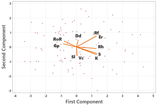
Figure 2.
PCA biplot for representative high flow hydrographs (count: 99). In this figure, K refers to kurtosis, S refers to skewness, RoR refers to rate-of-rise, Rf refers to form factor, Vc refers to valley confinement at the gauge, Er refers to elongation ratio, Dd corresponds to drainage density, Sl refers to average longitudinal slope upstream of the gauge, Gp corresponds to gauge position in the catchment, and Rh refers to catchment relief.
4.1.2. Overbank Floods
The PCA biplot for median overbank flood hydrographs is shown in Figure 3. In the eigen analysis of the correlation matrix, the eigenvalues of PC1 to PC10 for overbank floods were calculated (Supplementary Figure S5 and Supplementary Table S5). PC1 to PC5 with eigenvalues higher than one were retained (Supplementary Table S5). PC1 is strongly and positively correlated with K, S, Er and Rf (loading of 0.4), and positively correlated with Rh, Dd, Vc and Sl. Rh and RoR are negatively correlated with PC1 (Supplementary Table S6 and S7). PC2 is strongly and positively correlated with S, K, Vc and Sl, and strongly and negatively correlated with Er, Rf and RoR. Gp is positively correlated with PC2, and Rh and Dd are negatively correlate with PC2.
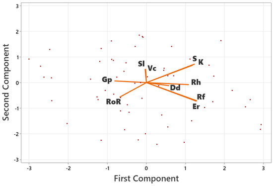
Figure 3.
PCA biplot for representative overbank flood hydrographs (count: 62). In this figure, K refers to kurtosis, S refers to skewness, RoR refers to rate-of-rise, Rf refers to form factor, Vc refers to valley confinement at the gauge, Er refers to elongation ratio, Dd corresponds to drainage density, Sl refers to average longitudinal slope upstream of the gauge, Gp corresponds to gauge position in the catchment, and Rh refers to catchment relief.
The small angle between K-S, Er-Rf, and Vc-Sl pairs show that these variables are positively correlated (Figure 3 and Supplementary Table S6). The correlation matrix from PCA biplot analysis for median overbank flood hydrographs shows Rh and Dd are positively correlated and each of them is negatively correlated with Gp and RoR. Also, K, S, Rf, and Er are negatively correlated with Gp and RoR. There is no correlation between the Vc-Sl pair, and other variables. Similar to high flows, to prevent duplication of morphometrics that measure similar characteristics, Er and Sl (instead of Rf and Vc) were selected for further analysis.
4.2. Elbow Analysis and K-Mean Clustering Method for Representative High Flow and Overbank Flood Hydrographs
The three hydrological indicators, K, S, and RoR of median high flow and overbank flood hydrographs were used as inputs to the clustering method. K-means clustering method was used to test for 2 to 10 clusters. In the K-means clustering method, the mean-with cluster sum of squares of 2 to 10 clusters was calculated (Supplementary Tables S8–S10 and Supplementary Tables S11–S13). The mean-within cluster sum of squares between 3 and 4 clusters has the lowest variability, and the calculated Silhoutte, Calinski-Harabasz and Davies-Bouldin scores for 3 and 4 clusters were the same scores, which indicates that either of them can be used. The K-means clustering algorithm was applied independently to partition the data into 3 and 4 clusters, with the results of each plotted for analysis. The results revealed that with 4 clusters, one group contained fewer than 5 data points, while the others each had more than 15 data points. In contrast, when using 3 clusters, the distribution of data points across the groups was more balanced and relatively equal compared to 4 clusters. Hence, for subsequent analysis, 3 clusters were selected.
The K-means algorithm successfully segmented median high flow hydrographs into three distinct clusters based on K, S, and RoR. Similarly, three clusters of K-means were identified for median overbank flood hydrographs. Data visualisation was undertaken to validate the accuracy of K-means clustering method in terms of the identification of overlaps or gaps between clusters, the examination of the size and balance of the clusters, and the identification of outliers. In this regard, the K, S, and RoR for the three high flow and overbank flood clusters are plotted in three-dimensional plots in (Figure 4a,b), and the statistics of these analyses for median high flow and overbank flood hydrographs are shown in Supplementary Tables S8–S10 in for high flows, and in Supplementary Tables S11–S13, for overbank flows. For ease of communication herein, Cluster 1 hydrographs are classed as flashy, Cluster 2 as intermediate, and Cluster 3 as broad.
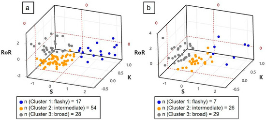
Figure 4.
Three-dimensional plot showing the K, S, and RoR values of different clusters for (a) representative high flow hydrographs (Cluster 1: flashy, Cluster 2: intermediate, and Cluster 3: broad), and (b) overbank flood hydrographs (Cluster 1: flashy, Cluster 2: intermediate, and Cluster 3: broad). The n values indicate the number of representative high flow hydrographs and representative overbank flood hydrographs in each cluster. In this figure, K refers to kurtosis, S refers to skewness, RoR refers to rate-of-rise.
For high flow hydrographs, the means of standardised K, standardised S, and standardised RoR for median flashy (n = 17), intermediate 2 (n = 54), and broad 3 (n = 28) clusters are shown in Figure 5a–c. A one-way ANOVA at a 95% confidence level (p-value ≤ 0.05) was used to test whether there is a significant difference in K, S, and RoR between the three clusters (Supplementary Tables S14–S25). The one-way ANOVA test shows there is a significant difference in K, S, and RoR for the three different clusters (p-value ≤ 0.05). Furthermore, the values of R2 across all clusters is higher than 68%, which indicates that ANOVA model is appropriate in explaining variations in K, S, and RoR.
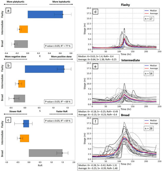
Figure 5.
(a) standardised K, (b) standardised S, and (c) standardised RoR characteristics for each cluster of representative high flow hydrographs, with one-way ANOVA results. (d–f) Three clusters of representative high flow hydrograph shapes for coastal catchments of NSW are shown in grey scale (1. flashy, 2. intermediate and 3. broad). The median hydrograph shape per cluster is shown in blue, and the mean hydrograph shape per cluster is shown in red. The n values indicate the number of representative high flow hydrographs in each cluster. In this figure, K refers to kurtosis, S refers to skewness, RoR refers to rate-of-rise.
To display the differences in the median high flow hydrograph shape by cluster, median hydrographs for all three clusters, their median, and mean shape are shown in Figure 5d–f. The median hydrograph is the most closely matched the median values of K, S, and RoR in each cluster. Similarly, the mean hydrograph corresponds most closely to the mean values of K, S, and RoR in each cluster. Flashy hydrographs are characterised by the highest K, and S, and a low RoR compared with other clusters. These hydrographs have steep rising and falling limbs, a low peak stage height, and right-tailed skewed. Broad hydrographs are characterised by the lowest K, and S, and the highest RoR. These hydrographs exhibit steeper rising and falling limbs, are more peaked, and left-tailed skewed. Broad hydrographs have more skew, have a faster rate of rise, followed by a gradual decline, indicating slower drainage processes. Flashy hydrographs, on the other hand, have less skew and a slower rise, with a sharp recession after the peak, reflecting rapid runoff. Intermediate hydrographs are charactered by a higher K and S and lower RoR compared to broad hydrographs. This means that intermediate hydrographs have less steep rising and falling limbs, are less peaked, and more right-tailed skewed compared to flashy hydrographs. The median stage height value for broad high flow hydrographs (~10 m) is higher than for flashy (~5 m) and intermediate (~5 m) hydrographs.
For overbank flood hydrographs, the means of standardised K, standardised S, and standardised RoR for median flashy (n = 7), intermediate (n = 26), and broad 3 (n = 29) clusters are shown in Figure 6a–c. To test the significance in the means of K, S, and RoR between three clusters, a one-way ANOVA at a 95% confidence level (p-value ≤ 0.05) was used (Supplementary Tables S26–S37). The values of R2 for K and S are higher than 71%, which indicates that the ANOVA model is appropriate in explaining the variations in K, and S. However, the R2 for RoR is 39%, which shows that the ANOVA model is not explaining all variations in RoR. RoR is important for differentiating between flashy and intermediate relative to broad hydrographs, because RoR of broad hydrographs is much higher than others. K and S help to differentiate between broad and intermediate hydrographs. Hence, all these indicators (K, S and RoR) are required for clustering of the median hydrographs.
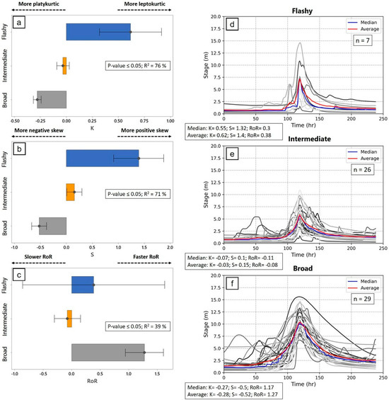
Figure 6.
(a) standardised K, (b) standardised S, and (c) standardised RoR characteristics for each cluster for representative overbank flood hydrographs with one-way ANOVA results. (d–f) Three clusters of representative overbank flood hydrographs shapes for coastal catchments of NSW (flashy, intermediate and broad) are shown in grey scales. The median hydrograph shape per cluster is shown in blue, and the mean hydrograph shape per cluster is shown in red. The n values indicate the number of representative overbank flood hydrographs in each cluster. In this figure, K refers to kurtosis, S refers to skewness, RoR refers to rate-of-rise.
Median overbank flood hydrographs for all three clusters, their median, and mean shape are shown (Figure 6d–f). The median hydrograph is the most closely matched the median values of K, S, and RoR in each cluster. Similarly, the mean hydrograph corresponds most closely to the mean values of K, S, and RoR in each cluster. Flashy hydrographs are characterised by the highest K, S, and low but highly variable RoR. Flashy hydrographs exhibit steep rising and falling limbs, are more peaked, and right-tailed skewed. However, the peak stage height is variable and ranges between 1.5 and 15 m. Intermediate hydrographs are characterised by a lower K, S, and RoR, having less steep rising and falling limbs, being less peaked, and more left-tailed skewed compared to flashy hydrographs. Broad hydrographs are charactered by a higher RoR, and the lowest K and S compared to flashy and intermediate hydrographs. This means that broad hydrographs have less steep rising and falling limbs, are more less and more left-handed skewed. The median stage height value for broad overbank hydrographs (~10 m) is higher than for flashy (~7.5 m) and intermediate (~5.5 m) hydrographs.
4.3. Regional- and Catchment-Scale Distribution of Different Types of Representative High Flow and Overbank Flood Hydrographs
The results of the count of median high flow and overbank flood hydrographs at catchment scale and regional scale are summarised in Figure 7 and Supplementary Tables S38 and S39. For high flows (Figure 7a), flashy hydrographs are most common in the Northern Rivers (25%), followed by the Southern Rivers (17%), and Central Rivers (10%). The Richmond, Macleay, and Hunter catchments have the highest number of flashy hydrographs (count > 4). Intermediate high flow hydrographs make up the greatest proportion across all regions, being highest in the Central Rivers (60%), followed by Southern Rivers (58%) and Northern Rivers (45%). Intermediate high flow hydrographs are found in almost all catchments, expect for Clyde and Towamba, with the Hunter having the highest count (n = 10). Broad hydrographs are more common in the Northern Rivers (30%) and Central Rivers (30%) than in the Southern Rivers (25%), with the highest number found in the Hunter, Richmond, Clarence, and Manning catchments (count > 4).
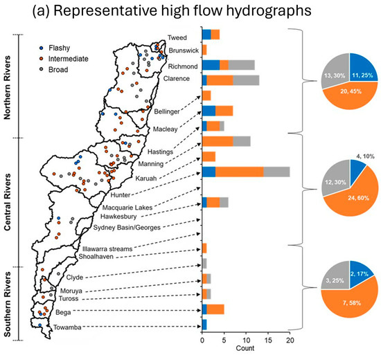
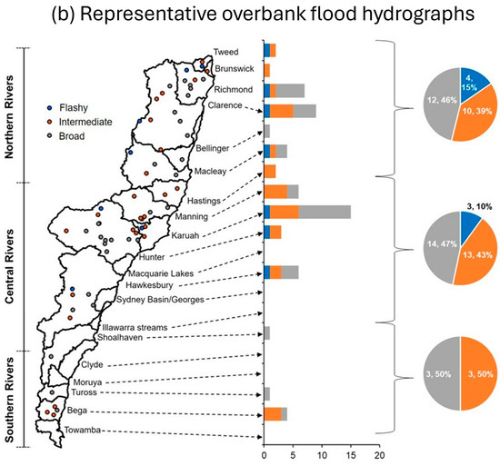
Figure 7.
Cluster count summarised for each catchment, and region (Northern Rivers, Central Rivers and Southern Rivers) for (a) representative high flow hydrographs (flashy, intermediate and broad), and (b) representative overbank flood hydrographs (flashy, intermediate and broad).
For overbank floods (Figure 7b), the number of flashy hydrographs is low in the Northern Rivers (15%), Central Rivers (10%), and Southern Rivers (absent; 0%). Intermediate hydrographs are highest in the Southern Rivers (50%), followed by Central Rivers (43%) and Northern Rivers (39%). There are at least two intermediate hydrographs in each of the Hunter, Manning, Clarence, Richmond, and Bega catchments. Broad hydrographs make up the greatest proportion across all regions, being highest in the Southern Rivers (50%), followed by Central Rivers (47%) and Northern Rivers (46%), with the Karuah catchment having the highest count (n = 10).
Based on the count of median high flow and overbank flood hydrographs in each catchment (Supplementary Table S39), many catchments across the region experience intermediate high flow hydrographs, and intermediate overbank flood hydrographs. On average, catchments that experience the highest number of intermediate high flow hydrographs also experience the highest number of intermediate overbank flood hydrographs. However, intermediate high flow hydrographs and broad overbank flood hydrographs are the most frequent type of floods in the Shoalhaven Catchment. There are no available recorded overbank flood hydrographs in some catchments in the Southern Rivers Region, such as the Clyde, Moruya, and Towamba catchments.
4.4. SPCA Analysis to Identify the Mix and Dominance of Catchment Morphometric Controls on Each Flood Type Cluster
SPCA was used to identify the dominant catchment morphometric controls on flood hydrograph shape (Supplementary Figures S6 and S7, and Supplementary Tables S40–S45. For both high flow and overbank floods, PC1 explains 35% of variance and PC2 explains nearly 25% of variance, thereby both PC1 and PC2 eigenvalues were used to identify the dominant controls for high flows and overbank floods.
Figure 8 shows the SPCA biplot for the median hydrographs of high flow clusters, and overbank flood clusters. The distribution of datapoints (median hydrographs) are not the same thereby the datapoints with each cluster are correlated with different vectors (controls) for high flows and overbank floods. The distances between the cluster centroids are distinct, and regardless of some overlaps between clusters, data points within the same cluster are relatively close to each other. Hence, the clusters are statistically and visually different to each other, which was also shown in Figure 4. Across all flood types and clusters, Er and Rh are positively correlated, and each of them are negatively correlated with Gp (Figure 8a,b). Dd and Sl are negatively correlated, and there is no correlation among them with Er, Rh, and Gp.
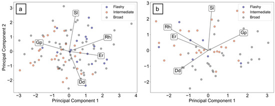
Figure 8.
SPCA biplot for the median hydrographs of (a) high flow clusters, and (b) overbank flood clusters. In this figure, Er refers to elongation ratio, Dd corresponds to drainage density, Sl refers to average longitudinal slope upstream of the gauge, Gp corresponds to gauge position in the catchment, and Rh refers to catchment relief.
Table 3 shows the PC1 weights, PC2 weights, and percentage of contribution of each control in PC1 and PC2 based on the SPCA analyses, as indicators of relative dominance for high flow and overbank floods. For high flow hydrographs, the mix of morphometric controls that best explain variations across all clusters are Dd, Rh and Sl (cumulative contributions more than 60%). For flashy hydrographs, the dominant controls are Er, Sl and Dd; broad, the dominant controls are Rh, Sl and Gp; and intermediate, the dominant controls are Dd, Rh and Sl, respectively. The contribution score of Er is only 15% for both broad and intermediate hydrographs, and the contribution score of Gp is 18% for flashy and intermediate hydrographs.
Table 3.
The PC1 and PC2 weights of Er, Rh, Dd, Sl, and Gp (percentage of contribution of each control in PC1, as an indicator of percentage of dominance shown in parentheses) based on the SPCA analyses for high flow clusters, and overbank flood clusters. In this table, Er refers to elongation ratio, Dd corresponds to drainage density, Sl refers to average longitudinal slope upstream of the gauge, Gp corresponds to gauge position in the catchment, and Rh refers to catchment relief.
For overbank flood hydrographs, the dominant mix of morphometric controls that explain variations across all clusters are Er, Dd, and Rh (or Gp) at 67%, followed by Gp at 18% and Sl at 15%. Either Rh or Gp can be used as their scores is nearly the same. For flashy hydrographs, Rh and Sl with a cumulative contribution score of 57% is the best mix of controls, and Er, Dd and Gp have minor impacts in explaining the variation in the flood behaviour of flashy hydrographs. For intermediate and broad hydrographs, the mix of Er and Dd controls each with a contribution of between 20% to 30% are the dominant controls, and for intermediate, Rh is the third control with a contribution of nearly 20%. The contribution score of Sl is less than 17% for both intermediate and broad hydrographs. Based on the results, Gp has a minor impact on the variation in the flood behaviour across all clusters of overbank flood hydrographs.
Overall, Rh and Dd are the dominant controls on hydrograph shape with contributions more than 42% across all flood types and clusters. For high flow, Sl and for overbank floods, Er are other dominant controls that together with Rh and Dd can explain more than 65% of variation in the flood behaviour across all clusters of high flow and overbank flood hydrographs.
5. Discussion
5.1. Identification of Different Hydrograph Shapes, and Hydrograph Types
In this study a hydro-morphic catchment classification was used to characterise and categorise catchments based on both hydrological and geomorphological attributes. When robust, hydro-morphic catchment classification has a wide range of applications, including land use planning, water resource management, and environmental monitoring [11,102,103,104,105].
The results of K-means clustering approach based on kurtosis (K), skewness (S), and rate-of-rise (RoR) of the catchment-specific sets of median (median) hydrographs revealed three statistically distinct clusters of high flow hydrographs, and three clusters of overbank flood hydrographs (Figure 4, Figure 5 and Figure 6). The hydrographs belonging to these clusters have flashy, intermediate and broad shapes (e.g., [20]). These clusters are distinctive in terms of magnitude, time-to-peak and distribution. Also, the clustering results indicate the hydrological diversity of catchments in the coastal NSW with median hydrograph shapes occurring in each catchment (Figure 7).
Flashy high flow hydrographs and flashy overbank flood hydrographs have steep rising and falling limbs, are more peaked and are right-tail skewed. Across high flow and overbank flood clusters, flashy hydrographs mostly occur in catchments in the Northern Rivers and Central Rivers Regions that have a very high slope, high drainage density and are relatively round [27,28,106].
Broad high flow hydrographs and broad overbank flood hydrographs have a high peak stage, have less steep rising and falling limbs, are less peaked, and are left-tail skewed. These hydrographs occur in round catchments that are large in size, have steep slope and a high drainage network density, such as Hunter, Richmond, Clarence, Manning and Karuah catchments in the Central Rivers Region [28,107,108].
Intermediate high flow hydrographs and intermediate overbank flood hydrographs have a relatively similar high peak stage, but broader distribution compared to flashy hydrographs. These hydrographs are the most frequent and they occur in catchments with a relatively lower slope, lower drainage density, and more elongate shape, such as Hunter, Manning, Hasting and Clarence catchments [20,28,30,108].
5.2. Identification of the Mix and Dominance of Catchment Morphometric Controls on Flood Behaviour
Hydrological behaviour can vary considerably in catchments and regions with a different mix of morphometric characteristics [9,10,49,109]. However, using the analysis presented in this paper, it is possible to determine the dominant (i.e., the best explanatory) controls on hydrograph shape in individual catchments and across a region based on a refined suite of morphometric parameters. This approach can be used as one way to explain the hydrological behaviour of catchments (i.e., See [12,23,39,45]).
Our results suggest that hydrological behaviours of high flows and overbank floods are controlled by different mixes of catchment size, shape, topography and drainage network characteristics [9,10,95,110]. The topographic characteristics of catchments (i.e., relief and longitudinal slope, Rh and Sl in this study) are commonly among the dominant controls for all high flow and overbank flood hydrographs, excluding broad overbank floods. Drainage network structure (i.e., drainage density, Dd in this study) is also an important control on flashy and intermediate high flows, and intermediate and broad overbank floods, while catchment size (i.e., gauge position in the network, Gp in this study) influences broad high flows. Catchment shape (i.e., elongation ratio, Er in this study) influences broad overbank floods, and catchment shape characteristics are dominant for flashy high flows, and intermediate and broad overbank floods. Generally, topographic controls are more useful for differentiating the hydrological behaviour of high flows relative to overbank floods.
Overall, across all clusters of high flow and overbank floods, topographic (Rh or Sl) and drainage network structure (Dd) characteristics of catchments are commonly the dominant controls, accounting for more than 42% of the variance measured (Figure 9). Also, the behaviour of flows that reach to bankfull (high flows) is influenced more by some local-scale controls, such as channel slope (Sl) rather than catchment relief (Rh). There are other local-scale controls operating on high flows, such as channel roughness, size, shape, planform etc. that have not been tested here [18,25,111,112,113]. Future work to broaden the range of local-scale controls operating on high flows would improve the interpretation of regional-scale patterns (and clusters) of high flow behaviour [16,34,41,114,115].
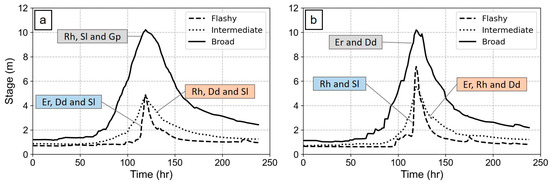
Figure 9.
The representative (median) hydrograph shape of flashy, intermediate and broad hydrographs for (a) high flows, and (b) overbank floods. The dominant controls based on the SPCA analyses are noted in the box for each hydrograph type.
5.3. The Potential Application of a Hydro-Morphic Classification of Catchments
We acknowledge that our method is best suited for use in medium sized catchments where climatic and hydro-geomorphic characteristics are relatively uniform and where there is a reasonable distribution and availability of gauge data. It will also work well in landscapes and catchments that are slightly dissected, and where rivers are dominantly confined or partly confined and do not contain a wide array of floodplain and alluvial river types. In these situations, it can provide a relatively cost- and time-effective analysis that can be used by hydrologists to do a high-level analysis of spatial patterns of flood behaviour (See Figure 7, [44,116]), and identify drainage network configuration and structural landscape controls that may be having a significant effect on flood behaviour [93,117,118]. Given that hydrograph shape integrates different processes occurring in catchments at different scales, a hydro-morphic classification of catchments can be used to identify “type basins”. These “type basins” could then be correlated with neighbouring catchments with like-for-like morphometric characteristics that may have scarce to null hydrological data as a basis to infer the hydrological functioning of these systems during floods [21,41,45,55,62]. This “reverse mode use” could be particularly useful in areas of the world where there is a lack of robust hydrological data. Additionally, such insights could be used to interpolate and extrapolate input data for hydrological models in ungauged catchments with like-morphometric characteristics and the development of cluster or class-specific hydrological models [11,21,41,62,107,119].
For flood management, this hydro-morphic classification and method can be used across catchments and regions (see Figure 7) to help managers understand flood behaviour in their catchments and to identify the catchments and regions where flood management is possible [19,60,61,120,121]. Such analysis identifies the landscape-imposed controls (i.e., catchment size or slope) and core characteristics of flood behaviour that cannot readily be manipulated. Therefore, for river managers, this understanding helps to determine what can (and cannot) be realistically manipulated in flood risk management [102,122,123,124]. Further work is required to determine the extent to which factors such as riparian revegetation and changes in land cover can be manipulated in these systems to have some effect on flood behaviour and mitigation [111,113].
6. Conclusions
This study presents a hydro-morphic catchment classification for coastal catchments of NSW, Australia. It uses 1584 high flow (near bankfull) hydrographs, and 868 overbank flood hydrographs to determine if there are statistically distinct clusters of hydrograph shapes in these systems. Three clusters (flashy, intermediate and broad) for high flow hydrographs and the same for overbank flood hydrographs were identified. These clusters are related to a refined suite of catchment-scale morphometric controls to identify the dominant controls on high flow and overbank flood behaviour. Topographic controls (i.e., relief and longitudinal slope) were dominant for almost all high flow and overbank flood hydrographs, while drainage network structure plays an important role for flashy and intermediate high flows, and intermediate and broad overbank floods. Catchment shape is a key control for broad overbank floods, although catchment shape characteristics influenced flashy high flows, and intermediate and broad overbank floods. Overall, topographic controls were more useful for differentiating the hydrological behaviour of high flows relative to overbank floods. This hydro-morphic catchment classification and method can aid practitioners to understand flow and flood behaviour in catchments, to select and develop class-specific hydrological models and extrapolate them to ungauged catchments, and to aid prediction of hydrological responses in catchments for use in flood risk analysis and management.
Supplementary Materials
The following supporting information can be downloaded at: https://www.mdpi.com/article/10.3390/geosciences15040141/s1.
Author Contributions
Conceptualization, A.M.A., K.F. and T.J.R.; Methodology, A.M.A.; Formal Analysis, A.M.A.; Investigation, A.M.A., K.F. and T.J.R.; Resources, K.F.; Data Curation, A.M.A.; Writing—Original Draft Preparation, A.M.A. and K.F.; Writing—Review & Editing, A.M.A., K.F., and T.J.R.; Visualization, A.M.A.; Supervision, K.F. and T.J.R.; Project Administration, A.M.A. and K.F.; Funding Acquisition, K.F. and T.J.R. All authors have read and agreed to the published version of the manuscript.
Funding
This research was funded by an Australian Research Council Linkage grant (LP190100314) led by KF with industry partners Landcare Australia and Hunter-Central Rivers Local Land Services. AA is supported by an Australian Commonwealth Government International Research Training Program (iRTP) and Macquarie University Higher Degree Research Funds.
Data Availability Statement
The original contributions presented in this study are included in the article/Supplementary Material (S1 Data). Further inquiries can be directed to the lead author.
Conflicts of Interest
The authors declare no conflicts of interest.
References
- Horton, R.E. Erosional development of streams and their drainage basins; hydrophysical approach to quantitative morphology. Geol. Soc. Am. Bull. 1945, 56, 275–370. [Google Scholar] [CrossRef]
- Leopold, L.B.; Wolman, M.G.; Miller, J.P. Fluvial processes in geomorphology. Dover Publications, Inc.: New York, NY, USA, 1964. [Google Scholar]
- Schumm, S.A.; Lichty, R.W. Channel widening and flood-plain construction along Cimarron River in southwestern Kansas. U.S. Geol. Surv. Prof. Pap. 1963, 352-D, 71–88. [Google Scholar] [CrossRef]
- Strahler, A. Quantitative Geomorphology of Drainage Basins and Channel Networks. In Handbook of Applied Hydrology; Chow, V., Ed.; McGraw Hill: New York, NY, USA, 1964; pp. 439–476. [Google Scholar]
- Hack, J.T. Studies of longitudinal stream profiles in Virginia and Maryland. Geol. Soc. Am. Bull. 1957, 68, 124–141. [Google Scholar]
- Chorley, R.J. (Ed.) The drainage basin as the fundamental geomorphic unit. In Introduction to Physical Hydrology; Routledge: London, UK, 1969. [Google Scholar]
- Howard, A.D. Drainage analysis in geologic interpretation: A summation. Am. Assoc. Pet. Geol. Bull. 1967, 51, 2246–2259. [Google Scholar] [CrossRef]
- Gregory, K.J.; Walling, D.E. Report: Fluvial Processes in Small Instrumented Watersheds in the British Isles. Area 1973, 5, 297–302. [Google Scholar]
- Benda, L.; Andras, K.; Miller, D.; Bigelow, P. Confluence effects in rivers: Interactions of basin scale, network geometry, and disturbance regimes. Water Resour. Res. 2004, 40, W05402. [Google Scholar] [CrossRef]
- Benda, L.E.E.; Poff, N.L.; Miller, D.; Dunne, T.; Reeves, G.; Pess, G.; Pollock, M. The network dynamics hypothesis: How channel networks structure riverine habitats. BioScience 2004, 54, 413–427. [Google Scholar] [CrossRef]
- Wagener, T.; Sivapalan, M.; Troch, P.; Woods, R. Catchment Classification and Hydrologic Similarity. Geogr. Compass 2007, 1, 901–931. [Google Scholar] [CrossRef]
- Ali, G.; Tetzlaff, D.; Soulsby, C.; McDonnell, J.J.; Capell, R. A comparison of similarity indices for catchment classification using a cross-regional dataset. Adv. Water Resour. 2012, 40, 11–22. [Google Scholar] [CrossRef]
- Brunner, M.I.; Viviroli, D.; Sikorska, A.E.; Vannier, O.; Favre, A.C.; Seibert, J. Flood type specific construction of synthetic design hydrographs. Water Resour. Res. 2017, 53, 1390–1406. [Google Scholar] [CrossRef]
- Jehn, F.U.; Bestian, K.; Breuer, L.; Kraft, P.; Houska, T. Using hydrological and climatic catchment clusters to explore drivers of catchment behaviour. Hydrol. Earth Syst. Sci. 2020, 24, 1081–1100. [Google Scholar] [CrossRef]
- Singh, P.K.; Kumar, V.; Purohit, R.C.; Kothari, M.; Dashora, P.K. Application of principal component analysis in grouping geomorphic parameters for hydrologic modeling. Water Resour. Manag. 2008, 23, 325–339. [Google Scholar] [CrossRef]
- Sawicz, K.; Wagener, T.; Sivapalan, M.; Troch, P.A.; Carrillo, G. Catchment classification: Empirical analysis of hydrologic similarity based on catchment function in the eastern USA. Hydrol. Earth Syst. Sci. 2011, 15, 2895–2911. [Google Scholar] [CrossRef]
- Merz, R.; Blöschl, G. A regional analysis of event runoff coefficients with respect to climate and catchment characteristics in Austria. Water Resour. Res. 2009, 45, W01405. [Google Scholar] [CrossRef]
- Ley, R.; Casper, M.C.; Hellebrand, H.; Merz, R. Catchment classification by runoff behaviour with self-organizing maps (SOM). Hydrol. Earth Syst. Sci. 2011, 15, 2947–2962. [Google Scholar] [CrossRef]
- Sikorska, A.E.; Viviroli, D.; Seibert, J. Flood-type classification in mountainous catchments using crisp and fuzzy decision trees. Water Resour. Res. 2015, 51, 7959–7976. [Google Scholar] [CrossRef]
- Brunner, M.I.; Viviroli, D.; Furrer, R.; Seibert, J.; Favre, A.-C. Identification of Flood Reactivity Regions via the Functional Clustering of Hydrographs. Water Resour. Res. 2018, 54, 1852–1867. [Google Scholar] [CrossRef]
- Rao, A.R.; Srinivas, V.V. Regionalization of watersheds by hybrid-cluster analysis. J. Hydrol. 2006, 318, 37–56. [Google Scholar] [CrossRef]
- Zhang, M.; Liu, N.; Harper, R.; Li, Q.; Liu, K.; Wei, X.; Ning, D.; Hou, Y.; Liu, S. A global review on hydrological responses to forest change across multiple spatial scales: Importance of scale, climate, forest type and hydrological regime. J. Hydrol. 2017, 546, 44–59. [Google Scholar] [CrossRef]
- Kuentz, A.; Arheimer, B.; Hundecha, Y.; Wagener, T. Understanding hydrologic variability across Europe through catchment classification. Hydrol. Earth Syst. Sci. 2017, 21, 2863–2879. [Google Scholar] [CrossRef]
- Wolman, M.G.; Miller, J.P. Magnitude and Frequency of Forces in Geomorphic Processes. J. Geol. 1960, 68, 54–74. [Google Scholar] [CrossRef]
- Phillips, J.D.; Slattery, M.C. Downstream trends in discharge, slope, and stream power in a lower coastal plain river. J. Hydrol. 2007, 334, 290–303. [Google Scholar] [CrossRef]
- Singh, V.P. (Ed.) Handbook Of applied Hydrology, 2nd ed.; McGraw-Hill Education: New York, NY, USA, 2016; pp. 439–476. [Google Scholar]
- Moussa, R. On morphometric properties of basins, scale effects and hydrological response. Hydrol. Process. 2003, 17, 33–58. [Google Scholar] [CrossRef]
- Charlton, R. Fundamentals of Fluvial Geomorphology; Routledge: London, UK, 2007. [Google Scholar]
- Kvočka, D.; Ahmadian, R.; Falconer, R.A. Flood inundation modelling of flash floods in steep river basins and catchments. Water 2017, 9, 705. [Google Scholar] [CrossRef]
- Abdulkareem, J.H.; Pradhan, B.; Sulaiman, W.N.A.; Jamil, N.R. Quantification of runoff as influenced by morphometric characteristics in a rural complex catchment. Earth Syst. Environ. 2018, 2, 145–162. [Google Scholar] [CrossRef]
- Gaál, L.; Szolgay, J.; Kohnová, S.; Parajka, J.; Merz, R.; Viglione, A.; Blöschl, G. Flood timescales: Understanding the interplay of climate and catchment processes through comparative hydrology. Water Resour. Res. 2012, 48, W04511. [Google Scholar] [CrossRef]
- Nied, M.; Schröter, K.; Lüdtke, S.; Nguyen, V.D.; Merz, B. What are the hydro-meteorological controls on flood characteristics? J. Hydrol. 2017, 545, 310–326. [Google Scholar] [CrossRef]
- Tarasova, L.; Merz, R.; Kiss, A.; Basso, S.; Blöschl, G.; Merz, B.; Viglione, A.; Plötner, S.; Guse, B.; Schumann, A.; et al. Causative classification of river flood events. Wiley Interdiscip. Rev. Water 2019, 6, e1353. [Google Scholar] [CrossRef]
- Stein, L.; Pianosi, F.; Woods, R. Event-based classification for global study of river flood generating processes. Hydrol. Process. 2020, 34, 1514–1529. [Google Scholar] [CrossRef]
- Liu, Y.; Zhang, K.; Li, Z.; Liu, Z.; Wang, J.; Huang, P. A hybrid runoff generation modelling framework based on spatial combination of three runoff generation schemes for semi-humid and semi-arid watersheds. J. Hydrol. 2020, 590, 125440. [Google Scholar] [CrossRef]
- Zzaman, R.U.; Nowreen, S.; Billah, M.; Islam, A.S. Flood hazard mapping of Sangu River basin in Bangladesh using multi-criteria analysis of hydro-geomorphological factors. J. Flood Risk Manag. 2021, 14, e12715. [Google Scholar] [CrossRef]
- Fryirs, K.A.; Brierley, G.J. Geomorphic Analysis of River Systems: An Approach to Reading the Landscape; John Wiley & Sons: Hoboken, NJ, USA, 2012. [Google Scholar]
- Tarboton, D.G. A new method for the determination of flow directions and upslope areas in grid digital elevation models. Water Resour. Res. 1997, 33, 309–319. [Google Scholar] [CrossRef]
- Oudin, L.; Kay, A.; Andréassian, V.; Perrin, C. Are seemingly physically similar catchments truly hydrologically similar? Water Resour. Res. 2010, 46, W11558. [Google Scholar] [CrossRef]
- McDonnell, J.J.; Woods, R. On the need for catchment classification. J. Hydrol. 2004, 299, 2–3. [Google Scholar] [CrossRef]
- Sivakumar, B.; Singh, V.P.; Berndtsson, R.; Khan, S.K. Catchment classification framework in hydrology: Challenges and directions. J. Hydrol. Eng. 2015, 20, A4014002. [Google Scholar] [CrossRef]
- Ivanov, A.M.; Gorbarenko, A.V.; Kireeva, M.B.; Povalishnikova, E.S. Identifying climate change impacts on hydrological behaviour on large-scale with machine learning algorithms. Geogr. Environ. Sustain. 2022, 15, 80–87. [Google Scholar] [CrossRef]
- Poff, N.L.; Olden, J.D.; Pepin, D.M.; Bledsoe, B.P. Placing global stream flow variability in geographic and geomorphic contexts. River Res. Appl. 2006, 22, 149–166. [Google Scholar] [CrossRef]
- Das, S. Hydro-geomorphic characteristics of the Indian (Peninsular) catchments: Based on morphometric correlation with hydro-sedimentary data. Adv. Space Res. 2021, 67, 2382–2397. [Google Scholar] [CrossRef]
- Mathai, J.; Mujumdar, P.P. Use of streamflow indices to identify the catchment drivers of hydrographs. Hydrol. Earth Syst. Sci. 2022, 26, 2019–2033. [Google Scholar] [CrossRef]
- Gregory, K.J.; Walling, D.E. The variation of drainage density within a catchment. Hydrol. Sci. J. 1968, 13, 61–68. [Google Scholar] [CrossRef]
- Abrahams, A.D. Channel networks: A geomorphological perspective. Water Resour. Res. 1984, 20, 161–188. [Google Scholar] [CrossRef]
- Gao, H.; Liu, F.; Yan, T.; Qin, L.; Li, Z. Drainage density and its controlling factors on the eastern margin of the Qinghai–Tibet Plateau. Front. Earth Sci. 2022, 9, 755197. [Google Scholar] [CrossRef]
- Van Appledorn, M.; Baker, M.E. Flood regimes alter the role of landform and topographic constraint on functional diversity of floodplain forests. Ecography 2023, 2023, e06519. [Google Scholar] [CrossRef]
- Stone, M.C.; Byrne, C.F.; Morrison, R.R. Evaluating the impacts of hydrologic and geomorphic alterations on floodplain connectivity. Ecohydrology 2017, 10, e1833. [Google Scholar] [CrossRef]
- Knighton, D. Fluvial Forms and Processes; A New Perspective. Routledge: London, UK, 1998. [Google Scholar] [CrossRef]
- Whipple, A.A.; Viers, J.H.; Dahlke, H.E. Flood regime typology for floodplain ecosystem management as applied to the unregulated Cosumnes River of California, United States. Ecohydrology 2017, 10, e1817. [Google Scholar] [CrossRef]
- Zhai, X.; Zhang, Y.; Zhang, Y.; Guo, L.; Liu, R. Simulating flash flood hydrographs and behaviour metrics across China: Implications for flash flood management. Sci. Total Environ. 2021, 763, 142977. [Google Scholar] [CrossRef]
- Yu, J.; Zou, L.; Xia, J.; Zhang, Y.; Zuo, L.; Li, X. Investigating the spatial–temporal changes of flood events across the Yangtze River Basin, China: Identification, spatial heterogeneity, and dominant impact factors. J. Hydrol. 2023, 621, 129503. [Google Scholar] [CrossRef]
- Hannah, D.M.; Smith, B.P.G.; Grunell, A.M.; McGregor, G.R. An approach to hydrograph classification. Hydrol. Process. 2000, 14, 317–338. [Google Scholar] [CrossRef]
- Yue, S.; Ouarda, T.; Bobée, B.; Legendre, P.; Bruneau, P. Approach for describing statistical properties of flood hydrograph. J. Hydrol. Eng. 2002, 7, 147–153. [Google Scholar] [CrossRef]
- McManamay, R.A.; George, R.; Morrison, R.R.; Ruddell, B.L. Mapping hydrologic alteration and ecological consequences in stream reaches of the conterminous United States. Sci. Data 2022, 9, 450. [Google Scholar] [CrossRef]
- Ayalew, D.W.; Petroselli, A.; De Luca, D.L.; Grimaldi, S. An evidence for enhancing the design hydrograph estimation for small and ungauged basins in Ethiopia. J. Hydrol. Reg. Stud. 2022, 42, 101123. [Google Scholar] [CrossRef]
- Brunner, M.I.; Melsen, L.A.; Newman, A.J.; Wood, A.W.; Clark, M.P. Future streamflow regime changes in the United States: Assessment using functional classification. Hydrol. Earth Syst. Sci. 2020, 24, 3951–3966. [Google Scholar] [CrossRef]
- Javed, A.; Hamshaw, S.D.; Lee, B.S.; Rizzo, D.M. Multivariate event time series analysis using hydrological and suspended sediment data. J. Hydrol. 2021, 593, 125802. [Google Scholar] [CrossRef]
- Arash, A.M.; Fryirs, K.; Ralph, T. Detection of decadal time-series changes in flow hydrology in eastern Australia: Considerations for river recovery and flood management. Earth Surf. Process. Landf. 2023, 48, 3251–3272. [Google Scholar] [CrossRef]
- Moliere, D.R.; Lowry, J.B.; Humphrey, C.L. Classifying the flow regime of data-limited streams in the wet-dry tropical region of Australia. J. Hydrol. 2009, 367, 1–13. [Google Scholar] [CrossRef]
- Abuzied, S.M.; Mansour, B.M. Geospatial hazard modeling for the delineation of flash flood-prone zones in Wadi Dahab basin, Egypt. J. Hydroinform. 2019, 21, 180–206. [Google Scholar] [CrossRef]
- Shuster, W.D.; Zhang, Y.; Roy, A.H.; Daniel, F.B.; Troyer, M. Characterizing Storm Hydrograph Rise and Fall Dynamics with Stream Stage Data 1. JAWRA J. Am. Water Resour. Assoc. 2008, 44, 1431–1440. [Google Scholar] [CrossRef]
- Fleischmann, A.S.; Paiva, R.C.; Collischonn, W.; Sorribas, M.V.; Pontes, P.R. On river-floodplain interaction and hydrograph skewness. Water Resour. Res. 2016, 52, 7615–7630. [Google Scholar] [CrossRef]
- Esper Angillieri, M.Y. Morphometric analysis of Colangüil river basin and flash flood hazard, San Juan, Argentina. Environ. Geol. 2008, 55, 107–111. [Google Scholar] [CrossRef]
- Webster, R.; Oliver, M.A. Geostatistics for Environmental Scientists; John Wiley & Sons: Hoboken, NJ, USA, 2007. [Google Scholar]
- Rustomji, P.; Bennett, N.; Chiew, F. Flood variability east of Australia’s Great Dividing Range. J. Hydrol. 2009, 374, 196–208. [Google Scholar] [CrossRef]
- Fryirs, K.A.; Brierley, G.J.; Hancock, F.; Cohen, T.J.; Brooks, A.P.; Reinfelds, I.; Cook, N.; Raine, A. Tracking geomorphic recovery in process-based river management. Land Degrad. Dev. 2018, 29, 3221–3244. [Google Scholar] [CrossRef]
- Fryirs, K.A.; Hancock, F.; Healey, M.; Mould, S.; Dobbs, L.; Riches, M.; Raine, A.; Brierley, G. Things we can do now that we could not do before: Developing and using a cross-scalar, state-wide database to support geomorphologically-informed river management. PLoS ONE 2021, 16, e0244719. [Google Scholar] [CrossRef]
- Rogers, K.; Woodroffe, C.D. Geomorphology as an indicator of the biophysical vulnerability of estuaries to coastal and flood hazards in a changing climate. J. Coast. Conserv. 2016, 20, 127–144. [Google Scholar] [CrossRef]
- Cohen, T.J.; Suesse, T.; Reinfelds, I.; Zhang, N.; Fryirs, K.; Chisholm, L. The re-greening of east coast Australian rivers: An unprecedented riparian transformation. Sci. Total Environ. 2022, 810, 151309. [Google Scholar] [CrossRef]
- Fryirs, K.; Zhang, N.; Ralph, T.J.; Arash, A.M. Natural flood management: Lessons and opportunities from the catastrophic 2021–2022 floods in eastern Australia. Earth Surf. Process. Landf. 2023, 48, 1649–1664. [Google Scholar] [CrossRef]
- Chiew, F.H.S.; Whetton, P.H.; McMahon, T.A.; Pittock, A.B. Simulation of the impacts of climate change on runoff and soil moisture in Australian catchments. J. Hydrol. 1995, 167, 121–147. [Google Scholar] [CrossRef]
- Bureau of Meteorology (BoM). Climate Data Online. Available online: http://www.bom.gov.au/climate/data/ (accessed on 28 March 2025).
- Tozer, M.G.; Turner, K.; Keith, D.A.; Tindall, D.; Pennay, C.; Simpson, C.; MacKenzie, B.; Beukers, P.; Cox, S. Native vegetation of southeast NSW: A revised classification and map for the coast and eastern tablelands. Cunninghamia 2010, 11, 359–406. [Google Scholar]
- Garlapati, N.; Dwyer, M.; Shaikh, M. Riparian Vegetation Extent for Environmental Monitoring, Evaluation and Reporting: Project Report; NSW Office of Water: Sydney, Australia, 2010. [Google Scholar]
- Zhang, N.; Fryirs, K. Trends in post-1950 riparian vegetation recovery in coastal catchments of NSW Australia: Implications for remote sensing analysis, forecasting and river management. Earth Surf. Process. Landf. 2023, 48, 2152–2170. [Google Scholar] [CrossRef]
- Rustomji, P.; Pietsch, T. Alluvial sedimentation rates from southeastern Australia indicate post-European settlement landscape recovery. Geomorphology 2007, 90, 73–90. [Google Scholar] [CrossRef]
- Bureau of Meteorology (BoM). Water Data Online. Available online: http://www.bom.gov.au/waterdata/ (accessed on 28 March 2025).
- WaterNSW. Continuous Water Monitoring Network. Available online: https://realtimedata.waternsw.com.au/ (accessed on 28 March 2025).
- McMahon, T.A.; Peel, M.C. Uncertainty in stage–discharge rating curves: Application to Australian Hydrologic Reference Stations data. Hydrol. Sci. J. 2019, 64, 255–275. [Google Scholar] [CrossRef]
- Barbetta, S.; Moramarco, T.; Perumal, M. A Muskingum-based methodology for river discharge estimation and rating curve development under significant lateral inflow conditions. J. Hydrol. 2017, 554, 216–232. [Google Scholar] [CrossRef]
- Arash, A.M.; Fryirs, K.; Ralph, T.J. Protocol for extracting flow hydrograph shape metrics for use in time-series flood hydrology analysis. PLoS ONE 2025, 20, e0315796. [Google Scholar] [CrossRef]
- Geoscience Australia (GA). Digital Elevation Data. Available online: https://www.ga.gov.au/scientific-topics/national-location-information/digital-elevation-data (accessed on 28 March 2025).
- Khan, S.; Fryirs, K.A. Application of globally available, coarse-resolution digital elevation models for delineating valley bottom segments of varying length across a catchment. Earth Surf. Process. Landf. 2020, 45, 2788–2803. [Google Scholar] [CrossRef]
- Rahman, M.M.; Arya, D.S.; Goel, N.K. Limitation of 90 m SRTM DEM in drainage network delineation using D8 method—A case study in flat terrain of Bangladesh. Appl. Geomat. 2010, 2, 49–58. [Google Scholar] [CrossRef]
- Lai, Z.; Li, S.; Lv, G.; Pan, Z.; Fei, G. Watershed delineation using hydrographic features and a DEM in plain river network region. Hydrol. Process. 2016, 30, 276–288. [Google Scholar] [CrossRef]
- Hutchinson, M.F. A new procedure for gridding elevation and streamline data with automatic removal of spurious pits. J. Hydrol. 1989, 106, 211–232. [Google Scholar] [CrossRef]
- Boulton, S.J.; Stokes, M. Which DEM is best for analyzing fluvial landscape development in mountainous terrains? Geomorphology 2018, 310, 168–187. [Google Scholar] [CrossRef]
- Chen, Q.; Mudd, S.M.; Attal, M.; Hancock, S. Extracting an accurate river network: Stream burning re-revisited. Remote Sens. Environ. 2024, 312, 114333. [Google Scholar] [CrossRef]
- NSW River Style. ArcGIS REST Services Directory. Available online: https://spatial.industry.nsw.gov.au/arcgis/rest/services/PUBLIC/NSW_RiverStyles/MapServer (accessed on 28 March 2025).
- Alam, A.; Ahmed, B.; Sammonds, P. Flash flood susceptibility assessment using the parameters of drainage basin morphometry in SE Bangladesh. Quat. Int. 2021, 575, 295–307. [Google Scholar] [CrossRef]
- Boothroyd, R.J.; Williams, R.D.; Hoey, T.B.; MacDonell, C.; Tolentino, P.L.; Quick, L.; Guardian, E.L.; Reyes, J.C.; Sabillo, C.J.; Perez, J.E.; et al. National-scale geodatabase of catchment characteristics in the Philippines for river management applications. PLoS ONE 2023, 18, e0281933. [Google Scholar] [CrossRef]
- Pallard, B.; Castellarin, A.; Montanari, A. A look at the links between drainage density and flood statistics. Hydrol. Earth Syst. Sci. 2009, 13, 1019–1029. [Google Scholar] [CrossRef]
- Ogden, F.L.; Raj Pradhan, N.; Downer, C.W.; Zahner, J.A. Relative importance of impervious area, drainage density, width function, and subsurface storm drainage on flood runoff from an urbanized catchment. Water Resour. Res. 2011, 47, W12503. [Google Scholar] [CrossRef]
- Miller, A.J. Valley morphology and boundary conditions influencing spatial patterns of flood flow. In Natural and Anthropogenic Influences in Fluvial Geomorphology, Geophysical Monograph 89; Costa, J.E., Miller, A.J., Potter, K.W., Wilcock, P.R., Eds.; American Geophysical Union: Washington, DC, USA, 1995; pp. 57–81. [Google Scholar] [CrossRef]
- Fryirs, K.A.; Wheaton, J.M.; Brierley, G.J. An approach for measuring confinement and assessing the influence of valley setting on river forms and processes. Earth Surf. Process. Landf. 2016, 41, 701–710. [Google Scholar] [CrossRef]
- Bair, E.; Hastie, T.; Paul, D.; Tibshirani, R. Prediction by supervised principal components. J. Am. Stat. Assoc. 2006, 101, 119–137. [Google Scholar] [CrossRef]
- Ritchie, A.; Balzano, L.; Kessler, D.; Sripada, C.S.; Scott, C. Supervised PCA: A Multiobjective Approach. arXiv 2020, arXiv:2011.05309. [Google Scholar]
- Abdi, H.; Williams, L.J. Principal component analysis. Wiley Interdiscip. Rev. Comput. Stat. 2010, 2, 433–459. [Google Scholar] [CrossRef]
- Van Sickle, J.; Hughes, R.M. Classification strengths of ecoregions, catchments, and geographic clusters for aquatic vertebrates in Oregon. J. North Am. Benthol. Soc. 2000, 19, 370–384. [Google Scholar] [CrossRef]
- Collins, A.L.; Pulley, S.; Foster, I.D.L.; Gellis, A.; Porto, P.; Horowitz, A.J. Sediment source fingerprinting as an aid to catchment management: A review of the current state of knowledge and a methodological decision-tree for end-users. J. Environ. Manag. 2017, 194, 86–108. [Google Scholar] [CrossRef]
- Wolfe, J.D.; Shook, K.R.; Spence, C.; Whitfield, C.J. A watershed classification approach that looks beyond hydrology: Application to a semi-arid, agricultural region in Canada. Hydrol. Earth Syst. Sci. 2019, 23, 3945–3967. [Google Scholar] [CrossRef]
- Salami, Y.; Buehler, A. Catchment classification in a transboundary river using runoff and sub-basin characteristics. Int. J. River Basin Manag. 2020, 18, 117–126. [Google Scholar] [CrossRef]
- Ahad, U.; Shah, A.R.; Ali, U. Quantitative estimation of drainage characteristics of the Pohru Catchment, Kashmir valley, India: A remote sensing and GIS based approach. Geocarto Int. 2022, 37, 13839–13859. [Google Scholar] [CrossRef]
- El-Rawy, M.; Elsadek, W.M.; De Smedt, F. Flash flood susceptibility mapping in Sinai, Egypt using hydromorphic data, principal component analysis and logistic regression. Water 2022, 14, 2434. [Google Scholar] [CrossRef]
- Kant, C.; Kumar, G.; Meena, R.S. Modeling morphometric and geomorphological parameters of mountainous river basin for water resource management using remote sensing and GIS approach. Model. Earth Syst. Environ. 2023, 9, 2151–2163. [Google Scholar] [CrossRef]
- Coulthard, T.J.; Lewin, J.; Macklin, M.G. Modelling differential catchment response to environmental change. Geomorphology 2005, 69, 222–241. [Google Scholar] [CrossRef]
- Amiri, B.J.; Junfeng, G.; Fohrer, N.; Mueller, F.; Adamowski, J. Regionalizing flood magnitudes using landscape structural patterns of catchments. Water Resour. Manag. 2018, 32, 2385–2403. [Google Scholar] [CrossRef]
- Anderson, B.G.; Rutherfurd, I.D.; Western, A.W. An analysis of the influence of riparian vegetation on the propagation of flood waves. Environ. Model. Softw. 2006, 21, 1290–1296. [Google Scholar] [CrossRef]
- Magilligan, F.J.; Buraas, E.M.; Renshaw, C.E. The efficacy of stream power and flow duration on geomorphic responses to catastrophic flooding. Geomorphology 2015, 228, 175–188. [Google Scholar] [CrossRef]
- Lane, S.N. Natural flood management. Wiley Interdiscip. Rev. Water 2017, 4, e1211. [Google Scholar] [CrossRef]
- Olden, J.D.; Kennard, M.J.; Pusey, B.J. A framework for hydrologic classification with a review of methodologies and applications in ecohydrology. Ecohydrology 2012, 5, 503–518. [Google Scholar] [CrossRef]
- Jaffrés, J.B.; Cuff, B.; Cuff, C.; Knott, M.; Rasmussen, C. Hydrological characteristics of Australia: National catchment classification and regional relationships. J. Hydrol. 2022, 612, 127969. [Google Scholar] [CrossRef]
- Shampa Roy, B.; Hussain, M.M.; ISlam, A.S.; Rahman, M.A.; Mohammed, K. Assessment of flood hazard in climatic extreme considering fluvio-morphic responses of the contributing river: Indications from the Brahmaputra-Jamuna’s braided-plain. GeoHazards 2022, 3, 465–491. [Google Scholar] [CrossRef]
- Sreedevi, P.D.; Sreekanth, P.D.; Khan, H.H.; Ahmed, S. Drainage morphometry and its influence on hydrology in an semi arid region: Using SRTM data and GIS. Environ. Earth Sci. 2013, 70, 839–848. [Google Scholar] [CrossRef]
- Kabite, G.; Gessesse, B. Hydro-geomorphological characterization of Dhidhessa River basin, Ethiopia. Int. Soil Water Conserv. Res. 2018, 6, 175–183. [Google Scholar] [CrossRef]
- Arash, A.M.; Yasi, M. The assessment for selection and correction of RS-based DEMs and 1D and 2D HEC-RAS models for flood mapping in different river types. J. Flood Risk Manag. 2023, 16, e12871. [Google Scholar] [CrossRef]
- Brierley, G.J.; Fryirs, K.A. River Styles, a geomorphic approach to catchment characterization: Implications for river rehabilitation in Bega Catchment, New South Wales, Australia. Environ. Manag. 2000, 25, 661–679. [Google Scholar] [CrossRef]
- Chiverton, A.; Hannaford, J.; Holman, I.; Corstanje, R.; Prudhomme, C.; Bloomfield, J.; Hess, T.M. Which catchment characteristics control the temporal dependence structure of daily river flows? Hydrol. Process. 2014, 29, 1353–1369. [Google Scholar] [CrossRef]
- Adnan, M.S.G.; Dewan, A.; Zannat, K.E.; Abdullah, A.Y.M. The use of watershed geomorphic data in flash flood susceptibility zoning: A case study of the Karnaphuli and Sangu river basins of Bangladesh. Nat. Hazards 2019, 99, 425–448. [Google Scholar] [CrossRef]
- Mishra, K.; Sinha, R. Flood Risk Assessment in the Kosi Megafan Using Multi-Criteria Decision Analysis: A Hydro-Geomorphic Approach. Geomorphology 2020, 350, 106861. [Google Scholar] [CrossRef]
- Del Tánago, M.G.; Martínez-Fernández, V.; Aguiar, F.C.; Bertoldi, W.; Dufour, S.; de Jalón, D.G.; Garófano-Gómez, V.; Mandzukovski, D.; Rodríguez-González, P.M. Improving river hydromorphological assessment through better integration of riparian vegetation: Scientific evidence and guidelines. J. Environ. Manag. 2021, 292, 112730. [Google Scholar] [CrossRef]
Disclaimer/Publisher’s Note: The statements, opinions and data contained in all publications are solely those of the individual author(s) and contributor(s) and not of MDPI and/or the editor(s). MDPI and/or the editor(s) disclaim responsibility for any injury to people or property resulting from any ideas, methods, instructions or products referred to in the content. |
© 2025 by the authors. Licensee MDPI, Basel, Switzerland. This article is an open access article distributed under the terms and conditions of the Creative Commons Attribution (CC BY) license (https://creativecommons.org/licenses/by/4.0/).