Article

A Comparison of Array Configurations in Python-Based Software for ERT Data in Shallow Hazard Detection

by
Oussama Jabrane
1,2,
Pedro Martínez-Pagán
2,*,
Marcos A. Martínez-Segura
2,
Ximena Capa-Camacho
2,
Khadidja Delimi
2 and
Mimoun Chourak
3,4
1
Laboratory of Geoheritage, Geoenvironment, Mining and Water Exploration, Faculty of Sciences, Mohammed 1st University, Oujda 60000, Morocco
2
Applied Near-Surface Geophysics Research Group, Department of Mining and Civil Engineering, Polytechnic University of Cartagena, Paseo Alfonso XIII 52, 30203 Cartagena, Spain
3
Laboratory of Applied Sciences Research, National School of Applied Sciences of Oujda, Mohammed 1st University, Oujda 60000, Morocco
4
African Disaster Mitigation Research Center (ADMIR), NRIAG, Cairo 4037101, Egypt
*
Author to whom correspondence should be addressed.
Geosciences 2025, 15(4), 127; https://doi.org/10.3390/geosciences15040127
Submission received: 17 February 2025 / Revised: 24 March 2025 / Accepted: 27 March 2025 / Published: 1 April 2025
(This article belongs to the Section Geophysics)

Abstract

:
Electrical Resistivity Tomography (ERT) is a widely used geophysical technique for imaging subsurface resistivity variations, providing critical insights for geological engineering and hazard assessment applications. While open-source inversion tools such as BERT and PyGIMLi offer accessible solutions for geoelectrical modeling, their comparative performance across different electrode configurations and noise conditions remains underexplored. This study evaluates the effectiveness of these software packages in reconstructing subsurface anomalies related to cavity detection and landslide assessment. Four commonly used electrode configurations—dipole–dipole, Schlumberger, Wenner-Alpha, and Wenner-Beta—were tested on two synthetic models designed to simulate real geological conditions: one representing cavity detection and the other simulating a landslide scenario. Inversions were conducted under both ideal conditions and with synthetic noise to assess their robustness against measurement uncertainties. Results indicate that while all configurations successfully identified major subsurface features, the dipole–dipole array provided the highest resolution for detecting small-scale anomalies. BERT demonstrated superior accuracy under ideal conditions, while PyGIMLi showed consistent performance across multiple configurations, particularly in resolving smaller features under noisy conditions. These findings emphasize the importance of selecting appropriate electrode configurations to enhance imaging accuracy and ensure reliable geo-electrical data interpretation. This study highlights the robustness of open-source geophysical software for subsurface investigations and provides practical insights into optimizing geoelectrical survey configurations for shallow hazard detection.

1. Introduction

The direct current (DC) resistivity method is a fundamental technique in near-surface geophysical exploration, extensively used in mineral exploration, tectonic studies [1,2], hydrogeology [3,4], karst structure investigations [5,6], and geotechnical applications [7,8]. In recent decades, advancements in data acquisition and inversion techniques have significantly enhanced their capabilities. Modern resistivity surveys now collect wide-ranging datasets in both two-dimensional (2D) and three-dimensional (3D) formats, enabling the detailed reconstruction of complex subsurface geological structures that were previously unattainable with traditional one-dimensional (1D) methods [9,10].
Among its many applications, the DC resistivity method—particularly in its Electrical Resistivity Tomography (ERT) form—is widely used for detecting and mapping subsurface cavities. These cavities include natural karst systems and man-made voids, making ERT an essential tool in civil engineering, environmental surveys, and geological investigations [11,12,13]. The effectiveness of ERT surveys is strongly influenced by the choice of electrode array configuration, with commonly used arrays such as dipole–dipole (DD), Wenner (W), Wenner-Schlumberger (WS), pole–dipole (PD), and pole–pole (PP) arrays [14,15,16]. Each array offers distinct advantages based on depth penetration, resolution, and noise sensitivity [17].
While ERT is a primary method for detecting cavities and landslides, other geophysical techniques provide valuable complementary insights. Ground-Penetrating Radar (GPR) offers high-resolution imaging for shallow anomalies but is limited in conductive soils [18]. Seismic methods, such as refraction and Multi-Channel Analysis of Surface Waves (MASW), are effective for identifying weak zones, though they have lower resolution for small voids [6]. Microgravity surveys, on the other hand, can detect large cavities based on density contrasts, although precise terrain corrections are needed. Electromagnetic (EM) methods facilitate rapid data acquisition in conductive terrains but are less effective in resistive environments. Despite these alternative techniques, ERT remains the preferred method for its versatility and ability to resolve subsurface hazards.
A key factor in the success of Electrical Resistivity Tomography (ERT) surveys, particularly for detecting cavities and landslides, is the selection of an appropriate electrode array. The choice of array configuration significantly impacts the ability to resolve the geometric characteristics of subsurface voids. For example, the Wenner array, known for its high signal strength, provides excellent vertical resolution but is less effective at detecting lateral anomalies. In contrast, the dipole–dipole array excels in resolving horizontal structures, making it more suitable for identifying elongated cavities or lateral heterogeneities within the subsurface [19].
The effectiveness of these arrays is further assessed through their application in data acquisition and inversion processes, which are essential to the success of ERT surveys. Several studies have compared the efficiency of different electrode arrays, focusing on their accuracy and reliability in inversion. For instance, refs. [9,20] examined conventional arrays using both synthetic and field data acquired with multichannel 2D imaging systems, while [21] introduced modifications to the Wenner array to enhance its field data acquisition efficiency. Similarly, ref. [22] compared four traditional arrays to evaluate their resolution and effectiveness in delineating complex sedimentary layers, and [23] numerically assessed the performance of optimized versus conventional arrays in shallow subsurface investigations. More recently, ref. [24] studied the impact of three-dimensional subsurface structures on 2D ERT inversion, using synthetic models and field data to explore 3D effects and evaluate the reliability of 2D ERT in complex geological contexts.
Although many studies on geoelectric data applications rely on commercial software for modeling and inversion, such as Res2DInv/Res3Dinv or EarthImager 2D/3D [25,26], there has been a growing shift towards the use of open-source alternatives like PyGIMLi and BERT [27,28,29]. Despite their increasing application, only a few studies have systematically evaluated the performance and effectiveness of these open-source tools in comparison to traditional commercial software [30]. This highlights the need for more comprehensive assessments of open-source inversion tools in geophysical surveys, particularly for applications like cavity detection and subsurface imaging.
While many of these studies have utilized commercial or proprietary software for ERT data processing and inversion, the high costs associated with these tools can pose challenges for researchers and practitioners. To address these limitations, open-source Python-based softwares such as PyGIMLi, BERT, SimPEG, and ResIPy have gained prominence, providing flexible and customizable solutions for ERT modeling and inversion.
These open-source platforms not only reduce financial constraints but also foster collaborative development and innovation within the geophysical community. In contrast to previous work that relied on commercial software or proprietary algorithms, our study focuses on leveraging open-source solutions to compare the performance of different electrode arrays in subsurface hazard detection scenarios. This approach enhances accessibility, reproducibility, and adaptability, making it particularly advantageous for both research and educational applications.
This paper will focus on reviewing two open-source software tools for electrical resistivity data acquisition and inversion: PyGIMLi (Python Library for Inversion and Modelling in Geophysics) and BERT (Boundless Electrical Resistivity Tomography). Both tools are designed to address the limitations of commercial software by offering more flexibility, extensibility, and transparency for research applications. Our review will analyze their code structure, mesh generation capabilities, package dependencies, and real-world applications.
Therefore, the main goal of the present study is to evaluate the performance of two Python-based open-source software packages, BERT 2.4.2. and PyGIMLi 1.5.0, in detecting subsurface features using ERT technique. The analysis focuses on two synthetic models: the first represents two underground cavities, and the second simulates a landslide. Both models closely resemble real data gathered from field surveys in areas with subsurface cavity detection and landslide monitoring. In this study, the performance of different electrode array configurations is also compared under both software tools, with the aim of assessing their inversion capabilities in terms of resolution, sensitivity, and accuracy for these geophysical scenarios.

2. Methodology

Modeling is a valuable tool in applied geophysics, particularly for comparing the resolving power of various direct current resistivity electrode arrays. In the case of the ERT technique, a numerical modeling approach is employed to forecast the resistivity response of a known model. This approach provides essential insights into the accuracy and reliability of the ERT method in resolving different geological structures, aiding in the assessment of potential scenarios before conducting costly field surveys [31,32]. As summarized in (Table 1), the choice of electrode array influences the effectiveness of detecting specific subsurface features, such as cavities and landslides, highlighting the strengths and limitations of each configuration in synthetic modeling.
Modeling allows the simulation of different electrode configurations, with commonly used arrays such as dipole–dipole, pole–pole, Wenner, Wenner–Schlumberger, and pole–dipole, frequently applied in 2D or 3D resistivity imaging [19,33]. Modeling helps study the effects on resulting images and aids in selecting the most appropriate array for specific studies. Additionally, it can evaluate the sensitivity of the ERT method to different subsurface features, such as cavities or landslides to resistivity variations, assisting in understanding its limitations and guiding data interpretation.

2.1. Open-Source Framework

  • PyGIMLi
The PyGIMLi (Python Library for Inversion and Modelling in Geophysics) package is an open-source Python library specifically designed for modeling and inversion in geophysics. It follows an object-oriented structure that manages both structured and unstructured meshes in 2D and 3D, facilitating flexibility in solving a variety of geophysical problems. The library integrates finite-element and finite-volume solvers, offering various geophysical forward operators and a Gauss–Newton-based framework for constrained, joint, and fully coupled inversions with adaptable regularization options [34].
The architecture of PyGIMLi comprises three conceptual levels: equation, modeling, and application. The equation level allows users to solve partial differential equations on a given mesh, taking into account geometric factors such as topography and known subsurface structures [30]. The modeling layer, which includes finite element and finite volume solvers, represents a collection of methods used to solve geophysical simulations by leveraging the equation layer or specific calculations. The application layer provides a framework for solving both basic and advanced inversion tasks, such as time-lapse and joint inversion.
PyGIMLi’s versatile meshing methods allow for the generation of unstructured triangular meshes (or tetrahedral meshes in 3D), which is key to solving forward problems. However, the software also includes a mesh quality checker to handle the potential pitfalls of poor mesh discretization, such as interpolation errors and ill-conditioned matrices [35,36]. PyGIMLi supports external mesh imports from popular tools like Triangle [37], TetGen [38], and Gmsh [39]. In terms of inversion, PyGIMLi implements a deterministic Gauss–Newton algorithm with flexible regularization options. These can be adjusted using parameter transformations, starting models, and various forms of regularization. Additionally, PyGIMLi includes post-processing tools that allow users to visualize inversion results in 2D using Matplotlib 3.10.1 [40], and in 3D using ParaView 5.12.0 [41].
  • BERT
The Boundless Electrical Resistivity Tomography (BERT) software, developed by [42,43], focuses on inverting direct current electrical data while also facilitating direct modeling to generate synthetic datasets. BERT employs a unique “boundless” approach, extending the computational domain to minimize the influence of boundary conditions on the area of interest. This software is built on the Direct Current Finite Element Library (DCFEMLib) based in C++, although it has gradually been supplemented by the more recent Python-based library for inversion and modeling, PyGIMLi [34].
The inversion methodology primarily utilizes a constrained smoothing Gauss–Newton algorithm, and the approach was later formalized into a flexible framework for minimization and regularization [44,45]. Direct modeling, an integral part of the inversion process, relies on finite element discretization techniques [42] which were later expanded to accommodate arbitrary electrode shapes using the complete electrode model [46], and further extended to handle long electrodes through the shunt electrode model [47].
BERT uses unstructured tetrahedral meshes, allowing for flexible adaptation to complex geometries and facilitating local mesh refinements. For mesh generation, it leverages the TetGen program [38], enhancing its capacity to handle intricate subsurface features. Unlike other similar softwares that employ a double grid approach, BERT adopts a triple grid technique, which enhances computational efficiency. This triple grid method incorporates secondary field meshes for faster calculations, leading to more precise inversion results [48].

2.2. Numerical Modeling

To assess the effectiveness of Python-based inversion freeware, we developed two synthetic resistivity models that simulate real geological hazards. The primary objective was to evaluate the performance of widely used open-source inversion tools, such as PyGIMLi and BERT, in modeling subsurface anomalies related to shallow hazard detection. Specifically, we used the latest available versions of these freeware tools: PyGIMLi 1.5.0 and BERT 2.4.2. These versions were selected due to their continued development and improvements, which include enhanced algorithms for geoelectrical data inversion. It is important to note that the performance of these tools may vary in the future as newer versions of the software are released, incorporating further advancements in the inversion techniques and algorithms.

2.2.1. ERT Synthetic Model 1: Underground Cavities

The 2D synthetic model was developed to simulate two different types of cavities. One of the key challenges is identifying cavities that are similar in size to electrode spacing, especially at shallow depths. To address this, a conceptual model was utilized. (Figure 1), representing a homogeneous host medium with a resistivity of 50 Ωm, containing two buried targets with contrasting resistivity values. The inversion was conducted using four electrode configurations for comparison, with an electrode spacing of 2 m. The survey covered a horizontal distance of 96 m in the x-direction. During the inversion process, the maximum investigation depth was constrained to 25 m for all electrode configurations. While the pseudodepth in the pseudosection provides a geometric approximation, the actual depth of investigation depends on the subsurface resistivity distribution and the sensitivity of the electrode configuration. The chosen 25 m depth limit ensures consistency across all inversion models. The model included two distinct cavity types: one with high resistivity (100 Ωm), representing a dry or low-porosity zone; and another with low resistivity (10 Ωm), corresponding to a water- or sediment-filled feature [13]. Four different array configurations were employed—dipole–dipole, Schlumberger, Wenner-Alpha, and Wenner-Beta—to test their effectiveness in assessing depth variations and comparing the inversion results. This approach helped determine the most effective array for detecting and distinguishing cavities in different subsurface conditions.
First, a forward simulation is performed on the generated mesh to produce the synthetic dataset. Gaussian noise with standard deviations of 2% and 3% was added to the synthetic datasets to simulate real-world measurement noise. The Gaussian noise has a mean of zero, and the standard deviations are calculated relative to the magnitude of the potential differences. This approach mimics the random variations typically observed in experimental measurements, where Gaussian noise is a common approximation. By introducing noise at these levels, the synthetic datasets reflect realistic measurement uncertainties, enabling a robust evaluation of the methodology under conditions that closely resemble real-world scenarios. This step is crucial because purely synthetic data without errors would not represent realistic scenarios. While synthetic data are mathematically precise, they must be adjusted to reflect the inherent complexities and uncertainties found in real geological conditions. Consequently, the introduced error simulates the random noise typically present in field measurements. The final resistivity model’s resolution depends on the inversion software’s performance and the quality of the measured data. Even when using the same input model, different inversion packages may yield variations in the recovered model resolution and the geometry of anomalies due to differences in their algorithms and optimization techniques.
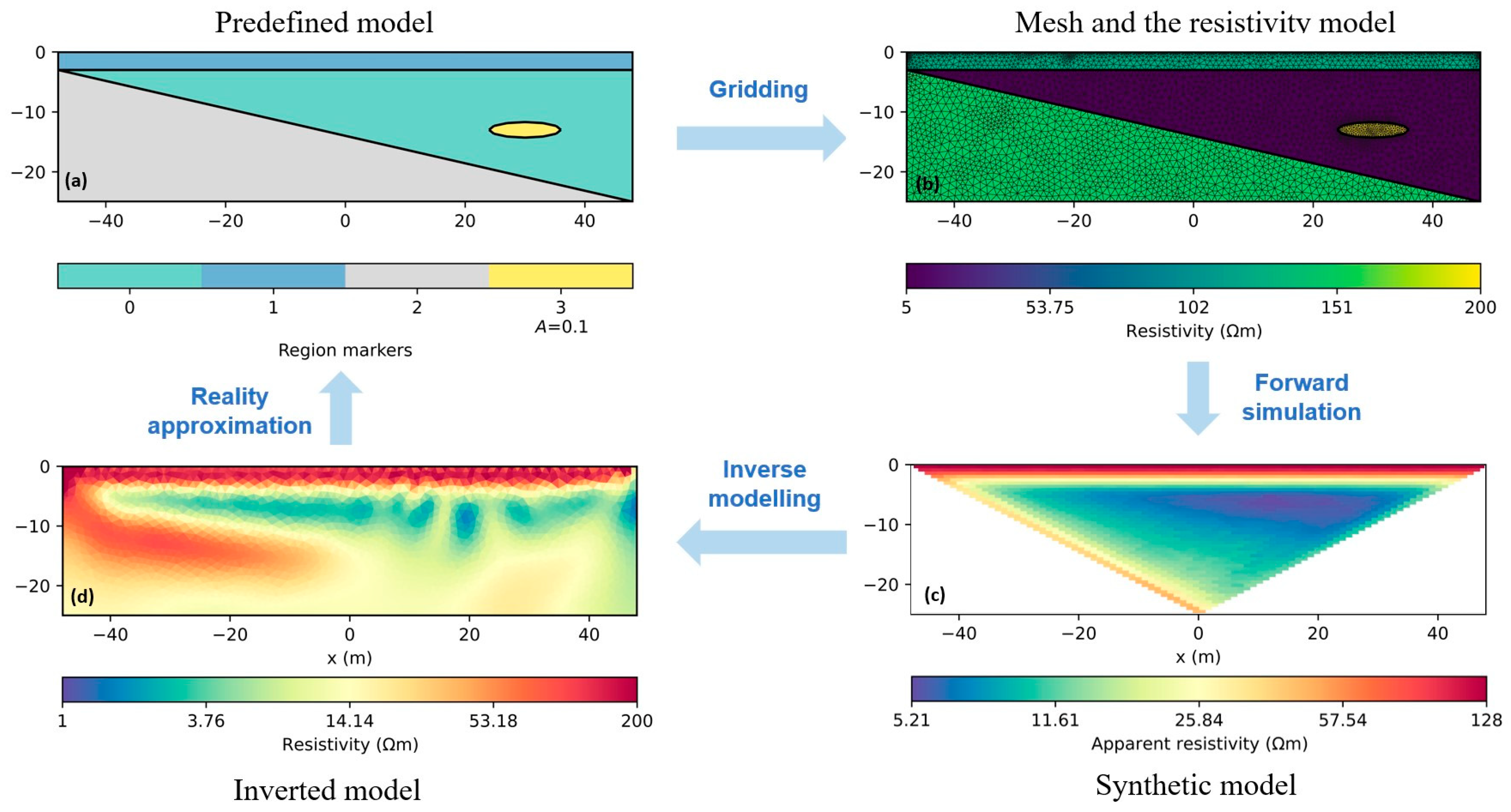
In Figure 1a, a predefined model with three region markers is illustrated. The gridding process involves creating a mesh specifically designed for finite element modeling, ensuring adequate quality and resolution for accurate simulations. The resulting pseudosection from the forward modeling is presented in Figure 1d, showcasing the apparent resistivity pseudosection, which resembles the outcomes from multi-electrode measurements, as seen in Figure 1c.

2.2.2. ERT Synthetic Model 2: Landslide

The second example (Figure 2) is derived from the study of a landslide, potentially including a cavity within the conductive layer, which illustrates the flexibility of handling complex geometries [49,50]. This inversion will be processed using the same four array configurations for comparison, with a 2 m electrode spacing, extending 96 m in the x-direction and reaching a depth of 25 m in the z-direction. The upper subsurface layer has a thickness of 3 m, while the landslide layer represents the underlying half-space to the north, and the conductive layer is located further south. These configurations are based on a real-world study, reflecting the actual geophysical characteristics observed in the study area [13,28]. A fourth rounded geometry was included, attributed to the presence of a cavity in the conductive layer. Additionally, the resistivities of the layers were defined. To make them more representative, average resistivity values, measured five times at various locations in the study area, were assigned [13]. The upper subsurface layer, composed mainly of alluvial deposits, has a resistivity of 125 Ωm; the landslide layer made up of hard, compact conglomerates has a resistivity of 150 Ωm; the homogeneous conductive layer located further south has a resistivity of 5 Ωm; and the region attributed to the presence of a cavity filled with sediment has a resistivity of 200 Ωm.
A direct simulation was conducted on the generated mesh to obtain synthetic data. After the simulation, potential differences were increased by a 3% error, which is crucial to ensure the synthetic data realistically reflect the model. However, these synthetic data are not expected to be entirely accurate, as geological models are rarely perfect and serve as proxies for real data. The additional error simulates random noise commonly found in real-world measurements. To evaluate the depth effect and compare inversion results, four different electrode array configurations were used—dipole–dipole, Schlumberger, Wenner-Alpha, and Wenner-Beta—under both open-source software tools.

2.3. Inverse Modeling

Inverse modeling leverages synthetic data to reconstruct a subsurface resistivity distribution that closely matches the measured data. During this inversion process, a regularization parameter of LAMBDA = 5 was employed to optimize data fitting, effectively balancing model flexibility and stability. This moderate value enabled the inversion to capture key geological features while minimizing the impact of noise within the synthetic dataset. By implementing this controlled approach, the risk of overfitting was reduced, allowing the model to accurately reflect true subsurface conditions without unnecessary complexity. After five iterations, the inversion concluded satisfactorily when the data fit achieved an acceptable root mean squared (RMS) error.
The inversion of the two synthetic resistivity models was performed using four electrode configurations—dipole–dipole, Schlumberger, Wenner-Alpha, and Wenner-Beta (dd, slm, wa, wb)—employing both the PyGIMLi and BERT software packages (Table 2). The primary objective was to evaluate the effectiveness of each configuration and software in accurately reconstructing subsurface resistivity under varying conditions. Initially, the inversions were conducted without any added noise, providing an idealized benchmark. Subsequently, synthetic noise levels of 2% and 3% were incorporated to simulate real-world measurement uncertainties.

3. Results and Discussion

3.1. Synthetic Model 1 Inversion Results

3.1.1. BERT M1 Inversion Results

The various inverted models and their corresponding misfit images (model responses) are presented in Figure 3. This figure shows the inversion results obtained using different electrode configurations (dd, wa, wb, slm) in terms of inversion models (left) and the 2D distribution of the misfit parameter (right). The models are plotted only for the first 25 m, as there are no anomalies in the original model below this depth, and all tested configurations accurately depict the subsurface resistivity. The RMS values and chi-squared (χ2) values for each configuration are provided in Table 3, allowing for a quantitative assessment of the model performance.
Due to the pixel size in the inversion, all models represent the two cavities as anomalies with geometries at least twice the size of the synthetic model. All electrode configurations successfully identify both the matrix layer and the two anomalies, but differences are evident in the pseudosections of the inverted models. The primary distinctions lie in the geometry, size, and depth of the cavities.
For the dipole–dipole configuration, the data achieved a root mean square (RMS) error of approximately 1.11%, with a Chi-squared (χ2) fit of 0.84, indicating a good adjustment. This configuration aligns well with the synthetic resistivity values, capturing the higher resistivity of the right cavity and the lower resistivity of the left one, though a ghost anomaly appears to the right of the conductive cavity, resembling a second, more resistive cavity.
In the case of the Wenner-Alpha configuration, the RMS error was around 0.94%, with a Chi-squared fit value of 0.87. This configuration does not identify the two cavities as effectively as the dipole–dipole setup, with the left conductive cavity showing higher resistivity values and larger geometry, while the right resistive cavity exhibits lower resistivity and a non-circular shape. This could lead to confusion with other ghost anomalies within the pseudosection, as highlighted by [50], who noted that data density in Wenner configurations is crucial for resolution capability.
The Wenner-Beta configuration yielded an RMS error of approximately 0.77% and a Chi-squared fit value of 0.59. It behaved qualitatively similarly to the Wenner-Alpha configuration but provided poorer assessments of resistivity and geometry. The conductive cavity was noted with low resistivity, although its geometric shape did not resemble a circle. Additionally, a ghost anomaly appeared at the same depth as the two cavities, potentially misinterpreted as another resistive structure.
Finally, for the Schlumberger configuration, the RMS error was about 0.90%, with a Chi-squared fit value of 0.80. This configuration excelled in accurately representing the geometry of both cavities and the resistivity distribution across the model. While it demonstrated good image resolution similar to the dipole–dipole configuration, some distortions were noted at the edges of the cavities, and no highly resistive ghost anomalies were present in the overall model.
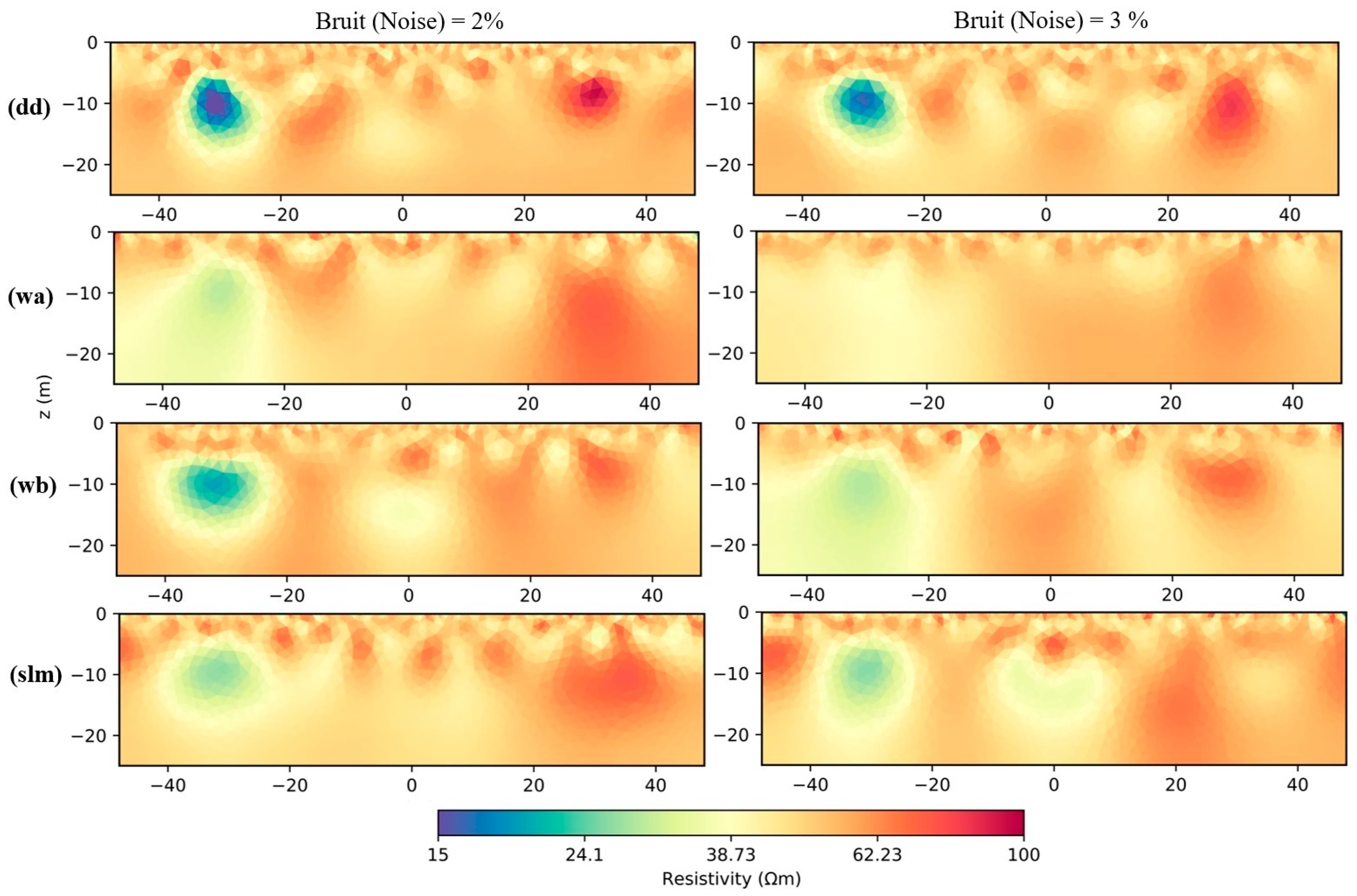
The corresponding results obtained with added noise for the same synthetic model data are presented in Figure 4, with 2% noise added on the left and 3% on the right. Both inversions were applied to study the behavior of resolution, data density, and sensitivity to different levels of added noise (2% and 3%). The introduction of noise leads to similar effects across all configurations: a decrease in the resistivity of the anomaly corresponding to the two cavities with differing resistivity values, and an increased offset in the resistivity of the two layers. Additionally, the dipole–dipole (dd) array produces numerous and more evident phantom anomalies, and the shape of the two cavities becomes less defined. Both Wenner-Alpha (wa) and Wenner-Beta (wb) arrays display a higher degree of smoothing as the noise level increases, complicating the interpretation of the results. The Schlumberger (slm) array also shows anomalies unrelated to the structures in the synthetic model, but they are significantly less intense compared to those in the dipole–dipole array.

3.1.2. PyGIMLi M1 Inversion Results

The inversion results using the PyGIMLi tool are illustrated in Figure 5, along with their model responses for each pseudosection. The RMS values and Chi-squared (χ2) values for each model are provided in Table 3, offering a quantitative evaluation of the inversion performance. The dipole–dipole electrode configuration (dd), inverted using PyGIMLi, shows data with a good fit, having an RMS error of about 1.19% and a chi-square fit below 1 (χ2 = 0.9), indicating a good match. The inversion result for the (dd) configuration aligns well with the synthetic model’s resistivity across the present formations. The rounded geometry and depth of both cavities are well represented, particularly for the conductive cavity, which exhibits an almost perfect shape and size match with the predefined synthetic model. However, the pseudosection shows several small phantom anomalies in the subsurface, though the boundary of the formations remains clearly identifiable.
For the Wenner-Alpha (wa) configuration inverted using PyGIMLi, the fit is slightly better, with an RMS error of 0.86% and a χ2 of 0.74, indicating an excellent fit. However, the (wa) configuration struggles to accurately identify both cavities. The conductive cavity on the left appears much larger than in the original model and has low resistivity values, although these are higher than those observed with the (dd) configuration. The resistive cavity on the right is barely highlighted, and its small size could be confused with other phantom anomalies at the center of the pseudosection.
The Wenner-Beta (wb) configuration shows a strong fit, with an RMS error of 0.66% and a χ2 of 0.44, indicating a near-perfect match. While it identifies both cavities well in terms of shape (mostly circular), their sizes are not consistent with the initial model. A phantom anomaly to the right of the conductive cavity appears at the same depth as the two cavities, which could be misinterpreted as a third cavity, conflicting with the original synthetic model.
Lastly, the Schlumberger (slm) configuration inverted by PyGIMLi achieves an RMS error of 0.96% and a near-perfect χ2 of 0.93. Contrary to the results from BERT, PyGIMLi produces a poorer resolution for the geometry and resistivity of the two cavities. The resistivity values for the conductive cavity are accurate, but its shape and depth are overestimated. The resistive cavity is marked by high resistivity values, but its geometry deviates significantly from the initial model. Furthermore, several phantom anomalies are present near the surface, although both cavities remain clearly recognizable.
Figure 6 presents the inversion results from simulations on the two buried cavities with the addition of random Gaussian noise (2% on the left and 3% on the right). In the (dd) configuration, the noise has a minimal effect, and both cavities remain clearly distinguishable, especially the conductive cavity, which retains the same geometry and depth as the initial model. Both (wa) and (wb) configurations exhibit a higher level of smoothing as the noise increases, making result interpretation more challenging. However, the (wb) configuration still highlights both cavities, though their geometry and depth deviate from the original model. In contrast, the (wa) configuration fails to provide visibility for the resistive cavity, and the conductive cavity is represented by a large anomaly, inaccurately reflecting the resistivity and geometry of the initial model. Unlike the (slm) configuration, which shows minor anomalies not related to the synthetic model structures but with much lower intensity than in the (wb) configuration, the conductive cavity is somewhat defined, though both geometry and depth are inaccurately represented. The resistive cavity, however, is barely visible due to the high level of smoothing and noise.

3.2. Synthetic Model 2 Inversion Results

3.2.1. BERT M2 Inversion Results

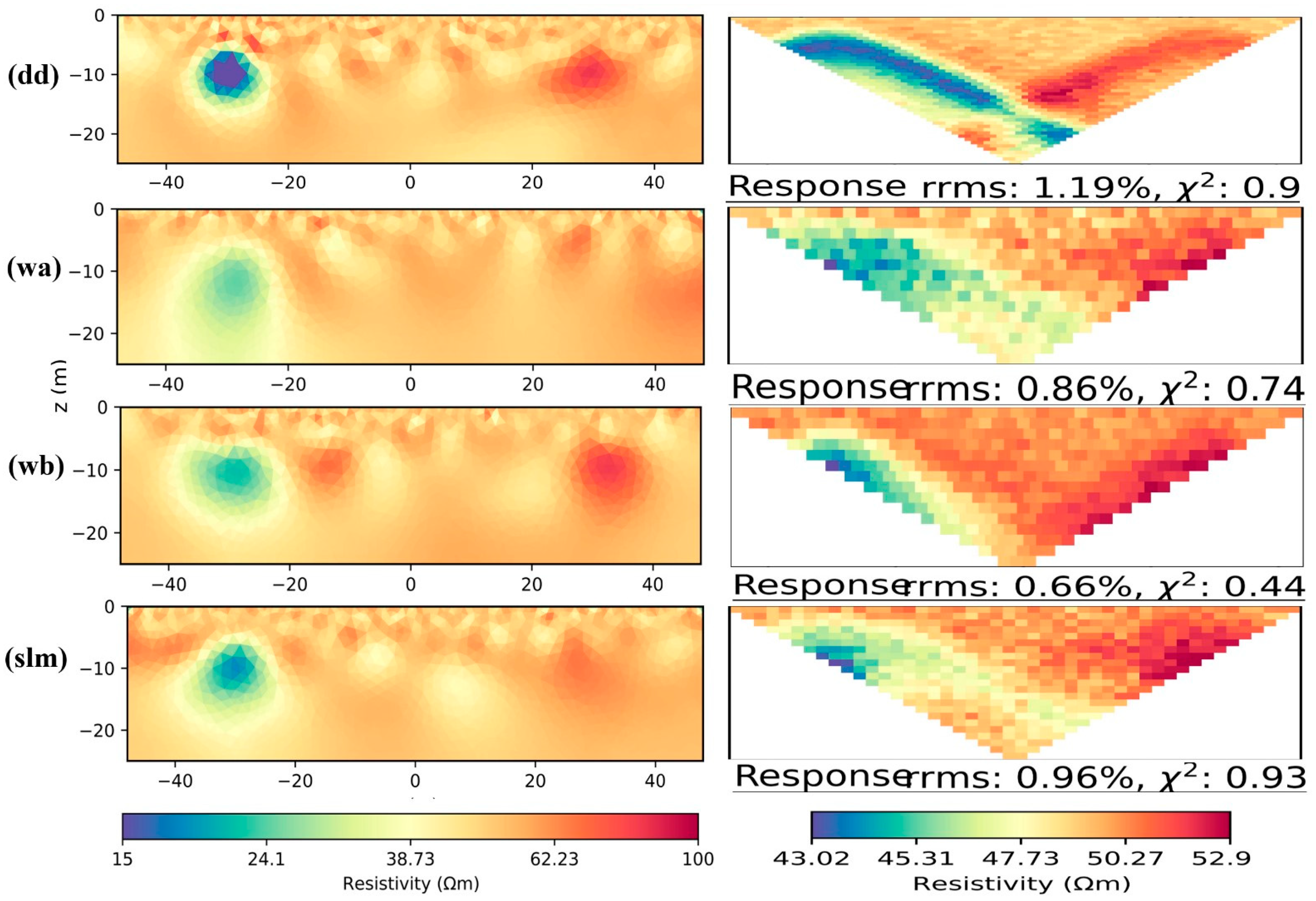
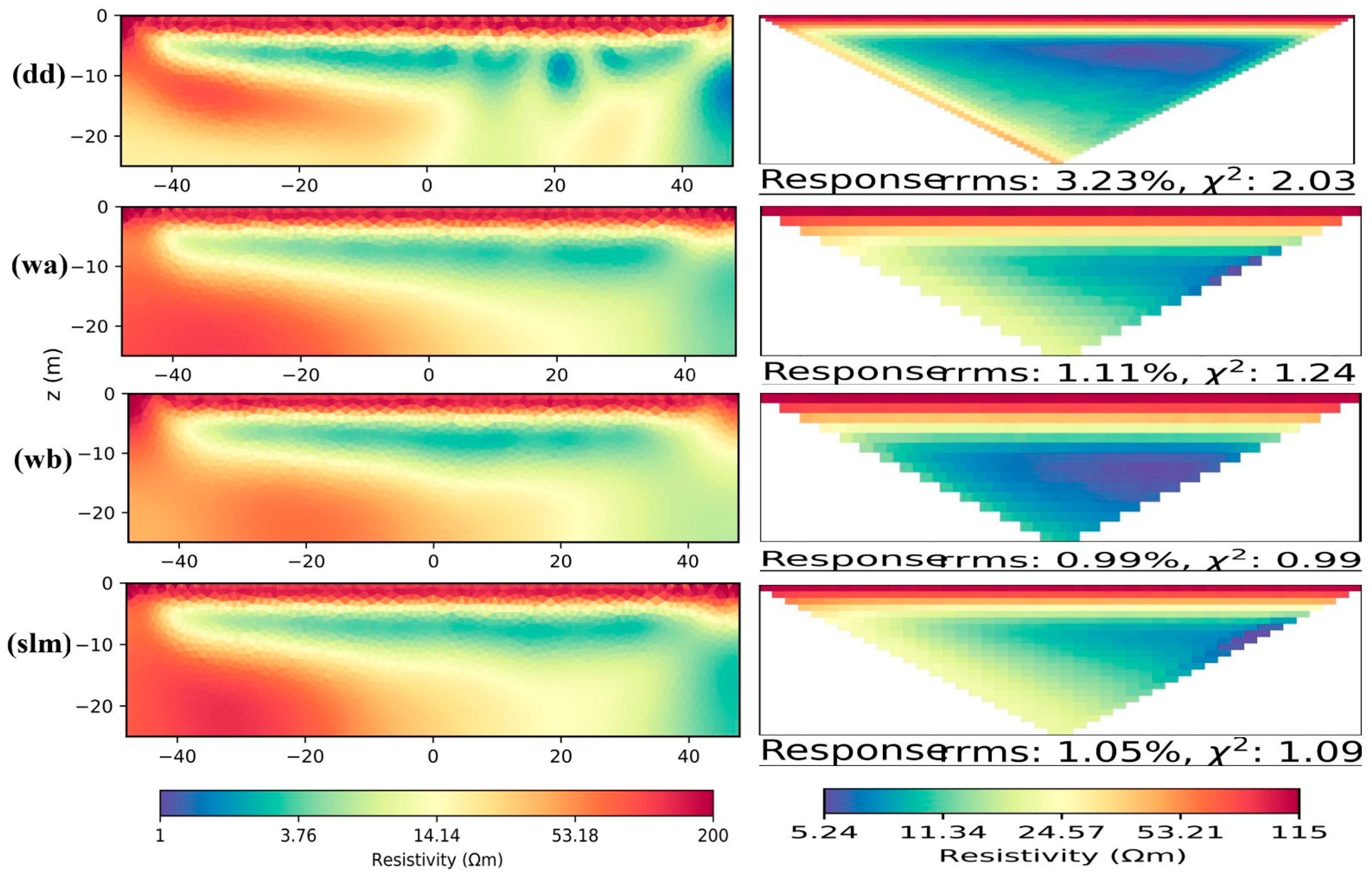
The various inverted models and their corresponding misfit images (model responses) for the landslide model are presented in Figure 7. This figure illustrates the inversion results obtained using different electrode configurations (dd, wa, wb, slm) in terms of inversion models (left) and the 2D distribution of the misfit parameter (right). The models are plotted only for the first 25 m, as there are no anomalies in the original model below this depth, and all configurations accurately depict the landslide form. The RMS values and Chi-squared (χ2) values for each configuration are provided in Table 4, allowing for a quantitative assessment of the model performance.
Figure 7 shows that for the dipole–dipole (dd) electrode configuration of the landslide model, the data are fitted with an acceptable relative root mean square error (rRMSE) of around 3.23% and a Chi-square value close to 1 (χ2 = 2.03), indicating a good fit. The (dd) configuration aligns better with the resistivity of the synthetic model of the different formations. The surface layer is resistive, accurately representing the distribution and depth of this formation, and the second sliding layer clearly shows the sliding angle and shape consistent with the initial model. However, a more resistive anomaly is noticeable, buried in the conductive matrix on the right (corresponding to the cavity in the same position in the synthetic model), and the (dd) configuration manages to show this anomaly independently of the more resistive layer on the left.
For the Wenner-Alpha (wa) configuration, the data are fitted with an rRMSE of around 1.11% and a Chi-square value close to 1 (χ2 = 1.24), indicating a near-perfect fit. The (wa) configuration does not identify the cavity as well as the (dd) configuration; lateral sensitivity is clearly less focused, suggesting a poorer definition of the elongated cavity buried within the conductor on the right of the pseudosection. The sensitivity decreases more rapidly with depth, which is beneficial for defining layer interface depths. However, the boundaries, geometry, and depth of the formations are well-respected compared to the initial model, particularly the sliding shape, which is more compact with stable resistivity values at depth.
For the Wenner-Beta (wb) configuration, the data are fitted with an rRMSE of around 0.99% and a Chi-square value below 1 (χ2 = 0.99), indicating a near-perfect fit. The (wb) configuration respects the synthetic model for the subsurface layer, sliding shape, and conductive formation, all with almost the same geometry and depth as the initial model. However, the inversion result using the (wb) configuration overestimates the depth of the underground layer on the right end of the pseudosection. The presence of the cavity is unclear due to an underestimation of resistivity within the conductive zone, as the boundary between the sliding mass and the anomaly attributed to the cavity is not well-defined in this configuration.
For the Schlumberger (slm) configuration, the data are fitted with an rRMSE of around 1.05% and a Chi-square value close to 1 (χ2 = 1.09), indicating a good fit. The (slm) configuration overestimates the depth of the subsurface layer on the right end of the pseudosection, just above the elongated cavity, which is also underestimated by lower resistivity values within the conductive formation. The boundary merges with the sliding mass, indicated by a rounded shape at the far-right end, which is inconsistent with the initial model. However, the boundaries, geometry, and depth of the formations are well-respected compared to the initial model, especially the sliding shape, which is more compact with stable resistivity values at depth.
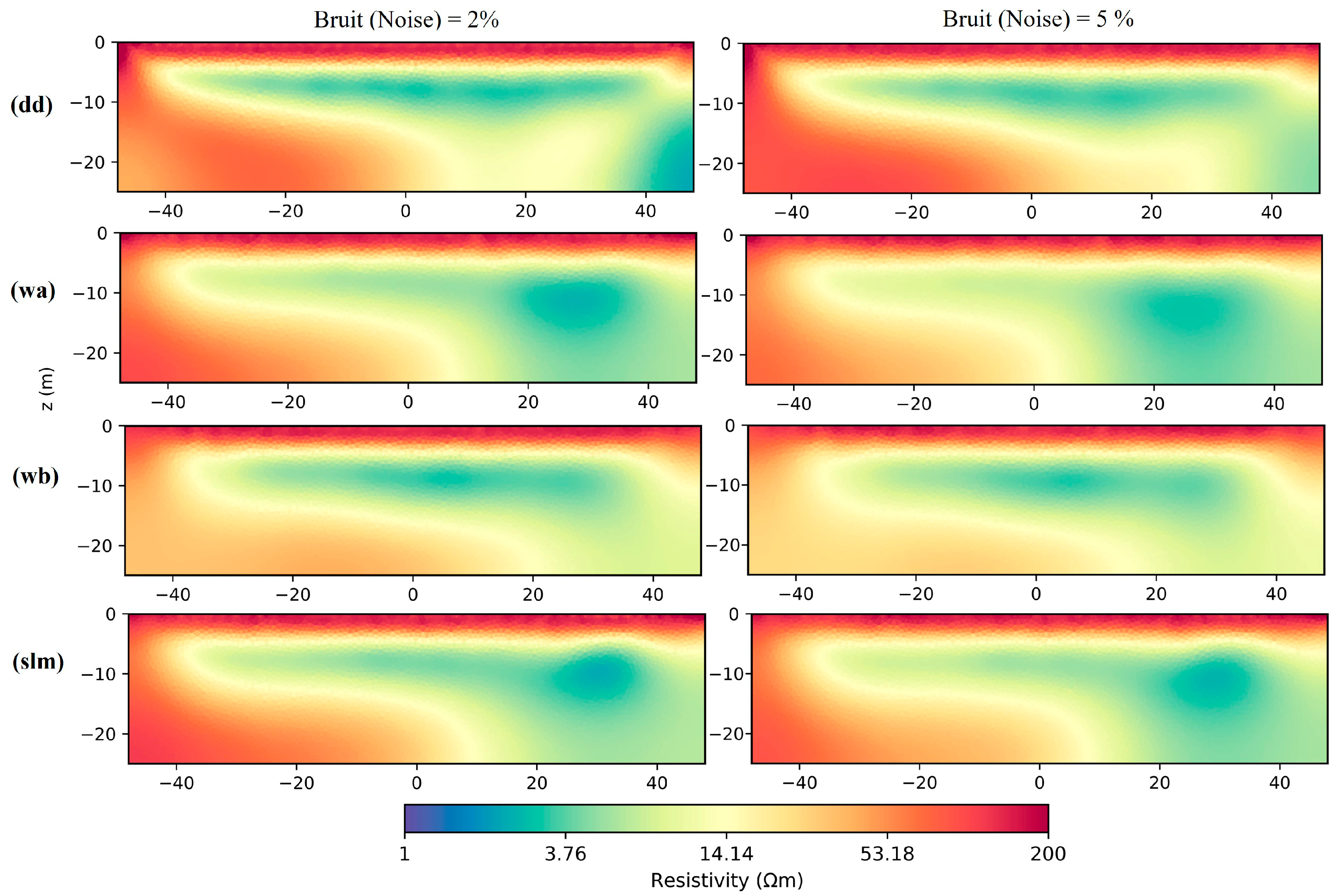
Figure 8 illustrates the inversions obtained from simulations on the initial landslide model, incorporating random Gaussian noise (2% on the left and 5% on the right). In all configuration models, the noise has a minimal effect on the subsurface formation and the landslide. Indeed, the characteristics of the inversions (obtained from all tested networks) remain similar to simulations using noise-free data for both formations, regardless of the noise level. This is likely due to the larger lateral dimensions of the structures being studied. The (dd) model consistently appears to be the configuration that best recognizes the structures of this model; the 2% noise level does not significantly disrupt the detection of the structures, while an increase in noise to 5% introduces some smoothing between the landslide mass and the cavity, making it difficult to distinguish the boundary between them.

3.2.2. PyGIMLi M2 Inversion Results

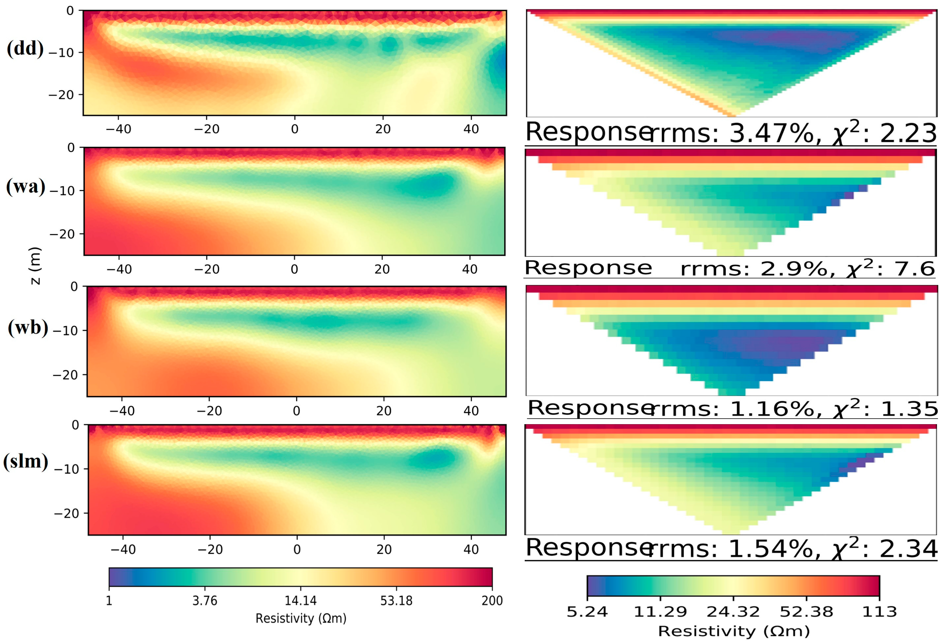
Figure 9 shows that the models were plotted only for the first 25 m, as there are no anomalies in the original model below this depth, and all tested electrode configurations accurately describe the subsurface resistivity. Due to the size of the inversion pixels, all inverted models present the landslide as a sliding mass with a geometry close to the synthetic model. However, the cavity is not represented as an anomaly in any of the resulting profiles. All electrode configurations successfully identify both the matrix layer and the sliding layer, but there are noticeable differences between the pseudosections of the inverted models. The main distinctions lie in the geometry, size, and underestimation of the cavity anomaly.
The (dd) configuration inverted by PyGIMLi for the landslide model shows well-fitted data, with a good rRMSE of about 3.47% and a Chi-squared adjustment close to 1 (χ2 = 2.23), indicating a good fit. The (dd) configuration resulting from the inversion by PyGIMLi aligns well with the resistivity of the synthetic model of the various formations. The surface layer is resistive in terms of distribution and depth, while the second sliding layer displays the angle and shape of the landslide as predicted by the initial model. However, a more resistive anomaly can be seen embedded in the conductive matrix on the right (this corresponds to the cavity at the same location in the synthetic model). Indeed, the shape of the anomaly is overestimated compared to the initial model; the (dd) configuration manages to show this anomaly as a cavity independent of the other formations and resistivities, successfully depicting this anomaly regardless of the more resistive layer on the left.
For the (wa) electrode configuration, the data are adjusted with an rRMSE of about 2.9% and a Chi-squared adjustment of 7.6, indicating a moderate fit. The (wa) network effectively delineates the boundaries of the formations, and their geometry and depth correspond well to the initial model, particularly the surface layer, which is resistive in terms of distribution and depth, and the shape of the landslide, which is clearly visible and more compact with stable resistivity values at depth. However, at greater depths, the contrasts are somewhat weaker, making it harder to highlight the presence of the cavity anomaly, which the (wa) network does not identify as well as the (dd) network. It is evident that the lateral sensitivity is less focused, suggesting a poorer definition of the characteristics of the elongated cavity submerged within the conductor on the right of the pseudosection, although this conductive matrix is well defined as per the initial model, with low resistivity and density at depth.
For the (wb) configuration inverted by PyGIMLi, the data are fitted, with an rRMSE of about 1.16% and a Chi-squared adjustment close to 1 (χ2 = 1.35), indicating a good fit. The (wb) network overestimates the depth of the subsurface layer at the far right of the pseudosection, just above the elongated cavity, which is also underestimated by lower resistivity values within the conductive formation. However, the (wb) network better identifies the cavity than the (wa) network in terms of resistivity values and geometry, although a clear boundary between the anomaly and the sliding shape cannot be identified. The lower resistivities may indicate the presence of an independent shape. The (wb) configuration manages to depict a resistive surface formation and the shape of the landslide as defined by the initial model, with these high resistivity values.
For the (slm) electrode configuration, the data are fitted with an rRMSE of about 1.54% and a Chi-squared adjustment close to 1 (χ2 = 2.34), indicating a good fit. Similarly to the (wb) network, the (slm) network also overestimates the depth of the subsurface layer at the far right of the pseudosection, just above the elongated cavity, which is also underestimated by lower resistivity values within the conductive formation. However, this configuration provides a shape and geometry closer to the initial model, although this boundary merges with the sliding mass, explained by a rounded shape at the far right of this formation, which does not align with the initial model. Thus, it is difficult to highlight the boundary of each limit. The other two regions, particularly the resistive subsurface layer and the sliding shape, are well respected in the pseudosection in accordance with the initial model, with stable and high resistivity values at depth.
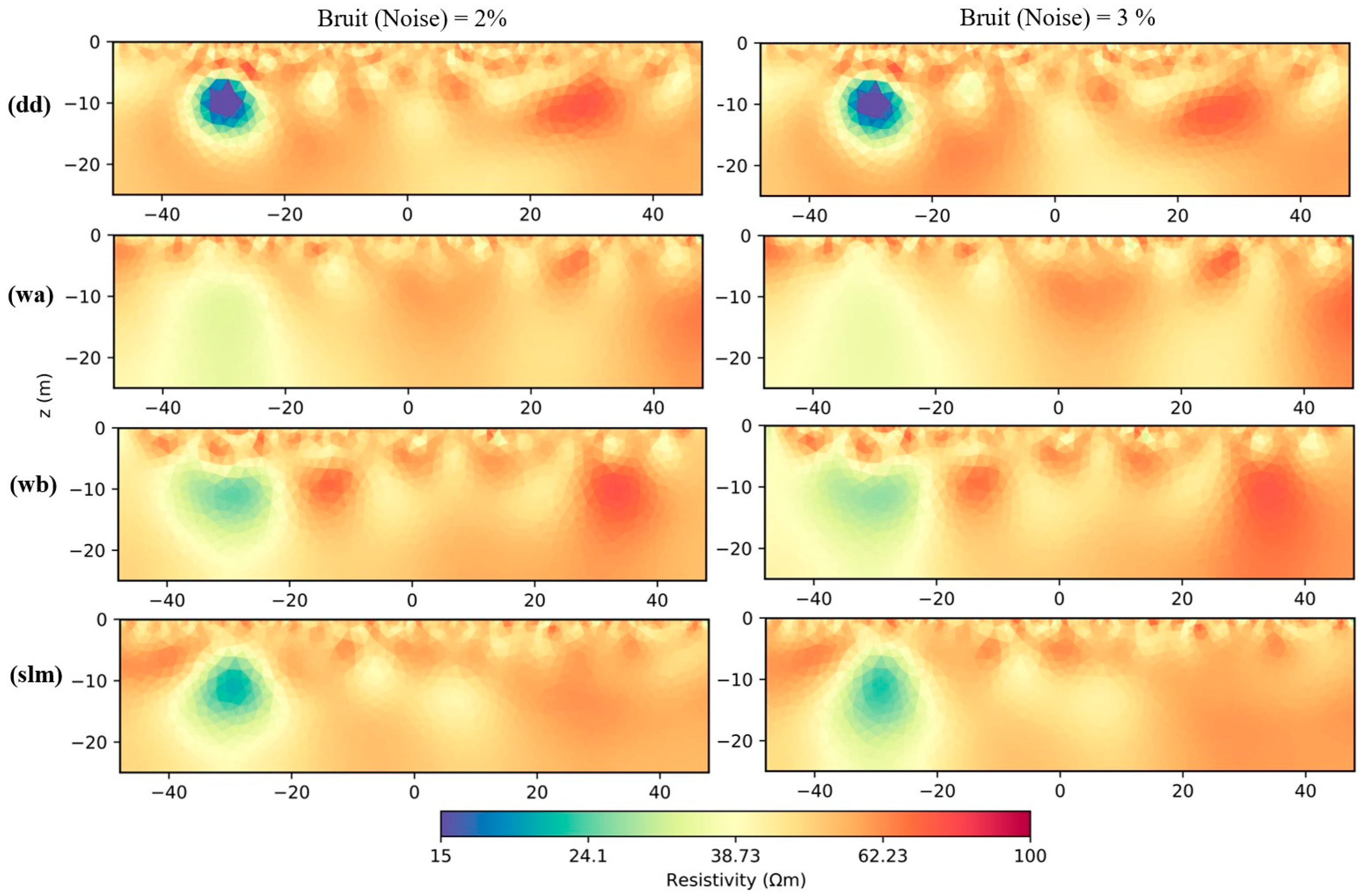
Figure 10 shows the inversions obtained from simulations on the initial landslide model using the PyGIMLi tool, with the addition of random Gaussian noise (2% on the left and 5% on the right). The noise has a minimal effect on the subsurface formation and the landslide across all configuration models. Indeed, regardless of the noise level, the characteristics of the inversions (obtained from all tested networks) remain similar to simulations based on noise-free data for these two formations. This is likely due to the larger lateral dimensions of the considered structures.
The (dd) model consistently appears as the configuration that best recognizes the predefined structures in the initial model; a noise level of 2% does not significantly disrupt the detection of the three structures, while increasing the noise to 5% leads to some smoothing between the sliding mass, which still shows its regular slope, and the anomaly attributed to the cavity, making it difficult to recognize the boundary between them.
The (wa) configuration shows a higher level of smoothing with increasing noise values; in both noisy profiles, the subsurface formation and the sliding mass appear resistive, while the conductive matrix forms a geometry that is more significant than that described by the initial model, complicating the interpretation of the cavity’s presence within this formation, especially with 2% noise, and making it nearly impossible at 5% noise. However, the (wb) configuration highlights the presence of the cavity with a resistive anomaly attached to the sliding shape due to smoothing, but it overestimates resistivity values at both edges of the 2% and 5% noise profiles. The subsurface formation presents regular higher resistivity values, identical to those of the initial model, and the sliding shape is well respected in geometry and form, even with lower resistivity values than all other configurations. In contrast, the (slm) configuration fails to display the high resistivity anomaly in both noise profiles (2% and 5%) within the conductive matrix, which is well respected in shape and size as described in the initial model, as well as the resistive subsurface area and the sliding mass. The (slm) configuration did not produce good inversion models when processed with PyGIMLi.

3.3. Limitations and Real-World Applicability of Synthetic Model

While this study provides valuable insights into the use of synthetic resistivity models, it is important to highlight the inherent limitations of these idealized models when translating the results to real-world applications. The models employed in this study, designed using both PyGIMLi and BERT inversion freeware, simulate subsurface conditions based on simplified geometries and resistivity values. However, actual geological environments are far more complex, with heterogeneity in material properties, structural features such as fractures or faults, and varying groundwater conditions. Consequently, the inversion results obtained from these synthetic models may not fully reflect the complexities encountered in natural subsurface environments. Inversion softwares like PyGIMLi and BERT, though powerful, also have their limitations in capturing these complexities. While PyGIMLi excels in flexibility, accommodating both structured and unstructured meshes for a wide variety of geophysical applications [34], BERT offers the advantage of a highly flexible mesh that can integrate complex topographies, though it may not perfectly simulate every geophysical anomaly in real-world settings [51].
In this study, the limitations of synthetic modeling also stem from the assumptions made about the geometry and depth of anomalies, which may not align with the variability of subsurface structures in field conditions. For example, the lack of geological noise, varying depths of anomalies, and more complex electrical conductivity contrasts in real scenarios may affect the accuracy and resolution of the models produced. Therefore, while the inversion results using PyGIMLi and BERT are promising, they should be validated further with real field data to assess their true applicability in geophysical surveys.
BERT and PyGIMLi share similarities in their code design and retrieval mechanisms, allowing for efficient forward and inverse modeling of geoelectrical data. One of the strengths of BERT is its highly flexible unstructured mesh, which can incorporate complex topographic features and subsurface structures [42,48]. PyGIMLi also utilizes both structured and unstructured meshes, implementing finite element and finite volume methods to enhance numerical accuracy. The unstructured mesh approach in both software packages refines grid sizes near electrode locations and target zones with high resistivity contrasts while enlarging them toward computational boundaries to maintain numerical stability [43,52].
Moreover, the numerical resistivity variations between PyGIMLi and BERT have been examined for different grid sizes, revealing slight discrepancies, particularly for small grid sizes. The impact of the anomaly effect—referring to variations in forward resistivity dataset accuracy—has been shown to be relatively consistent between PyGIMLi and BERT [9]. However, variations occur between different electrode arrays and geological conditions. This is particularly evident in the inversion resolution of small-scale targets, where PyGIMLi and BERT demonstrate superior performance compared to other freeware packages in previous studies [30,53,54].
The resolution of inverted models also varies depending on target size and survey depth. PyGIMLi and BERT effectively resolve subsurface features with a target diameter larger than one-fourth of its depth [30]. However, resolution significantly decreases for targets with a small radius at depths greater than 5 m, especially when the resistivity contrast is minimal or when the target’s resistivity closely approximates that of the surrounding formation. Furthermore, the smoothing effect in their inversion algorithms can lead to overestimation of conductive targets and underestimation of resistive targets at greater depths, emphasizing the need for field validation [55].
Future work should explore the potential of these inversion tools in more heterogeneous settings and consider the impact of real-world noise and measurement errors that often occur in field campaigns. Moreover, validating these models with actual geological data, particularly from regions with complex subsurface structures, will provide a more comprehensive understanding of the limitations and capabilities of PyGIMLi and BERT in practical geophysical investigations.

4. Conclusions

This study evaluated the effectiveness of PyGIMLi and BERT for geoelectric data inversion using synthetic models that simulate real subsurface conditions. By testing various electrode configurations, we assessed their impact on inversion accuracy and spatial resolution, particularly in detecting cavities and landslide-related features.
Results demonstrate that both software packages successfully reconstructed resistivity models under ideal conditions, but their performance varied in the presence of noise. In the cavity model, the dipole–dipole (dd) and Wenner-Alpha (wa) arrays provided the best spatial resolution, with BERT achieving higher inversion accuracy. However, under noisy conditions, only the dd configuration consistently yielded reliable results, highlighting its robustness in handling measurement uncertainties. PyGIMLi showed stable performance across configurations, with dd and Wenner-Beta (wb) excelling in detecting smaller features.
For the landslide model, both software packages effectively captured the general shape of the landslide, though smaller cavity features remained challenging to resolve. The dd array was the most effective in identifying the cavity, even in the presence of noise, underscoring its reliability in detecting subtle subsurface anomalies.
These findings emphasize the importance of selecting appropriate electrode configurations to enhance geophysical imaging accuracy. The study also reinforces the value of open-source geophysical software in advancing subsurface modeling and hazard detection. Further research should explore additional array configurations and noise effects in diverse geological settings to improve geoelectric data inversion techniques for real-world applications.

Author Contributions

Conceptualization, O.J. and P.M.-P.; methodology, O.J. and P.M.-P.; software, O.J. and P.M.-P.; validation, M.A.M.-S. and M.C.; formal analysis, O.J., P.M.-P. and X.C.-C.; investigation, O.J., P.M.-P. and K.D.; resources, O.J. and P.M.-P.; data curation, X.C.-C. and K.D.; writing—original draft preparation, O.J. and P.M.-P.; writing—review and editing, O.J. and P.M.-P.; visualization, O.J.; supervision, P.M.-P. and M.A.M.-S.; project administration, P.M.-P., M.C. and M.A.M.-S.; funding acquisition, P.M.-P. All authors have read and agreed to the published version of the manuscript.

Funding

This research received no external funding.

Data Availability Statement

The code and data used in this study are available at the following permanent repository link: https://github.com/Kingoussama94/geosciences-3369106 (accessed on 8 March 2025).

Acknowledgments

We sincerely appreciate the anonymous reviewer for their time and effort in providing insightful feedback that significantly contributed to enhancing the quality of our manuscript. Their constructive comments and thoughtful suggestions were invaluable in refining the content and ensuring that the final version met the highest standards. We acknowledge the importance of their contributions in improving the clarity, accuracy, and overall impact of our work.

Conflicts of Interest

The authors declare no conflicts of interest.

References

  1. Rey, J.; Mendoza, R.; Vilchez, J.; Hidalgo, M.C.; Fernández, I.; Berman, S. A Multidisciplinary Geophysical Approach to Characterize a Fracture Zone: The Southern Limit of the Mining District of Linares-La Carolina, Spain. Geosciences 2024, 14, 228. [Google Scholar] [CrossRef]
  2. Rupesh, R.; Tiwari, P.; Sharma, S.P. Estimation of Geotechnical Parameters for Coal Exploration from Quasi-3D Electrical Resistivity Measurements. Minerals 2024, 14, 102. [Google Scholar] [CrossRef]
  3. Papadopoulos, A.; Apostolopoulos, G.; Kallioras, A. An Integrated Hydrogeophysical Approach for Unsaturated Zone Monitoring Using Time Domain Reflectometry, Electrical Resistivity Tomography and Ground Penetrating Radar. Water 2024, 16, 2559. [Google Scholar] [CrossRef]
  4. Mendoza Trujillo, B.G.; Cadena Rojas, L.S.; Cisneros Barahona, A.S. Identification of the Hydrogeological Potential in Langos-San Andres, by Means of Electrical Resistivity Tomography Interpretation. Eng. Proc. 2023, 57, 44. [Google Scholar] [CrossRef]
  5. Hussain, Y.; Uagoda, R.; Borges, W.; Nunes, J.; Hamza, O.; Condori, C.; Aslam, K.; Dou, J.; Cárdenas-Soto, M. The Potential Use of Geophysical Methods to Identify Cavities, Sinkholes and Pathways for Water Infiltration. Water 2020, 12, 2289. [Google Scholar] [CrossRef]
  6. Jabrane, O.; Martínez-Pagán, P.; Martínez-Segura, M.A.; Alcalá, F.J.; El Azzab, D.; Vásconez-Maza, M.D.; Charroud, M. Integration of Electrical Resistivity Tomography and Seismic Refraction Tomography to Investigate Subsiding Sinkholes in Karst Areas. Water 2023, 15, 2192. [Google Scholar] [CrossRef]
  7. Lech, M.; Skutnik, Z.; Bajda, M.; Markowska-Lech, K. Applications of Electrical Resistivity Surveys in Solving Selected Geotechnical and Environmental Problems. Appl. Sci. 2020, 10, 2263. [Google Scholar] [CrossRef]
  8. Alam, M.J.B.; Ahmed, A.; Alam, M.Z. Application of Electrical Resistivity Tomography in Geotechnical and Geoenvironmental Engineering Aspect. Geotechnics 2024, 4, 399–414. [Google Scholar] [CrossRef]
  9. Dahlin, T.; Zhou, B. A numerical comparison of 2D resistivity imaging with 10 electrode arrays. Geophys. Prospect. 2004, 52, 379–398. [Google Scholar] [CrossRef]
  10. Sharma, S.; Verma, G.K. Inversion of Electrical Resistivity Data: A Review. Int. J. Comput. Syst. Eng. 2015, 9, 400–406. [Google Scholar]
  11. Romano, G.; Capozzoli, L.; Abate, N.; De Girolamo, M.; Liso, I.S.; Patella, D.; Parise, M. An Integrated Geophysical and Unmanned Aerial Systems Surveys for Multi-Sensory, Multi-Scale and Multi-Resolution Cave Detection: The Gravaglione Site (Canale di Pirro Polje, Apulia). Remote Sens. 2023, 15, 3820. [Google Scholar] [CrossRef]
  12. Martinez-Lòpez, J.; Rey, J.; Duenas, J.; Hidalgo, C.; Benavente, J. Electrical tomography applied to the detection of subsurfacecavities. J. Cave Karst Stud. 2013, 75, 28–37. [Google Scholar] [CrossRef]
  13. Jabrane, O.; El Azzab, D.; Martínez-Pagán, P.; Charroud, M.; El Mansouri, B.; Martínez-Segura, M.A.; Himi, M.; Elgettafi, M. Comparison of the PyGIMLi and BERT packages for Landslide and Cavity Detection: A Case Study from Tghat-Oued Fez, Morocco. J. Earth Syst. Sci. 2023, 132, 107. [Google Scholar] [CrossRef]
  14. Telford, W.M.; Geldart, L.P.; Sheriff, R.E.; Keys, D.A. Applied Geophysics; This book covers various methods, including ERT configurations; Cambridge University Press: Cambridge, UK, 1990. [Google Scholar]
  15. Szalai, S.; Szarka, L. On the classification of surface geo-electric arrays. Geophys. Prospect. 2008, 56, 159–175. [Google Scholar] [CrossRef]
  16. Wilkinson, P.B.; Meldrum, P.I.; Kuras, O.; Chambers, J.E.; Holyoake, S.J.; Ogilvy, R.D. High-Resolution Electrical Resistivity Tomography Monitoring of a Tracer Test in a Confined Aquifer. J. Appl. Geophys. 2010, 70, 268–276. [Google Scholar] [CrossRef]
  17. Loke, M.H. Tutorial: 2-D and 3-D Electrical Imaging Surveys. Geotomo Software, Res2dinv 3.5 Software. 2004. Available online: https://www.researchgate.net/publication/264739285_Tutorial_2-D_and_3-D_Electrical_Imaging_Surveys (accessed on 12 January 2025).
  18. Jabrane, O.; Azzab, D.E.; Himi, M.; Charroud, M.; Gettafi, M.E. Detection of Underground Cavities Using Electromagnetic GPR Method in Bhalil City (Morocco). In Proceedings of the International Conference on Digital Technologies and Applications, Fes, Morocco, 28–30 January 2021; pp. 1111–1120. [Google Scholar]
  19. Storz, H.; Storz, W.; Jacobs, F. Electrical Resistivity Tomography to Investigate Geological Structures of the Earth’s Upper Crust. Geophys. Prospect. 2000, 48, 455–471. [Google Scholar] [CrossRef]
  20. Martorana, R.; Capizzi, P.; D’Alessandro, A.; Luzio, D. Comparison of different sets of array configurations for multichannel 2D ERT acquisition. J. Appl. Geophys. 2017, 137, 34–48. [Google Scholar] [CrossRef]
  21. Cubbage, B.; Noonan, G.E.; Rucker, D.F. A Modified Wenner Array for Efficient Use of Eight-Channel Resistivity Meters. Pure Appl. Geophys. 2017, 174, 2705–2718. [Google Scholar] [CrossRef]
  22. AL-Hameedawi, M.M.; Thabit, J.M. Comparison between four electrode arrays in delineating sedimentary layers of alluvial fan deposits in eastern Iraq using a 2D imaging technique. Environ. Earth Sci. 2017, 76, 525. [Google Scholar] [CrossRef]
  23. Abdullah, F.M.; Loke, M.; Nawawi, M.; Abdullah, K. Assessing the reliability and performance of optimized and conventional resistivity arrays for shallow subsurface investigations. J. Appl. Geophys. 2018, 155, 237–245. [Google Scholar]
  24. Martorana, R.; Capizzi, P. Evaluation of Artifacts and Misinterpretation in 2D Electrical Resistivity Tomography Caused by Three-Dimensional Resistive Structures of Regular or Irregular Shapes. Appl. Sci. 2023, 13, 2015. [Google Scholar] [CrossRef]
  25. Doyoro, Y.G.; Chang, P.-Y.; Puntu, J.M. Uncertainty of the 2D Resistivity Survey on the Subsurface Cavities. Appl. Sci. 2021, 11, 3143. [Google Scholar] [CrossRef]
  26. Dosoky, W. Assessment of three mixed arrays dataset for subsurface cavities detection using resistivity tomography as inferred from numerical modelling. SN Appl. Sci. 2023, 5, 303. [Google Scholar] [CrossRef]
  27. Quiceno-Arenas, B.A.; Paniagua-Castrillón, J.G.; Muñoz-García, A.M.; Duque-Gómez, L.F.; Bustamante-Rúa, M.O. Open-Source Learning as a Skill for Geoelectrical Data Processing: The Case of PyGIMLi. 2022. Available online: https://www.researchgate.net/publication/362263536 (accessed on 12 January 2025).
  28. Jabrane, O.; El Azzab, D.; Martínez-Pagán, P.; Martínez-Segura, M.A.; Mahjoub, H.; Charroud, M. Contribution of Python-based BERT software for landslide monitoring using Electrical Resistivity Tomography datasets. A case study in Tghat-Fez (Morocco). Data Brief 2022, 46, 108763. [Google Scholar] [CrossRef] [PubMed]
  29. Nickschick, T.; Flechsig, C.; Mrlina, J.; Oppermann, F.; Löbig, F.; Günther, T. Large-Scale Electrical Resistivity Tomography in the Cheb Basin (Eger Rift) at an International Continental Drilling Program (ICDP) Monitoring Site to Image Fluid-Related Structures. Solid Earth 2019, 10, 1951–1969. [Google Scholar] [CrossRef]
  30. Doyoro, Y.G.; Chang, P.-Y.; Puntu, J.M.; Lin, D.-J.; Van Huu, T.; Rahmalia, D.A.; Shie, M.-S. A review of open software resources in python for electrical resistivity modelling. Geosci. Lett. 2022, 9, 3. [Google Scholar] [CrossRef]
  31. Yang, X.; Lagmanson, M.B. Planning resistivity surveys using numerical simulations. In Proceedings of the Annual Symposium for the Application of Geophysics to Environmental and Engineering Problems, San Antonio, TX, USA, 6–10 April 2003; Environmental and Engineering Geophysical Society: Denver, CO, USA, 2003; pp. 488–501. [Google Scholar]
  32. Olayinka, A.; Yaramanci, U. Assessment of the reliability of 2D inversion of apparent resistivitydata. Geophys. Prospect. 2000, 48, 293–316. [Google Scholar]
  33. Dahlin, T.; Loke, M.H. Resolution of 2D Wenner resistivity imaging as assessed by numerical modelling. J. Appl. Geophy. 1998, 38, 237–249. [Google Scholar] [CrossRef]
  34. Rücker, C.; Günther, T.; Wagner, F.M. PyGIMLi: An open-source library for modelling and inversion in geophysics. Comput. Geosci. 2017, 109, 106–123. [Google Scholar] [CrossRef]
  35. Du, Q.; Wang, D.; Zhu, L. On mesh geometry and stiffness matrix conditioning for general finite element spaces. SIAM J. Numer. Anal. 2009, 47, 1421–1444. [Google Scholar] [CrossRef]
  36. Neumaier, A. Solving ill-conditioned and singular linear systems: A tuto-rial on regularization. J. Soc. Ind. Appl. Math. 1998, 40, 636–666. [Google Scholar] [CrossRef]
  37. Shewchuk, J.R. Triangle: Engineering a 2D Quality Mesh Generator and Delaunay Triangulator, Workshop on Applied Computational Geometry; Springer: Berlin/Heidelberg, Germany, 1996; pp. 203–222. [Google Scholar]
  38. Si, H. TetGen, a Delaunay-based quality tetrahedral mesh generator. ACM Trans. Math. Softw. 2015, 41, 11. [Google Scholar] [CrossRef]
  39. Geuzaine, C.; Remacle, J.F. Gmsh: A 3-D finite element mesh generator with built-in pre-and post-processing facilities. Int. J. Numer. Methods Eng. 2009, 79, 1309–1331. [Google Scholar] [CrossRef]
  40. Hunter, J.D. Matplotlib: A 2D graphics environment. Comput. Sci. Eng. 2007, 9, 90–95. [Google Scholar] [CrossRef]
  41. Ayachit, U. The Paraview Guide: A Parallel Visualization Application; Kitware Inc.: New York, NY, USA, 2015. [Google Scholar]
  42. Günther, T.; Rücker, C.; Spitzer, K. 3D Modeling and Inversion of DC Resistivity Data Incorporating Topography—Part II: Inversion. Geophys. J. Int. 2006, 166, 506–517. [Google Scholar]
  43. Rücker, C.; Günther, T.; Spitzer, K. Three-Dimensional Modelling and Inversion of DC Resistivity Data Incorporating Topography—Part I: Modelling. Geophys. J. Int. 2006, 166, 495–505. [Google Scholar] [CrossRef]
  44. Tarantola, A. Inverse Problem Theory and Methods for Model Parameter Estimation, 1st ed.; The Society for Industrial and Applied Mathematics (SIAM): Philadelphia, PA, USA; Cambridge University Press: Cambridge, UK, 2005; 352p. [Google Scholar]
  45. Mehanee, S. A new scheme for gravity data interpretation by a faulted 2-D horizontal thin block: Theory, numerical examples and real data investigation. IEEE Trans. Geosci. Remote Sens. 2022, 60, 1–14. [Google Scholar] [CrossRef]
  46. Rücker, C.; Günther, T. The simulation of finite ERT electrodes using the complete electrode model. Geophysics 2011, 76, F227–F238. [Google Scholar]
  47. Ronczka, M.; Rücker, C.; Günther, T. Numerical study of long-electrode electric resistivity tomography—Accuracy, sensitivity, and resolution. Geophysics 2015, 80, E317–E328. [Google Scholar] [CrossRef]
  48. Günther, T.; Rücker, C. Boundless Electrical Resistivity Tomography BERT2—The User Tutorial. 26 April 2023, Version 2.4.1. 2019. Available online: http://www.resistivity.net/download/bert-tutorial.pdf (accessed on 13 October 2024).
  49. Zhou, B.; Greenhalgh, S.A. Cross-Hole Resistivity Tomography Using Different Electrode Configurations. Geophys. Prospect. 2000, 48, 887–912. [Google Scholar] [CrossRef]
  50. Jabrane, O.; Martínez-Pagán, P.; El Azzab, D.; Martínez-Segura, M.A.; Urruela, A. A review of Python-based code for landslide modeling and inversion using Electrical Resistivity Tomography method. Simul. Model. Pract. Theory 2023, 111, 101501. [Google Scholar] [CrossRef]
  51. Audebert, M.; Clément, R.; Grossin-Debattista, J.; Günther, T.; Touze-Foltz, N.; Moreau, S. Influence of the geomembrane on time-lapse ERT measurements for leachate injection monitoring. J. Waste Manag. 2014, 34, 780–790. [Google Scholar] [CrossRef] [PubMed]
  52. Blanchy, G.; Saneiyan, S.; Boyd, J.; McLachlan, P.; Binley, A. ResIPy, an intuitive open source software for complex geoelectrical inversion/modeling. Comput. Geosci. 2020, 137, 104423. [Google Scholar] [CrossRef]
  53. Flechsig, C.; Fabig, T.; Rücker, C.; Schütze, C. Geoelectrical Investigations in the Cheb Basin/W-Bohemia: An Approach to Evaluate the Near-Surface Conductivity Structure. Stud. Geophys. Geod. 2010, 54, 443–463. [Google Scholar] [CrossRef]
  54. Jordi, C.; Doetsch, J.; Günther, T.; Schmelzbach, C.; Maurer, H.; Robertsson, J. Structural joint inversion on irregular meshes. Geophys. J. Int. 2020, 220, 1995–2008. [Google Scholar] [CrossRef]
  55. Portniaguine, O.; Zhdanov, M.S. Focusing Geophysical Inversion Images. Geophysics 1999, 64, 874–887. [Google Scholar] [CrossRef]
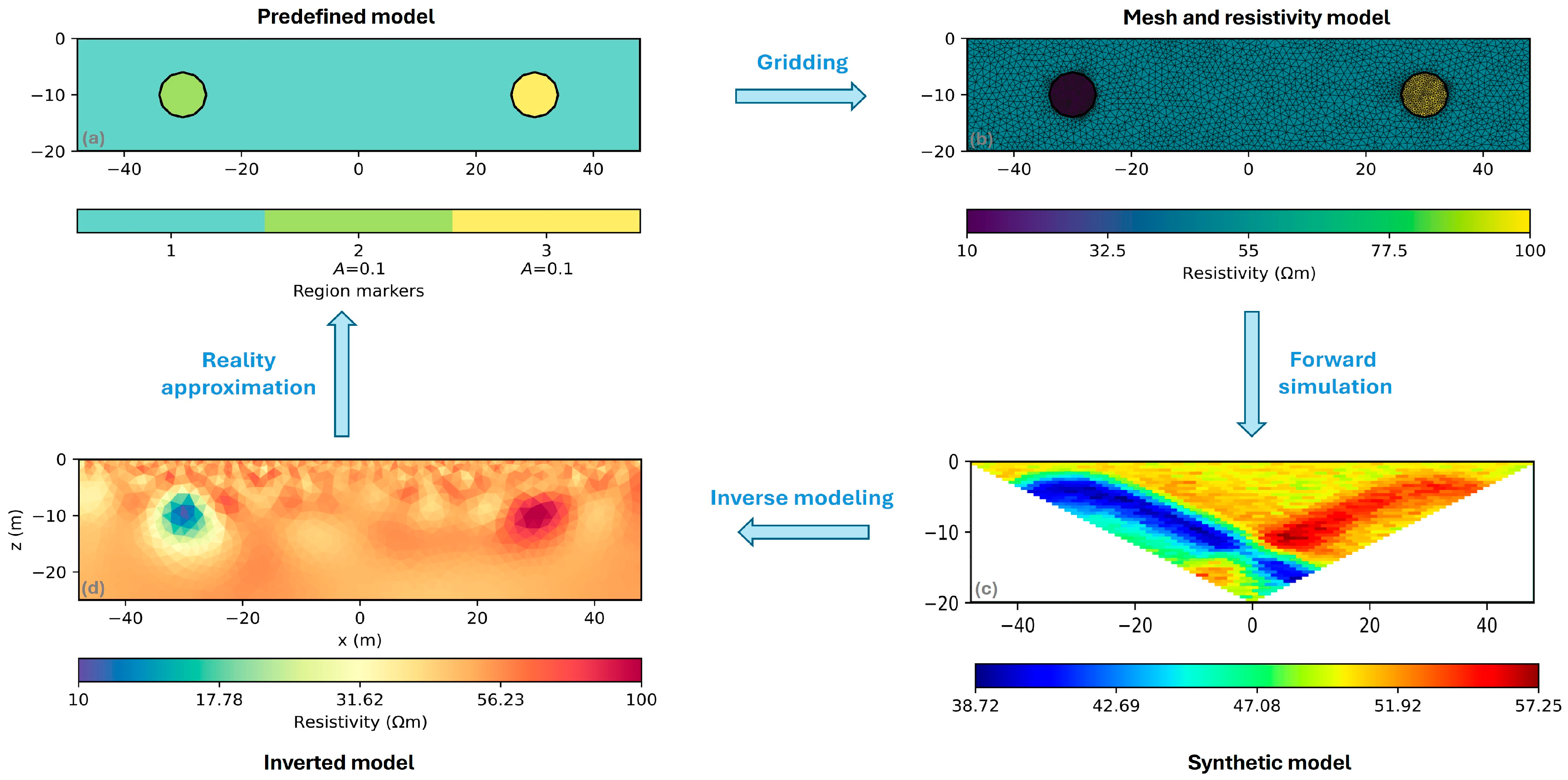
Figure 1. The fundamental structure of geoelectric forward-inverse modeling involves (a) a predefined model representing a homogeneous formation that contains two cavities of the same size and shape; (b) discretization of the model for numerical computation; (c) a synthetic model displaying the apparent resistivity data generated from the forward modeling; and (d) the inverted model result, which represents the response of the resistivity inversion process.
Geosciences 15 00127 g001
Figure 2. The core framework of geoelectric data forward-inverse modeling includes (a) a predefined conceptual model featuring a sloped structure and a small, rounded target body simulating a potential cavity, (b) discretization of the model into computational elements, (c) a synthetic dataset illustrating the apparent resistivity distribution, and (d) the resulting model response.
Geosciences 15 00127 g002
Figure 3. Inversion results for the various electrode configurations—dipole–dipole (dd), Wenner-Alpha (wa), Wenner-Beta (wb), and Schlumberger (slm)—along with their model responses after simulation using BERT (on the right) for the model of the two underground cavities.
Geosciences 15 00127 g003
Figure 4. Inversion results for the different electrode configurations—(dd) dipole–dipole, (wa) Wenner-Alpha, (wb) Wenner-Beta, and (slm) Schlumberger—using BERT, after adding noise (3% on the right and 2% on the left), for the model of two underground cavities.
Geosciences 15 00127 g004
Figure 5. Inversion results for the different electrode configurations—(dd) dipole–dipole, (wa) Wenner-Alpha, (wb) Wenner-Beta, (slm) Schlumberger—and their model responses (on the right) after simulation using PyGIMLi for the model of the two underground cavities.
Geosciences 15 00127 g005
Figure 6. Inversion results for different electrode configurations using PyGIMLi, including (dd) dipole–dipole, (wa) Wenner-Alpha, (wb) Wenner-Beta, and (slm) Schlumberger, after the addition of noise (3% on the right and 2% on the left), for the model of the two underground cavities.
Geosciences 15 00127 g006
Figure 7. Inversion results for the different electrode configurations—(dd) dipole–dipole, (wa) Wenner-Alpha, (wb) Wenner-Beta, (slm) Schlumberger—and their model responses after simulation (on the right) by BERT for the landslide model.
Geosciences 15 00127 g007
Figure 8. Inversion results for the different electrode configurations by BERT, including (dd) dipole–dipole, (wa) Wenner-Alpha, (wb) Wenner-Beta, and (slm) Schlumberger, after adding noise (5% on the right and 2% on the left), for the landslide model.
Geosciences 15 00127 g008
Figure 9. Inversion results for different electrode configurations—(dd) dipole–dipole, (wa) Wenner-Alpha, (wb) Wenner-Beta, and (slm) Schlumberger—along with their model responses after simulation (to the right) by PyGIMLi, for the landslide model.
Geosciences 15 00127 g009
Figure 10. Inversion results for different electrode configurations by PyGIMLi—(dd) dipole–dipole, (wa) Wenner-Alpha, (wb) Wenner-Beta, (slm) Schlumberger—after adding noise (5% on the right and 2% on the left), for the landslide model.
Geosciences 15 00127 g010
Table 1. Applications, scope, and limitations of DC resistivity for hazard detection in synthetic modeling.
ApplicationScopeLimitations
Cavity detectionSimulates the resistivity response of air- or water-filled voids to assess detectability.Depth penetration and resolution depend on the chosen array. Dipole–dipole enhances shallow cavity detection but loses sensitivity at depth. Wenner-Alpha and Beta improve lateral resolution, while Schlumberger provides better depth sensitivity but lower detail.
Landslide detectionModels’ resistivity variations to identify weak zones and potential failure planes.Sensitivity to landslide features varies with electrode configuration. Dipole–dipole captures near-surface instabilities, Wenner arrays highlight lateral changes, and Schlumberger is better for deeper slip surfaces but less effective in complex terrains.
Table 2. Inversion settings for synthetic models in PyGIMLi and BERT simulations.
ParameterValueDetails
Total Length96 mThe horizontal distance of the electrode array used in the survey, as indicated in the code (grange(start = −48, end = 48, n = 48)).
Mesh Quality33.5Mesh quality specified in the code during mesh creation: quality = 33.5. The mesh is generated with a target quality factor to ensure that the resulting mesh elements are geometrically suitable for inversion.
Maximum Depth25 mThe maximum investigation depth, set to 25 m in the code (paraDepth = 25). The inversion depth is limited to 25 m for all electrode configurations.
λ (Regularization)5Regularization parameters are used to control the smoothing of the inversion model. A higher value of λ leads to a smoother model. This value is provided in the inversion function (lam = 5).
Max Cell Size1 mThe maximum cell size is used in the inversion model. This is defined in the code (paraMaxCellSize = 1), which affects the spatial resolution of the model.
VerbosityTrueThe verbosity setting is enabled (verbose = True) to show detailed output during the inversion process.
Data Noise Level1The code specifies this as noiseLevel = 1, which adds Gaussian noise to the simulated data. The standard deviation mof the noise is proportional to the data values, ensuring a realistic representation of measurement uncertainty.
Data Noise Absolute1e-6The absolute noise level specified as noiseAbs = 1e-6, indicating the minimum possible noise added to the data.
Table 3. Comparison of model performance based on Chi-squared (χ2) and root mean square (RMS) values.
Chi-Squared (χ2)Root Mean Square (RMS)
BERT Cavity Modeldd = 0.84
wa = 0.87
wb = 0.59
slm = 0.8
dd = 1.11%
wa = 0.94%
wb = 0.77%
slm = 0.9%
PyGIMLi Cavity Modeldd = 0.9
wa = 0.74
wb = 0.44
slm = 0.93
dd = 1.19%
wa = 0.86%
wb = 0.66%
slm = 0.96%
Table 4. Comparison of the landslide model performance based on Chi-squared (χ2) and root mean square (RMS) values.
Chi-Squared (χ2)Root Mean Square (RMS)
BERT Landslide Modeldd = 2.03
wa = 1.24
wb = 0.99
slm = 1.09
dd = 3.23%
wa = 1.11%
wb = 0.99%
slm = 1.05%
PyGIMLi Landslide Modeldd = 2.23
wa = 7.6
wb = 1.35
slm = 2.34
dd = 3.47%
wa = 2.9%
wb = 1.16%
slm = 1.54%
Disclaimer/Publisher’s Note: The statements, opinions and data contained in all publications are solely those of the individual author(s) and contributor(s) and not of MDPI and/or the editor(s). MDPI and/or the editor(s) disclaim responsibility for any injury to people or property resulting from any ideas, methods, instructions or products referred to in the content.