Article

Micropolar Modeling of Shear Wave Dispersion in Marine Sediments and Deep Earth Materials: Deriving Scaling Laws

Institut de Physique du Globe de Paris, CNRS, Université de Paris, 75005 Paris, France
Geosciences 2025, 15(4), 124; https://doi.org/10.3390/geosciences15040124
Submission received: 27 December 2024 / Revised: 12 March 2025 / Accepted: 28 March 2025 / Published: 1 April 2025
(This article belongs to the Special Issue Seismology of the Dynamic Deep Earth)

Abstract

:
We draw connections between eight different theories used to describe microscopic (atomic) and macroscopic (seismological) scales. In particular, we show that all these different theories belong to a particular case of a single partial differential equation, allowing us to gain new physical insights and draw connection among them. With this general understanding, we apply the micropolar theory to the description of shear-wave dispersion in marine sediments, showing how we can reproduce observations by only using two micropolar parameters in contrast to the seventeen parameters required by modifications of Biot’s theory. We next establish direct connections between the micro (laboratory) and macro (seismological) scales, allowing us to predict (and confirm) the presence of post-perovskite in the lowermost mantle based on laboratory experiments and to predict the characteristic length L c at which shear deformation becomes significant at seismological scales in the lowermost mantle.

1. Introduction

Seismologists analyze seismic waveforms (e.g., amplitudes, polarities, frequency content, and travel times) in order to invert them for seismic velocities (and hopefully densities) and to obtain seismic tomographic images of the interior of the Earth. These images have shown through the decades that the Earth is highly heterogeneous at all scales ranging from meters to hundreds of kilometers [1,2,3,4,5,6,7,8].
In order to infer the materials that these seismic images are made up, seismologists closely collaborate with mineral scientists that perform experiments at extreme pressure/temperature conditions resembling those inside the Earth [9,10,11,12,13]. However, these experiments are performed over samples of the order of crystalline scales (see Figure 1). As a result, a bridge between spatial scales is needed in order to reconcile seismological and mineralogical results.
The methodology to extrapolate laboratory observations (microscales) to global Earth’s scales (macroscales) is not yet fully understood in seismology [14]. An important inconsistency observed between laboratory experiments and seismological observations can be exemplified with the hot creep (tendency of a solid material to deform permanently under the influence of hot mechanical stresses) experiments of olivine and olivine-bearing rocks, where results have shown that the strain rates appear to be significantly higher than those indicated by geophysical evidence [15].
Figure 1. From the microscale to the macroscale observations; from [16]. Colors of the crystal unit cell and the aggregate of atoms that represent the structure of bridgmanite silicate perovskite ( Mg , Fe ) SiO 3 : Red circles represent oxygen atoms, orange circles magnesium or iron atoms and green circles silicon atoms. The silicon atoms are located at the centre of the blue SiO 6 octahedrons. Colors of the granular media and the Earth represent different random materials.
Geosciences 15 00124 g001
Seismologists face a fundamental problem when comparing seismic velocities measured on samples of the size of a single crystal (see Figure 1) against velocities obtained from seismological observations/inversions (see Figure 1). To properly take into account every spatial scale, it is necessary to clearly understand the relationship between the micro- and macroscales. Homogenization techniques have been developed and enable to find the equivalent effective medium [17,18,19,20,21,22]. Similar averaging methods are also employed for finding the equivalent macroscale-averaged elastic parameters from laboratory experiments performed on microsamples [23]. These techniques are based on averaging methodologies that provide the equivalent macroscale medium. At mesoscale lengths, i.e., intermediate scales between seismological observations and laboratory experiments, statistical methods are often used [24,25].
Material scientists face a similar problem connecting micro- and macroscales in numerical simulations when modeling crystalline nano-structures [26,27,28,29]. At microscopic (atomic) scales, theories like quantum mechanics, lattice mechanics, molecular dynamics, and density functionals are used, while at macroscopic scales, the conventional theory of linear elasticity is used (see Figure 2). It thus becomes necessary to define a transition region between the two scales, where a certain coupling theory is defined. This coupling theory is not yet well defined and/or accepted and it does not have a unique answer yet either [30,31,32,33]. Often, Eringen’s theory of non-local continuum mechanics [34] is used (see Figure 2). However, even if the coupling theory is well defined, from a practical point of view, the problem is even more complicated, since the coupling leads to large numerical errors in the solutions [30,31,32,33].
Motivated by ideas of the material scientists’ community, we aim to couple micro- and macroscales for applications in seismology in a clear, theoretical, and transparent way using a recently introduced micropolar theory by [35]. To this end, we first find consensus on the understanding of what is commonly called a micro-continuum theory. We show how all these theories can be reconciled in a single equation, having direct and documented applications in different areas such as civil engineering (Timoshenko’s equation), solid-state physics (lattice theory), seismic metamaterials (materials with frequency band gaps), granular materials (micropolar model), and biological materials (microstretch model).
After the theoretical clarifications/developments, we show how we can model shear-wave dispersion in marine sediments using the micropolar theory with gradient micro-inertia. This allows us to use only two parameters to reproduce observations in contrast to the seventeen parameters required by modifications of Biot’s theory. We next propose a simple way to connect laboratory scales with seismological observations (see Figure 1). This allows us to predict the characteristic length L c at which shear deformation becomes significant at seismological scales in the lowermost mantle. Finally, we discuss the implications of our findings related to the Earth’s internal structure and draw conclusions from this work.

2. Theoretical Developments: Drawing Connections Between Micro, Macro and Mass-in-Mass Theories

The common conceptual use of linear continuum mechanics is the description of macroscopic objects without attempting to describe the microstructure [36]. In order to describe the physical phenomena in studies when the material deviates from the linear elastic behavior, different terms are added to the equation of motion such as in the case of viscoelasticity, non-linearities, plasticity, etc. [37,38]. Still, however, all this is conducted without attempting to properly describe the microstructure of the material.
At atomic scales, the picture is different; scientists try to describe the fundamental microstructure and atomic interactions of the material. There are numerous ways to do this by, for example, applying theories like quantum mechanics, lattice mechanics, and the density functional theory [39,40,41].
A more recent view is to use/develop models based on continuum mechanics that attempt to include the microstructure [34,37,42,43,44,45,46]. The main idea of these models is to include in the (continuum) equations of motion, the degrees of freedom generated by the microstructure. The spatial scales that these models apply vary from atomic [47,48,49,50,51], mesoscales [52,53,54,55,56] to macroscopic scales [42,57,58,59,60,61,62,63]. In this work, we refer to all these models as micro-continuum models. They all can be understood as a continuum homogenization [64].
To develop physical intuition, we show in Figure 3a the common interpretation of the linear elastic model. In general, the linear elastic model is related to small deformations, i.e., the curvature induced by the deformations are very smooth. On the other hand, micro-continuum models describe larger deformations, i.e., deformations that produce larger curvatures that are understood/interpreted as the new degrees of freedom(s) (see Figure 3b).
We next draw (not-obvious) connections between continuum (macroscales), micro-continuum (micro- or macroscales) and lattice (microscales) theories.

2.1. The General (Continuum) Equation

To draw connections between continuum, micro-continuum, and lattice theories, i.e., atomic (laboratory) scales and macroscopic (Earth) scales, we show that all these models belong to a single partial differential equation (PDE). This has important consequences since it means that, depending on the parameter selection, they show the same frequency-dispersion behavior and, as a consequence, describe the same phenomena.
The general PDE that all these models belong to is given by the following expression
t 4 c x t 2 t 2 x 2 + c x 4 4 x 4 + ω r 2 ( t 2 c x 2 2 x 2 ) ( var 1 , var 2 ) = 0 ,
where we have used two colors to separate partial derivative terms (red color) from their parameters (blue color). The variables ( var 1 , var 2 ) refer to two different variables that, depending on the parameter selection, describe the wave motion.
Looking at Equation (1), we can identify the following five partial derivative terms:
t 2 —acceleration.
t 2 x 2 —rotatory inertia [65].
x 4 —Euler–Bernoulli term (from beam theory [66]). It accounts for the bending stiffness.
t 4 —Timoshenko term [67].
x 2 —spatial curvature.
To simplify the notation for the terms accompanying each partial derivative, we use c for velocity and ω for (angular) frequency. The sub-indexes of each term are given by the partial derivative terms that they multiply, like, for instance, the sub-index x t multiplies the term t 2 x 2 , the sub-index x 2 multiplies the term x 2 , etc. We thus have the following four terms
c x t 
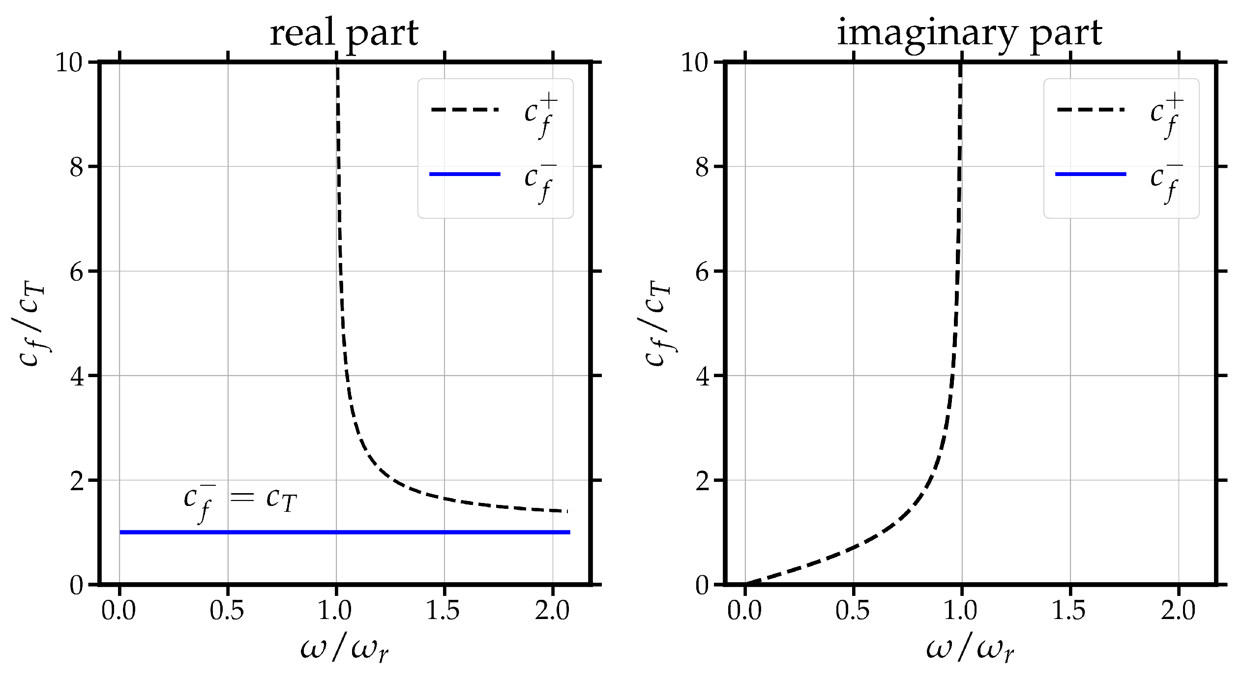
is the limit of phase (and group) (rotatory) velocity at high frequencies.
c x 4 is the limit of phase (and group) velocity at high frequencies.
ω r 
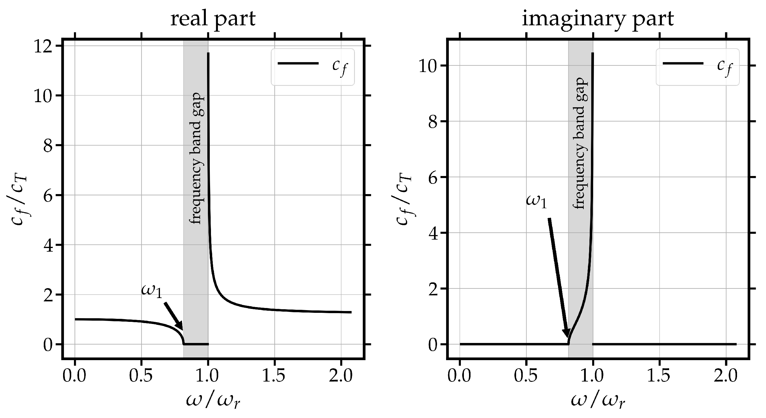
is the resonant (cut-off) frequency (optic mode). No real signal propagates at that frequency.
c x 2 is the limit of phase (and group) velocity at low frequencies.
If we assume plane-wave propagation of the form
var 1 ( x , t ) , var 2 ( x , t ) = A 1 , A 2 e i ( k x + ω t ) ,
where A = [ A 1 , A 2 ] are the (unknown) amplitudes, k the wavenumber, and ω the angular frequency, we can write Equation (1) as follows:
A · γ ¯ = 0 .
In order to obtain non-trivial solutions ( A 0 ) of Equation (3), one must impose that
det γ ¯ = 0 .
Equation (4) is called the dispersion relation and we can use it to obtain explicit expressions for the frequency ω as a function of the wavenumber k, or the other way around, and/or for the phase velocity ω / k as a function of frequency. In this work, we are interested in finding expressions for the phase velocity ω / k for each theoretical model using Equation (4).
If we assume wave propagation in the form of Equation (2) and substituting into general Equation (1), we can find an expression for the phase velocity given by
ω 2 k 2 = c x 2 2 ω r 2 ω 2 c x t 2 ± c x 2 2 ω r 2 ω 2 c x t 2 2 4 1 ω r 2 ω 2 c x 4 4 2 1 ω r 2 ω 2 ,
which leads to the two limiting cases
lim ω ω 2 k 2 = c x t 2 ± c x t 4 4 c x 4 4 2 , and lim ω 0 ω 2 k 2 = c x 2 2 .
Thus, we name the terms c x 2 as the limit of phase (and group) velocity at low frequencies and c x 4 and c x t as the limits of phase (and group) velocities at high frequencies.
In our analyses, we keep the comparisons limited to 1D, since the conclusions can be directly extrapolated to general 3D scenarios. We next explore the lattice and continuum description of linear elasticity and how to find connections among them.

2.2. The Macroscopic Description: Linear Continuum Mechanics

Accepted more than a century ago [68], the theory that describes earthquake motions, away from the rupture zone, is the theory of linear continuum mechanics [36,69,70]. We next show how in 1D, the equations of motion for P and S waves can be obtained from lattice descriptions [51].

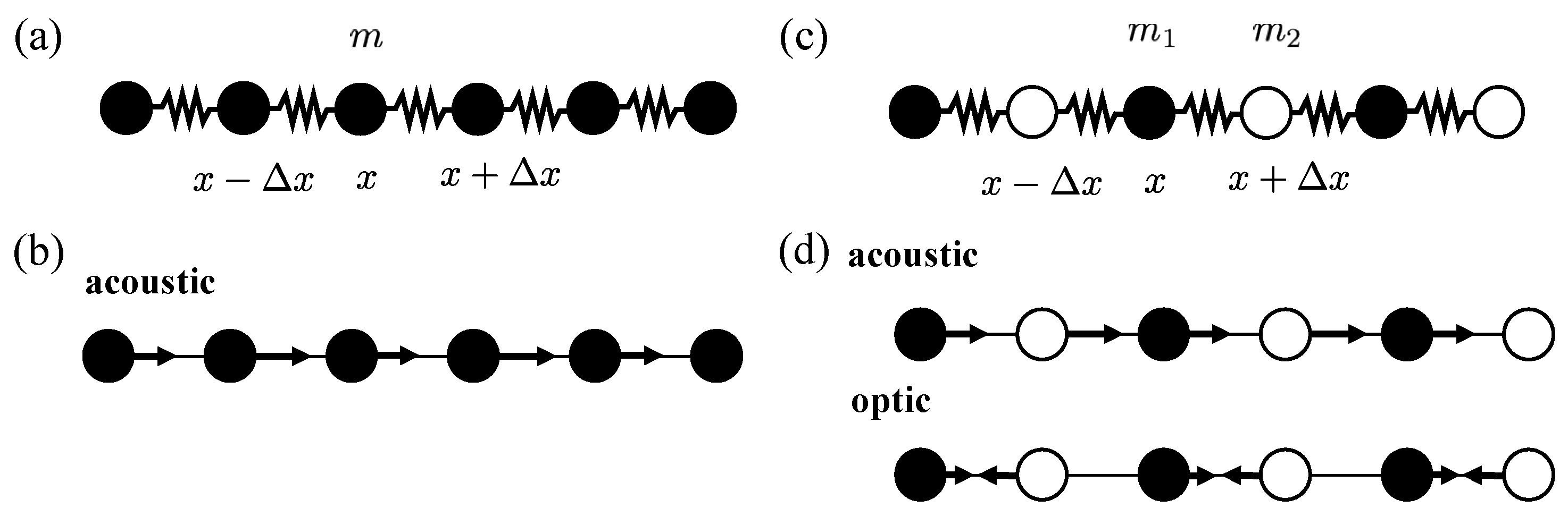
2.2.1. Linear Elasticity: Lattice Description

Consider the mono-atomic chain given in Figure 4a. All atoms (black circles) are connected by a (linear) spring with constant C and separated by a distance Δ x . The spring constant C is physically interpreted as the interatomic force (elastic) constant.
If we consider two nearest neighbors to the location x, the total (effective) force ( F ) exerted on the xth atom in the lattice is given by the following expression
F = C ( u x + Δ x u x ) C ( u x u x Δ x ) ,
from which Newton’s second law yields the lattice equation of motion given by
m t 2 u x = C u x + Δ x 2 u x + u x Δ x ,
where m is the mass of the atom. A similar equation to Equation (8) can be written for each atom in the lattice. This results in a system of N coupled differential equations (where N is the total number of atoms in the lattice) which describe the acoustic modes of the lattice (see Figure 4b) [39].

2.2.2. Linear Elasticity: Continuum Description

Acoustic and/or elastic 1D descriptions of wave propagation (in homogeneous media) can be summarized in the following second-order PDE
t 2 u = c 2 x 2 u ,
where c 2 refers to the wave propagation velocity, e.g., for S waves, we have c 2 = μ / ρ , for P waves, c 2 = ( λ + 2 μ ) / ρ , where the parameters λ , μ are the classical Lamé parameters and ρ the material density [36]. Assuming plane-wave propagation in the form
u ( x , t ) = A e i ( k x + ω t ) ,
where A is the amplitude, k the wavenumber, and ω the angular frequency, and substituting Equation (10) into the equation of motion, Equation (9), assuming c 2 = μ / ρ , we can write the following expression for the (squared) phase velocity ( ω / k ) :
ω 2 k 2 = μ ρ ,
where we can observe that the phase velocity is linear. This correspond to the (constant) acoustic mode given in Figure 4a. Note that the wave equation given in Equation (9) is a particular case of the general equation, Equation (1), where c x 4 = c x t = t 4 = 0 .

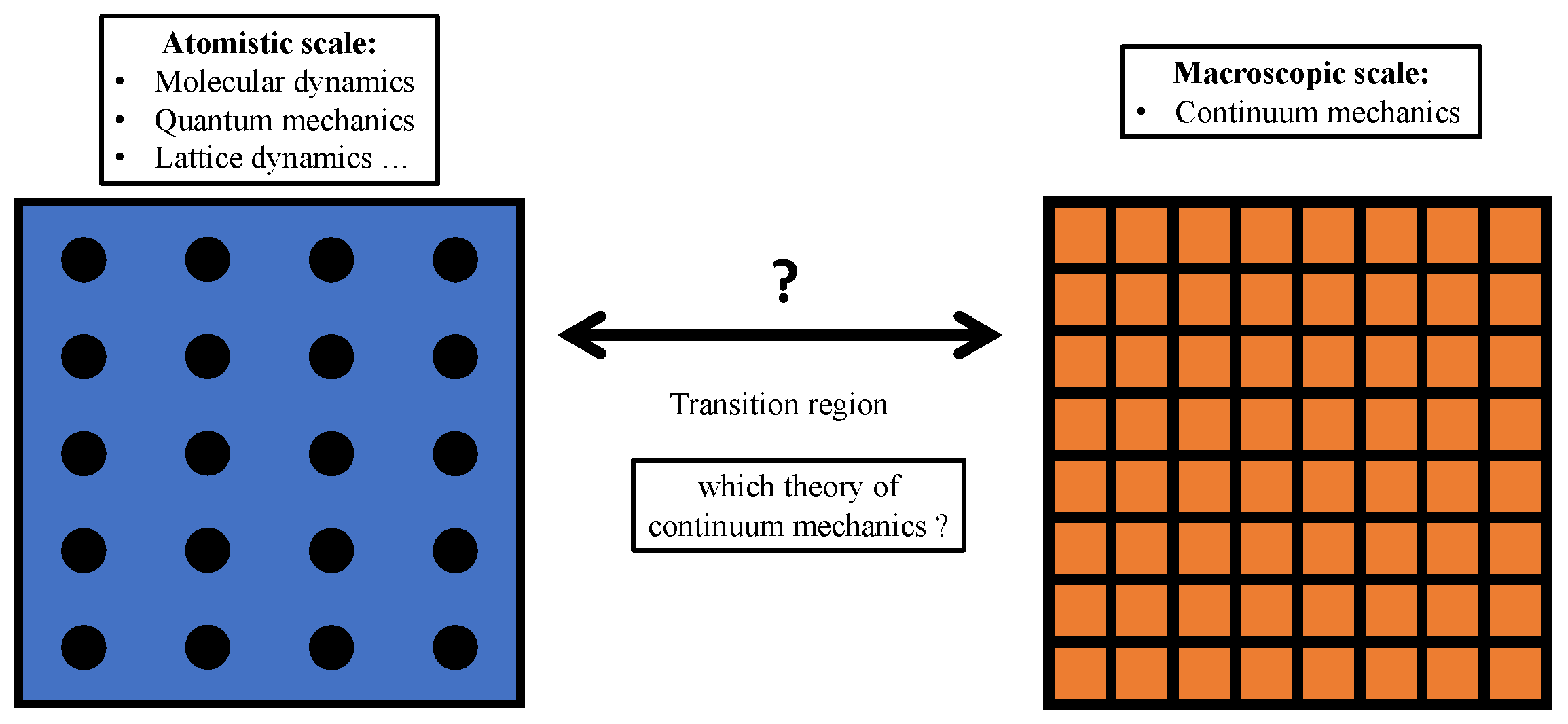
2.2.3. How Do We Pass from the Lattice to the Continuum Description?

The simplest way to convert lattice into continuum equations (of motion) is by using Taylor’s series approximation. Let us take for instance Equations (8) and (9). If we divide lattice Equation (8) by the volume V of the atom and call u = u x and C / V = μ / Δ x 2 , where μ is the shear modulus, we can write it as follows:
ρ t 2 u x t = μ u x + Δ x t 2 u x t + u x Δ x t Δ x 2 ,
where ρ = M / V is the material density. The expression inside the brackets is Taylor’s series (second-order approximation) of the second derivative [71]. This mean that we can write Equation (12) as follows:
ρ t 2 u μ x 2 u + O ( Δ x 2 ) ,
where the term O ( Δ x 2 ) refers to the Taylor’s series’s (second-order) error made in the approximation. Note that if we remove the error term in Equation (13), and call c 2 = μ / ρ , then Equations (9) and (13) are equivalent. For the physical interpretation, we refer to Figure 4a, where we can observe that Δ x is the spacing between atoms.
As a general criterion, we need a lattice of five atoms (four Δ x ’s) to build a continuum description out of a lattice description [72]. This means that the minimum wavelength that the continuum description can apply is four times the minimum wavelength of the lattice ( Δ x ) , i.e, 4 Δ x .

2.3. The Microscopic Descriptions: Lattice and/or Continuum?

When we attempt to find the dynamic equations of motion that correctly describe a complex lattice and/or continuum, we need to take into account the microstructure, i.e., the additional degrees of freedom that are required to properly describe the medium. As a consequence, microscopic descriptions may not be unique and depend on the problem at hand. We next present a lattice/continuum description commonly used in solid-state physics.

2.3.1. The Lattice Model of Two Atoms per Primitive Unit Cell

Elastic vibration of a crystal with two atoms per unit cell (or diatomic unit cell), for instance NaCl and diamond, can be described by means of lattice dynamics showing a unique frequency/wavenumber behavior [39]. A lattice model for the diatomic unit cell is presented in Figure 4c, where the model shows two different atoms alternately connected and separated by a distance Δ x . The mathematical model that describes the elastic deformation of the lattice is given by the following equations [39]
m 1 t 2 u x = C v x + v x Δ x 2 u x , m 2 t 2 v x = C ( u x + u x + Δ x 2 v x ) ,
where m 1 , m 2 are the masses of each atom, C is the force constant between the atoms separated by a distance Δ x , and u , v refers to the acoustic and optic modes, respectively (Figure 4d).
We can obtain a continuum approximation of the model given in Equation (14) by dividing by the volume and replacing first- and second-order derivatives by their finite-difference (Taylor’s series) approximations [51], as follows:
v x + v x Δ x 2 u x = ( v x + v x Δ x + v x + Δ x 3 v x ) + 3 v x v x + Δ x 2 u x = ( v x + Δ x 2 v x + v x Δ x ) ( v x + Δ x v x ) + 2 ( v x u x ) = Δ x 2 x 2 v Δ x x v + 2 ( v x u x ) + O ( Δ x ) , u x + u x + Δ x 2 v x = ( u x + Δ x + u x + u x Δ x 3 u x ) + 3 u x u x Δ x 2 v x = ( u x + Δ x 2 u x + u x Δ x ) + u x u x Δ x + 2 ( u x v x ) = Δ x 2 x 2 u + Δ x x u + 2 ( u x v x ) + O ( Δ x ) ,
where we use Δ x as the grid spacing, and O ( Δ x ) is the error term in the Taylor series (see [71] for further details). It is now straightforward to write Equation (14) as follows:
ρ 1 t 2 u = μ x 2 v μ L c x v + 2 μ L c 2 ( v u ) , ρ 2 t 2 v = μ x 2 u + μ L c x u + 2 μ L c 2 ( u v ) ,
where we have omitted the error terms, and ρ 1 , ρ 2 are the mass densities related to the masses m 1 , m 2 , respectively, μ is the shear modulus, and we have used the notation L c = Δ x .
Equation (16) can be reduced to a single PDE just like Equation (1), where the terms are given as follows
c x 2 2 = 3 2 μ ( ρ 1 + ρ 2 ) , c x 4 4 = μ 2 ρ 1 ρ 2 , ω r 2 = 2 μ L c 2 1 ρ 1 + 1 ρ 2 , c x t = 0 .
In order to improve readability, we add explicit calculations in Appendix A. If we assume plane-wave propagation in the form of Equation (2) and substitute into the equations of motion, Equation (16), the (squared) phase velocity can be written as follows (see Appendix A)
ω 2 k 2 = c x 2 2 ω r 2 ω 2 ± c x 2 2 ω r 2 ω 2 2 + 4 1 ω r 2 ω 2 c x 4 4 2 1 ω r 2 ω 2 ,
where parameters are given in Equation (17). We can observe the presence of two phase velocities, related to the acoustic and optic modes (see Figure 4d). The frequency behavior is illustrated in Figure 5, where we can observe that there exist two modes of wave propagation: (1) the acoustic mode and (2) the optic mode. The acoustic mode propagates at a constant phase velocity c f without any attenuation of energy, while the optic mode only propagates for ω > ω r . One can observe that for ω < ω r , the phase velocity is purely imaginary, which means that there is no wave propagation but attenuation of the optic-mode energy.

2.3.2. Micro-Continuum Field Theories

Micro-continuum field theories have been used in engineering and scientific applications to describe processes that conventional linear elastic theories cannot explain [42,44,73]. The theory of micro-continuum media, also called 3M continua by [44], includes three different theories: (i) Cosserat or micropolar, (ii) microstretch, and (iii) micromorphic.
Micropolar theory describes a continuum with material points that possess (additional) rigid rotational degrees of freedom. It was first proposed by the Cosserat brothers in [74]. If one assumes that the degrees of freedom can both rotate and are fully deformable, the continuum is called micromorphic. When these degrees of freedom are constrained to have breathing-type micro-deformation (in addition to rigid rotations), the continuum is called microstretch.

Micropolar Model

The micropolar model (and its variants) describe a continuum in which additional rotational degrees of freedom are denoted by θ , which are different from the rotation computed using the curl of the displacement ( × u ) . This model has been mainly used in seismology for the kinematic description of seismic sources [53,73,75,76,77,78,79,80,81].
Assuming shear deformation (transverse displacement ( u ) ) and independent rotational motion ( θ ) , the 1D isotropic micropolar equations read as follows [44,49]
ρ t 2 u = ( μ + μ c ) x 2 u 2 μ c x θ , I t 2 θ = μ L c 2 x 2 θ + 2 μ c x u 4 μ c θ ,
where u is the displacement field in the y direction, and θ the independent rotation in the z direction. The term ρ is the material density, L c is the characteristic length of the problem, and I the micro-inertia density. The symbol μ is the conventional shear modulus and a new elastic constant μ c 0 is called the Cosserat couple modulus [82,83] responsible for the resistance of the medium to the rotation of a particle. The elastic term μ L c 2 is a simplification of the original elastic constants required in the micropolar model [44] and it is equivalent to the hypothesis that · θ and × θ do not cause any stress in the medium [82,83,84].
Equation (19) can be reduced to a single equation given by Equation (1), where the terms are given by the following expressions
c x 2 2 = μ ρ , c x 4 4 = μ + μ c ρ μ L c 2 I , ω r 2 = 4 μ c I , c x t 2 = μ + μ c ρ + μ L c 2 I .
Assuming plane-wave propagation in the form of Equation (2), we find the expression for the (squared) phase velocity ( ω / k ) is given by [35,48,85]
ω 2 k 2 = μ c ρ + μ L c 2 I + 1 ω r 2 ω 2 μ ρ ± μ c ρ + μ L c 2 I + ( 1 ω r 2 ω 2 ) μ ρ 2 4 1 ω r 2 ω 2 μ + μ c ρ μ L c 2 I 2 1 ω r 2 ω 2 .
Equation (21) shows the same frequency behavior as the one previously presented in Figure 5.

Reduced Micropolar Model

Several attempts have been made in order to reduce the number of elastic parameters required by the original micropolar model [45,82,83,86]. A popular one is called the reduced micropolar model [45,86,87,88,89], which was first proposed by [54] to describe solid-like granular materials. It is a particular case of the general micropolar model where the rotational elastic free energy is taken to be zero, which means that the continuum possesses translational and rotational degrees of freedom, but no stresses are induced by the gradient of microrotation. This means that the medium reacts to the rotation of a point body relative to the background continuum, but there is no rotational spring trying to reduce the relative turn of point bodies [45].
In a 1D isotropic medium, the reduced micropolar equations of motion result in the following equations [45,85,89]
ρ t 2 u = ( μ + μ c ) x 2 u 2 μ c x θ , I t 2 θ = 2 μ c x u 4 μ c θ ,
where u is the displacement field in the y direction and θ is the micro-rotational field in the z direction, μ is the shear modulus and μ c the Cosserat couple modulus. Equation (22) can be reduced to a single equation given by Equation (1), where the terms are given by the following expressions [85,90]:
c x 2 2 = μ ρ , c x 4 4 = 0 , ω r 2 = 4 μ c I , c x t 2 = μ + μ c ρ .
Assuming plane-wave propagation in the form of Equation (2), we find the expression for the (squared) phase velocity ( ω / k ) given by [35,48,85]:
ω 2 k 2 = c x 2 2 1 ω 2 / ω 1 2 1 ω 2 / ω r 2 ,
with parameters given in Equation (23) and
ω 1 2 = ω r 2 1 + μ c / μ .
In Figure 6, we show the behavior of the reduced micropolar model, where, for simplicity, we have decided to normalize the frequency ω by the value of the eigen-frequency ω r and the velocities c f by the value of the conventional shear velocity c T .
We can observe that unlike the phase velocity behavior predicted in Figure 5, there is only one phase velocity. Like the conventional micropolar model, there is a singularity at ω = ω r , and the phase velocity tends to zero when approaching ω 1 . For frequencies ω in [ ω 1 , ω r ] , there exists a forbidden band gap for which the real part of the phase velocity is zero and only the imaginary part exists. This frequency band gap is related to no wave propagation and strong dispersion [45,76,86,87,88,89].

Microstretch Model

The microstretch equation of motion can be written as follows [44]:
ρ 1 t 2 u = λ 1 x 2 u + 2 R ( v u ) ρ 2 t 2 v = λ 2 x 2 v + R ( u v ) ,
where u is the longitudinal displacement, v is the micro-longitudinal displacement, ρ 1 , ρ 2 are material densities, λ 1 , λ 2 elastic parameters, and R is the coefficient of elastic interaction [90]. The term ( v u ) can be understood as a micro-dilatation [44]. Equation (26) can be reduced to a single equation given by Equation (1), where the terms are given by the following expressions:
c x 4 4 = λ 1 λ 2 ρ 1 ρ 2 , c x 2 2 = λ 1 + 2 λ 2 ρ 1 + 2 ρ 2 , c x t 2 = λ 2 ρ 1 λ 1 ρ 2 ρ 1 ρ 2 , ω r 2 = R 1 ρ 2 + 2 ρ 1 .
Assuming plane-wave propagation in the form of Equation (2), we find the expression for the (squared) phase velocity ( ω / k ) as follows
ω 2 k 2 = c x 2 2 ω r 2 ω 2 c x t 2 ± c x 2 2 ω r 2 ω 2 c x t 2 2 4 1 ω r 2 ω 2 c x 4 4 2 1 ω r 2 ω 2 ,
with parameters given in Equation (27). Equation (28) shows the same frequency behavior as the on previously presented in Figure 5.

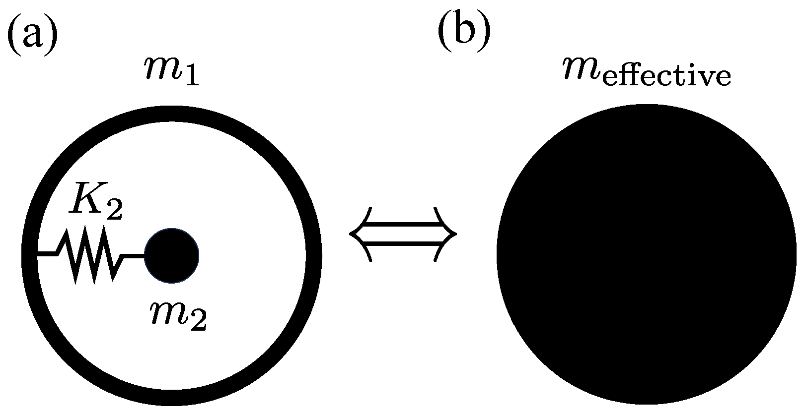
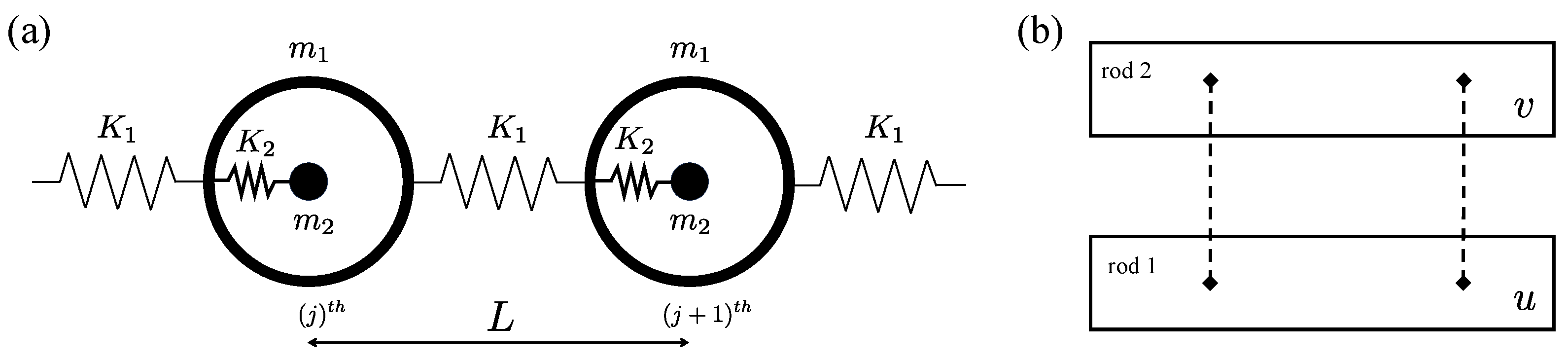
2.4. Mass-in-Mass Systems

The unit cell of a mass-in-mass system is represented in Figure 7. It can be understood with an analogy to the diatomic model (Figure 4), since we can choose a particle as a system of two atoms and consider the displacement of the atoms relative to the center of mass as a (micro-structural) degree of freedom.
As we next see, these mechanical systems show a frequency band gap given in Figure 6. Materials that show this behavior, i.e., a frequency band gap where acoustic/elastic waves do not propagate, are referred to in the literature as seismic metamaterials [58,62,63,91,92,93,94,95,96,97,98,99]. According to [99], there are four main types of seismic metamaterials: (i) seismic soil metamaterials, (ii) buried mass resonators, (iii) above-surface resonators, and (iv) auxetic materials. All are used/designed to trap seismic energy in the frequency range of interest. In the next section, we show that acoustic metamaterials can be understood as mass-in-mass systems.

2.4.1. Acoustic Metamaterials

Figure 7a shows the unit cell created by two masses ( m 1 , m 2 ) connected by a single spring with spring constant K 2 .
One can next construct a continuum connecting the unit cells presented in Figure 7a, by a spring with a spring constant K 1 as presented in Figure 8a.
The lattice equations of motion for this system are given by the following expressions [72]:
m 1 ( j ) t 2 u 1 ( j ) + K 1 2 u 1 ( j ) u 1 ( j 1 ) u 1 ( j + 1 ) + K 2 u 1 ( j ) u 2 ( j ) = 0 , m 2 ( j ) t 2 u 2 ( j ) + K 2 u 2 ( j ) u 1 ( j ) = 0 .
The continuum representation of Equation (29) can be simply found by dividing by the volumes and replacing the finite-difference expression involving u 1 by its Taylor approximation, which results in the following expressions:
ρ 1 t 2 u 1 = μ x 2 u 1 + μ L c 2 u 2 u 1 , ρ 2 t 2 u 2 = μ L c 2 u 1 u 2 ,
where we have simplified the notation and assumed that the two masses occupy the same volume. Ref. [72] found that the continuum approximation Equation (30) was equivalent to the lattice equations of motion, Equation (29), for wavelengths greater than four times the lattice spacing L. Equation (30) can be reduced to a single equation given by Equation (1), where the terms are given by the following expressions:
c x 2 2 = μ ( ρ 1 + ρ 2 ) , c x 4 = 0 , ω r 2 = μ L c 2 1 ρ 1 + 1 ρ 2 , c x t 2 = μ ρ 1 .
Assuming plane-wave propagation in the form of Equation (2), we find the expression for the (squared) phase velocity ( ω / k ) :
ω 2 k 2 = c x 2 2 1 ω 2 / ω 1 2 1 ω 2 / ω r 2 ,
with parameters given in Equation (31) and
ω 1 2 = ρ 1 + ρ 2 ρ 1 ω r 2 .
Note that with the difference in the resonant frequencies ω 1 , ω r , the phase velocity for the mass-in-mass system given in Equation (32) is the same as the one obtained for the reduced micropolar model given in Equation (24). This means that both models can be used to design seismic metamaterials that trap acoustic/elastic waves in a frequency band ( ω 1 , ω r ) of interest.

2.4.2. Theory of Wave Propagation in a Coupled Rod

There exist analogies between wave motion in two rods, connected by elastic springs, and Cosserat’s medium [90]. For the reduced Cosserat medium, instead of two interconnected rods, we have to consider a degenerate case, where one of the rods still exists, but elastic connections in the second rod are destroyed, i.e., the whole system represents an elastic rod (bearing continuum) enhanced at each point by an oscillator (distributed dynamic absorber). This is a reduced continuum, corresponding on the continuum level to the system known in the domain of acoustic metamaterials as a “mass-in-mass” mechanical system [100].
The equations of motion of a system of coupled rods (see Figure 8b) are given by the following expressions [90,101,102]:
ρ 1 S 1 t 2 v = E 1 S 1 x 2 v + R ( w v ) , ρ 2 S 2 t 2 w = R ( v w ) ,
where E i , ρ i , S i are the modulus of elasticity, density, and cross-sectional area of the ith rod, and R is the coefficient of elastic interaction [90]. The fields of motion w and v are displacements of the rods. Note that in this model, the strain energy depends on w , v , x v but does not depend on x w , so we may expect (see [103]) that this medium will behave as a single negative acoustic metamaterial, i.e., it will have a band gap for a certain type of waves, as it takes place for the reduced linear elastic Cosserat medium.
For consistency with our previous analyses, we rewrite the equations of motion in Equation (34) as follows:
ρ 1 t 2 v = μ x 2 v μ L c 2 ( u v ) , ρ 2 t 2 u = μ L c 2 ( v u ) ,
where μ is the shear modulus, and L c is a characteristic length used to define the coefficient of elastic interaction R = μ / L c 2 . It becomes clear that Equations (30) and (35) have the same mathematical structure. This means that both models are equivalent and model the same physics of acoustic metamaterials with a frequency band gap ( ω 1 , ω r ) .

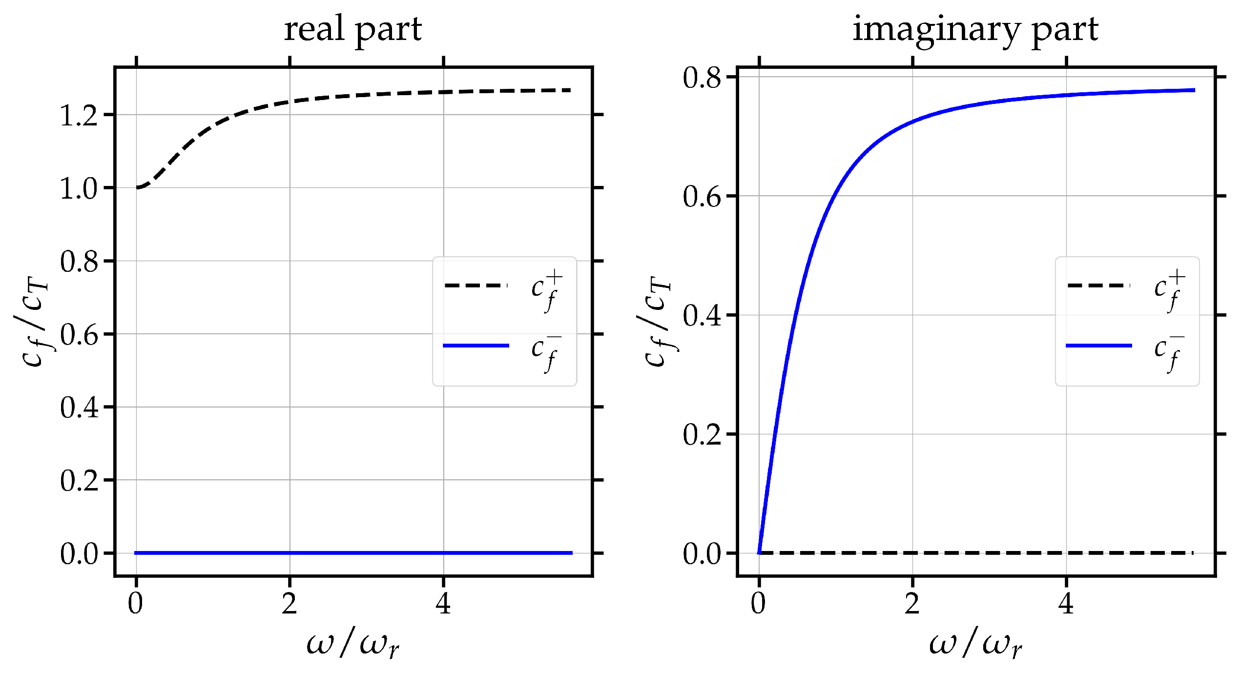
2.5. Micropolar Theory with Gradient Micro-Inertia

The micropolar model with gradient micro-inertia is a variant of the original micropolar model [35]. Like the original micropolar model, it describes a continuum in which additional rotational degrees of freedom θ are present that are different from the rotation computed using the curl of the displacement ( × u ) . The difference, however, is that the independent rotation θ is not an observable but the effective independent rotation ( 1 / 2 × u θ ) is the observable. This means that we are not able to observe/measure θ but the effective rotational motion (or net vorticity) vector Ψ as the difference between the curl of the displacement and the independent rotation as follows
Ψ k = 1 2 ϵ k a b a u b θ k , with a , b , k { 1 , 2 , 3 } ,
where ϵ is the Levi–Civita symbol. The authors in [75] showed that the net vorticity vector Ψ was an objective variable. This means that it is an intrinsic characteristic of the deformation and not simply the effect of rigid rotations of the micro-material.
Assuming shear deformation (transverse displacement ( u ) ) and independent rotational motion ( θ ) , the 1D isotropic micropolar equations with gradient micro-inertia read as follows [35]:
ρ t 2 u = μ x 2 u + 2 μ c x Ψ , I t 2 Ψ = μ L c 2 x 3 u + 4 μ c Ψ ,
where, as usual, u is the displacement vector, ρ the material density, I the micro-inertia density, μ the shear modulus, L c the characteristic length of the problem, and the new variable Ψ the net vorticity. Equation (37) can be reduced to a single equation given by Equation (1), where the terms are given by the following expressions:
c x 2 2 = c x t 2 = μ ρ , c x 4 2 = μ ρ L c 2 2 , ω r 2 = 4 μ c I .
Assuming plane-wave solutions in the form of Equation (2), we can write an expression for the (squared) phase velocity ω / k as follows
ω 2 k 2 = 1 2 c x 2 2 ± c x 2 4 + 4 c x 4 2 ω 2 1 + ω 2 ω r 2 ,
where the terms are given in Equation (38). The phase velocity, for normalized parameters, is given in Figure 9.
We can observe that the are two modes of wave propagation, as in Figure 5; however, only one is visible since the real part of the second one is zero. This can be clearly seen if we assume that I = ρ L c 2 and analyze the following low- and high-frequency limits:
lim ω 0 ω 2 k 2 = lim ω 0 1 2 c x 2 2 ± c x 2 2 c x 2 2 + 2 L c 2 ω 2 1 + ω 2 ω r 2 = c x 2 2 , lim ω ω 2 k 2 = lim ω 1 2 c x 2 2 ± c x 2 2 c x 2 2 + 2 L c 2 ω 2 1 + ω 2 ω r 2 = 1 2 c x 2 2 ± c x 2 2 c x 2 2 + 2 L c 2 ω r 2 .
This means that at low frequencies ( ω 0 ) , there is only one phase velocity c x 2 and at high frequencies ( ω ) , only one phase velocity is real. Therefore, assuming that the net vorticity ( Ψ ) is an objective variable, we can predict acoustic phase velocity dispersion and the presence of only one mode of wave propagation.

2.6. Summary of Theoretical Findings

After this cumbersome presentation of all theoretical models, we summarize in Table 1 each model and its relation to the general PDE given in Equation (1). We can observe that in order to observe a frequency band gap, needed to model seismic metamaterials, one needs to impose that x 4 = 0 . The rest of the models show a general dispersion relation given in Figure 5, and the micropolar model with gradient micro-inertia is the only one where, despite having two modes (acoustic and optic), only one is observable.
We next show realistic applications of our theoretical findings.

3. Applications in Earth Sciences

After establishing some order within the zoo of different theories, we next present applications in Earth sciences. To do so, we only use the micropolar model with gradient micro-inertia [104]. There are two main reasons for this:
  • Earth scientists observe only one mode of propagation. They cannot differentiate between acoustic and optic modes.
  • No frequency band gaps have ever been observed in seismological data.
The fundamental assumption of the micropolar model with gradient micro-inertia is quite simple: only the net vorticity Ψ (Equation (36)) is an observable and an objective variable. One cannot observe separately the individual micro- and macrorotations. This allows us to predict velocity dispersion without any band gaps and/or phase velocities going to zero/infinity (see Figure 9). As a consequence, we can interpret micro- and macroscales as the two limiting (frequency) cases of phase velocity Equations (39) and (40) as follows:
macroscale lim ω 0 ω 2 k 2 = μ ρ = c macro 2 , microscale lim ω ω 2 k 2 = 1 2 μ ρ ± μ ρ μ ρ + 2 L c 2 ω r 2 = c micro 2 .
We can next write a relationship between macroscopic and microscopic phase velocities, by combining them with Equation (41), which results in the following expression:
c micro 2 = 1 2 c macro 2 ± c macro 2 c macro 2 + 2 L c 2 ω r 2 .
After some algebra, using Equation (42), we can write an explicit expression for c macro 2 and ω r L c that results in the following:
c macro 2 = c micro 2 1 1 + 0.5 L c 2 ω r 2 c micro 2 , L c 2 ω r 2 = 2 c micro 2 c macro 2 c micro 2 c macro 2 .
Equations (42) and (43) give a fundamental (mechanical) relationship between micro- and macroscales, both depending on only two parameters: a resonant frequency ω r and a characteristic length L c . In the following, we employ ω r to refer to the angular frequency (rad/s) and f r to refer to the linear frequency (Hz).
To gain some intuition into Equations (42) and (43), let us assume that
c micro = α c macro , with α R + ,
where α is simply a non-dimensional positive scaling factor. Then, we can write the following expression:
α 2 = 1 ± 1 + 2 L c 2 f r 2 / c macro 2 2 ,
where f r [Hz] is the linear frequency. Figure 10 shows the obtained results predicted by Equation (45). We observe that always, c macro < c micro , which can be understood as smaller is always stiffer. The limiting cases are
lim L c ω r 0 α = 1 , lim L c ω r α = ,
which guaranty that L c ω r > 0 in Equation (43).
In the next section, we explore how these concepts can easily be used to model velocity dispersion in granular media in a completely new and simple way.

3.1. Accurate Modeling of Shear-Wave Speed Dispersion in Granular Marine Sediments Without Biot’s Theory

3.1.1. The Problem: Too Many Parameters

Velocity dispersion in marine sediments is one of the important subjects in the field of sediment acoustics [105,106]. It plays a significant role in understanding how elastic waves propagate in the seafloor, affecting applications like underwater communication, sonar performance, and geophysical exploration [107,108,109,110,111].
Marine sediments can be seen as a porous medium composed of a solid matrix filled with fluids. Wave propagation in such media was first described by Biot’s theory [112,113]. A modification of this initial model to better describe marine sediments by taking into account the interaction between solid grains (skeleton) and the pore fluid was made by [114]. This model is known as the Biot–Stoll model and it is widely used today to model wave propagation in marine sediments [115,116,117,118,119].
The Biot–Stoll model possesses a total of thirteen parameters (grain density, grain bulk modulus, fluid density, fluid bulk modulus, porosity, viscosity, permeability, pore size, tortuosity, static-frame shear modulus, grain Poisson’s ratio, asymptotic fluid contribution, and bulk relaxation frequency); however, it is not capable of reproducing detailed observations of shear-wave propagation and attenuation in angular sand [120,121]. In order to reproduce observations, [122,123,124] proposed a modification of the original Biot model called the BIMGS (Biot modified gap stiffness) model. This model possessed, in addition to the thirteen parameters of Biot’s model, a total of four more parameters (Hertz–Mindlin shear modulus, the maximum gap stiffness term of the frame shear modulus, the aspect ratio, and the relaxation frequency).
The large number of parameters required to model seismic wave propagation using the Biot–Stoll (13 parameters) and/or BIMGS models (17 parameters), makes the theories quite unpractical for seismological purposes, since seismologists do not have access to such a large amount of detailed information about the medium. We next show how we can use the micropolar model with gradient micro-inertia to reproduce observations of shear wave dispersion in marine sediments reported in [120,121,122,123,124] and to reduce the seventeen parameters of the BIMGS model to only two parameters.

3.1.2. The Solution: Experimental Validation of the Micropolar Model with Gradient Micro-Inertia

We use shear-wave dispersion measurements performed by [120,121] and reported in [124]. Seventeen different parameters (grain density, grain bulk modulus, fluid density, fluid bulk modulus, porosity, viscosity, permeability, pore size, tortuosity, static-frame shear modulus, grain Poisson’s ratio, asymptotic fluid contribution, and bulk relaxation frequency, Hertz–Mindlin shear modulus, the maximum gap stiffness term of the frame shear modulus, the aspect ratio, and the relaxation frequency) were calculated to match the BIMGS model to experimental phase velocity dispersion curves at three different temperatures [5, 20, 35] °C, in [124].
The fit of the experimental data against the BIMGS model is shown in Figure 11 and the material parameters presented in Table 2. Experimental data indicated that shear velocity increased with frequency and decreased with temperature. We can observe that the BIMGS model fit the data only at certain frequencies measured in the laboratory and that there were two limiting velocities for very low ( f 0 ) and high ( f ) frequencies, that we termed c macro and c micro , respectively. At these two limits, the BIMGS model converged to single values (see Table 2).
In order to reduce the complexity and the number of parameters required by the BIMGS model (seventeen parameters) and to show the applicability of the micropolar model with gradient micro-inertia, we next performed a grid search. In principle, we needed to select only two micropolar parameters, the resonant frequency f r and the characteristic length L c . However, one can note that if we set free the two limiting velocities at f 0 and f , i.e., ( c macro , c micro ) , we can argue that the BIMGS models has nineteen free parameters and the micropolar only four. Thus, for our first parameter search, we set the values of ( c macro , c micro ) to those obtained by the BIMGS model and given in Table 2.
The results of the grid search are presented in Figure 12a–c. We can observe that the micropolar model could reproduce the experimental values while at the same time fitting the macroscopic ( c macro ) and microscopic ( c micro ) phase velocities predicted by the BIMGS model. We obtained a histogram of values of the resonant frequency f r and the characteristic length L c that matched observations.
For visual comparisons between the BIMGS and the micropolar models, we show in Figure 13 the BIMGS model reported by [124] and one fitting micropolar example (we chose the macroscopic c macro and microscopic c micro phase velocities given in Table 2 and the resonant frequency f r and characteristic length L c given by the mode of the histograms in Figure 12). By simple inspection, one can clearly observe that even if both models properly matched experimental data and predicted the same macroscopic ( c macro ) and microscopic ( c micro ) phase velocities, they were not equivalent. The micropolar model reached the microscopic ( c micro ) phase velocity much faster compared to the BIMGS model.
We next performed a complete grid search by leaving free the four micropolar parameters f r , L c , c micro , c macro . The results are presented in Figure 14 where we can observe that all parameters were (relatively) well constrained with values that were clearly concentrated around the mode. We can also observe that the mode of macroscopic ( c macro ) and microscopic ( c micro ) phase velocities did not match the values predicted by the BIMGS model reported in Table 2. This may be explained by the large measurement errors of the experimental data, which allowed a large freedom in the selection of the parameters. The selection of the macroscopic ( c macro ) and microscopic ( c micro ) phase velocities can be exploited from a different point of view, as we next see.

3.2. A Mechanical Link Between Micro- and Macoscales

In seismology, a clear relationship between the microscale (with the term microscale, we refer to the scale related to laboratory studies where elastic parameters are measured) and macroscale (with the term macroscale, we refer to the global Earth scale) is not yet well understood. The purpose of this section is not to give a complete review of the whole techniques that involve scaling from microscales (laboratory experiments) to macroscales (global Earth observations) in seismology, which involves several disciplines like mineralogy, geology, mathematics, and many others (for a discussion, see [14]), but to propose a mechanical scaling methodology based on the micropolar model with gradient micro-inertia proposed by [35]. This is only a mechanical scaling since the proposed methodology is only based on mechanical (observable) properties and not, for example, thermodynamic properties.
We saw in the previous section that the micropolar model with gradient micro-inertia (like BIMGS) predicted single phase velocities at two frequency limits: the macroscopic ( c macro ) limit, when f 0 , and the microscopic ( c micro ) limit, when f . Strictly speaking, there is no limitation on how to physically interpret how small or large these two limiting cases are.
If one looks closely to the scaling law given by Equation (42), we can observe that it has two free parameters: the resonant frequency ω r and the characteristic length L c . Strictly speaking, however, there is only one free parameter, ω r L c , which has units of velocity. This means that the term ω r L c is a constant between two spatial scales that predict the two phase velocities ( c micro , c macro ) .
If we adopt the micropolar model with gradient micro-inertia as a coupling theory between micro/lab and macro/seismological scales as shown in Figure 15, we should be able to predict/model seismic velocities observed at both (micro/macro)scales and/or to obtain information on the characteristic length L c as a function of the resonant frequency ω r (since ω r L c is a constant across scales). The physical assumption made here by the micropolar model with gradient micro-inertia is simple: at microscopic scales, both the independent rotation θ and macroscopic rotation ( × u ) are observable. This is lost at meso- and macroscales, and only the net vorticity Ψ (Equation (36)) is an observable.

3.2.1. The Presence of Bridgmanite in the Lower Mantle

Bridgmanite silicate perovskite ( Mg , Fe ) SiO 3 is one of the most abundant materials in the planet [125]. The structure/unit cell of bridgmanite silicate perovskite ( Mg , Fe ) SiO 3 is given in Figure 1: red circles represent oxygen atoms, orange circles magnesium or iron atoms, and green circles silicon atoms. The silicon atoms are located at the center of the blue SiO6 octahedrons (see aggregate of atoms in Figure 15).
In several Raman spectroscopy experiments of bridgmanite MgSiO 3 , the micropolar and microstretch behaviors of the SiO 6 octahedral structure have been observed (e.g., [126,127,128,129,130,131]). Modes related to the SiO 6 octahedral rocking motion (see [127]) are interpreted as micropolar behavior, and the modes related to pure octahedral deformation involving the tilting or stretching of the SiO6 octahedral structure are interpreted as microstretch behavior [44,48,49,132].

Data

We used the value reported by [9] for bridgmanite, c micro = 7783 m/s at pressures of 120 GPa, which corresponds approximately to 2740 Km Earth’s depth.
To apply Equation (43), we need additional values of the resonant frequency ω r and characteristic length L c . The resonant frequency f r ( SiO 6 octahedral rocking motion) was reported by [127] at a pressure of 150 GPa as f r = 234 [ cm 1 ] and at zero pressure by [128] as f r = 249 [ cm 1 ] . Since the values reported by [9] were at 120 GPa, we simply interpolated the values to obtain f r = 237 [ cm 1 ] . The corresponding frequency ω r is given by
f r [ Hz ] = c light f r [ cm 1 ] = 7.105 × 10 12 [ Hz ] ,
where c light is the speed of light. This value is the cutoff frequency of micro-rotational motions f r in bridgmanite at the required pressure of 120 GPa.
We assumed that macroscopic phase velocities c macro were obtained by seismological observations. We used a total of five different earth models: PREM [133], SP6 [134], IASP91 [135], AK135 [136], and PWDK [137]. We extracted from each model the shear velocity at a depth of 2740 Km.
The characteristic length L c , however, is not a well-constrained parameter. For the calculation of the characteristic length L c , we considered two different scenarios (all values taken from [9]):
  • Average length of the sides of the unit cell:
    L c = 2.471 + 8.091 + 6.110 3 = 5.557 [ Å ]
  • The total volume of the bridgmanite unit cell reported by [9] is of V = 122.16 Å 3 . It is reasonable to assume the unit cell as a cube and take the side of the cube as the characteristic length, from which we can obtain
    L c = V 3 = 4.962 [ Å ]

Results

In order to validate the predictive power of the model, we sought to match the macroscopic phase velocity c macro observed from seismological observations based only on laboratory observations of bridgmanite. The results obtained are presented in Figure 16a, where we can observe that, as expected, results varied depending on the choice of the characteristic length L c . Note that if we took PREM [133] as the reference model, then the c macro results using Equation (43) (for all characteristic lengths) would be within the ± 2 % range. In particular, for the choice of the characteristic length being the average length of the sides of the unit cell (Equation (48)), Equation (43) predicted the seismic velocity predicted by the PWDK model [137]. The PWDK model is a tomographic model that includes the D″ layer. Therefore, one could naturally expect that this would be the model that better matched laboratory experiments.
Having validated the predictive power of our model, we turned our attention to the fact that the term ω r L c , as explained before, is a constant across scales. Figure 16b shows the prediction of the characteristic scale L c for the seismic period band assuming bridgmanite was the material studied. We observed that at 1 s, the characteristic length was L c = 410 m. This means that at 1 s and at conditions of the lower mantle, shear deformation was significant for bridgmanite at ∼400 m. Smaller scales did not sense shear deformations. What this interpretation gives is an intuitive idea on the characteristic scales of the materials at different frequencies, without having to compute/obtain the shear velocity at different P/T conditions.

4. Discussion and Conclusions

4.1. Different Theories: One Equation

We showed that eight different theories (linear elasticity, the lattice model of two atoms per primitive unit cell, micropolar (with and without gradient micro-inertia), reduced micropolar, microstretch, mass-in-mass systems, and wave propagation in a coupled rod), which are used to describe physical phenomena at the micro- and macroscales, belonged to a single general PDE, (or to a particular case of that one), commonly called in the literature as Timoshenko’s equation (Equation (1)). This means that the physical interpretation of Timoshenko’s equation (Equation (1)) can be adapted and/or reinterpreted for each particular physical phenomenon under study.

4.2. Poroelastic Modeling Without Biot’s Theory: The Need for a Simpler Theory in Seismology

We presented a new technique to model shear-wave dispersion in marine sediments without the need to have information and/or to compute the large number of parameters (seventeen) needed by Biot’s theory of wave propagation in porous media and/or its variants. To do so, we relied on the micropolar theory with gradient micro-inertia presented by [35]. This allowed us to reproduce observations with the tuning of only two parameters: the resonant frequency ω r and the characteristic length L c .
This is of particular interest since in realistic seismological scenarios, we do not have access to such a large amount of information required by Biot’s parameters (see Table 2). Instead, seismologists do have access to records of displacements (velocity and/or acceleration) and deformation fields (like gradients and/or rotations), which can be directly modeled with the micropolar theory with gradient micro-inertia with the requirement of only two parameters. This greatly simplifies the realistic modeling of poroelastic effects that can be observed in seismological records.
  • The Meaning of the Resonant Frequency ω r
The resonant frequency ω r can be understood as a reference frequency at which we can observe (strong) shear velocity dispersion (see Figure 9 at ω / ω r = 1 ).
  • The Meaning of the Characteristic Length L c
The characteristic length L c represents the effective length over which shear deformation is significant. This means that it represents the length over which shear deformation dominates. We can think, for example, that the term μ L c behaves like a shear stiffness: a small L c means a stiffer response (less shear deformation) and a large L c means a more flexible response (larger shear deformation).
Using Equation (38), we can write the following expression:
L c = 2 2 c x 4 c x t = 2 2 c x 4 c x 2 .
This means that the characteristic length L c is a scaling factor between the limit of phase (and group) velocity at high frequencies ( c x 4 ) and the limit of phase (and group) velocity at low frequencies ( c x 2 ) and/or the limit of phase (and group) (rotatory) velocity at high frequencies ( c x t ) .

4.3. From Micro- to Macroscales and Vice Versa

Many different methodologies to connect the micro- and macroscales can be adopted. The literature on the topic is vast, and many methods deal with the time/space scaling problem either with homogenization techniques [17,18] or the coupling of different theories [30].
We presented a new methodology to connect shear-wave velocities at micro- ( c micro ) and macroscales ( c macro ) linked by a single factor L c ω r , which consisted of two components: the resonant frequency ω r and the characteristic length L c . If one looks closely, if we convert ω r from an angular frequency to a linear frequency f r , then the units of L c f r are units of velocity [m/s]. This velocity term L c f r remains constant for given micro and macro shear velocities (see Figure 17). This allows us to compute the characteristic length L c that should be observed for a given frequency f r and at the same time, respecting the values of microscopic c micro and macroscopic c macro phase velocities.
We applied this methodology to compute the characteristic length that one would expect at lower mantle conditions close to the CMB. At periods of 1 s, we observed that L c = 0.41 km (see Figure 16b). Comparing this value to the wavelength at 1 s obtained assuming the PWDK model [137], which was ∼7.3 km, we observed that L c was more than one magnitude smaller. This agrees with the concept of the characteristic length L c as a measure of the effective length over which shear deformation is significant. In other words, L c behaves as a measure of the microstructure of the material at which shear deformation is significant.

4.4. Body-Wave Velocity Dispersion Without Viscoelastic Effects

Seismological observations are closely related to the Earth’s internal microstructure, which is believed to produce a natural loss of energy (intrinsic attenuation) through the entire seismic frequency range (0.01–100 Hz) [138,139,140]. This intrinsic attenuation is manifested in seismic records by a coupled effect of physical dispersion and dissipation [141,142,143,144,145].
The mathematical description of the physical mechanism causing the intrinsic attenuation of seismic waves is not yet well understood. Dispersion and dissipation effects are commonly both introduced in wave propagation problems in a coupled way [69]. We showed how to model physical dispersion related to the microstructure without making any assumptions about the loss of energy. This provides a new tool to separate intrinsic (or extrinsic) attenuation and dispersion effects in realistic scenarios, thus providing a deeper understanding of the materials present inside the Earth.

4.5. Bridgmanite in the Lower Mantle

Increasing evidence has been put forth linking the seismic structure of the deepest mantle to overall mantle dynamics and the chemistry of the Earth on a variety of scale lengths [146]. For decades, the general presence of two long-wavelength low-velocity regions at the base of the Earth’s mantle has been observed and studied [147,148,149,150,151,152,153,154,155,156]. The nature of these so-called large low-seismic-velocity provinces (LLSVPs) as well as ultralow-velocity zones (ULVZs) are still not well constrained. Several attempts have been made to explain their structure and origin with the presence of chemical and thermal heterogeneities or of partial melt [146,149,157,158,159,160,161,162,163,164].
Different conforming materials of LLSVPs have been proposed like the discovery of the bridgmanite-to-post-perovskite phase transition in MgSiO3, first announced in April 2004 by [165]. This phase transition is expected to occur for deep mantle conditions and has stimulated numerous studies in experimental and theoretical mineral physics, seismology, and geodynamics evaluating the implications of a major lower-mantle phase change [13,130,131,166,167,168,169]. The progress of high-pressure and high-temperature experimental studies help to elucidate the nature of the discontinuities in the Earth’s mantle.
With the direct link between macroscopic observations and microscopic laboratory experiments, it should be possible to better constrain the Earth’s internal materials. The Earth’s lower most mantle is mostly formed by silicate perovskites [170,171,172,173] and it has been shown that a reduction in shear-wave velocities for perovskites CaSiO3 can be explained by taking into account the rotational relaxation of the SiO6 octahedron [174]. This has been predicted using the density-functional constant-temperature first-principles molecular dynamics method and is in agreement with our findings in Section 2.5.

Funding

This research was partially funded by the DFG (Deutsche Forschungsgemeinschaft) grant number EARLY AB887/1-1.

Data Availability Statement

Data are available upon reasonable request to the corresponding author.

Acknowledgments

R.A. acknowledges initial comments of Jeroen Tromp on micropolar media and constructive continuous conversations with Elena Grekova as well as the constructive comments of three anonymous reviewers. Numerical computations were performed on the S-CAPAD/DANTE platform, IPGP, France.

Conflicts of Interest

The author declares no conflict of interest.

Appendix A. Explicit Calculations: The Lattice Model of Two Atoms per Primitive Unit Cell

In this short appendix, we provide explicit calculations on how to find the general PDE and phase velocity for the lattice model of two atoms per primitive unit cell. The same procedure can be extrapolated to the rest of the models presented in the text. Assuming plane-wave propagation in the form
u ( x , t ) , v ( x , t ) = A , B e i ( k x + ω t ) ,
where A , B are the wave amplitudes, k the wavenumber, and ω the angular frequency and substituting Equation (A1) into the equations of motion, Equation (16), we can write the following expression:
0 = ρ 1 ω 2 A μ B k 2 μ L c i k B + 2 μ L c 2 ( B A ) , 0 = ρ 2 ω 2 B μ A k 2 + μ L c i k A + 2 μ L c 2 ( A B ) .
Equation (A2) can be written as follows:
ρ 1 ω 2 2 μ L c 2 μ k 2 μ L c i k + 2 μ L c 2 μ k 2 + μ L c i k + 2 μ L c 2 ρ 2 ω 2 2 μ L c 2 A B = 0 .
The determinant of Equation (A3) leads to the following expression:
ω 4 μ 2 ρ 1 ρ 2 k 4 + 3 μ 2 ρ 1 ρ 2 L c 2 k 2 2 μ ω 2 L c 2 1 ρ 1 + 1 ρ 2 = 0 .
The PDE corresponding to Equation (A4) is given by the following expression:
t 4 μ 2 ρ 1 ρ 2 x 4 3 μ 2 ρ 1 ρ 2 L c 2 x 2 + 2 μ L c 2 1 ρ 1 + 1 ρ 2 t 2 u , v = 0 .
Equation (A5) is an equivalent non-coupled PDE to the original coupled system of equations of motion in Equation (16). The phase velocity expression can be obtained by taking Equation (A4), dividing it by k 4 , and reordering terms, which results in the following:
ω 4 k 4 1 2 μ ω 2 L c 2 1 ρ 1 + 1 ρ 2 + ω 2 k 2 3 μ 2 ω 2 ρ 1 ρ 2 L c 2 μ 2 ρ 1 ρ 2 = 0 .
Note that Equation (A6) is simply a quadratic equation for ω 2 / k 2 .

References

  1. Bregman, N.; Bailey, R.; Chapman, C. Crosshole seismic tomography. Geophysics 1989, 54, 200–215. [Google Scholar]
  2. Chiao, L.Y.; Kuo, B.Y. Multiscale seismic tomography. Geophys. J. Int. 2001, 145, 517–527. [Google Scholar] [CrossRef]
  3. Tape, C.; Liu, Q.; Maggi, A.; Tromp, J. Seismic tomography of the southern California crust based on spectral-element and adjoint methods. Geophys. J. Int. 2010, 180, 433–462. [Google Scholar]
  4. Nolet, G. A Breviary of Seismic Tomography: Imaging the Interior of the Earth and Sun; Cambridge University Press: Cambridge, UK, 2008. [Google Scholar]
  5. Rawlinson, N.; Pozgay, S.; Fishwick, S. Seismic tomography: A window into deep Earth. Phys. Earth Planet. Inter. 2010, 178, 101–135. [Google Scholar]
  6. French, S.W.; Romanowicz, B.A. Whole-mantle radially anisotropic shear velocity structure from spectral-element waveform tomography. Geophys. J. Int. 2014, 199, 1303–1327. [Google Scholar] [CrossRef]
  7. Lei, W.; Ruan, Y.; Bozdağ, E.; Peter, D.; Lefebvre, M.; Komatitsch, D.; Tromp, J.; Hill, J.; Podhorszki, N.; Pugmire, D. Global adjoint tomography–model GLAD-M25. Geophys. J. Int. 2020, 223, 1–21. [Google Scholar]
  8. Thrastarson, S.; van Herwaarden, D.P.; Noe, S.; Josef Schiller, C.; Fichtner, A. REVEAL: A global full-waveform inversion model. Bull. Seismol. Soc. Am. 2024, 114, 1392–1406. [Google Scholar]
  9. Oganov, A.R.; Ono, S. Theoretical and experimental evidence for a post-perovskite phase of MgSiO3 in Earth’s D′′ layer. Nature 2004, 430, 445–448. [Google Scholar]
  10. Kaminsky, F. Mineralogy of the lower mantle: A review of ‘super-deep’ mineral inclusions in diamond. Earth-Sci. Rev. 2012, 110, 127–147. [Google Scholar]
  11. Irifune, T.; Tsuchiya, T. Mineralogy of the Earth-Phase transitions and mineralogy of the lower mantle. Miner. Phys. 2007, 2, 33–62. [Google Scholar]
  12. Kesson, S.; Fitz Gerald, J.; Shelley, J. Mineralogy and dynamics of a pyrolite lower mantle. Nature 1998, 393, 252–255. [Google Scholar]
  13. Murakami, M.; Ohishi, Y.; Hirao, N.; Hirose, K. A perovskitic lower mantle inferred from high-pressure, high-temperature sound velocity data. Nature 2012, 485, 90–94. [Google Scholar] [PubMed]
  14. Passchier, C.W.; Trouw, R.A.J. Microtectonics; Springer: Berlin/Heidelberg, Germany, 2005. [Google Scholar]
  15. Goetze, C.; Brace, W. The upper mantle laboratory observations of high-temperature rheology of rocks. Tectonophysics 1972, 13, 583–600. [Google Scholar]
  16. Wang, N.; Montagner, J.P.; Fichtner, A.; Capdeville, Y. Intrinsic versus extrinsic seismic anisotropy: The radial anisotropy in reference Earth models. Geophys. Res. Lett. 2013, 40, 4284–4288. [Google Scholar] [CrossRef]
  17. Capdeville, Y.; Zhao, M.; Cupillard, P. Fast Fourier homogenization for elastic wave propagation in complex media. Wave Motion 2015, 54, 170–186. [Google Scholar]
  18. Capdeville, Y.; Guillot, L.; Marigo, J.J. 2-D non-periodic homogenization to upscale elastic media for P–SV waves. Geophys. J. Int. 2010, 182, 903–922. [Google Scholar]
  19. Capdeville, Y.; Cupillard, P.; Singh, S. Chapter Six—An introduction to the two-scale homogenization method for seismology. In Machine Learning in Geosciences; Advances in Geophysics; Moseley, B., Krischer, L., Eds.; Elsevier: Amsterdam, The Netherlands, 2020; Volume 61, pp. 217–306. [Google Scholar]
  20. Hedjazian, N.; Capdeville, Y.; Bodin, T. Multiscale seismic imaging with inverse homogenization. Geophys. J. Int. 2021, 226, 676–691. [Google Scholar]
  21. Capdeville, Y. Homogenization of seismic point and extended sources. Geophys. J. Int. 2021, 226, 1390–1416. [Google Scholar]
  22. Cupillard, P.; Capdeville, Y. Non-periodic homogenization of 3-D elastic media for the seismic wave equation. Geophys. J. Int. 2018, 213, 983–1001. [Google Scholar]
  23. Mainprice, D.; Barruol, G.; Ismaïl, W.B. The seismic anisotropy of the Earth’s mantle: From single crystal to polycrystal. In Earth’s Deep Interior: Mineral Physics and Tomography from the Atomic to the Global Scale; American Geophysical Union: Washington, DC, USA, 2013; pp. 237–264. [Google Scholar]
  24. Nakata, N.; Beroza, G.C. Stochastic characterization of mesoscale seismic velocity heterogeneity in Long Beach, California. Geophys. J. Int. 2015, 203, 2049–2054. [Google Scholar]
  25. Yuen, D.A.; Cserepes, L.; Schroeder, B.A. Mesoscale structures in the transition zone: Dynamical consequences of boundary layer activities. Earth Planets Space 1998, 50, 1035–1045. [Google Scholar]
  26. Capolungo, L.; Spearot, D.; Cherkaoui, M.; McDowell, D.; Qu, J.; Jacob, K. Dislocation nucleation from bicrystal interfaces and grain boundary ledges: Relationship to nanocrystalline deformation. J. Mech. Phys. Solids 2007, 55, 2300–2327. [Google Scholar]
  27. McDowell, D.; Gall, K.; Horstemeyer, M.; Fan, J. Microstructure-based fatigue modeling of cast A356-T6 alloy. Eng. Fract. Mech. 2003, 70, 49–80. [Google Scholar]
  28. McDowell, D.; Dunne, F. Microstructure-sensitive computational modeling of fatigue crack formation. Int. J. Fatigue 2010, 32, 1521–1542. [Google Scholar]
  29. Tucker, G.J.; Tiwari, S.; Zimmerman, J.A.; McDowell, D.L. Investigating the deformation of nanocrystalline copper with microscale kinematic metrics and molecular dynamics. J. Mech. Phys. Solids 2012, 60, 471–486. [Google Scholar]
  30. Wernik, J.; Meguid, S.A. Coupling atomistics and continuum in solids: Status, prospects, and challenges. Int. J. Mech. Mater. Des. 2009, 5, 79. [Google Scholar]
  31. Rudd, R.E.; Broughton, J.Q. Concurrent coupling of length scales in solid state systems. Comput. Simul. Mater. At. Level 2000, 217, 251–291. [Google Scholar]
  32. Rudd, R.E.; Broughton, J.Q. Coarse-grained molecular dynamics and the atomic limit of finite elements. Phys. Rev. B 1998, 58, R5893. [Google Scholar]
  33. Tadmor, E.B.; Ortiz, M.; Phillips, R. Quasicontinuum analysis of defects in solids. Philos. Mag. A 1996, 73, 1529–1563. [Google Scholar]
  34. Eringen, C. Nonlocal Continuum Field Theories; Springer: Berlin/Heidelberg, Germany, 2002. [Google Scholar]
  35. Abreu, R.; Durand, S. Understanding micropolar theory in the Earth sciences I: The eigenfrequency ωr. Pure Appl. Geophys. 2021, 179, 915–932. [Google Scholar]
  36. Slawinski, M. Waves and Rays in Elastic Continua; World Scientific Publishing Company: Singapore, 2010. [Google Scholar]
  37. Eringen, A.C.; Suhubi, E. Nonlinear theory of simple micro-elastic solids—I. Int. J. Eng. Sci. 1964, 2, 189–203. [Google Scholar]
  38. Whitham, G.B. Linear and Nonlinear Waves; John Wiley & Sons: Hoboken, NJ, USA, 1999. [Google Scholar]
  39. Kittel, C. Introduction to Solid State Physics, 8th ed.; John Wiley & Sons: Hoboken, NJ, USA, 2005. [Google Scholar]
  40. Engel, E. Density Functional Theory; Springer: Berlin/Heidelberg, Germany, 2011. [Google Scholar]
  41. Merzbacher, E. Quantum Mechanics; John Wiley & Sons: Hoboken, NJ, USA, 1998. [Google Scholar]
  42. Madeo, A.; Neff, P.; Ghiba, I.D.; Placidi, L.; Rosi, G. Wave propagation in relaxed micromorphic continua: Modeling metamaterials with frequency band-gaps. Contin. Mech. Thermodyn. 2015, 27, 551–570. [Google Scholar]
  43. Eringen, C.; Kafadar, C. Polar Field Theories, Continuum Physics; Academic Press: Cambridge, MA, USA, 1976; Volume IV, pp. 1–75. [Google Scholar]
  44. Eringen, C. Microcontinuum Field Theories I: Foundations and Solids; Springer: Berlin/Heidelberg, Germany, 1999. [Google Scholar]
  45. Grekova, E.; Kulesh, M.; Herman, G. Waves in linear elastic media with microrotations, Part 2: Isotropic reduced Cosserat model. Bull. Seismol. Soc. Am. 2009, 99, 1423–1428. [Google Scholar]
  46. Madeo, A. Generalized Continuum Mechanics and Engineering Applications; Elsevier: Amsterdam, The Netherlands, 2015. [Google Scholar]
  47. Chen, Y.; Lee, J.D.; Eskandarian, A. Atomistic viewpoint of the applicability of microcontinuum theories. Int. J. Solids Struct. 2004, 41, 2085–2097. [Google Scholar]
  48. Abreu, R.; Thomas, C.; Durand, S. Effect of observed micropolar motions on wave propagation in deep Earth minerals. Phys. Earth Planet. Inter. 2018, 276, 215–225. [Google Scholar] [CrossRef]
  49. Pouget, J.; Aşkar, A.; Maugin, G. Lattice model for elastic ferroelectric crystals: Continuum approximation. Phys. Rev. B 1986, 33, 6320. [Google Scholar]
  50. Askar, A. Molecular crystals and the polar theories of the continua. Experimental values of material coefficients for KNO3. Int. J. Eng. Sci. 1972, 10, 293–300. [Google Scholar]
  51. Askar, A. Lattice Dynamical Foundations of Continuum Theories: Elasticity, Piezoelectricity, Viscoelasticity, Plasticity; World Scientific: Singapore, 1986; Volume 2. [Google Scholar]
  52. Matsushima, T.; Saomoto, H.; Tsubokawa, Y.; Yamada, Y. Grain rotation versus continuum rotation during shear deformation of granular assembly. Soils Found. 2003, 43, 95–106. [Google Scholar]
  53. Twiss, R.J. An asymmetric micropolar moment tensor derived from a discrete-block model for a rotating granular substructure. Bull. Seismol. Soc. Am. 2009, 99, 1103–1131. [Google Scholar]
  54. Schwartz, L.M.; Johnson, D.L.; Feng, S. Vibrational modes in granular materials. Phys. Rev. Lett. 1984, 52, 831–834. [Google Scholar]
  55. Merkel, A.; Luding, S. Enhanced micropolar model for wave propagation in ordered granular materials. Int. J. Solids Struct. 2017, 106, 91–105. [Google Scholar] [CrossRef]
  56. Merkel, A.; Tournat, V.; Gusev, V. Experimental evidence of rotational elastic waves in granular phononic crystals. Phys. Rev. Lett. 2011, 107, 225502. [Google Scholar] [CrossRef] [PubMed]
  57. Madeo, A.; Barbagallo, G.; d’Agostino, M.V.; Placidi, L.; Neff, P. First evidence of non-locality in real band-gap metamaterials: Determining parameters in the relaxed micromorphic model. Proc. R. Soc. A Math. Phys. Eng. Sci. 2016, 472, 20160169. [Google Scholar] [CrossRef]
  58. Frenzel, T.; Kadic, M.; Wegener, M. Three-dimensional mechanical metamaterials with a twist. Science 2017, 358, 1072–1074. [Google Scholar] [CrossRef]
  59. Grekova, E.F.; Abreu, R. Isotropic Linear Viscoelastic Reduced Cosserat Medium: An Acoustic Metamaterial and a First Step to Model Geomedium. In New Achievements in Continuum Mechanics and Thermodynamics: A Tribute to Wolfgang H. Müller; Abali, B.E., Altenbach, H., dell’Isola, F., Eremeyev, V.A., Öchsner, A., Eds.; Springer International Publishing: Berlin/Heidelberg, Germany, 2019; pp. 165–185. [Google Scholar]
  60. Rizzi, G.; d’Agostino, M.V.; Voss, J.; Bernardini, D.; Neff, P.; Madeo, A. From frequency-dependent models to frequency-independent enriched continua for mechanical metamaterials. Eur. J. Mech.-A/Solids 2024, 106, 105269. [Google Scholar] [CrossRef]
  61. Demetriou, P.; Rizzi, G.; Madeo, A. Reduced relaxed micromorphic modeling of harmonically loaded metamaterial plates: Investigating boundary effects in finite-size structures. Arch. Appl. Mech. 2024, 94, 81–98. [Google Scholar] [CrossRef]
  62. Voss, J.; Rizzi, G.; Neff, P.; Madeo, A. Modeling a labyrinthine acoustic metamaterial through an inertia-augmented relaxed micromorphic approach. Math. Mech. Solids 2023, 28, 2177–2201. [Google Scholar] [CrossRef]
  63. Rizzi, G.; Neff, P.; Madeo, A. Metamaterial shields for inner protection and outer tuning through a relaxed micromorphic approach. Philos. Trans. R. Soc. A 2022, 380, 20210400. [Google Scholar] [CrossRef]
  64. Neff, P.; Eidel, B.; d’Agostino, M.V.; Madeo, A. Identification of scale-independent material parameters in the relaxed micromorphic model through model-adapted first order homogenization. J. Elast. 2020, 139, 269–298. [Google Scholar] [CrossRef]
  65. Rayleigh, J.W.S.B. The Theory of Sound; Macmillan: New York, NY, USA, 1896; Volume 2. [Google Scholar]
  66. Watts, A.B. Isostasy and Flexure of the Lithosphere; Cambridge University Press: Cambridge, UK, 2001. [Google Scholar]
  67. Timoshenko, S.P. On the correction for shear of the differential equation for transverse vibrations of prismatic bars. London Edinburgh Dublin Philos. Mag. J. Sci. 1921, 41, 744–746. [Google Scholar] [CrossRef]
  68. Oldham, R.D. The constitution of the interior of the Earth, as revealed by earthquakes. Q. J. Geol. Soc. 1906, 62, 456–475. [Google Scholar]
  69. Aki, K.; Richards, P.G. Quantitative Seismology, 2nd ed.; University Science Books: Herndon, VA, USA, 2002. [Google Scholar]
  70. Dahlen, F.; Tromp, J. Theoretical Global Seismology; Princeton University Press: Princeton, NJ, USA, 1998. [Google Scholar]
  71. Thomas, J.W. Numerical Partial Differential Equations: Finite Difference Methods; Springer: Berlin/Heidelberg, Germany, 1995. [Google Scholar]
  72. Huang, H.; Sun, C.; Huang, G. On the negative effective mass density in acoustic metamaterials. Int. J. Eng. Sci. 2009, 47, 610–617. [Google Scholar] [CrossRef]
  73. Teisseyre, R.; Takeo, M.; Majewski, E. Earthquake Source Asymmetry, Structural Media and Rotation Effects; Springer: Berlin/Heidelberg, Germany, 2006. [Google Scholar]
  74. Cosserat, E.; Cosserat, F. Théorie des Corps Déformables; A. Hermann et Fils; Delphenich, D., Translator; Librairie Scientifique: Paris, France, 2009; ISBN 978-27056-6920-1. [Google Scholar]
  75. Twiss, R.J.; Souter, B.J.; Unruh, J.R. The effect of block rotations on the global seismic moment tensor and the patterns of seismic P and T axes. J. Geophys. Res. Solid Earth 1993, 98, 645–674. [Google Scholar]
  76. Gade, M.; Raghukanth, S. Seismic response of reduced micropolar elastic half-space. J. Seismol. 2016, 20, 787–801. [Google Scholar]
  77. Unruh, J.R.; Twiss, R.J.; Hauksson, E. Seismogenic deformation field in the Mojave block and implications for tectonics of the eastern California shear zone. J. Geophys. Res. Solid Earth 1996, 101, 8335–8361. [Google Scholar] [CrossRef]
  78. Unruh, J.; Humphrey, J.; Barron, A. Transtensional model for the Sierra Nevada frontal fault system, eastern California. Geology 2003, 31, 327. [Google Scholar]
  79. Lewis, J.C.; Boozer, A.C.; López, A.; Montero, W. Collision versus sliver transport in the hanging wall at the Middle America subduction zone: Constraints from background seismicity in central Costa Rica. Geochem. Geophys. Geosyst. 2008, 9, Q07S06. [Google Scholar]
  80. Twiss, R.J.; Protzman, G.M.; Hurst, S.D. Theory of slickenline patterns based on the velocity gradient tensor and micro-rotation. Tectonophysics 1991, 186, 215–239. [Google Scholar]
  81. Lewis, J.C.; O’Hara, D.J.; Rau, R.J. Seismogenic strain across the transition from fore-arc slivering to collision in southern Taiwan. J. Geophys. Res. Solid Earth 2015, 120, 4539–4555. [Google Scholar] [CrossRef]
  82. Neff, P.; Jeong, J. A new paradigm: The linear isotropic Cosserat model with conformally invariant curvature energy. Z. Angew. Math. Mech. 2009, 89, 107–122. [Google Scholar]
  83. Neff, P.; Jeong, J.; Fischle, A. Stable identification of linear isotropic Cosserat parameters: Bounded stiffness in bending and torsion implies conformal invariance of curvature. Acta Mech. 2010, 211, 237–249. [Google Scholar]
  84. Neff, P.; Jeong, J.; Münch, I.; Ramézani, H. Linear Cosserat elasticity, conformal curvature and bounded stiffness. In Mechanics of Generalized Continua: One Hundred Years After the Cosserats; Maugin, G.A., Metrikine, A.V., Eds.; Springer: Berlin/Heidelberg, Germany, 2010; pp. 55–63. [Google Scholar]
  85. Abreu, R.; Kamm, J.; Reiß, A.S. Micropolar modelling of rotational waves in seismology. Geophys. J. Int. 2017, 210, 1021–1046. [Google Scholar]
  86. Kulesh, M.; Grekova, E.; Shardakov, I. The problem of surface wave propagation in a reduced Cosserat medium. Acoust. Phys. 2009, 55, 218–226. [Google Scholar] [CrossRef]
  87. Grekova, E. Linear reduced Cosserat medium with spherical tensor of inertia, where rotations are not observed in experiment. Mech. Solids 2012, 47, 538–543. [Google Scholar]
  88. Grekova, E. Nonlinear isotropic elastic reduced Cosserat continuum as a possible model for geomedium and geomaterials. Spherical prestressed state in the semilinear material. J. Seismol. 2012, 16, 695–707. [Google Scholar]
  89. Grekova, E. Plane waves in the linear elastic reduced Cosserat medium with a finite axially symmetric coupling between volumetric and rotational strains. Math. Mech. Solids 2016, 21, 73–93. [Google Scholar]
  90. Erofeev, V.I.; Malkhanov, A.O. Macromechanical modelling of elastic and visco-elastic Cosserat continuum. J. Appl. Math. Mech. 2017, 97, 1072–1077. [Google Scholar]
  91. Liu, Y.f.; Huang, J.k.; Li, Y.g.; Shi, Z.f. Trees as large-scale natural metamaterials for low-frequency vibration reduction. Constr. Build. Mater. 2019, 199, 737–745. [Google Scholar]
  92. Muhammad; Lim, C.W. Natural seismic metamaterials: The role of tree branches in the birth of Rayleigh wave bandgap for ground born vibration attenuation. Trees 2021, 35, 1299–1315. [Google Scholar] [CrossRef]
  93. Frenzel, T.; Köpfler, J.; Jung, E.; Kadic, M.; Wegener, M. Ultrasound experiments on acoustical activity in chiral mechanical metamaterials. Nat. Commun. 2019, 10, 3384. [Google Scholar]
  94. Miniaci, M.; Krushynska, A.; Bosia, F.; Pugno, N.M. Large scale mechanical metamaterials as seismic shields. New J. Phys. 2016, 18, 083041. [Google Scholar] [CrossRef]
  95. Wu, W.; Hu, W.; Qian, G.; Liao, H.; Xu, X.; Berto, F. Mechanical design and multifunctional applications of chiral mechanical metamaterials: A review. Mater. Des. 2019, 180, 107950. [Google Scholar] [CrossRef]
  96. Chen, Y.; Frenzel, T.; Guenneau, S.; Kadic, M.; Wegener, M. Mapping acoustical activity in 3D chiral mechanical metamaterials onto micropolar continuum elasticity. J. Mech. Phys. Solids 2020, 137, 103877. [Google Scholar] [CrossRef]
  97. Liu, X.; Hu, G. Elastic metamaterials making use of chirality: A review. Stroj. Vestn.-J. Mech. Eng. 2016, 62, 403–418. [Google Scholar] [CrossRef]
  98. Brûlé, S.; Javelaud, E.; Enoch, S.; Guenneau, S. Experiments on seismic metamaterials: Molding surface waves. Phys. Rev. Lett. 2014, 112, 133901. [Google Scholar] [CrossRef]
  99. Brûlé, S.; Enoch, S.; Guenneau, S. Emergence of seismic metamaterials: Current state and future perspectives. Phys. Lett. A 2020, 384, 126034. [Google Scholar] [CrossRef]
  100. Porubov, A.; Grekova, E. On nonlinear modeling of an acoustic metamaterial. Mech. Res. Commun. 2020, 103, 103464. [Google Scholar] [CrossRef]
  101. Meng, J. Coupled Wave Propagation in a Rod with a Dynamic Absorber Layer. Master’s Thesis, Massachusetts Institute of Technology, Cambridge, MA, USA, 1991. [Google Scholar]
  102. Chen, J.S.; Wang, R.T. Wave propagation and power flow analysis of sandwich structures with internal absorbers. J. Vib. Acoust. 2014, 136, 041003. [Google Scholar] [CrossRef]
  103. Grekova, E.F. On one class of theoretically constructed isotropic single negative continuous acoustic metamaterials. In Proceedings of the International Conference Days on Diffraction 2014, St. Petersburg, Russia, 26–30 May 2014; IEEE: New York, NY, USA, 2014; pp. 101–106. [Google Scholar]
  104. Abreu, R.; Durand, S. Understanding micropolar theory in the Earth sciences II: The seismic moment tensor. Pure Appl. Geophys. 2021, 178, 4325–4343. [Google Scholar] [CrossRef]
  105. Stoll, R.D. Velocity dispersion in water-saturated granular sediment. J. Acoust. Soc. Am. 2002, 111, 785–793. [Google Scholar] [CrossRef]
  106. Williams, K.L.; Jackson, D.R.; Thorsos, E.I.; Tang, D.; Schock, S.G. Comparison of sound speed and attenuation measured in a sandy sediment to predictions based on the Biot theory of porous media. IEEE J. Ocean. Eng. 2002, 27, 413–428. [Google Scholar] [CrossRef]
  107. Ballard, M.S.; Lee, K. The acoustics of marine sediments. Acoust. Today 2017, 13, 11–18. [Google Scholar]
  108. Kimura, M. Grain-size dependence of shear wave speed dispersion and attenuation in granular marine sediments. J. Acoust. Soc. Am. 2014, 136, EL53–EL59. [Google Scholar]
  109. Turgut, A.; Yamamoto, T. In situ measurements of velocity dispersion and attenuation in New Jersey Shelf sediments. J. Acoust. Soc. Am. 2008, 124, EL122–EL127. [Google Scholar]
  110. Yu, P.F.; Jiang, J.M.; Geng, J.H.; Zhang, B.J. Shear wave velocity inversion of marine sediments using deep-water OBS Scholte-wave data. Appl. Geophys. 2024, 21, 13–30. [Google Scholar] [CrossRef]
  111. Kugler, S.; Bohlen, T.; Forbriger, T.; Bussat, S.; Klein, G. Scholte-wave tomography for shallow-water marine sediments. Geophys. J. Int. 2007, 168, 551–570. [Google Scholar]
  112. Biot, M.A. Theory of elastic waves in a fluid-saturated porous solid. I. Low frequency range. J. Acoust. Soc. Am. 1956, 28, 168–178. [Google Scholar]
  113. Biot, M. Theory of elastic waves in a fluid-saturated porous solid. II. Higher frequency range. J. Acoust. Soc. Am. 1956, 28, 179–191. [Google Scholar] [CrossRef]
  114. Stoll, R.D. Acoustic waves in ocean sediments. Geophysics 1977, 42, 715–725. [Google Scholar] [CrossRef]
  115. Chotiros, N.P.; Isakson, M.J. A broadband model of sandy ocean sediments: Biot–Stoll with contact squirt flow and shear drag. J. Acoust. Soc. Am. 2004, 116, 2011–2022. [Google Scholar] [CrossRef]
  116. Attenborough, K. Pore Shape and the Biot-Stoll Model for Saturated Sediments. In Ocean Seismo-Acoustics: Low-Frequency Underwater Acoustics; Akal, T., Berkson, J.M., Eds.; Springer: New York, NY, USA, 1986; pp. 435–444. [Google Scholar]
  117. Holland, C.W.; Brunson, B.A. The Biot–Stoll sediment model: An experimental assessment. J. Acoust. Soc. Am. 1988, 84, 1437–1443. [Google Scholar]
  118. Badiey, M.; Cheng, A.H.; Mu, Y. From geology to geoacoustics—Evaluation of Biot–Stoll sound speed and attenuation for shallow water acoustics. J. Acoust. Soc. Am. 1998, 103, 309–320. [Google Scholar]
  119. Shin, H.C.; Taherzadeh, S.; Attenborough, K.; Whalley, W.; Watts, C. Non-invasive characterization of pore-related and elastic properties of soils in linear Biot–Stoll theory using acoustic-to-seismic coupling. Eur. J. Soil Sci. 2013, 64, 308–323. [Google Scholar]
  120. Brunson, B.A. Shear Wave Attenuation in Unconsolidated Laboratory Sediments. Ph.D. Thesis, Oregon State University, Corvallis, OR, USA, 1984. [Google Scholar]
  121. Brunson, B.A. Shear wave attenuation in unconsolidated laboratory sediments. In Shear Waves in Marine Sediments; Springer: Berlin/Heidelberg, Germany, 1991; pp. 141–147. [Google Scholar]
  122. Kimura, M. Frame bulk modulus of porous granular marine sediments. J. Acoust. Soc. Am. 2006, 120, 699–710. [Google Scholar]
  123. Kimura, M. Experimental validation and applications of a modified gap stiffness model for granular marine sediments. J. Acoust. Soc. Am. 2008, 123, 2542–2552. [Google Scholar]
  124. Kimura, M. Shear wave speed dispersion and attenuation in granular marine sediments. J. Acoust. Soc. Am. 2013, 134, 144–155. [Google Scholar]
  125. Tschauner, O.; Ma, C.; Beckett, J.R.; Prescher, C.; Prakapenka, V.B.; Rossman, G.R. Discovery of bridgmanite, the most abundant mineral in Earth, in a shocked meteorite. Science 2014, 346, 1100–1102. [Google Scholar]
  126. Hemley, R.; Jackson, M.; Gordon, R. Theoretical study of the structure, lattice dynamics, and equations of state of perovskite-type MgSiO3 and CaSiO3. Phys. Chem. Miner. 1987, 14, 2–12. [Google Scholar]
  127. Karki, B.; Wentzcovitch, R.; De Gironcoli, S.; Baroni, S. Ab initio lattice dynamics of MgSiO3 perovskite at high pressure. Phys. Rev. B 2000, 62, 14750. [Google Scholar]
  128. Durben, D.J.; Wolf, G.H. High-temperature behavior of metastable MgSiO3 perovskite: A Raman spectroscopic study. Am. Mineral. 1992, 77, 890–893. [Google Scholar]
  129. Chopelas, A. Thermal expansivity of lower mantle phases MgO and MgSiO3 perovskite at high pressure derived from vibrational spectroscopy. Phys. Earth Planet. Inter. 1996, 98, 3–15. [Google Scholar] [CrossRef]
  130. Williams, Q.; Jeanloz, R.; McMillan, P. Vibrational spectrum of MgSiO3 perovskite: Zero-pressure Raman and mid-infrared spectra to 27 GPa. J. Geophys. Res. Solid Earth 1987, 92, 8116–8128. [Google Scholar] [CrossRef]
  131. Shim, S.H.; Kubo, A.; Duffy, T.S. Raman spectroscopy of perovskite and post-perovskite phases of MgGeO3 to 123 GPa. Earth Planet. Sci. Lett. 2007, 260, 166–178. [Google Scholar] [CrossRef]
  132. Pouget, J.; Aşkar, A.; Maugin, G. Lattice model for elastic ferroelectric crystals: Microscopic approach. Phys. Rev. B 1986, 33, 6304. [Google Scholar] [CrossRef]
  133. Dziewonski, A.M.; Anderson, D.L. Preliminary reference Earth model. Phys. Earth Planet. Inter. 1981, 25, 297–356. [Google Scholar] [CrossRef]
  134. Morelli, A.; Dziewonski, A.M. Body wave traveltimes and a spherically symmetric P-and S-wave velocity model. Geophys. J. Int. 1993, 112, 178–194. [Google Scholar] [CrossRef]
  135. Kennett, B.; Engdahl, E. Traveltimes for global earthquake location and phase identification. Geophys. J. Int. 1991, 105, 429–465. [Google Scholar] [CrossRef]
  136. Kennett, B.L.; Engdahl, E.; Buland, R. Constraints on seismic velocities in the Earth from traveltimes. Geophys. J. Int. 1995, 122, 108–124. [Google Scholar] [CrossRef]
  137. Weber, M.; Davis, J. Evidence of a laterally variable lower mantle structure from P-and S-waves. Geophys. J. Int. 1990, 102, 231–255. [Google Scholar] [CrossRef]
  138. Liu, H.P.; Anderson, D.L.; Kanamori, H. Velocity dispersion due to anelasticity; implications for seismology and mantle composition. Geophys. J. Int. 1976, 47, 41–58. [Google Scholar] [CrossRef]
  139. Kjartansson, E. Constant Q–wave propagation and attenuation. J. Geophys. Res. Solid Earth 1979, 84, 4737–4748. [Google Scholar]
  140. Romanowicz, B. Attenuation Tomography of the Earth’s Mantle: A Review of Current Status. In Q of the Earth: Global, Regional, and Laboratory Studies; Mitchell, B.J., Romanowicz, B., Eds.; Birkhäuser: Basel, Switzerland, 1999; pp. 257–272. [Google Scholar]
  141. Zhu, H.; Bozdağ, E.; Duffy, T.S.; Tromp, J. Seismic attenuation beneath Europe and the North Atlantic: Implications for water in the mantle. Earth Planet. Sci. Lett. 2013, 381, 1–11. [Google Scholar]
  142. Durand, S.; Matas, J.; Ford, S.; Ricard, Y.; Romanowicz, B.; Montagner, J.P. Insights from ScS–S measurements on deep mantle attenuation. Earth Planet. Sci. Lett. 2013, 374, 101–110. [Google Scholar] [CrossRef]
  143. Widmer, R.; Masters, G.; Gilbert, F. Spherically symmetric attenuation within the Earth from normal mode data. Geophys. J. Int. 1991, 104, 541. [Google Scholar]
  144. Bezada, M.J. Insights into the lithospheric architecture of Iberia and Morocco from teleseismic body-wave attenuation. Earth Planet. Sci. Lett. 2017, 478, 14–26. [Google Scholar] [CrossRef]
  145. Ford, S.R.; Garnero, E.J.; Thorne, M.S. Differential t* measurements via instantaneous frequency matching: Observations of lower mantle shear attenuation heterogeneity beneath western Central America. Geophys. J. Int. 2012, 189, 513–523. [Google Scholar]
  146. Garnero, E.J.; Thorne, M.S.; McNamara, A.; Rost, S. Fine-Scale Ultra-Low Velocity Zone Layering at the Core-Mantle Boundary and Superplumes. In Superplumes: Beyond Plate Tectonics; Yuen, D.A., Maruyama, S., Karato, S.I., Windley, B.F., Eds.; Springer: Dordrecht, The Netherlands, 2007; pp. 139–158. [Google Scholar]
  147. McNamara, A.K. A review of large low shear velocity provinces and ultra low velocity zones. Tectonophysics 2019, 760, 199–220. [Google Scholar]
  148. Romanowicz, B. Seismic tomography of the Earth’s mantle. Annu. Rev. Earth Planet. Sci. 1991, 19, 77–99. [Google Scholar] [CrossRef]
  149. Frost, D.A.; Rost, S. The P-wave boundary of the large-low shear velocity province beneath the Pacific. Earth Planet. Sci. Lett. 2014, 403, 380–392. [Google Scholar] [CrossRef]
  150. Torsvik, T.H.; Smethurst, M.A.; Burke, K.; Steinberger, B. Large igneous provinces generated from the margins of the large low-velocity provinces in the deep mantle. Geophys. J. Int. 2006, 167, 1447–1460. [Google Scholar]
  151. Burke, K.; Steinberger, B.; Torsvik, T.H.; Smethurst, M.A. Plume generation zones at the margins of large low shear velocity provinces on the core–mantle boundary. Earth Planet. Sci. Lett. 2008, 265, 49–60. [Google Scholar]
  152. Tanaka, S.; Suetsugu, D.; Shiobara, H.; Sugioka, H.; Kanazawa, T.; Fukao, Y.; Barruol, G.; Reymond, D. On the vertical extent of the large low shear velocity province beneath the South Pacific Superswell. Geophys. Res. Lett. 2009, 36, L07305. [Google Scholar]
  153. Steinberger, B.; Torsvik, T.H. A geodynamic model of plumes from the margins of Large Low Shear Velocity Provinces. Geochem. Geophys. Geosyst. 2012, 13, Q01W09. [Google Scholar]
  154. Ballmer, M.D.; Schumacher, L.; Lekic, V.; Thomas, C.; Ito, G. Compositional layering within the large low shear-wave velocity provinces in the lower mantle. Geochem. Geophys. Geosyst. 2016, 17, 5056–5077. [Google Scholar]
  155. Deschamps, F.; Cobden, L.; Tackley, P.J. The primitive nature of large low shear-wave velocity provinces. Earth Planet. Sci. Lett. 2012, 349, 198–208. [Google Scholar]
  156. Dziewonski, A.M.; Hager, B.H.; O’Connell, R.J. Large-scale heterogeneities in the lower mantle. J. Geophys. Res. 1977, 82, 239–255. [Google Scholar]
  157. Thorne, M.S.; Zhang, Y.; Ritsema, J. Evaluation of 1-D and 3-D seismic models of the Pacific lower mantle with S, SKS, and SKKS traveltimes and amplitudes. J. Geophys. Res. Solid Earth 2013, 118, 985–995. [Google Scholar]
  158. Williams, Q.; Garnero, E.J. Seismic evidence for partial melt at the base of Earth’s mantle. Science 1996, 273, 1528–1530. [Google Scholar]
  159. Ni, S.; Helmberger, D.V. Probing an ultra-low velocity zone at the core mantle boundary with P and S waves. Geophys. Res. Lett. 2001, 28, 2345–2348. [Google Scholar]
  160. Wen, L.; Helmberger, D.V. Ultra-low velocity zones near the core-mantle boundary from broadband PKP precursors. Science 1998, 279, 1701–1703. [Google Scholar]
  161. Kawai, K.; Geller, R.J. Waveform inversion for localized seismic structure and an application to D” structure beneath the Pacific. J. Geophys. Res. Solid Earth 2010, 115, B01305. [Google Scholar]
  162. Yao, J.; Wen, L. Seismic structure and ultra-low velocity zones at the base of the Earth’s mantle beneath Southeast Asia. Phys. Earth Planet. Inter. 2014, 233, 103–111. [Google Scholar]
  163. Thorne, M.S.; Garnero, E.J.; Jahnke, G.; Igel, H.; McNamara, A.K. Mega ultra low velocity zone and mantle flow. Earth Planet. Sci. Lett. 2013, 364, 59–67. [Google Scholar] [CrossRef]
  164. Zhang, Y.; Ritsema, J.; Thorne, M.S. Modeling the ratios of SKKS and SKS amplitudes with ultra-low velocity zones at the core-mantle boundary. Geophys. Res. Lett. 2009, 36, L19303. [Google Scholar] [CrossRef]
  165. Murakami, M.; Hirose, K.; Kawamura, K.; Sata, N.; Ohishi, Y. Post-perovskite phase transition in MgSiO3. Science 2004, 304, 855–858. [Google Scholar] [PubMed]
  166. Hirose, K.; Brodholt, J.; Lay, T.; Yuen, D. Post-Perovskite: The Last Mantle Phase Transition; John Wiley & Sons: Hoboken, NJ, USA, 2013; Volume 174. [Google Scholar]
  167. Shim, S.H. The postperovskite transition. Annu. Rev. Earth Planet. Sci. 2008, 36, 569–599. [Google Scholar]
  168. Tateno, S.; Hirose, K.; Sata, N.; Ohishi, Y. Determination of post-perovskite phase transition boundary up to 4400 K and implications for thermal structure in D″ layer. Earth Planet. Sci. Lett. 2009, 277, 130–136. [Google Scholar] [CrossRef]
  169. Tsuchiya, T.; Tsuchiya, J. Effect of impurity on the elasticity of perovskite and postperovskite: Velocity contrast across the postperovskite transition in (Mg, Fe, Al)(Si, Al) O3. Geophys. Res. Lett. 2006, 33. [Google Scholar]
  170. McDonough, W.F.; Sun, S.S. The composition of the Earth. Chem. Geol. 1995, 120, 223–253. [Google Scholar]
  171. Helffrich, G.R.; Wood, B.J. The Earth’s mantle. Nature 2001, 412, 501. [Google Scholar]
  172. Wicks, J.K.; Duffy, T.S. Crystal Structures of Minerals in the Lower Mantle. In Deep Earth; American Geophysical Union (AGU): Washington, DC, USA, 2016; Chapter 6; pp. 69–87. [Google Scholar]
  173. Frost, D.J.; Myhill, R. Chemistry of the Lower Mantle. In Deep Earth; American Geophysical Union (AGU): Washington, DC, USA, 2016; Chapter 18; pp. 225–240. [Google Scholar]
  174. Kawai, K.; Tsuchiya, T. Small shear modulus of cubic CaSiO3 perovskite. Geophys. Res. Lett. 2015, 42, 2718–2726. [Google Scholar] [CrossRef]
Figure 2. Schematic representation of the theoretical separation of length and time scales. After [30].
Geosciences 15 00124 g002
Figure 3. (a) Drawing representing deformation in linear elasticity. (b) Drawing representing a micro-continuum deformation showing the existence of micro-rotation (after [35]).
Geosciences 15 00124 g003
Figure 4. Schematic representations of (a) the single-atom lattice model, (b) the motion of the single-atomic lattice model, (c) the diatomic lattice model with colors representing two different atoms, and (d) the motion of the diatomic lattice model with colors representing two different atoms. Arrows refer to the direction of motion of each particle.
Geosciences 15 00124 g004
Figure 5. Non-dimensional phase velocity ( ω / k = c f ) plot for the general model given by Equation (1). Note that the mode corresponding to c f has zero imaginary part.
Geosciences 15 00124 g005
Figure 6. Non-dimensional phase velocity plot for the reduced micropolar model (Equation (24)).
Geosciences 15 00124 g006
Figure 7. (a) Unit cell of an acoustic metamaterial with two different masses m 1 , m 2 and spring constant K 2 . (b) Homogenization of the unit cell shown in (a) with a negative effective mass.
Geosciences 15 00124 g007
Figure 8. (a) Acoustic metamaterial represented by a mass-in-mass system made of unit cells shown in Figure 7 and connected by a spring ( K 1 ) . (b) Longitudinal deformations of a rod with an elastic (dynamic) coupling.
Geosciences 15 00124 g008
Figure 9. Non-dimensional phase velocity plot for the micropolar model with gradient micro-inertia (Equation (37)).
Geosciences 15 00124 g009
Figure 10. Scaling parameter α (with c micro = α c macro , Equation (44)) as a function of L c 2 f r 2 / c macro 2 (see Equation (45)).
Geosciences 15 00124 g010
Figure 11. Measured and calculated shear-wave speeds in water-saturated silica sand at temperatures of [5, 20, 35] °C as a function of frequency. The calculations were performed using the BIMGS model [124].
Geosciences 15 00124 g011
Figure 12. Grid search inversion using the micropolar phase velocity (Equation (39)) when fixing the macroscopic ( c macro ) and microscopic ( c micro ) phase velocities obtained by [124] and leaving free the resonant frequency ω r and characteristic length L c . Comparison against measured shear-wave speeds in water-saturated silica sand at temperatures of [5, 20, 35] °C (columns (ac)) as a function of frequency [124]. In every plot, the mode is represented by a vertical dotted line.
Geosciences 15 00124 g012
Figure 13. Measured shear-wave speeds in water-saturated silica sand at temperatures of [5, 20, 35] °C as a function of frequency compared to predictions made by the micropolar model (a,b) and the BIMGS [124] model (b). Values used for the micropolar model are given by the mode in Figure 12.
Geosciences 15 00124 g013
Figure 14. Grid search inversion using the micropolar phase velocity (Equation (39)) when leaving free all four parameters ( f r , L c , c micro , c macro ) . Comparison against measured shear-wave speeds in water-saturated silica sand at temperatures of [5, 20, 35] °C (columns (ac)) as a function of frequency [124]. In every plot, the mode is represented by a vertical dotted line.
Geosciences 15 00124 g014
Figure 15. Connections between micro-, meso-, and macroscales and theoretical equivalences. Colors of the macroscopic object (Earth) represent different random materials and on the right an aggregate of atoms that represent the structure of bridgmanite silicate perovskite ( Mg , Fe ) SiO 3 : Red circles represent oxygen atoms, orange circles magnesium or iron atoms and green circles silicon atoms. The silicon atoms are located at the centre of the blue SiO 6 octahedrons.
Geosciences 15 00124 g015
Figure 16. (a) Shear-wave velocity predictions at the lower mantle (depth 2740 km) using Equation (43) and comparison against different tomographic models. (b) Characteristic length L c predicted for the seismic period band assuming the material was bridgmanite.
Geosciences 15 00124 g016
Figure 17. Non-dimensional shear phase curve showing how the value of L c f r is a constant for a given microscopic c micro and macroscopic c macro phase velocities.
Geosciences 15 00124 g017
Table 1. Different model comparisons.
Model t 4 t 2 x 2 x 4 t 2 x 2
Linear elasticity
Diatomic
Micropolar
Reduced micropolar
Microstretch
Mass in mass
Coupled rod
Micropolar (gradient micro-inertia)
Table 2. Parameters of the BIMGS model used in the calculations for the shear-wave speed dispersion and attenuation in water-saturated silica sand [124].
Parameter 5 °C20 °C35 °C
GrainDiameterd [mm]0.1130.1130.113
Density ρ r [kg/m3]265926592659
Bulk modulus K r [Pa] 3.60 × 10 10 3.60 × 10 10 3.60 × 10 10
Pore fluidDensity ρ f [kg/m3]1000998.2994
Bulk modulus K f [Pa] 2.034 × 10 9 2.193 × 10 9 2.296 × 10 9
Viscosity η [Pa s] 1.520 × 10 3 1.002 × 10 3 0.723 × 10 3
FramePorosity β 0.3680.3680.368
Permeability κ [m2] 6.423 × 10 12 6.423 × 10 12 6.423 × 10 12
Pore size a p [m] 2.193 × 10 5 2.193 × 10 5 2.193 × 10 5
Structure factor α t 1.861.861.86
(Biot–Stoll)Frame’s shear modulus μ b [Pa] 7.8 × 10 7 5.8 × 10 7 3.73 × 10 7
Shear log decrement δ s 0.120.120.12
Reference frequency f c [KHz]13.869.156.63
(BIMGS)Hertz–Mindlin shear modulus μ b H M [Pa] 7.80 × 10 7 5.80 × 10 7 3.73 × 10 7
Maximum gap stiffness term of the frame’s shear modulus μ b g [Pa] 8.57 × 10 7 7.96 × 10 7 7.11 × 10 7
Aspect ratio α 4.19 × 10 4 4.19 × 10 4 4.19 × 10 4
Correction factor for attenuation C a 0.170.140.20
Relaxation frequency f r [KHz]19.5832.0246.46
Calculated shear wave speed at f = 0   ( c macro ) c s ( f = 0 ) [m/s]195.1168.3135.0
Calculated shear wave speed at f =   ( c micro ) c s ( f = ) [m/s]297.4272.7242.0
Disclaimer/Publisher’s Note: The statements, opinions and data contained in all publications are solely those of the individual author(s) and contributor(s) and not of MDPI and/or the editor(s). MDPI and/or the editor(s) disclaim responsibility for any injury to people or property resulting from any ideas, methods, instructions or products referred to in the content.

