
Comparison of Seismic Site Factor Models Based on Equivalent Linear and Nonlinear Analyses and Correction Factors for Updating Equivalent Linear Results for Charleston, South Carolina

 , , and
Abstract
1. Introduction
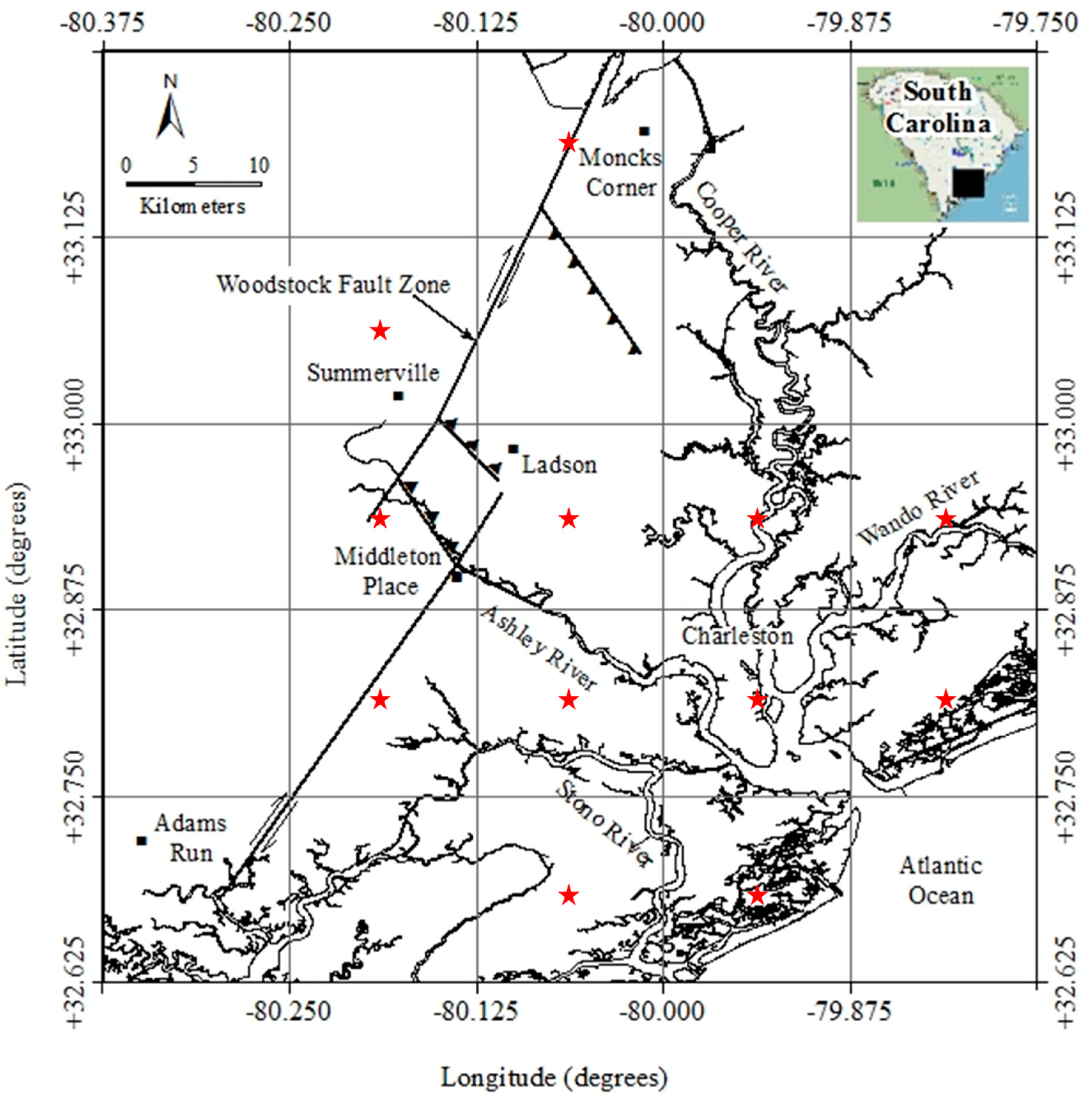
2. Charleston, SC, Geology and Seismology
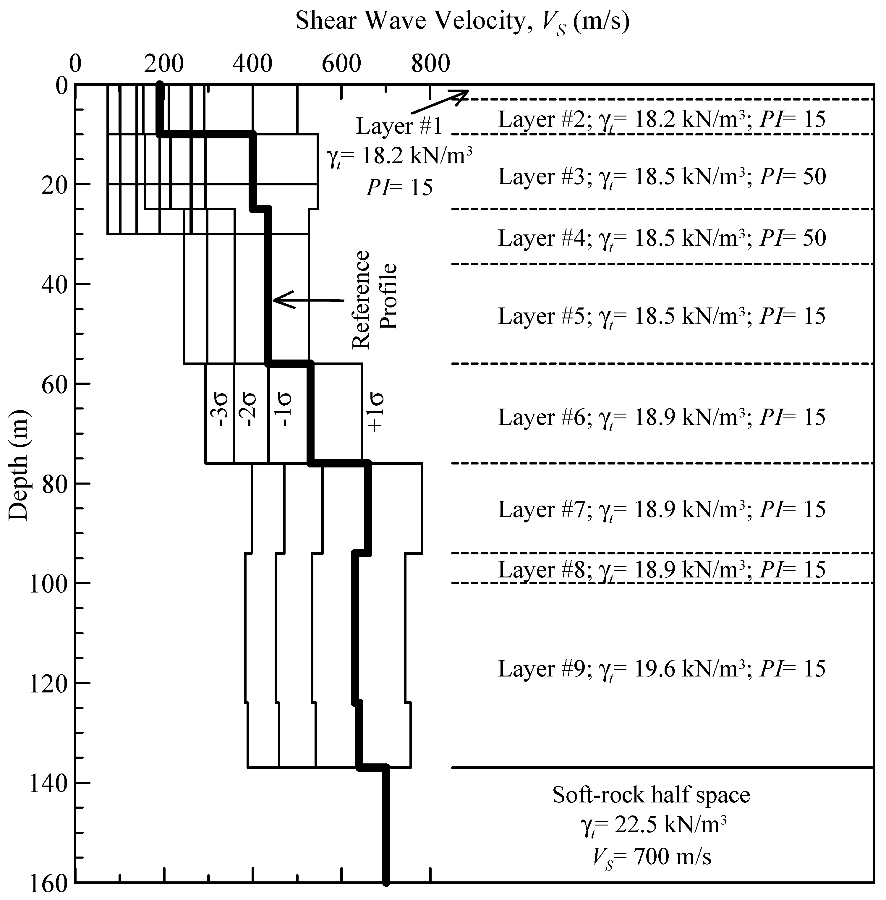
2.1. Geology and Dynamic Material Properties
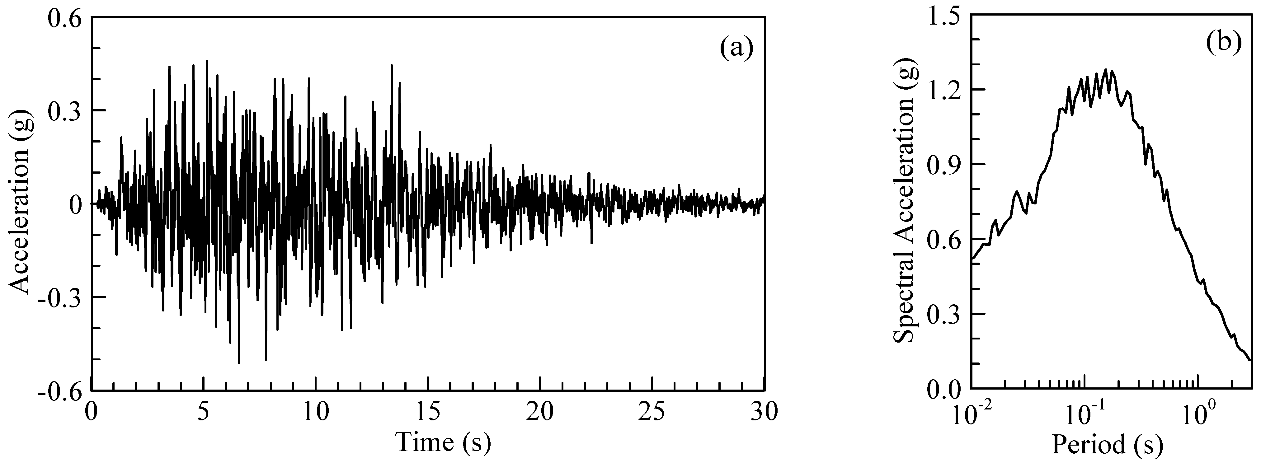
2.2. Seismology and Ground Motions
3. Site Response Analysis Software and Model Parameter Calibration
3.1. Equivalent Linear Site Response Analysis Using SHAKE2000
3.2. Nonlinear Site Response Analysis Using DMOD2000 and DEEPSOIL
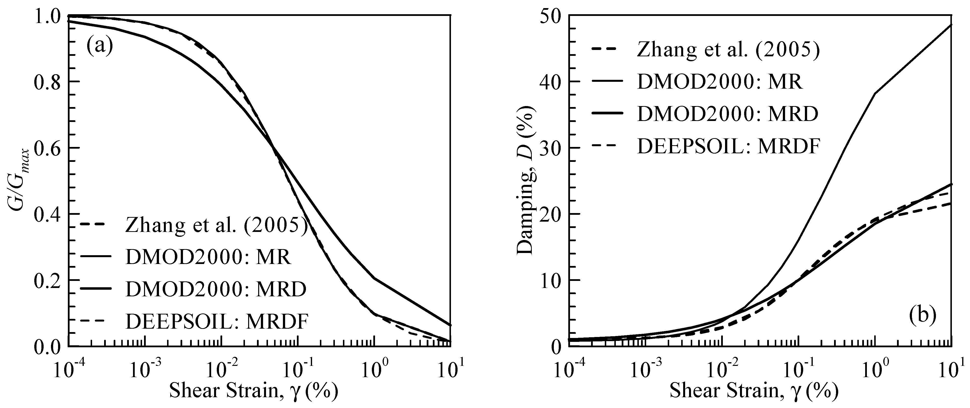
3.2.1. Constitutive Model and Shear Modulus Reduction
3.2.2. NNL Governing Equation and Viscus Damping Formulation
3.2.3. Hysteretic Damping Formulation
4. Analyses, Results, and Discussion
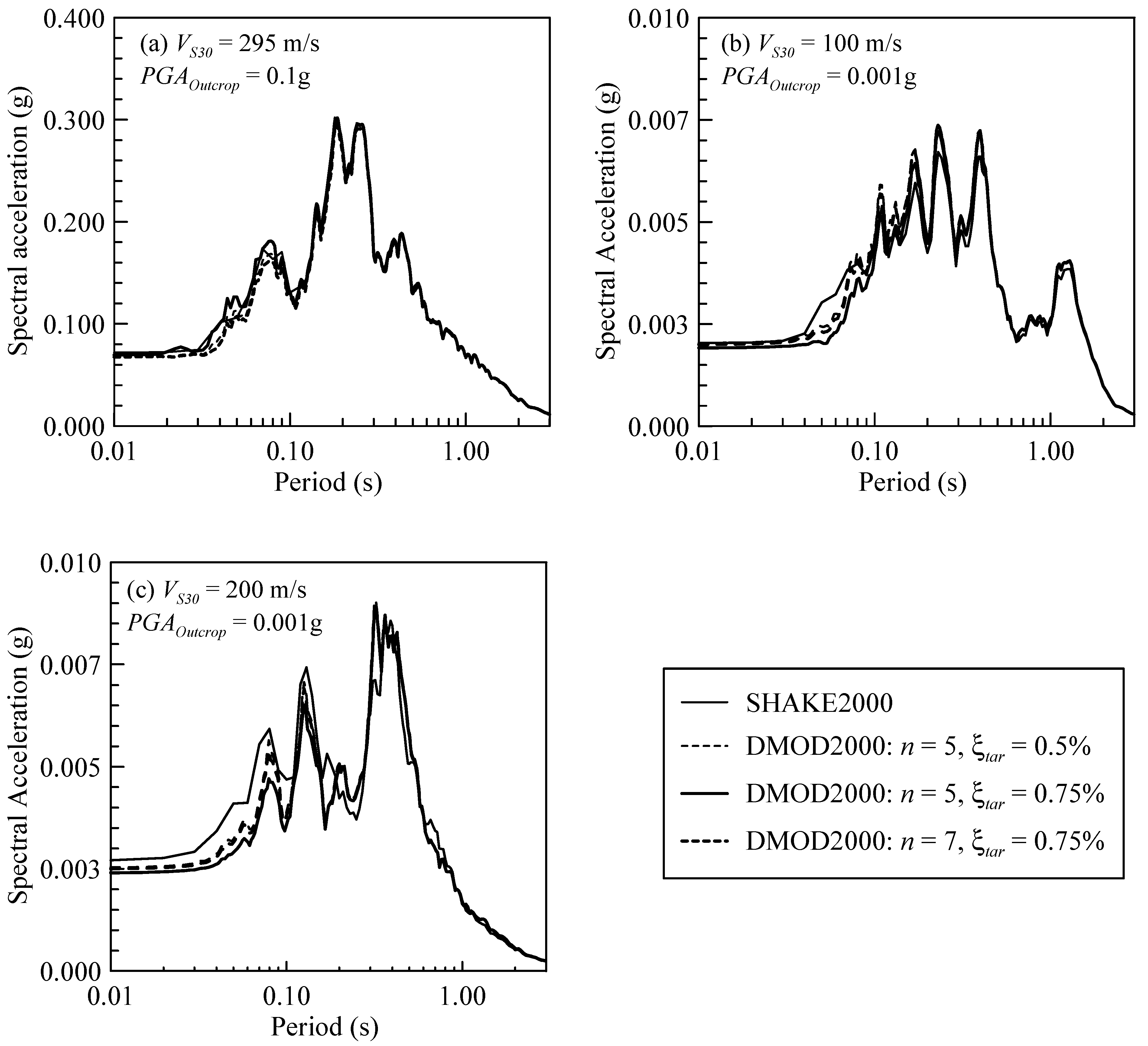
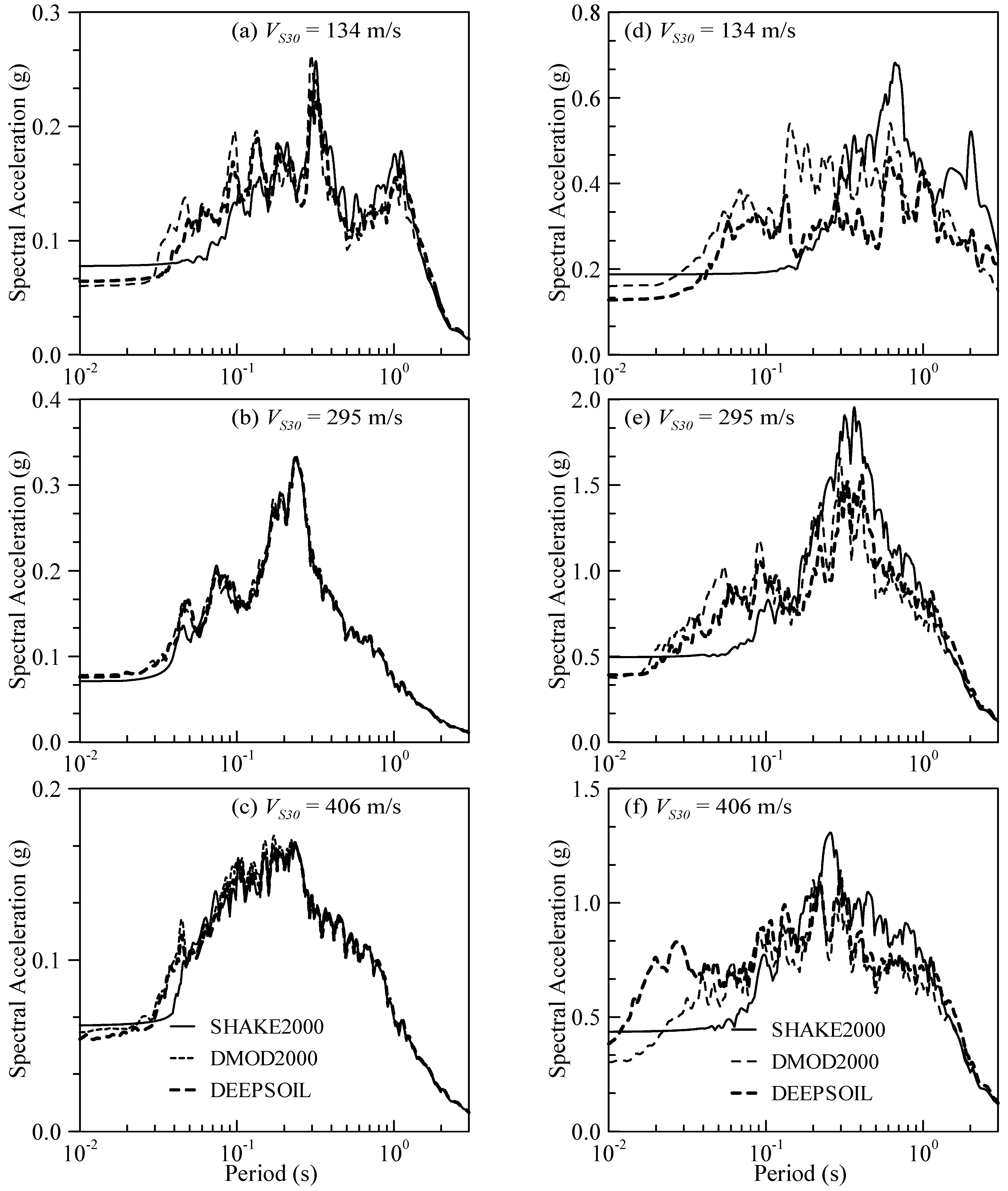
4.1. Comparison SHAKE2000, DMOD2000, and DEEPSOIL Results
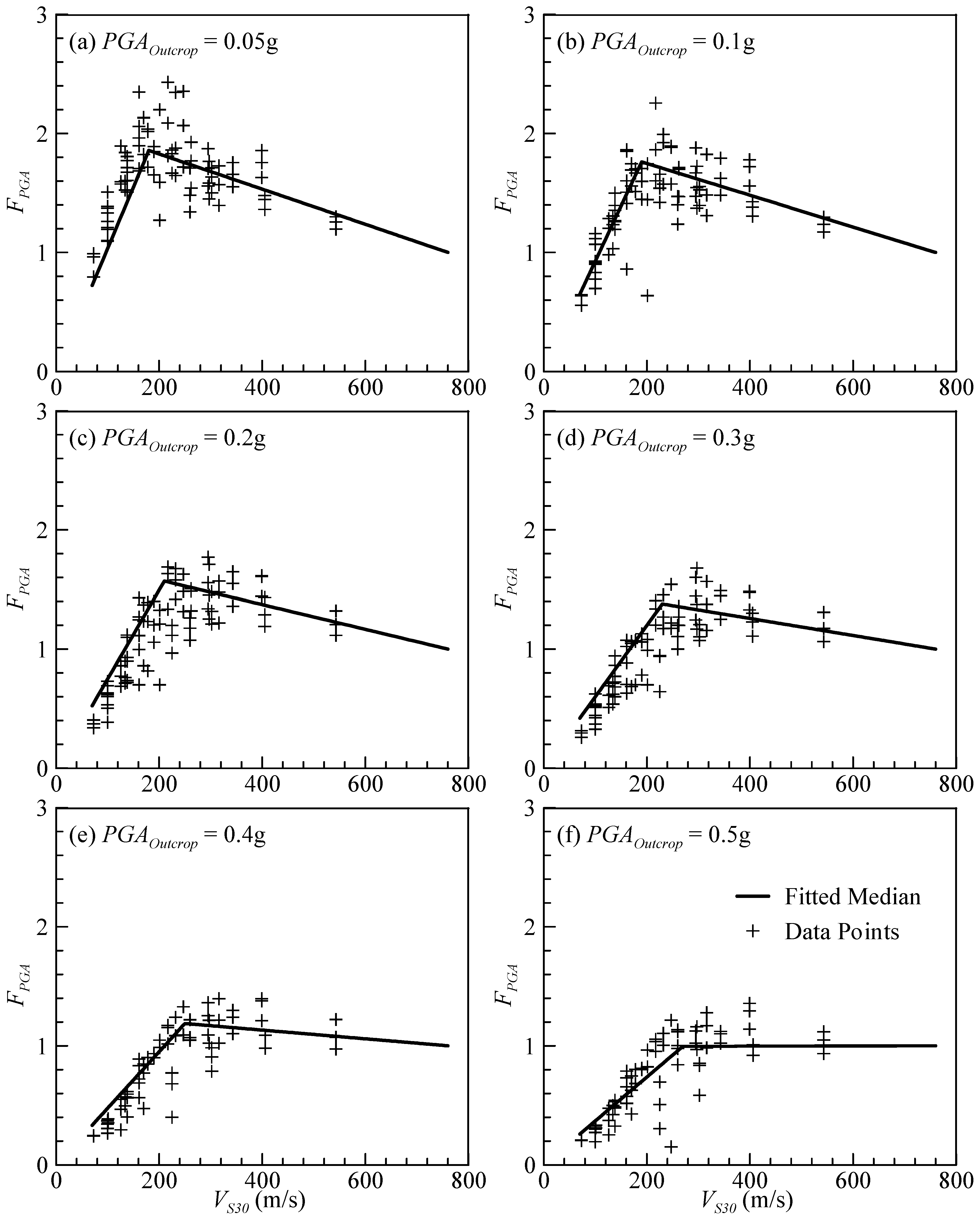
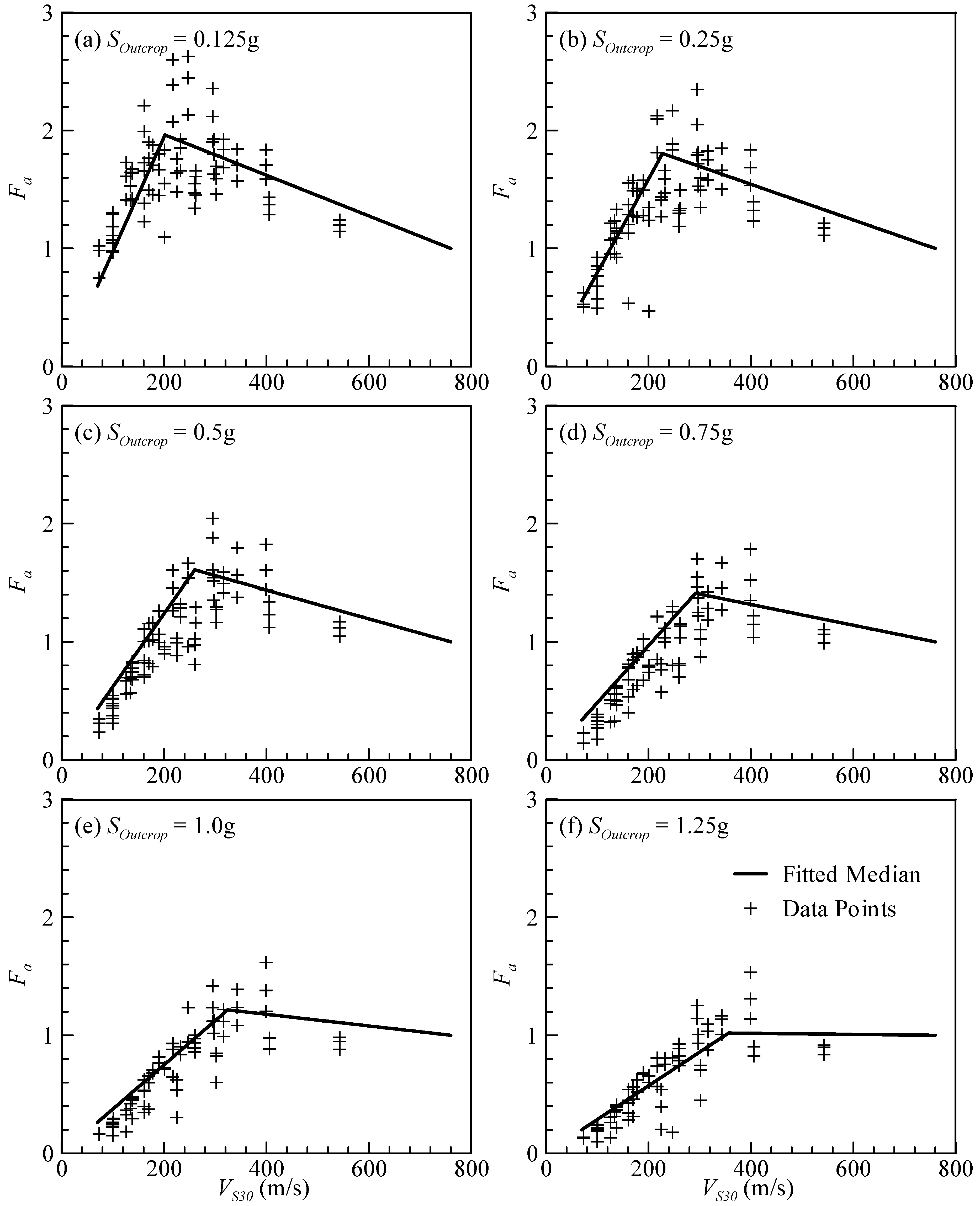
4.2. Development of Site Factor Models
4.3. Comparison of the Seismic Site Factor Models
4.4. Possible Reasons for the Difference Between Seismic Site Factor Models
4.5. Possible Reasons for the Difference Between DMOD2000 and DEEPSOIL Site Factor Models
5. Site Response Analysis Tool Selection Criterion—Threshold Chart
5.1. Key Steps
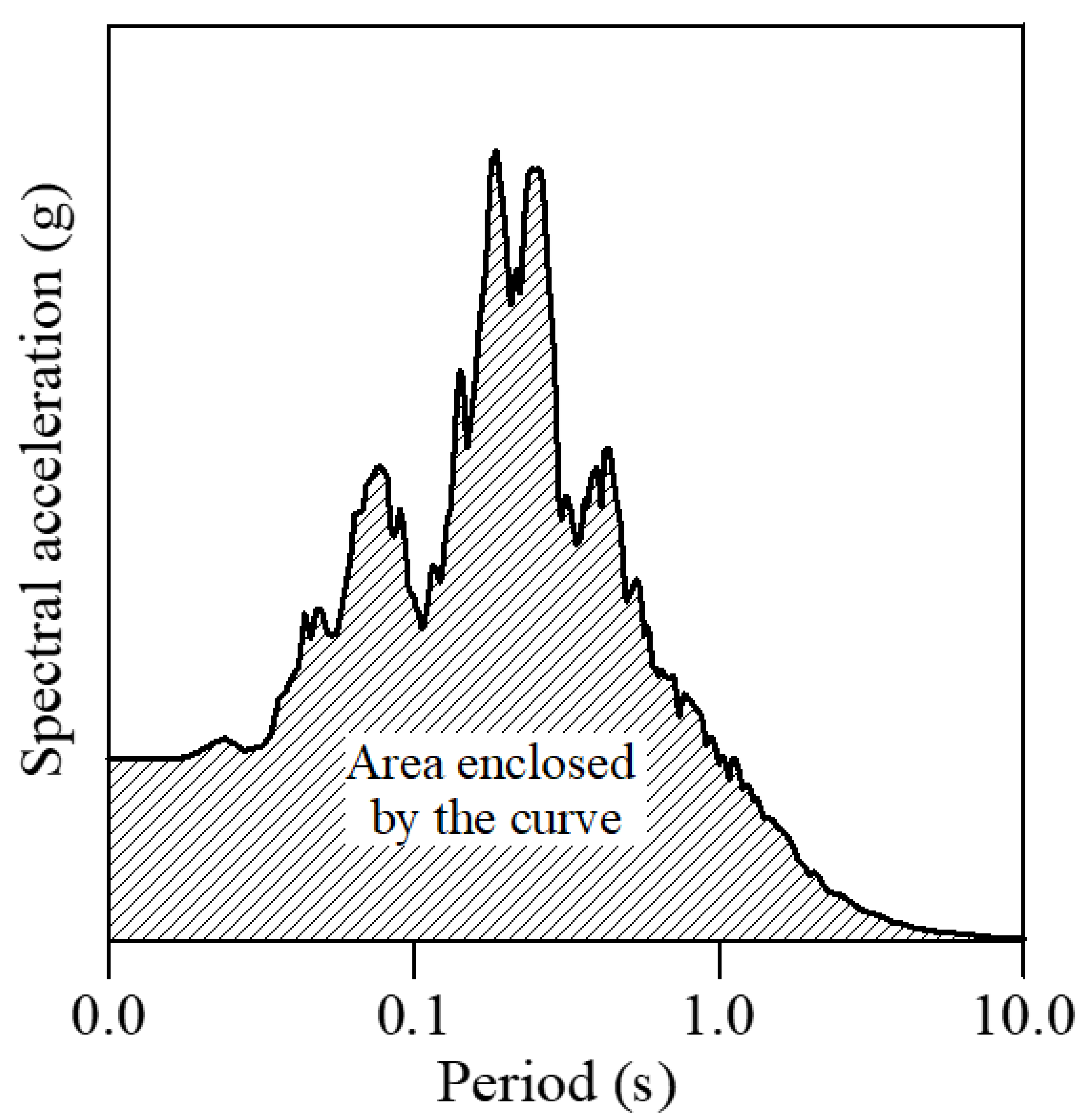
- (a)
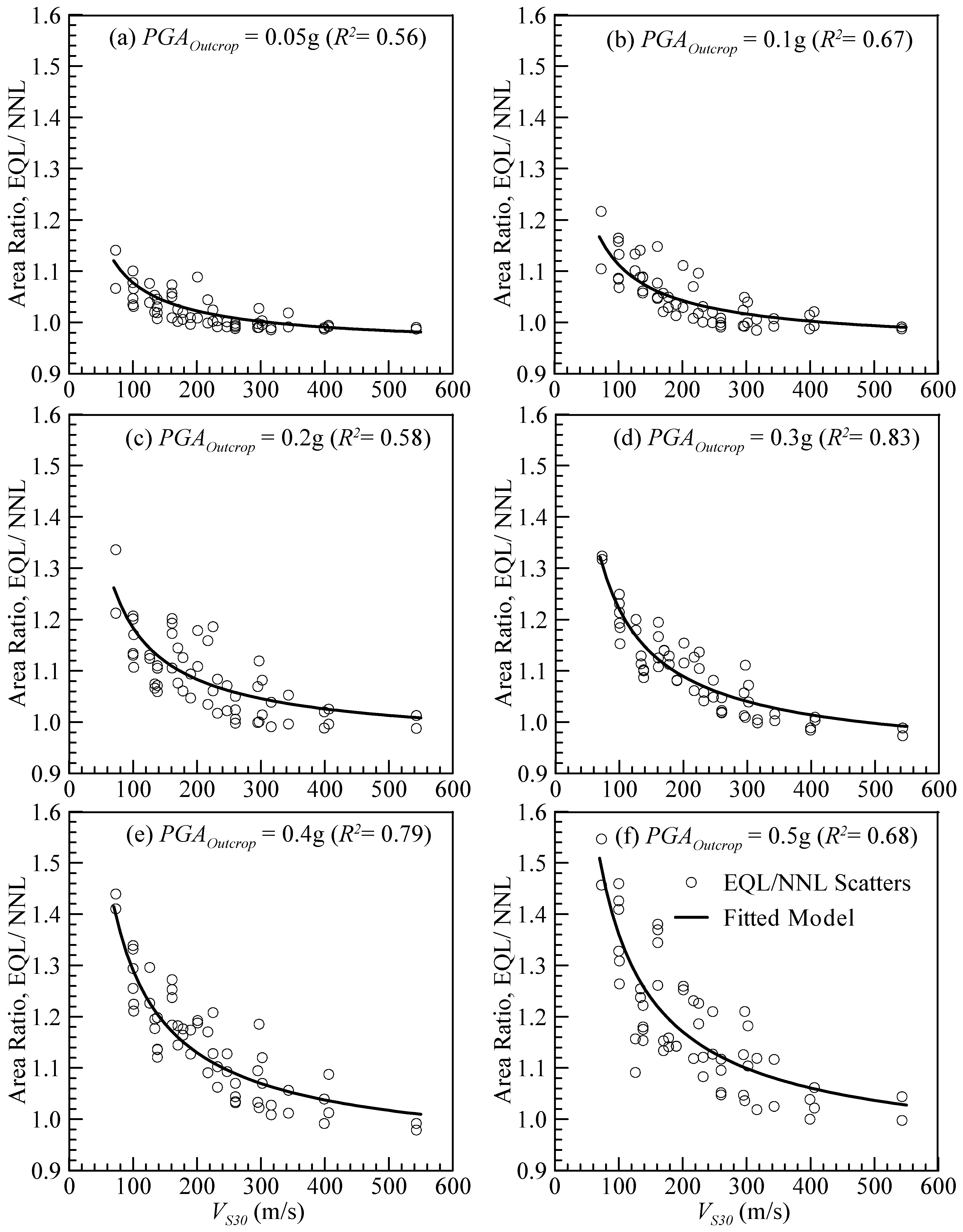
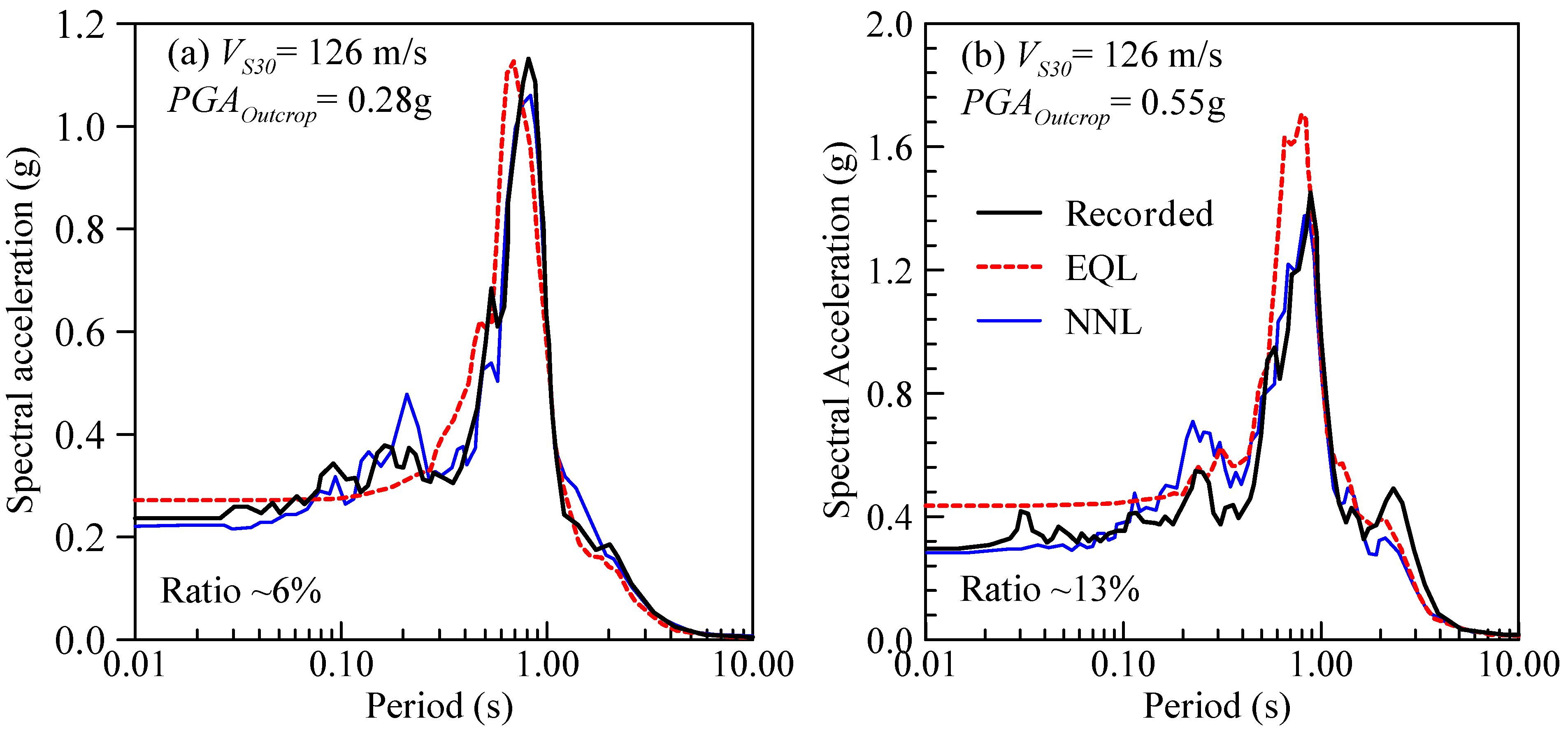
- The area under the surface response spectral acceleration plots between the period of 0.01 and 4.0 s, the shaded area shown in Figure 18, was calculated for each simulation result from each software.
- (b)
- For each of the VS30 cases, the arithmetic means of the area from all cases of ground motions were calculated from each simulation result for all six PGAOutcrop levels.
- (c)
- For each VS30, the corresponding averaged area ratios of SHAKE2000 to DMOD2000 and SHAKE2000 to DEEPSOIL were computed for all six PGAOutcrop levels.
- (d)
- The threshold chart, shown in Figure 19, was developed by considering VS30 and PGAOutcrop as the x- and y-axes, respectively. Then, the area ratios from SHAKE2000 to DMOD2000 and SHAKE2000 to DEEPSOIL were plotted using different markers for three distinct ranges identified: (a) less than 1.1 (10%), (b) between 1.1 to 1.2 (10 and 20%), and (c) greater than 1.2 (20%). Higher VS30 cases fall in the ’less than 10%’ range for PGAOutcrop values of up to 0.5 g.
5.2. Validations and Limitations
6. Conclusions
Author Contributions
Funding
Data Availability Statement
Acknowledgments
Conflicts of Interest
References
- Amevorku, C.; Andrus, R.D.; Rix, G.J.; Carlson, C.P.; Wong, I.G.; Ravichandran, N.; Jella, V.S.; Harman, N.E. Shear-wave velocity model of reference site conditions in South Carolina for site response analysis and probabilistic seismic hazard mapping. Eng. Geol. 2023, 323, 107200. [Google Scholar] [CrossRef]
- Sedaghat, A.; Amevorku, C.; Andrus, R.; Wong, I.; Rix, G.; Carlson, C.; Ravichandran, N.; Harman, N. Development of Shear-Wave Velocity Profiles for Computing Amplification Factors for Reference Outcrop to Local Site Conditions in South Carolina. In Proceedings of the Geo-Congress 2023, Los Angeles, CA, USA, 16–29 March 2023. [Google Scholar] [CrossRef]
- Jaume, S.C.; Cramer, C.; Moulton, D.E.; Levine, N.S. Earthquake Hazards on the Charleston Peninsula, South Carolina Based Upon ‘History-Informed’ Geological Mapping. In Proceedings of the Geological Society of America Abstracts with Programs, Montréal, QC, Canada, 25–28 October 2020; p. 52. [Google Scholar] [CrossRef]
- Sasanakul, I.; Gassman, S.; Ruttithivaphanich, P.; Dejphumee, S. Characterization of shear wave velocity profiles for South Carolina Coastal Plain. AIMS Geosci. 2019, 5, 303–324. [Google Scholar] [CrossRef]
- Chapman, M.C. User’s Guide to SCENARIO_PC and SCDOTSHAKE, Report to the South Carolina; Department of Transportation: Columbia, SC, USA, 2006. [Google Scholar]
- Jella, V.S.; Ravichandran, N.; Carlson, C.; Wong, I.; Rix, G.; Andrus, R.; Harman, N. Effects of Number of Spectral Periods and Input Motion Screening Criteria on the Representative Motions for Charleston, SC. In Proceedings of the Geo-Congress 2023, Los Angeles, CA, USA, 16–29 March 2023. [Google Scholar] [CrossRef]
- Matasovic, N.; Hashash YM, A. NCHRP428: Practices and Procedures for Site-Specific Evaluations of Earthquake Ground Motions (A Synthesis of Highway Practice); National Cooperative Highway Research Program, Transportation Research Board: Washington, DC, USA, 2012. [Google Scholar]
- Stewart, J.P.; Kwok, A.O.L.; Hashash, Y.M.A.; Matasovic, N.; Pyke, R.; Wang, Z.; Yang, Z. Benchmarking of Nonlinear Geotechnical Ground Response Analysis Procedures, Report PEER 2008/04; Pacific Earthquake Engineering Research Center, University of California: Berkeley, CA, USA, 2008. [Google Scholar]
- Kramer, S.L.; Paulsen, S.B. Practical Use of Geotechnical Site Response Models, in Proceedings International Workshop on Uncertainties in Nonlinear Soil Properties and their Impact on Modeling Dynamic Soil Response; University of California: Berkeley, CA, USA, 2004. [Google Scholar]
- Aboye:, S.A.; Andrus, R.D.; Ravichandran, N.; Bhuiyan, A.H.; Harman, N. Site factors for estimating peak ground acceleration in Charleston, South Carolina, based on VS30. In Proceedings of the 4th IASPEI/IAEE International Symposium: Effects of Surface Geology on Seismic Motion, Santa Barbara, CA, USA, 23–26 August 2011. [Google Scholar]
- Aboye, S.A.; Andrus, R.D.; Ravichandran, N.; Bhuiyan, A.H.; Harman, N. Seismic site factors and design response spectra based on conditions in Charleston, South Carolina. Earthq. Spectra 2013, 31, 723–744. [Google Scholar] [CrossRef]
- Tokimatsu, K.; Sugimoto, R. Strain-dependent soil properties estimated from downhole array recordings at Kashiwazaki-Kariwa nuclear power plant during the 2007 Niigata-ken Chuetsu-oki earthquake. In Proceedings of the Geotechnical Earthquake Engineering and Soil Dynamics IV, Sacramento, CA, USA, 18–22 May 2008; pp. 1–10. [Google Scholar] [CrossRef]
- Hartzell, S.; Bonilla, L.F.; Williams, R.A. Prediction of nonlinear soil effects. Bull. Seismol. Soc. Am. 2004, 94, 1609–1629. [Google Scholar] [CrossRef]
- Ardoino, F.; Traverso, C.M.; Parker, E.J. Evaluation of Site Response for Deepwater Field. In Proceedings of the Geotechnical Earthquake Engineering and Soil Dynamics IV, Sacramento, CA, USA, 18–22 May 2008; pp. 1–10. [Google Scholar] [CrossRef]
- Hashash, Y.M.; Phillips, C.; Groholski, D.R. Recent advances in nonlinear site response analysis. In Proceedings of the Fifth International Conference in Recent Advances in Geotechnical Earthquake Engineering and Soil Dynamics, San Diego, CA, USA, 24–29 May 2010. [Google Scholar]
- Kaklamanos, J.; Bradley, B.A.; Thompson, E.M.; Baise, L.G. Critical Parameters Affecting Bias and Variability in Site-Response Analyses Using KiK-net Downhole Array Data. Bull. Seismol. Soc. Am. 2013, 103, 1733–1749. [Google Scholar] [CrossRef]
- Kaklamanos, J.; Baise, L.G.; Thompson, E.M.; Dorfmann, L. Comparison of 1D linear, equivalent-linear, and nonlinear site response models at six KiK-net validation sites. Soil Dyn. Earthq. Eng. 2015, 69, 207–219. [Google Scholar] [CrossRef]
- Chapman, M.C.; Talwani, P. Seismic Hazard Mapping for Bridge and Highway Design, Report to the South Carolina; Department of Transportation: Columbia, SC, USA, 2002. [Google Scholar]
- Zhang, J.; Andrus, R.D.; Juang, C.H. Normalized shear modulus and material damping ratio relationships. J. Geotech. Geoenviron. Eng. 2005, 131, 453–464. [Google Scholar] [CrossRef]
- South Carolina Department of Transportation (SCDOT). Geotechnical Design Manual. Version 1.0; South Carolina Department of Transportation: Columbia, SC, USA, 2008.
- EPRI/DOE/NRC. Central and Eastern United States Seismic Source Characterization for Nuclear Facilities, NUREG-2115; EPRI/DOE/NRC: Palo Alto, CA, USA, 2012.
- Gheibi, E.; Gassman, S. Application of GMPEs to estimate the minimum magnitude and peak ground acceleration of prehistoric earthquakes at Hollywood, SC. Eng. Geol. 2016, 214, 60–66. [Google Scholar] [CrossRef]
- Talwani, P.; Schaeffer, W.T. Recurrence rates of large earthquakes in the South Carolina Coastal Plain based on paleoliquefaction data. J. Geophys. Res. Solid Earth 2001, 106, 6621–6642. [Google Scholar] [CrossRef]
- South Carolina Department of Natural Resources (SCDNR). Generalized Geologic Map of South Carolina; South Carolina Department of Natural Resources and South Carolina Geological Survey: Columbia, SC, USA, 2005.
- Assimaki, D.; Li, W. Site- and ground motion-dependent nonlinear effects in seismological model predictions. Soil Dyn. Earthq. Eng. 2012, 32, 143–151. [Google Scholar] [CrossRef]
- Akin, M.K.; Kramer, S.L.; Topal, T. Dynamic soil characterization and site response estimation for Erbaa, Tokat (Turkey). Nat. Hazards 2016, 82, 1833–1868. [Google Scholar] [CrossRef]
- Sana, H.; Nath, S.K.; Gujral, K.S. Site response analysis of Kashmir valley during the 8 October 2005 Kashmir earthquake Mw 7.6 using geotechnical dataset. Bull. Eng. Geol. Environ. 2018, 78, 2551–2563. [Google Scholar] [CrossRef]
- Debnath, R.; Saha, R.; Haldar, S.; Patra, S.K. Seismic site response analysis of Indo-Bangla railway site at Agartala incorporating site-specific dynamic soil properties. Bull. Eng. Geol. Environ. 2022, 81, 239. [Google Scholar] [CrossRef]
- Atkinson, G.M.; Boore, D.M. Ground motion relations for eastern North America. Bull. Seismol. Soc. Am. 1995, 85, 17–30. [Google Scholar] [CrossRef]
- Cornell, C.A. Engineering seismic risk analysis. Bull. Seismol. Soc. Am. 1968, 58, 1583–1606. [Google Scholar] [CrossRef]
- Park, D.; Dong, K.; Chang-Gyun, J.; Taehyo, P. Development of probabilistic seismic site coefficients of Korea. Soil Dyn. Earthq. Eng. 2012, 43, 247–260. [Google Scholar] [CrossRef]
- NUREG-0800; Standard Review Plan for the Review of Safety Analysis Reports for Nuclear Power Plants: Lwr Edition—Design of Structures, Components, Equipment, and Systems (Chapter 3, Section 3.7.1). U.S. Nuclear Regulatory Commission: Washington, DC, USA, 2014.
- ASCE 4-16; Seismic Analysis of Safety-Related Nuclear Structures. American Society of Civil Engineers: Reston, Virginia, 2016.
- Matasović, N.; Ordóñez, G.A. DMOD2000: A Computer program for seismic response analysis of horizontally layered soil deposits. In Earthfill Dams and Solid Waste Landfills, User’s Manual; Geomotions, LLC: Lacey, WA, USA, 2011; Available online: http://www.geomotions.com (accessed on 15 May 2015).
- Matasovic, N.; Vucetic, M. Cyclic Characterization of Liquefiable Sands. J. Geotech. Geoenviron. Eng. 1993, 119, 1805–1822. [Google Scholar] [CrossRef]
- Hashash YM, A. DEEPSOIL, User Manual and Tutorial; University of Illinois at Urbana-Champaign: Urbana, IL, USA, 2011. [Google Scholar]
- Matasovic, N.; Vucetic, M. Seismic Response of Horizontally Layered Soil Deposits, Report No. ENG 93-182; School of Engineering and Applied Science, University of California: Los Angeles, CA, USA, 1993. [Google Scholar]
- Hashash, Y.; Park, D. Nonlinear one-dimensional seismic ground motion propagation in the Mississippi embayment. Eng. Geol. 2001, 62, 185–206. [Google Scholar] [CrossRef]
- Hudson MA RT, I.N.; Idriss, I.M.; Beikae, M. User’s Manual for QUAD4M. Center for Geotechnical Modeling; Department of Civil & Environmental Engineering, University of California: Davis, CA, USA, 1994. [Google Scholar]
- Phillips, C.; Hashash, Y.M.A. Damping formulation for nonlinear 1D site response analyses. Soil Dyn. Earthq. Eng. 2009, 29, 1143–1158. [Google Scholar] [CrossRef]
- Régnier, J.; Bonilla, L.F.; Bard, P.Y.; Bertrand, E.; Hollender, F.; Kawase, H.; Verrucci, L. PRENOLIN: International benchmark on 1D nonlinear site-response analysis—Validation phase exercise. Bull. Seismol. Soc. Am. 2018, 108, 876–900. [Google Scholar] [CrossRef]
- Kim, B.; Hashash, Y.M.; Kottke, A.R.; Assimaki, D.; Li, W.; Rathje, E.M.; Campbell, K.W.; Silva, W.J.; Stewart, J.P. A predictive model for the relative differences between nonlinear and equivalent-linear site response analyses. In Proceedings of the 22nd International Conference in Structural Mechanics in Reactor Technology, San Francisco, CA, USA, 18–23 August 2013. [Google Scholar]
- Afacan, K.B.; Brandenberg, S.J.; Stewart, J.P. Centrifuge modeling studies of site response in soft clay over wide strain range. J. Geotech. Geoenviron. Eng. 2013, 140, 04013003. [Google Scholar] [CrossRef]
- Brandenberg, S.J.; Stewart, J.P.; Afacan, K. Influence of Liquefaction on Earthquake Ground Motions; Final Report for USGS, Award Number G12AP20098; USGS: Asheville, NC, USA, 2013.


| Regression Coefficients * | ||||||
|---|---|---|---|---|---|---|
| Spectral Period, T (s) | SOutcrop | x1 (g−1) | x2 | x3 (g−1·m/s) | x4 (m/s) | a |
| 0.0 | PGAOutcrop | −1.91, −1.39, −1.40 | 1.95, 1.62, 1.27 | 200, 270, 270 | 170, 174, 174 | - |
| 0.2 | Ss | −0.79, −0.76, −0.61 | 2.00, 1.97, 1.48 | 129, 84, 84 | 195, 207, 207 | 0.65 |
| 0.6 | S0.6 | −2.26, −2.52, −2.92 | 2.86, 2.68, 2.71 | 207, 139, 156 | 156, 183, 182 | 0.85 |
| 1.0 | S1 | −2.39, −2.50, −3.40 | 3.43, 2.89, 3.41 | 129, 124, 97 | 153, 147, 156 | 0.90 |
| 1.6 | S1.6 | −4.46, −4.92, −4.92 | 3.49, 3.22, 3.21 | 198, 323, 324 | 121, 113, 133 | 0.97 |
| 3.0 | S3.0 | −8.2, −4.389, −0.97 | 2.80, 2.10, 2.21 | 394, 346, 482 | 80, 85, 131 | 0.99 |
Disclaimer/Publisher’s Note: The statements, opinions and data contained in all publications are solely those of the individual author(s) and contributor(s) and not of MDPI and/or the editor(s). MDPI and/or the editor(s) disclaim responsibility for any injury to people or property resulting from any ideas, methods, instructions or products referred to in the content. |
© 2025 by the authors. Licensee MDPI, Basel, Switzerland. This article is an open access article distributed under the terms and conditions of the Creative Commons Attribution (CC BY) license (https://creativecommons.org/licenses/by/4.0/).
Share and Cite
Ravichandran, N.; Bhuiyan, M.A.H.; Jella, V.S.; Bahuguna, A.; Sundararajan, J. Comparison of Seismic Site Factor Models Based on Equivalent Linear and Nonlinear Analyses and Correction Factors for Updating Equivalent Linear Results for Charleston, South Carolina. Geosciences 2025, 15, 115. https://doi.org/10.3390/geosciences15040115
Ravichandran N, Bhuiyan MAH, Jella VS, Bahuguna A, Sundararajan J. Comparison of Seismic Site Factor Models Based on Equivalent Linear and Nonlinear Analyses and Correction Factors for Updating Equivalent Linear Results for Charleston, South Carolina. Geosciences. 2025; 15(4):115. https://doi.org/10.3390/geosciences15040115
Chicago/Turabian StyleRavichandran, Nadarajah, Md. Ariful H. Bhuiyan, Vishnu Saketh Jella, Ashish Bahuguna, and Jatheesan Sundararajan. 2025. "Comparison of Seismic Site Factor Models Based on Equivalent Linear and Nonlinear Analyses and Correction Factors for Updating Equivalent Linear Results for Charleston, South Carolina" Geosciences 15, no. 4: 115. https://doi.org/10.3390/geosciences15040115
APA StyleRavichandran, N., Bhuiyan, M. A. H., Jella, V. S., Bahuguna, A., & Sundararajan, J. (2025). Comparison of Seismic Site Factor Models Based on Equivalent Linear and Nonlinear Analyses and Correction Factors for Updating Equivalent Linear Results for Charleston, South Carolina. Geosciences, 15(4), 115. https://doi.org/10.3390/geosciences15040115