Abstract
A magnitude (M) 7.7 quake struck on 6 February 2023 in Turkey. Nine hours later, a M7.5 quake occurred near the initial M7.7 quake. We studied seismicity before and after these doublet quakes, integrating physics-based and statistical approaches. We first used the statistical Epidemic-Type Aftershock Sequence (ETAS) and the Bayesian Gutenberg–Richter b-value models to confirm previously reported seismicity transients (seismic activation and low b values) prior to the future M7.7 quake. We then showed that the low b-value area coincided with a high-slip area on the strand segment from which the M7.7 rupture started, a similar result to that obtained for the 2011 Tohoku megaquake case in Japan. We next used the physics-based Coulomb and statistical b-value models to find that the locations of the largest and second-largest events in the post-doublet-quake sequence were in relatively high-stress regions and became closer to failure as a result of the doublet quakes. We further used the ETAS model to show that this sequence is currently active but is decaying with time. The duration of the sequence was estimated at 2.7–5.5 years, which is longer than previously proposed (1–2.5 years). Our result was stable because it was based on quake data from about 600 days, six times longer than the study period used in a previous study.
1. Introduction
On 6 February 2023 (UTC), a devastating quake of magnitude (M) 7.7 struck the East Anatolian fault zone (EAFZ) that bounds the Anatolian and Arabian plates (Figure 1a). This quake, which occurred near the city of Kahramanmaraş in Turkey, was followed about nine hours later by a M7.5 quake approximately 90 km to the north of the initial M7.7 quake.
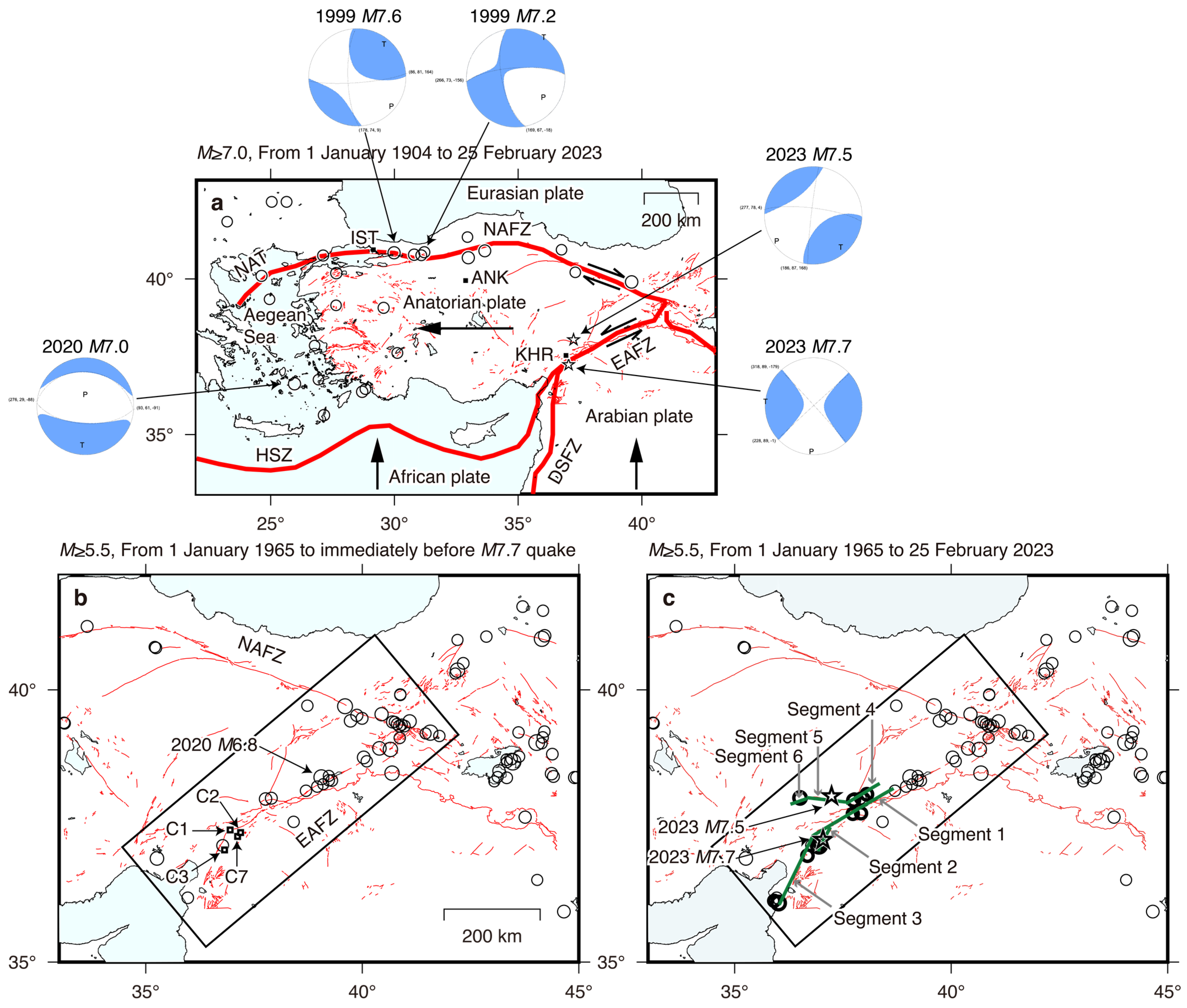
The seismicity in Turkey is attributed to the relative motions of the Arabian, Eurasian, African, and Anatolian plates. Thick black arrows in Figure 1a schematically indicate the motion of the Arabian, African, and Anatolian plates [1]. Thick red curves indicate plate boundaries. The North Anatolian fault zone (NAFZ), Hellenic subduction zone (HSZ), North Aegean Trough (NAF), and EAFZ are the major tectonic structures of this Anatolia–Aegean region. Seismically active areas based on M ≥ 7 quakes (Figure 1a) are along the NAFZ and EAFZ, in the western part of Turkey where active faults (thin red curves) are densely distributed, and in the Aegean Sea. The five most recent quakes of M ≥ 7, including the doublet quakes (the M7.7 and 7.5 quakes), are highlighted by showing the focal mechanism for each of these five quakes. The crustal deformation associated with the doublet quakes can be treated as shear deformation (half-arrow pair) across the EAFZ, accommodating the westward movement of Turkey into the Aegean Sea. The broad context of the doublet quakes is that they occurred under the current tectonic stress that created the EAFZ. While the relative plate motions in the region around the EAFZ are low (typically less than 10 mm/yr), even regions with slow plate motions can host extremely damaging quakes [1].
As described in the next section detailing the research area background [2,3,4,5,6,7,8,9,10,11,12,13,14,15,16,17], the characteristics of seismic activity before and after the doublet quakes provide reference values to act as a basis for predictions of the seismic hazards of regional strong earthquakes around the EAFZ. However, to our knowledge, strengthening the robustness of previous findings has not been fully addressed based on currently observable data. The purpose of this study is to address this issue, integrating statistical and physics-based approaches, and to put forward some new views on pre- and post-doublet-quake sequences.

Figure 1.
Seismicity in and around the doublet quakes. (a) Thin circles indicate the epicenters of quakes with M ≥ 7.0 with a depth of 40 km or shallower during the period from 1 January 1904 to 25 February 2023, where the combined catalog was used (see the Data Section). Stars indicate the M7.7 and 7.5 epicenters. The beach ball indicates the focal mechanism for each of the five recent quakes. Thick red curves indicate the plate boundaries. Large arrows schematically indicate plate motion. Thin red curves indicate active faults. NAFZ, EAFZ, HSZ, DSFZ, NAT, IST, ANK, and KHR indicate the North and East Anatolian fault zones, the Hellenic subduction zone, the Dead Sea fault zone, the cities of Istanbul, Ankara, and Kahramanmaraş, respectively. The half-arrow pair indicates the relative motion across the NAFZ and EAFZ. (b) Thin circles indicate quakes with M ≥ 5.5 with a depth of 40 km or shallower during the period from 1 January 1965 to immediately before the 2023 M7.7 quake. Quakes in the rectangular region are considered in the Discussion Section. Open squares indicate the locations of clusters C1, C2, C3, and C7 [10]. (c) Thin circles are the same as those in (b). Thick circles are the same as thin ones for the period after the M7.7 quake. Green lines show the M7.7 and 7.5 source faults [2,3]. Fault segments are numbered 1 to 6 (see the Data Section). Segment 2 indicates the location and scope of the cross-section in Section 5.1.3.
2. Research Area Background
The NAFZ ruptured in a series of M ≥ 7 quakes during the twentieth century [1] (Figure 1a). During the same period, the EAFZ experienced M6 quakes, with most of the seismic activity on the northern section. Seismic activity on the southern section of the EAFZ started with the 24 January 2020 M6.8 quake (Figure 1b). Figure 1c shows how the remainder of the southern section was activated during the 2023 doublet quakes and following events, where seismicity (M ≥ 5.5) from 1965 to the M7.7 quake (thin circles) is overlaid with seismicity after the M7.7 quake (thick circles) and fault segments of the doublet quakes (green) [2,3].
The focal mechanism of the 2020 M6.8 quake indicates faulting on a near-vertical left-lateral plane trending SW-NE [4]. A slip on this plane is generally consistent with local plate motions and the orientation of regional faults. The M7.7 quake involved a left-lateral strike-slip along SW-NE-trending faults [2]. A predominant mechanism of the M7.5 quake was a left-lateral strike-slip fault motion along SW-NE- and E-W-trending faults [3].
The preceding M7.7 quake promoted the subsequent M7.5 quake, largely by unclamping stress loaded on the epicentral patch of the future rupture [5]. Chen et al. [6] also showed that the M7.5 quake was promoted by historical quakes and finally triggered by the M7.7 quake. As performed in several studies [5,6,7,8,9], it is of interest to analyze the interaction between the doublet quakes. However, this possibility is beyond the scope of the present study. Rather, we focused on seismicity before and after the doublet quakes.
Kwiatek et al. [10] reported seismicity transients starting approximately 8 months before the 2023 M7.7 quake. One of the main characteristics of the transients was seismic activation (see also [11]). Seismicity was composed of isolated spatiotemporal clusters near the future M7.7 epicenter. Four clusters were recognized within 50 km of the future epicenter, referred to as C1, C2, C3, and C7 [10] (Figure 1b). Clusters C1 and C2 emerged within 8 months prior to the M7.7 quake. Clusters C2 and C7 were located on and around a fault segment (segment 2 defined in the Data Section) where the M7.7 quake initiated. Cluster C7 emerged in 2017–2018. Cluster C3 was activated in 2015, 2016, and 2021. The other main characteristic was the low b value of the Gutenberg–Richter (GR) frequency–magnitude relation of quakes [12]. This relation will be defined in the Methods Section. Clusters C1 and C2 were responsible for the low b values [10]. The authors in [10] also showed non-Poissonian inter-event time statistics and magnitude correlations of seismicity.
Seismicity after the doublet quakes was still active. About 4500 M ≥ 3 quakes occurred around the causative faults during the period since the M7.7 quake until 16 October 2024, when we used the Disaster and Emergency Management Authority (AFAD) catalog (see the Data Section). Two M6-class quakes occurred after the doublet quakes: an M6.4 quake on 20 February. 2023 [13] and an M5.9 quake on 16 October 2024 [14] around the south and north ends of the M7.7 rupture, respectively. Given that the fault end zones generally calculate increases in stress [7], the areas surrounding these M6-class quakes were hypothesized to be heading toward failure using the stress calculation. In the present study, this hypothesis was supported by using currently available quake data and fault models.
Although active seismicity continues, the post-doublet-quake sequence undergoes the Omori–Utsu (OU) power-law decay over time [15] (see the Methods Section). Toda and Stein [5] estimated the duration of the post-doublet-quake sequence to be 1–2.5 years. This duration was defined as the period during which the occurrence rate computed using the OU relation was larger than that of ordinary quakes before the 2020 M6.8 quake. Re-evaluation of the duration of this sequence would provide the basis of a time-dependent seismic hazard assessment along the EAFZ, because almost 1.5 years have passed since the M7.7 quake (as of October 2024).
As pointed out in the Introduction Section, we verified some previous views described above and put forward some new views of seismicity along the EAFZ. For this purpose, we studied seismicity before and after the doublet quakes using earthquake catalogs created by the AFAD, Lomax [16], and Kwiatek et al. [10] to demonstrate that the result does not depend on the choice of catalog. In Section 5.1, we confirmed previously reported seismicity transients during the pre-doublet-quake sequence [10] using the statistical Epidemic-Type Aftershock Sequence (ETAS [17]) and GR models. Taking both physics-based and statistical approaches, we investigated the post-doublet-quake sequence, which indicated that the two M6-class quakes were promoted by the doublet quakes (Section 5.2), and we discuss a comparison in the duration of this sequence between our study and a previous study [5] in Section 6.
3. Methods
3.1. OU Relation and ETAS Model
Seismicity after a large quake is often correlated with the OU relation [15] in the time domain, given as λOU = k(c + t)−p, where λOU is the number of quakes per unit time at t with M larger than or equal to a minimum threshold magnitude (Mth), and p, c, and k are positive constants. The OU relation with p = 1 is assumed as a standard form according to the rate- and state-dependent friction law [18]. Variability in p is the possibility p < 1 and p > 1 for special cases with slowly and rapidly decreasing stress, respectively. The ETAS model described below considers a quake sequence as a result of the onset of the OU power-law decay following each previous event.
In the framework of the ETAS model [17], all quakes are decomposed into Poisson background activity and clustering activity. To express the clustering activity, each quake is assumed to be followed by quakes in the form of the OU relation. The rate of quake occurrence at t following the i-th quake with magnitude Mi (≥Mth) and time ti (<t) is given by νi(t) = Ω(t − ti + c)-p, where Ω = K0exp{α(Mi − Mth)}, and K0 and α are positive constants.
The occurrence rate of the whole quake series at t becomes , where μ is a positive constant, the summation is performed for all i satisfying ti < t, S is the starting time for the analysis, and Ht represents the history of occurrence times with associated magnitudes from the data {(ti, Mi)} before t. The first and second terms of the right-hand side of the equation represent the occurrence rates of the Poisson background activity and the clustering activity, respectively. The parameter set θ = (μ, K0, α, c, p) represents the characteristics of whole seismic activity. The unit of μ (first term) is day−1. The units of the remaining parameters in the second term are day−1, no unit, day, and no unit for K0, α, c, and p, respectively. We used the Akaike Information Criterion (AIC) [19] that is useful to assess the goodness-of-fit between the model and data and is obtained from the number of adjusted parameters and the maximum log-likelihood.
How well (or poorly) the ETAS model fits a quake sequence is able to be visualized by comparing the rate calculated by the model and the cumulative number of quakes [20]. One can visualize this comparison in two types of graphs: one graph using ordinary time and the other using transformed time. Here, transformed time is converted from ordinary time in such a way that the transformed sequence follows the Poisson process (uniformly distributed occurrence times) with unit intensity (occurrence rate). When a good approximation of observed seismicity is presented by the model, one sees an overlap between the observation rate and model rate in both types of graphs.
3.2. GR Relation
The GR relation [12] is given by log10N = a − bM, where N is the number of quakes with a magnitude ≥ M, and a is a constant. A constant b is used to describe the relative occurrence of small and large quakes (i.e., a low b value indicates a smaller proportion of small quakes, and vice versa) [21,22,23,24,25]. The b value is calculated based on quakes with a magnitude above Mc called the completeness magnitude, above which a seismic network is considered to detect all quakes.
A systematic decrease in the b value approaching the time of the entire fracture was indicated by the results of laboratory experiments [26,27,28]. In this context, for the period leading up to large-size quakes in Sumatra, Japan, and Chile [28,29,30,31], there were reports of low b values and/or a decrease in b. However, it remains unclear whether underlying physical processes associate with the time-dependent changes in b, and the role of b as a stress meter is unproven. Nonetheless, laboratory experiments [26] and numerical simulations [32] indicated such processes and the role of b. One possible physical model showed that an increased stress level in slowly slipping parts of a fault facilitates quake rupture growth, resulting in the temporal decrease in b prior to a large quake (mainshock) [32]. Another possible model showed that the decrease in b is caused by a rapid increase in shear stress, promoting micro-crack growth [26].
3.3. Stress Change Calculation
Coulomb software (version 3.3) [33,34] was used to calculate how quakes promote or inhibit failure of nearby faults. Static stress changes caused by the displacement of a fault (source fault) were calculated. Displacements in the elastic half-space were used to calculate the 3D strain field; this was multiplied by elastic stiffness to derive the stress changes. Typical values for the friction coefficient (μ = 0.4), Young’s modulus (E = 8 × 10⁵ bar), and Poisson’s ratio (PR = 0.25) were used in this study. The resulting shear modulus (G = E/[2(1 + PR)] = 3.3 × 10⁵ bar) was also used. The normal and shear components of the stress change were resolved on specified receiver fault planes. A receiver fault consists of planes, each characterized by a specified strike, dip, and rake, on which the stresses imparted by the source faults are resolved. The Coulomb failure criterion, in which failure is inhibited (promoted) when the Coulomb failure is negative (positive), was used.
4. Data
4.1. Quake Catalogs
For analyses of long-term seismicity (Figure 1), we created a quake catalog based on the ISC-GEM catalog (version 9.1, released on 27 June 2022) [35,36,37,38] and the ANSS catalog [39]. The catalog we created contains quakes with M ≥ 5.5 during the period 1 January 1904–31 December 2018 obtained from the ISC-GEM catalog and during the period 1 January 2019–25 February 2023 obtained from the ANSS catalog.
For analyses of short-term seismicity, we used three quake catalogs created by the AFAD, Lomax [16], and Kwiatek et al. [10] to demonstrate that the result does not depend on the choice of catalog. We downloaded the AFAD catalog, including quakes of M ≥ 1.0 from 1 January 2014 to 16 October 2024. This timing of 1 January 2014 coincided with the start of the improved generation of the local seismicity catalog by the AFAD [10]. Although we filtered out events specified as explosion, downthrow, volcanic, and unknown when downloading the catalog, it is known that it includes clusters corresponding to quarry-blast activity [10]. In this study, the events located within areas of the quarry-blast shown in Kwiatek et al. [10] were excluded from the catalog. According to Kwiatek et al. [10], the AFAD catalog has Mc = 1.5 within a 50 km radius from the M7.7 quake during a period from 1 January 2023 to immediately before the M7.7 quake (6 February 2023).
The Lomax catalog [16] (version 3.0, released on 28 January 2023), which includes quakes from 1 January to 31 May 2023, is an NLL-SSST-coherence hypocenter catalog, where NLL-SSST-coherence [40,41] is an enhanced, absolute-timing quake location procedure that (1) iteratively generates spatially varying travel time corrections to improve multi-scale location precision, and (2) uses waveform similarity to improve fine-scale location precision. Lomax [16] performed relocations with merged phase arrival data available from the Kandilli Observatory and Earthquake Research Institute (KOERI) and the AFAD. This author used all events in the AFAD catalog with M ≥ 1.5 for relocation.
Kwiatek et al. [10] produced a seismicity catalog around the M7.7 and 7.5 quakes for a period from 1 January 2023 to immediately before the M7.7 quake (6 February 2023). This catalog was generated by using an AI-based workflow [10]. When the events located within areas identified as quarry-blasts were excluded, only events representing quakes remained. The catalog has Mc = 0.5 in the 50 km radius around the M7.7 epicenter [10].
4.2. Fault Models
The fault model of the M7.7 quake is based on the work by the United States Geological Survey (USGS) [2]. This is a finite-fault model with numerous small patches of slips, each having information on the location of a rectangular patch, strike, dip, and rake. The model that includes analysis of both teleseismic and regional seismic and geodetic observations represents three plane segments (1, 2, and 3) showing two main ruptures on segments 1 and 3 with one strand (segment 2) near the M7.7 hypocenter (Figure 1c). The fault geometry has a length of 185 km and width of 39 km with strike/dip/rake = 60°/85°/3° for segment 1, a length of 50 km and width of 40 km with 28°/85°/0° for segment 2, and a length of 155 km and width of 38 km with 25°/75°/−3° for segment 3. Considering the location of the M7.7 hypocenter, the rupture initiated on segment 2, and the rupture radiation was bilateral along segments 1 and 3. This is consistent with the rupture model of the M7.7 quake [42]. A slip distribution for the rupture along segments 1 and 3 shows peak-slip values of >10 m, but along segment 2 it shows peak-slip values of about 1.5 m. The model representing the three segments involves predominantly near-vertical left-lateral strike-slip faulting.
The finite-fault model of the M7.5 quake, based on work by the USGS [3], was used. This model that represents three segments (4, 5, and 6) involves predominantly near-vertical left-lateral strike-slip faulting. The fault geometry has a length of 75 km and width of 30 km with strike/dip/rake = 60°/80°/3° for segment 4, a length of 75 km and width of 30 km with 276°/80°/−12° for segment 5, and a length of 30 km and width of 30 km with 250°/80°/16° for segment 6. Considering the location of the M7.5 hypocenter, the rupture initiated on central segment 5, and the rupture radiation was bilateral along two segments (4 and 6) located at both ends of segment 5, consistent with the rupture model of the M7.5 quake [42]. A slip distribution for the rupture along segment 5 shows peak-slip values of >10 m, while along segments 4 and 6 it shows peak-slip values < 10 m.
To calculate how the doublet quakes promoted or inhibited the M6.4 quake, a moment tensor solution of the M6.4 quake reported by the USGS [13] was used. The moment tensor contains two nodal planes (NPs). Both NPs were used as receiver faults of changes in Coulomb stress imparted by the doublet quakes. Similarly, a moment tensor solution of the M5.9 quake reported by the USGS [14] was used.
In this study, we used the USGS moment tensor solutions because we used the USGS fault models of the M7.7. and 7.5 quakes [2,3] and considered consistency of the source between the moment tensor solutions and the fault models. Our future research requires the use of the moment tensor solutions of not only the USGS but also from other sources to strengthen the robustness of our findings. Examples include the moment tensor solutions reported by the KOERI at http://www.koeri.boun.edu.tr/sismo/2/moment-tensor-solutions/ (accessed on 17 March 2025) and by the GFZ Helmholtz Centre for Geosciences at https://geofon.gfz.de/old/eqinfo/eqinfo.php (accessed on 17 March 2025).
5. Results
5.1. Pre-Doublet-Quake Sequence
5.1.1. b Value and Change in Seismicity Rate
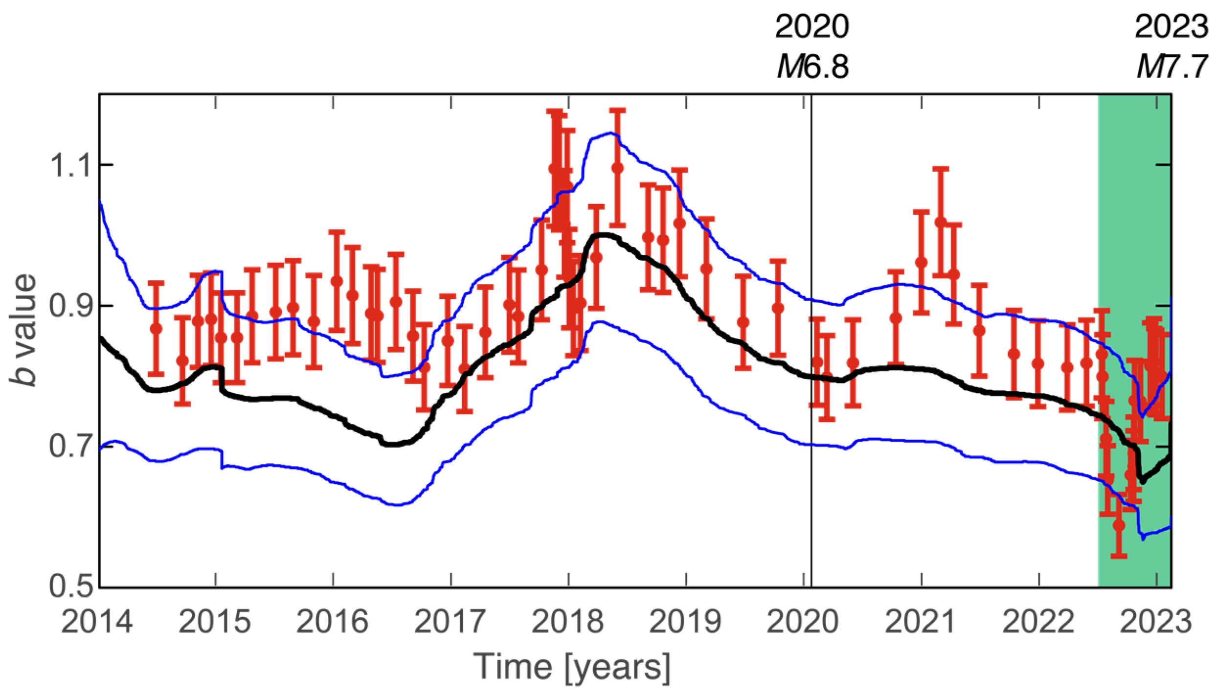
Kwiatek et al. [10] showed seismicity transients: low b values and seismic activation starting approximately 8 months before the 2023 M7.7 quake in the region within a 50 km radius surrounding the future M7.7 epicenter. We used the same region to confirm the former transient based on a b-value method different from that of Kwiatek et al. [10]. In our method [24], the b-value function of time is represented by a broken line connecting the sequence of quakes under a smoothness constraint in piecewise slopes using the empirical Bayesian smoothing technique. Unlike Kwiatek et al. [10], the method we used does not assume a moving window. Therefore, it has the advantage of obtaining unbiased b values as a function of time [24]. Regardless of whether the previous method [10] or our method was used, the results were similar (Figure 2), enhancing the robustness of our conclusion. The lowest b values (~0.6) during the period from July 2022 to immediately before the M7.7 quake are related to two clusters, referred to as C1 and C2 by Kwiatek et al. [10].

Figure 2.
Timeseries of b values in the circle with a 50 km radius centered at the M7.7 epicenter for the period from 2014 to immediately before the M7.7 quake. The circular region and the time period are the same as those used by Kwiatek et al. [10]. The b values (black) with error bars showing 95% confidence intervals (blue) are shown and are based on the AFAD catalog. Also included for comparison is the time dependence of b (red) shown in Kwiatek et al. [10]. These authors used a moving event window of 120 events and plotted each calculated b value at the time of the last event in each window, where the b values were computed by using the b-positive method [43]. The green region shows the period from 1 July 2022 to immediately before the M7.7 quake. The vertical line indicates the moment of the 2020 M6.8 quake.
One possible avenue to further strengthen our analysis is to consider different b-value estimation methods, such as the b-positive method [43], the b-more-positive method [44], and the b-value method using particle filtering and the state space model [45]. Our future analysis requires consideration of these methods, although the b-positive approach was taken by Kwiatek et al. [10].
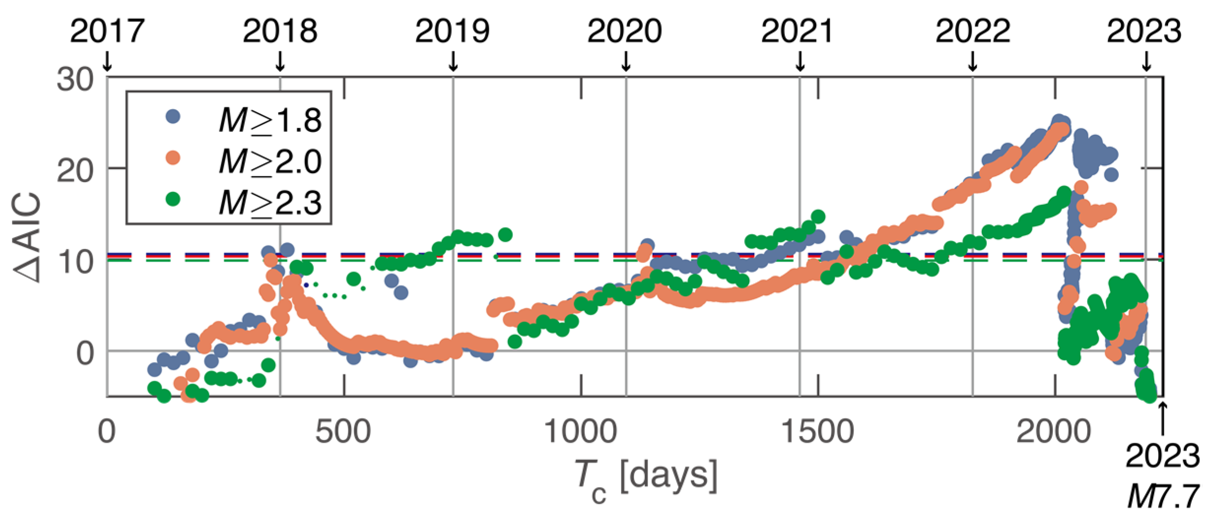
We next showed that the latter transient (seismic activation) is statistically significant by conducting a change point analysis. For this analysis, ΔAIC = AICsingle − AIC2stage was used as a function of the change point time Tc [20,24,46,47]. Here, AICsingle is the AIC for the standard (single) ETAS model that considers a constant θ value over time, and AIC2stage is the AIC for the two-stage ETAS model that considers different θ values in subperiods before and after Tc, where both models are fitted to quakes of M ≥ Mth. If ΔAIC ≥ 2q, fitting of the two-stage model to the data is better than that of the single model and it detects candidate changes in occurrence rate, where q is the degree of freedom to search for the best candidate Tc from the data. q depends on the sample size (number of quakes of M ≥ Mth) [48,49]. The result for Mth = 2 (red data in Figure 3) shows that the two-stage ETAS model was much better than the single ETAS model during Tc = 1600~2100 days, where we used the same events in the region as those used by Kwiatek et al. [10] during the period from 1 January 2017 to immediately before the M7.7 quake in the AFAD catalog. The most significant Tc was 2015 days (9 July 2022). The results for Mth = 1.8 (blue data) and 2.3 (green data) indicate that the most significant Tc values were 2008 days (2 July 2022) and 2019 days (13 July 2022), respectively. This feature, i.e., that the most significant Tc values are about 8 months before the M7.7 quake, was observed regardless of Mth values.

Figure 3.
ΔAIC as a function of Tc for the period from 1 January 2017 to immediately before the 2023 M7.7 quake. Blue, red, and green data are based on quakes of M ≥ 1.8, 2.0, and 2.3, respectively, within a 50 km radius from the M7.7 epicenter. In case that the model-fitting analysis did not converge, ΔAIC at the corresponding Tc is shown by a small dot. Vertical lines indicate 1 January for 2018, 2019, …, 2023. Horizontal dashed lines represent 2q for M ≥ 1.8 (blue), 2.0 (red), and 2.3 (green) overlap.
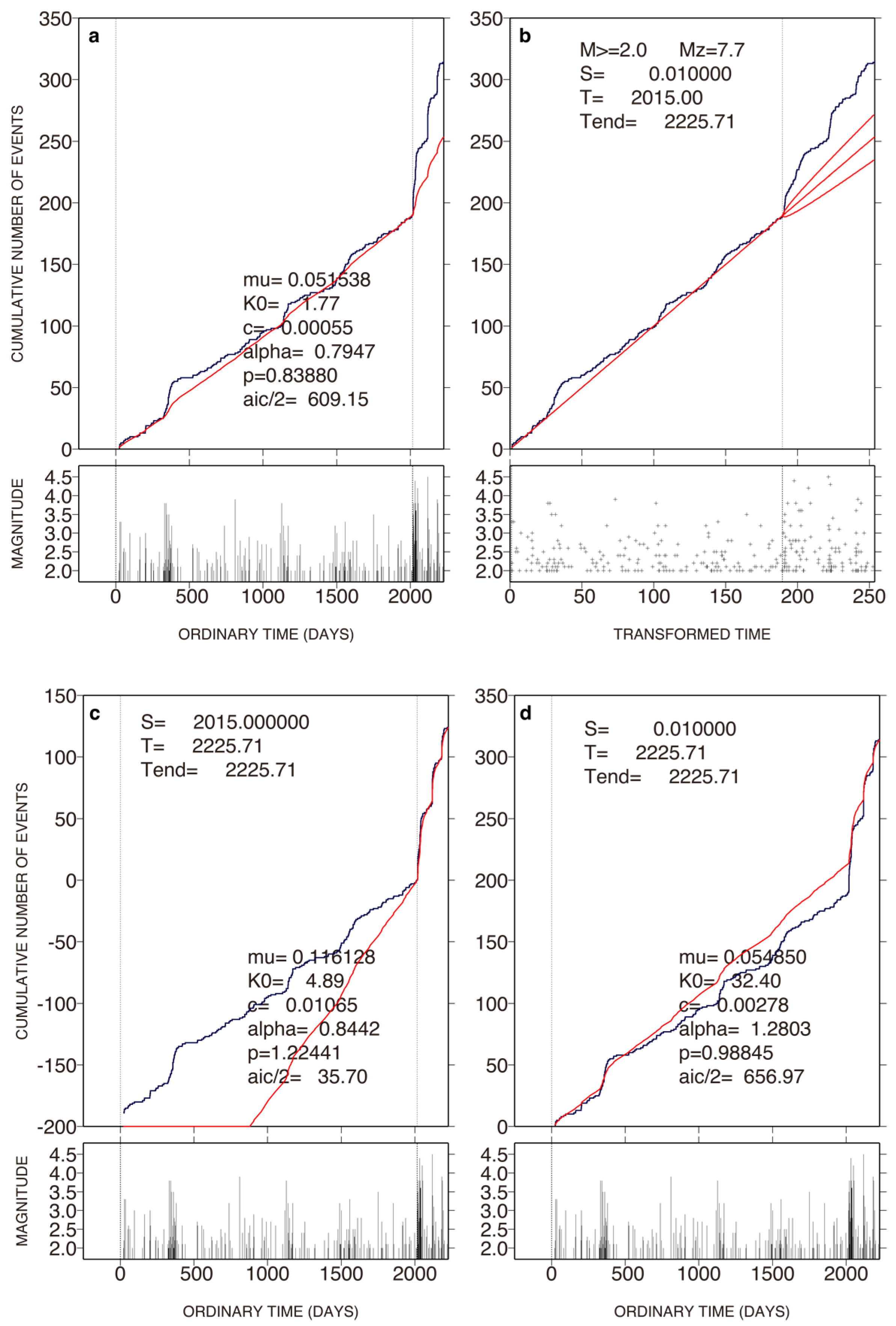
We fitted the ETAS model to quakes (M ≥ 2) before Tc = 2015 days (9 July 2022) (Figure 4a,b). For this fitting, three time intervals were assumed [24]. One interval is the target interval, for which θ was computed. The seismicity in this interval may be affected by quakes which occurred before this interval due to the long-lived nature represented by the OU relation. To take this effect into account, another time interval, which is precursory to the target interval, was chosen. This interval is called the precursory interval, and quakes in this period are included in the computation. The precursory and target intervals are defined by 0 to S and S to T, respectively. The third time interval defined by T to Tend is called the prediction interval. θ in this interval is the same as that computed for the target interval. We set S = 0.01 days, T = Tc = 2015 days (9 July 2022), and Tend = 2225.71 days (immediately before the M7.7 quake). The occurrence rate (black) after T = Tc = 2015 days (during the prediction interval) was larger than the extrapolated rate (red), indicating relative activation (Figure 4a,b). Here, the extrapolated rate is the occurrence rate computed by using the ETAS model, in which θ was obtained by fitting to quakes (M ≥ 2) before T = Tc = 2015 days (the target interval). We confirmed the relative activation by switching the prediction and target intervals (Figure 4c). We also confirmed the poor fitting of the standard (single) ETAS model to quakes during the entire period (Figure 4d).
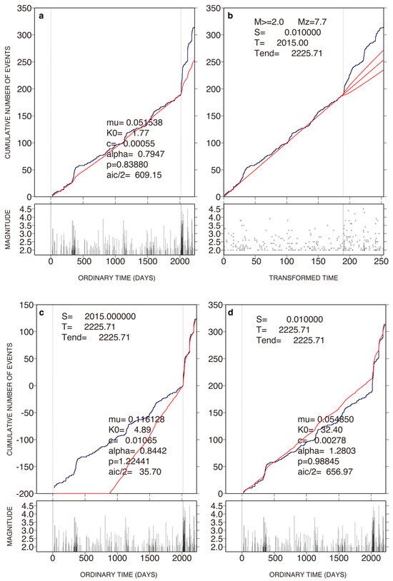
Figure 4.
Change point analysis. Plot of cumulative function of M ≥ 2.0 quakes against ordinary time in (a) and transformed time in (b) is given, showing the ETAS fitting in the target interval is from 2017 to 9 July 2022 (the most significant Tc = 2015 days for M ≥ 2.0 shown in Figure 3), and then extrapolated until immediately before the 2023 M7.7 quake. The parabola represents the 95% confidence intervals of the extrapolation [20,24,46]. Because K0 differs depending on reference magnitude Mz [20], we used Mz = 7.7. This value (Mz = 7.7) is the largest magnitude in this study. Below each larger panel, an M–time diagram in the small panel is given. (c) Same as (a) except that the target is the later time interval after 9 July 2022. (d) Same as (a) except that the target is the entire time interval.
5.1.2. Background Activity and Clustering Activity
We further analyzed seismicity during the 8 months before the 2023 M7.7 quake to explore the reason for the change in the rate of quake occurrences (Figure 5). We took a reductionism approach by decomposing all quakes into Poisson background activity and clustering activity. We measured μ (a solo parameter of the Poisson background activity) and K0 (a parameter representing the clustering activity) while the other three parameters (α, c, p) were constants. We used a non-stationary ETAS approach [24,46,49,50] to seismicity before the M7.7 quake. The standard (single) ETAS model, which is the stationary ETAS model, can be extended to the non-stationary ETAS model in such a way that μ and K0 are time-dependent functions. The function μ(t) is represented by a broken line connecting the sequence (ti, μ(ti)) for the i-th quake using a Bayesian function. Similarly, K0(t) is represented by a broken line connecting the sequence (ti, K0(ti)).
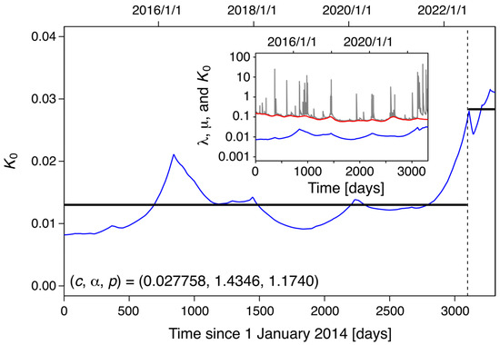
Figure 5.
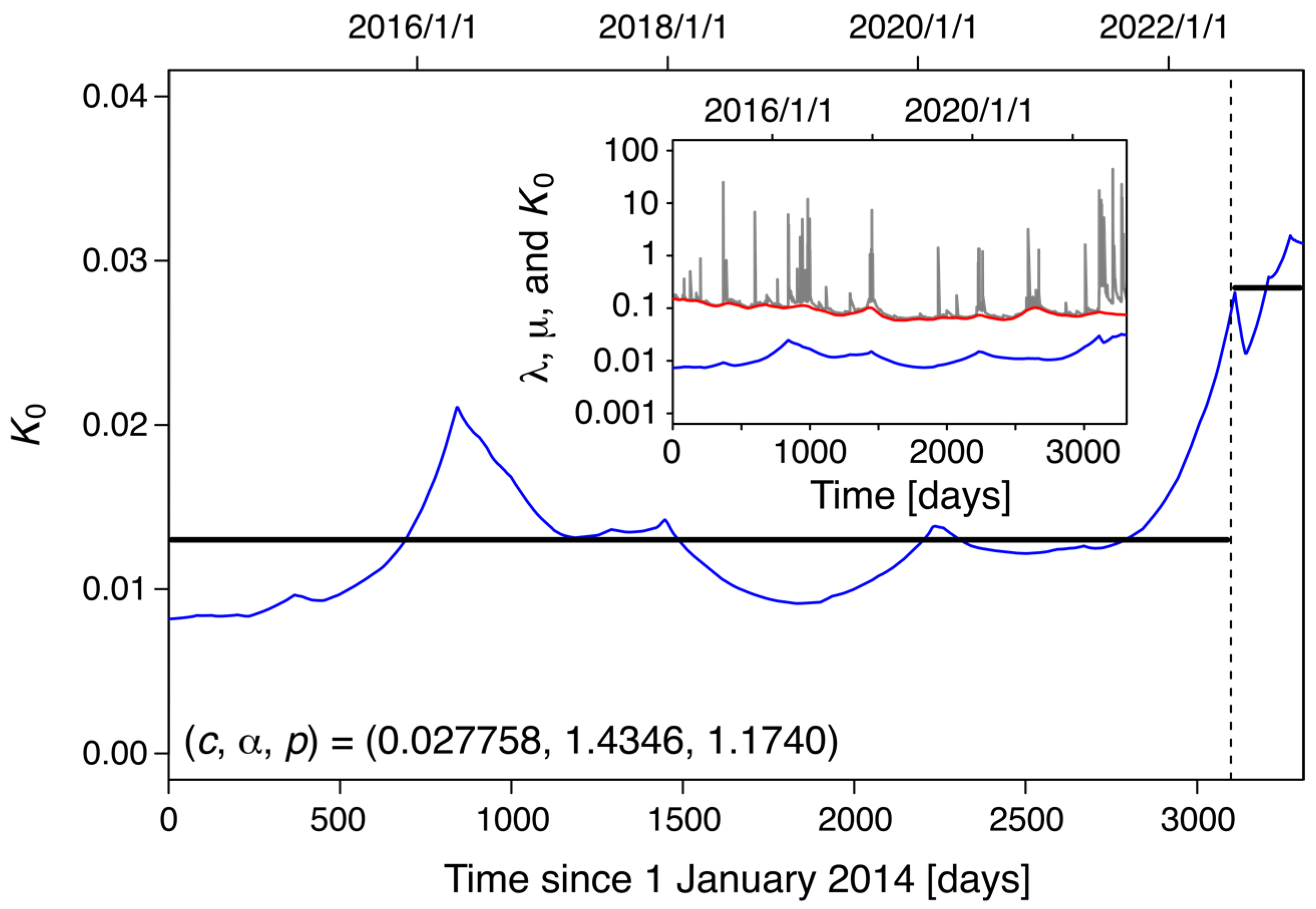
K0 as a function of time. Quakes with M ≥ 2 (Mth = 2) for the period from 2014 to immediately before the M7.7 quake within a 50 km radius around its epicenter were used. Vertical dashed line indicates 9 July 2022 (Tc = 2015 days in Figure 3). Horizontal lines indicate the mean values of K0 for the periods before and after Tc = 2015 days. Inset shows λ (grey), μ (red), and K0 (blue) as a function of time, while c, α, and p are constants. For M ≥ 1.5, see Figure S1.
We obtained the α, c, and p values for the standard (single) ETAS fitting to the quakes (M ≥ 2) over the period from 2014 to immediately before the M7.7 quake in the region within a 50 km radius surrounding the future M7.7 epicenter. Then, the obtained α, c, and p values were assumed to be applicable to the non-stationary ETAS model with μ(t), K0(t), and λ(t). Namely, the α, c, and p values were independent of t. Given the predefined α = 1.43, c = 0.028, and p = 1.17 for Mth = 2 (M ≥ 2), μ (red), K0 (blue), and λ (grey) were computed for each quake (inset of Figure 5). Visual inspection shows that μ was nearly constant over time. However, K0 was visually larger after mid-2022 than before it, although the timeseries of K0 before mid-2022 showed one tall peak in 2016. Focusing on the time-dependent K0, in Figure 5 we included the average (horizontal solid line) of the K0 values for the periods before and after 9 July 2022 (Tc = 2015 days) (vertical dashed line). The average of the K0 values after 9 July 2022 was nearly equal to K0 values around the tall peak in 2016. The result shows that K0 was larger after the start of seismic activation than before it, suggesting that clustering had an influence on the months-long activation surrounding the M7.7 quake nucleation region. The increase in K0 is consistent with the emergence of clusters C1 and C2 [10] within 8 months prior to the M7.7 quake. The same analysis was conducted for M ≥ 1.5 (Figure S1), supporting our result.
5.1.3. Slip Distribution of the M7.7 Quake and Preceding Seismicity
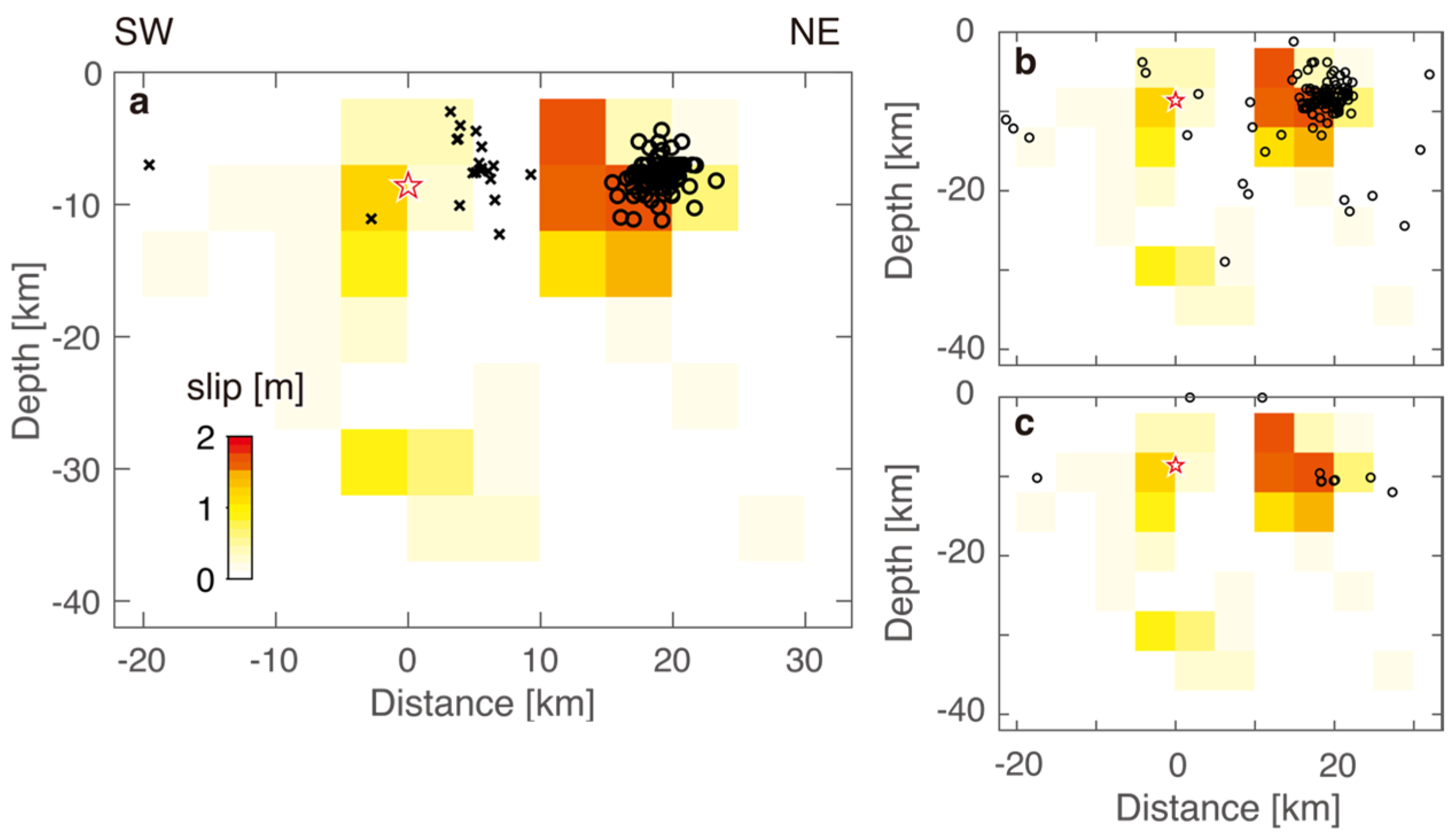
A cross-sectional view (Figure 6a) shows the slip distribution on segment 2 where the M7.7 quake initiated [2] and seismicity after the start of the activation (circles) (from 1 July 2022 to immediately before the M7.7 quake). To create this cross-section, we used the AFAD catalog and retrieved M ≥ 2 events within 7.5 km from the segment (width of 15 km). The retrieved events mostly consisted of events within cluster C2 [10]. An area of high-slip values of >1.5 m (red) was separated by about 10 km from the M7.7 hypocenter (star). This high-slip area overlaps with seismicity after the start of the activation (circles). A similar result was obtained (Figure 6b) using the catalog of Kwiatek et al. [10], in which events during the period from 1 January 2023 to immediately before the M7.7 quake were included. We considered M ≥ 0.5 events because the Mc for the catalog was 0.5 [10]. We similarly investigated the catalog of Lomax [16]. The number of quakes (M ≥ 1.5, from 1 January 2023 to immediately before the M7.7 quake) was inadequate (Figure 6c), although the result is consistent with those in Figure 6a,b. Given that cluster C2 contributed to the display of low b values (b = 0.6 [10]), our result indicates that the zone of low b values coincided with the location of a future high-slip area on segment 2. This is similar to the result obtained by Nanjo et al. [30], who compared the slip distribution of the 2011 M9 Tohoku quake in Japan and the distribution of areas with low b values of seismicity from 2008 to immediately before the Tohoku quake. Those authors showed that the zones of extremely low b values coincided remarkably with locations of an extremely large co-seismic slip.
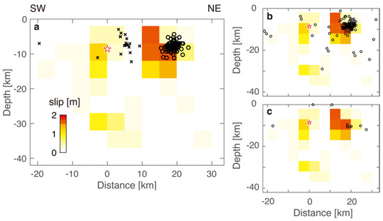
Figure 6.
Slip distribution along segment 2, from which the M7.7 quake initiated [2]. Star indicates the M7.7 hypocenter. (a) We used the AFAD catalog. Events (M ≥ 2) within 7.5 km from this segment (width of 15 km) are shown by circles and crosses. Circles indicate events from 1 July 2022 to immediately before the M7.7 quake. Crosses indicate the same as circles for events during 23 October 2017 to 21 January 2018 (2017.9–2018.1 decimal years). (b) Same as (a), but we used the catalog of Kwiatek et al. [10]. Circles indicate events (M ≥ 0.5) within 7.5 km from the segment from 1 January 2023 to immediately before the M7.7 quake, where Mc = 0.5 is the completeness magnitude according to Kwiatek et al. [10]. (c) Same as (b), but we used the catalog of Lomax [16]. Circles indicate events (M ≥ 1.5) within 7.5 km from the segment from 1 January 2023 to immediately before the M7.7 quake, where M = 1.5 is the minimum magnitude for quakes recorded in the catalog of Lomax [16].
Also included in Figure 6a is the distribution of a swarm (crosses) in late 2017 to early 2018, shown as an upward convex around 340 days in ordinary time in Figure 4a or 40 in transformed time in Figure 4b. This swarm corresponds to cluster C7 [10]. The majority of this swarm overlaps with a low-slip area (white to light yellow). Cluster C7 displayed a high b value (b = 0.9 [10]). The observation between a high b value and a low slip is also consistent with a previous study [30].
5.2. Post-Doublet-Quake Sequence
5.2.1. Seismicity Immediately After the Doublet Quakes
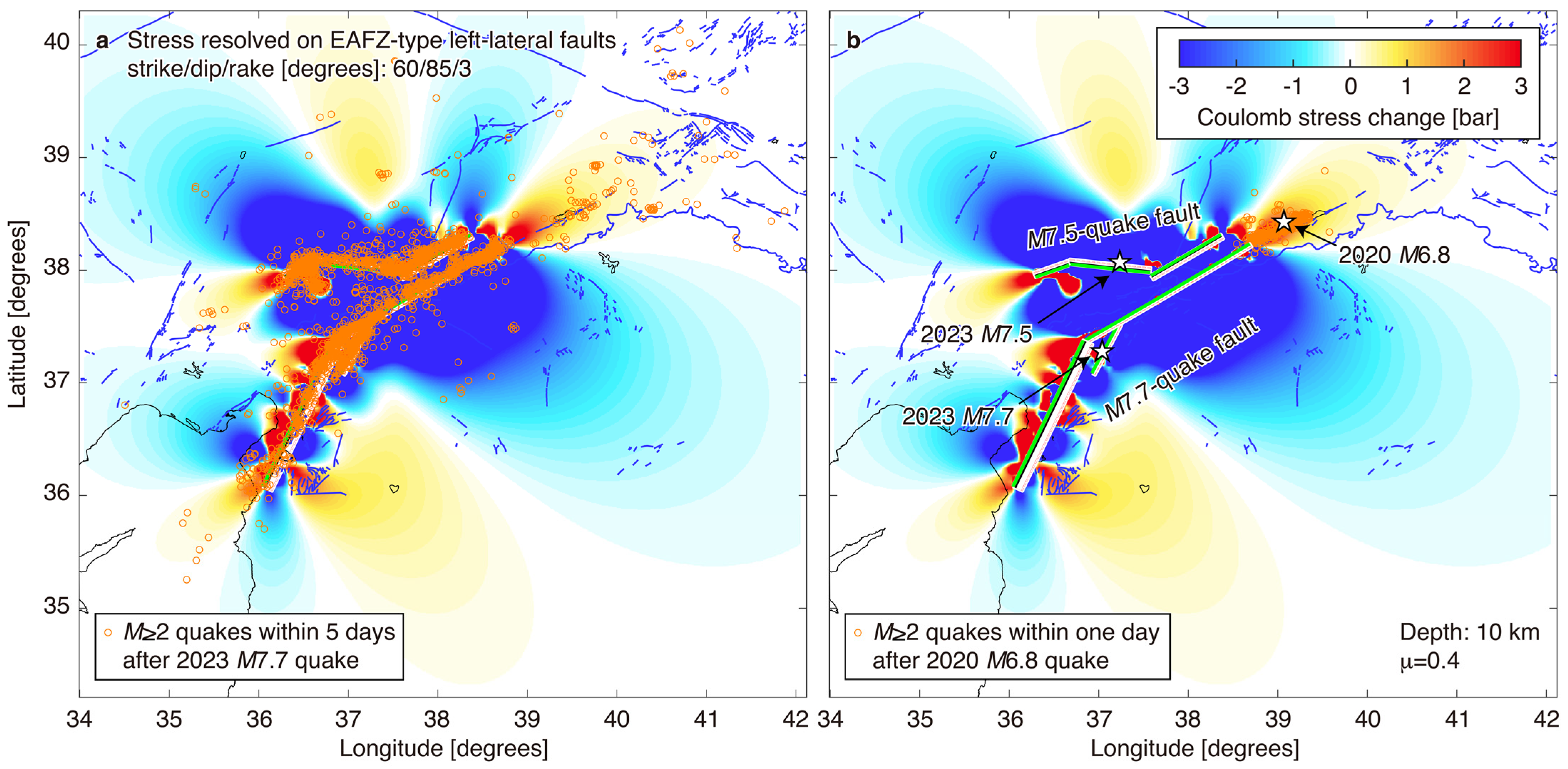
We calculated Coulomb stresses imparted by the doublet quakes and their relationship to seismicity within 5 days after the M7.7 quake (Figure 7a) using the USGS source models of the M7.7 and 7.5 quakes [2,3] and the AFAD quake catalog. In creating Figure 7a, the stresses were resolved on idealized faults oriented parallel to segment 1 (strike/dip/rake = 60°/85°/3°) [2] and, therefore, were similar to the broad character of the EAFZ. We observed a lack of seismic activity at the zone of increase in Coulomb stress beyond the north end of the M7.7 rupture, noting that the area, which lacked seismic activity, coincided with the area of the M6.8 rupture (Figure 7b). To create this figure, the same Coulomb stress calculation as was used in Figure 7a was conducted, but we used seismicity within 1 day after the 2020 M6.8 quake, which outlined the 2020 M6.8-quake source. Stress in the area beyond the north end of the M7.7 rupture was released by the 2020 M6.8 quake so that the increase in stress imparted by the doublet quakes was insufficient to induce the following events in this area. This is consistent with the result obtained by Toda and Stein [5], who showed that the 2020 M6.8 quake locally dropped the stress by ~10 bars, and the M7.7 quake then increased the stress there by 1–2 bars, resulting in a hole in seismicity after the M7.7 quake.
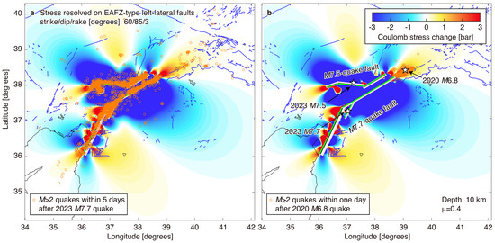
Figure 7.
Coulomb stress changes as a result of the 2023 M7.7 and 7.5 quakes. (a) Changes in stress imparted to surrounding faults under the assumption that all faults are parallel to the main rupture (segment 1) of the M7.7 quakes. Circles indicate events (M ≥ 2 and depths shallower than 40 km) within 5 days after the M7.7 quake occurred. Green lines indicate the M7.7- and 7.5-quake fault models [2,3]. Blue lines indicate active faults. (b) Same as a for events within 1 day after the occurrence of the 2020 M6.8 quake. Stars indicate the epicenters of the M6.8, 7.7, and 7.5 quakes.
5.2.2. Seismicity Until the M6.4 Quake
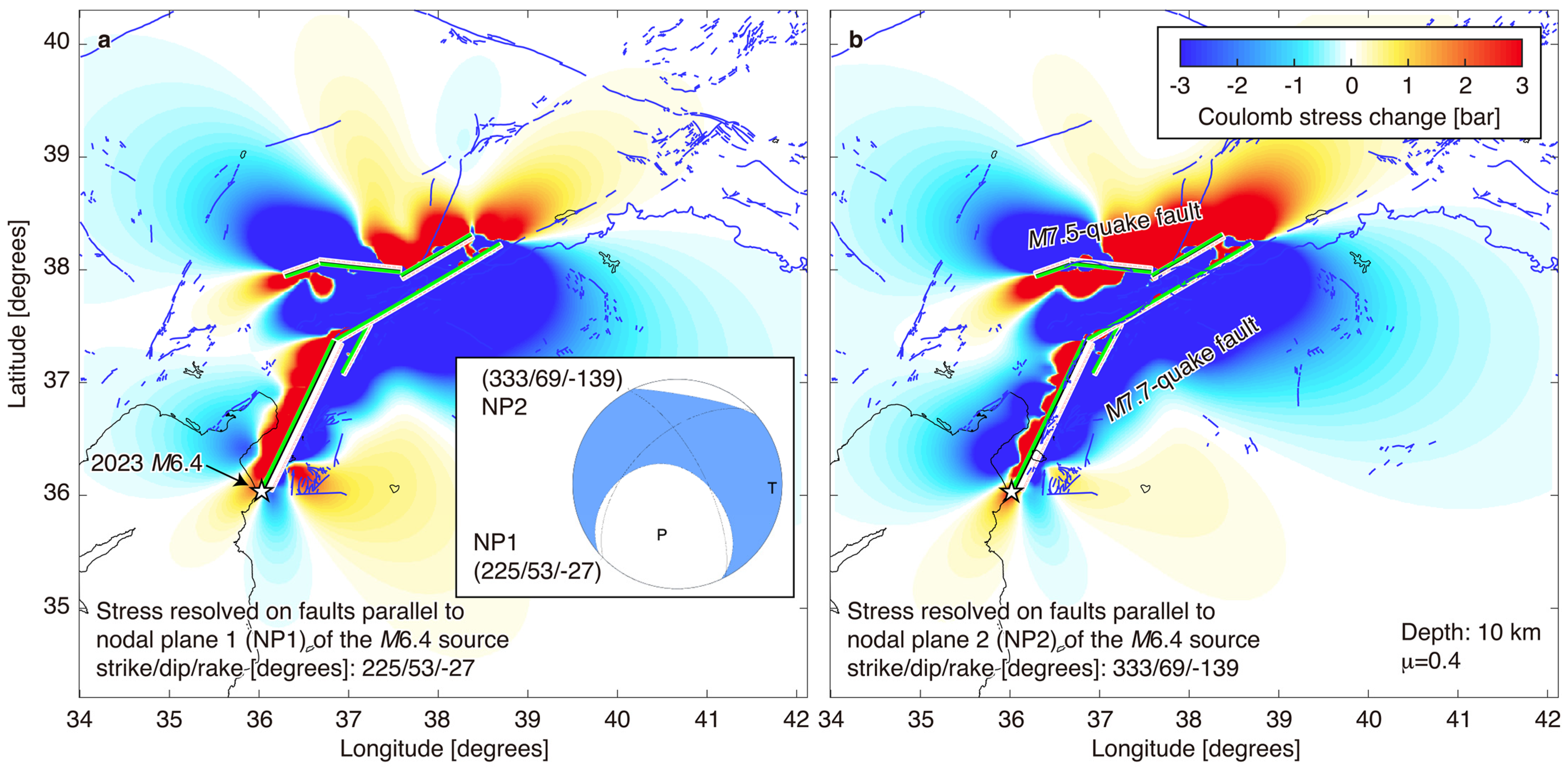
The largest event (M6.4) after the doublet quakes occurred on 20 February 2023 in an area around the south end of the M7.7 rupture. In creating Figure 8a, we conducted the same stress calculation as that for Figure 7a, but resolved stresses on faults oriented parallel to NP1 with strike/dip/rake = 225°/53°/−27° of the M6.4 source [13]. The fault that ruptured during the M6.4 quake was promoted toward failure. The same resolution was conducted for NP2 with strike/dip/rake = 333°/69°/−139°, and a similar result was obtained (Figure 8b). Över et al. [11] obtained a result consistent with Figure 8a.
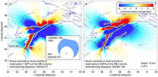
Figure 8.
Same as Figure 7 for stresses resolved on faults parallel to NP1 of the 20 February 2023 M6.4 source [13] in (a) and NP2 in (b). Star indicates the epicenter of the M6.4 quake. Inset shows beach ball indicating the focal mechanism of the M6.4 quake [13]. NP1 and NP2 are shown. The P and T axes are also plotted.
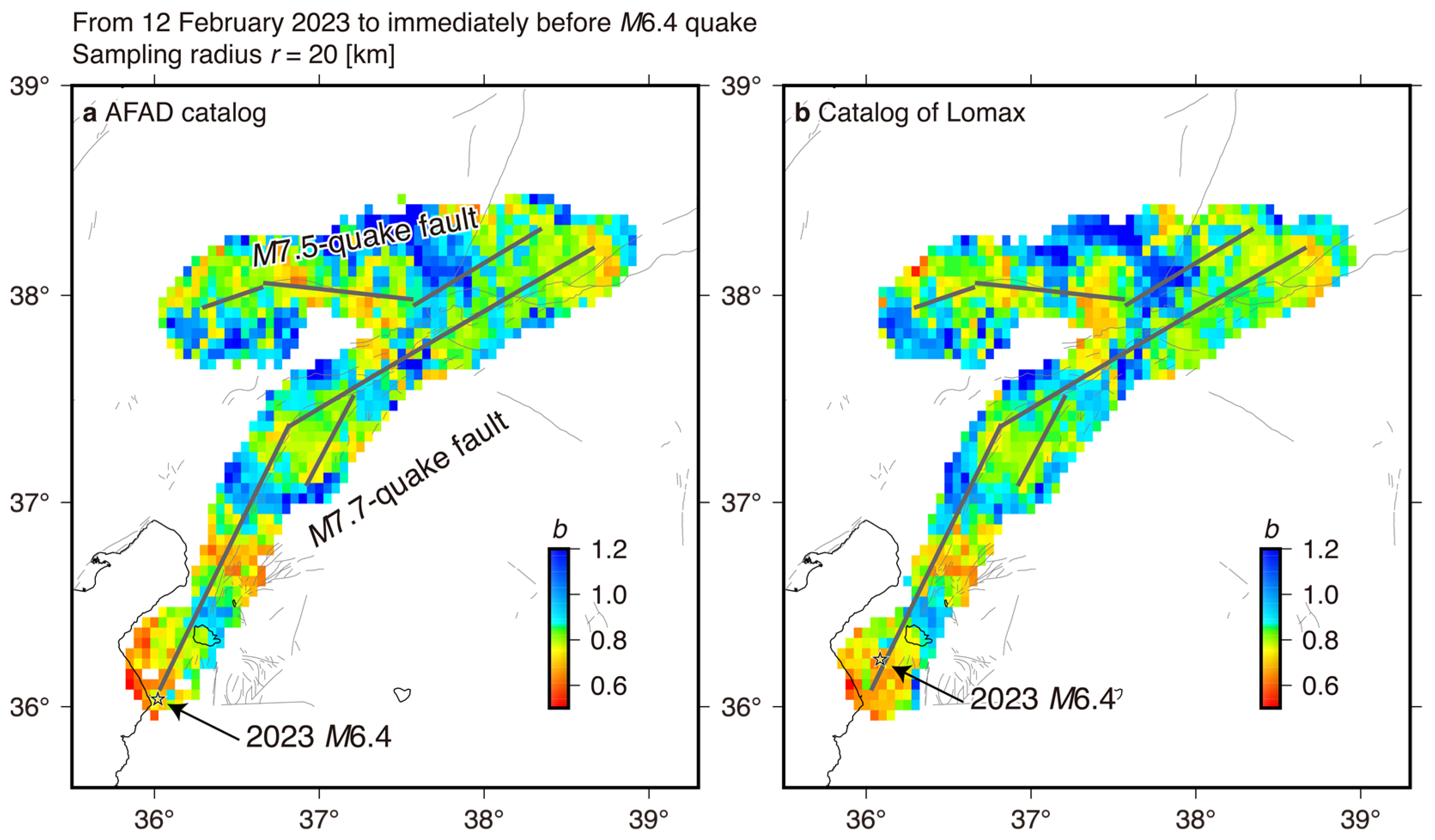
A map view based on data from the AFAD catalog for the period from 12 February 2023 to immediately before the M6.4 quake (Figure 9a) shows that the eventual epicenter fell in a region of low b values (red), where the period until 11 February 2023 was not considered to remove the influence of the main aftershock activity, revealing strong time-dependent variability in b. To create this map, we computed b values [21,22] for events falling in a cylindrical volume with height = 30 km and sampling radius r = 20 km, centered at each node on a 0.05° × 0.05° grid, and plotted a b value at the corresponding node. According to a previous study [51], we mapped b values for different r values, where r = 10, 15, …, 30 km, to find the optimal r value (Figures S2 and S3). A nearly identical pattern of b values was observed when sampled with r = 15–20 km. Using r = 10 km did not reveal details because it only reduced coverage. Sampling with r ≥ 25 km resulted in smoothed b values. For r = 30 km, the low b-value zone lost its crispness and moved toward the outside. This is because the small volumes containing information about the low b values were located at the edge of seismically active regions. At the locus of the b-value anomaly, the sample became a mixture of different distributions when r was increased. As a result, the anomaly was visually reduced. Thus, the optimal r was in the range of 15–20 km (Figure S2). In Figure 9, r = 20 km was used, but using r = 15 km, which slightly reduced coverage, did not change the conclusion. The corresponding Mc maps are given in Figure S2, where Mc was simultaneously calculated when calculating the corresponding b value [22]. A similar feature was observed in Figure 9b by using the catalog of Lomax [16], where the procedure to map b values was the same as that used for Figure 9a (see Figures S4 and S5).
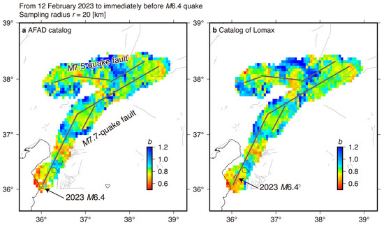
Figure 9.
Map views of b values before the 20 February 2023 M6.4 quake (star), using the AFAD catalog in (a) and the catalog of Lomax [16] in (b). In (a,b), quakes during the period from 12 February to immediately before the M6.4 quake were used. The M6.4-quake epicenter (star) in (a) is different from that in (b) because the epicenter of the M6.4 quake in the AFAD catalog is different from that in the catalog of Lomax [16]. Thick grey segments show fault models of the M7.7 and 7.5 quakes [2,3]. Thin grey lines indicate active faults.
5.2.3. Seismicity Until the M5.9 Quake
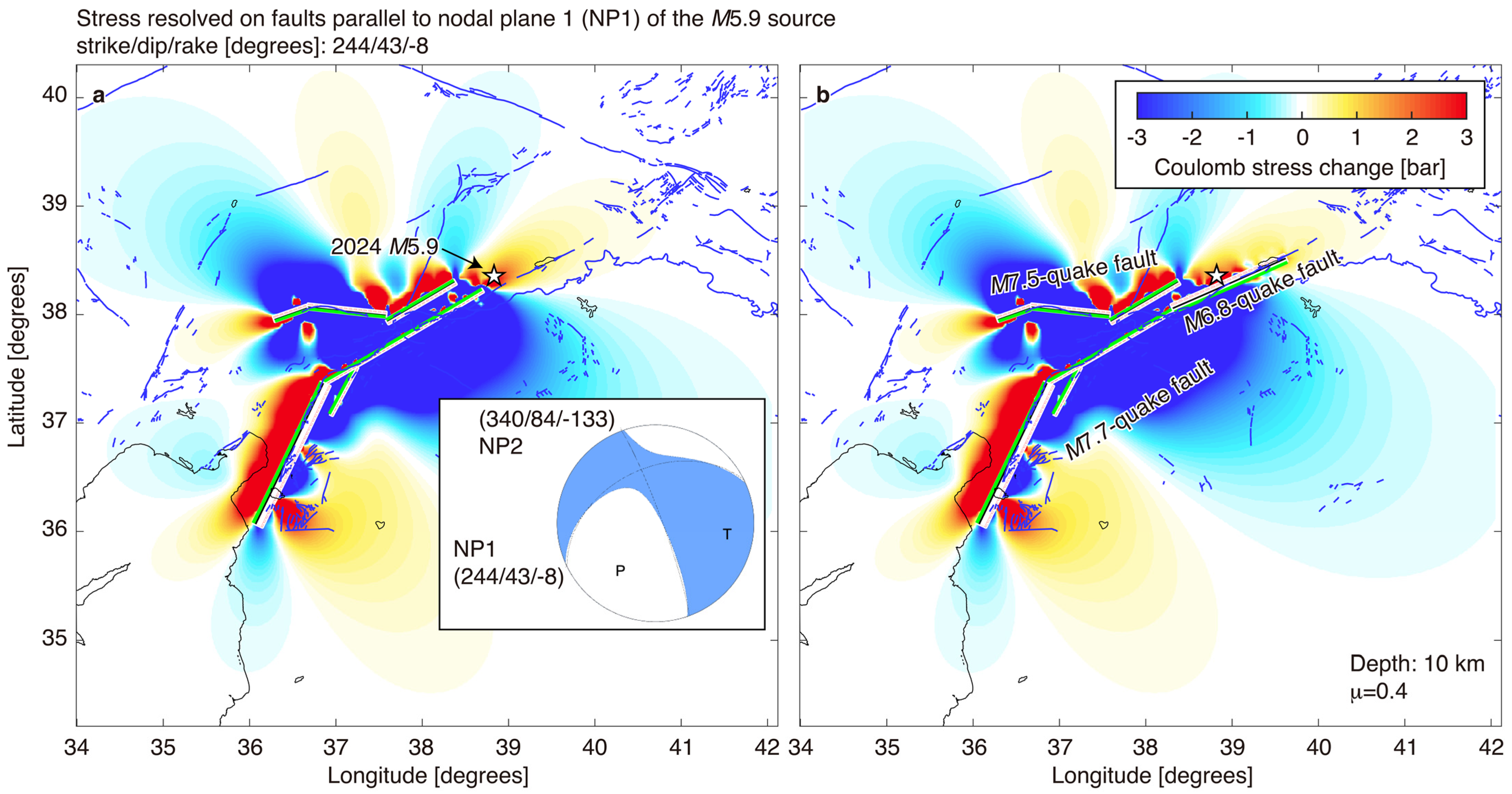
The second-largest event (M5.9) after the doublet quakes occurred on 16 October 2024 in an area around the north end of the M7.7 rupture. The same stress calculation as in Figure 7 was conducted, but different receiver faults [14] were used. Namely, we used two NPs of the M5.9 source: strike/dip/rake = 244°/43°/−8° in Figure 10a and 340°/84°/−133° in Figure S6b. The result shows that the fault that ruptured during the M5.9 quake was promoted toward failure by the double quakes, irrespective of the plane that was used (Figure 10a and Figure S6b). We conducted the same stress calculation as in Figure 10a and Figure S6b, except that the 2020 M6.8-quake fault was added into source faults, where the finite fault model of this quake is based on the work by the USGS [4]. A similar feature was observed (Figure 10b and Figure S6a).
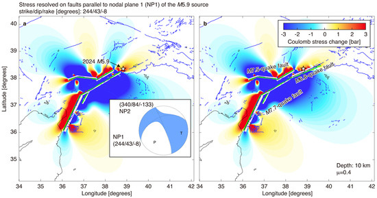
Figure 10.
Coulomb stress changes resolved on faults parallel to NP1 of the 16 October 2024 M5.9 source [14]. (a) Changes in stress imparted by the M7.7 and 7.5 quakes in 2023. Star indicates the epicenter of the M5.9 quake. Inset shows beach ball indicating the focal mechanism of the M5.9 quake [14]. (b) Changes in stress imparted by the M6.8 quake in 2020 and the M7.7 and 7.5 quakes in 2023. For NP2, see Figure S6.
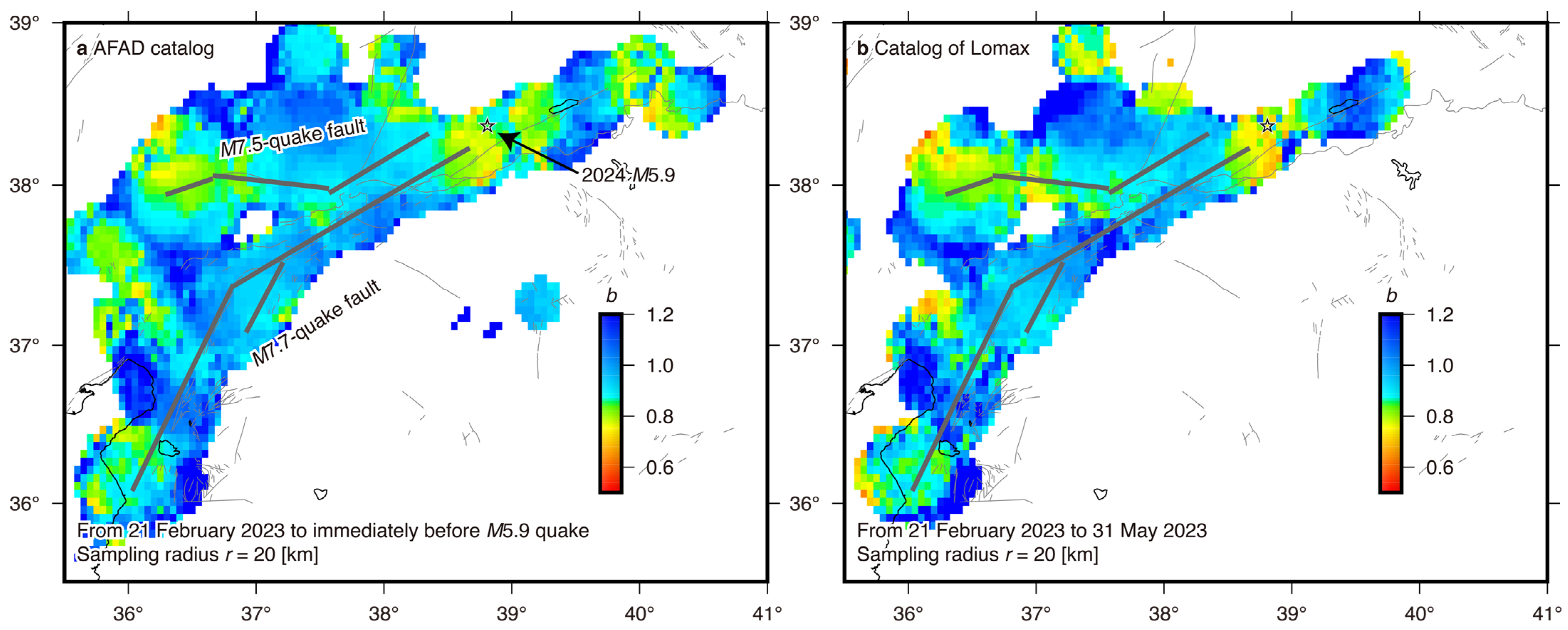
A map view based on use of the AFAD catalog for the period from 21 February 2023 to 15 October 2024 shows a zone of relatively low b values (yellow to green) around the future epicenter (Figure 11a). The mapping procedure was the same as that in Figure 9a. The optimal r was in the range of 15–20 km (Figures S7 and S8). Similar to Figure 9a, we decided to use r = 20 km in Figure 11a. This feature generally appears when using the catalog of Lomax [16] (Figure 11b, Figures S9 and S10).

Figure 11.
Map views of b values before the 16 October 2024 M5.9 quake (star), using the AFAD catalog in (a) and the catalog of Lomax [16] in (b). Grey segments show fault models of the M7.7 and 7.5 quakes [2,3].
6. Discussion
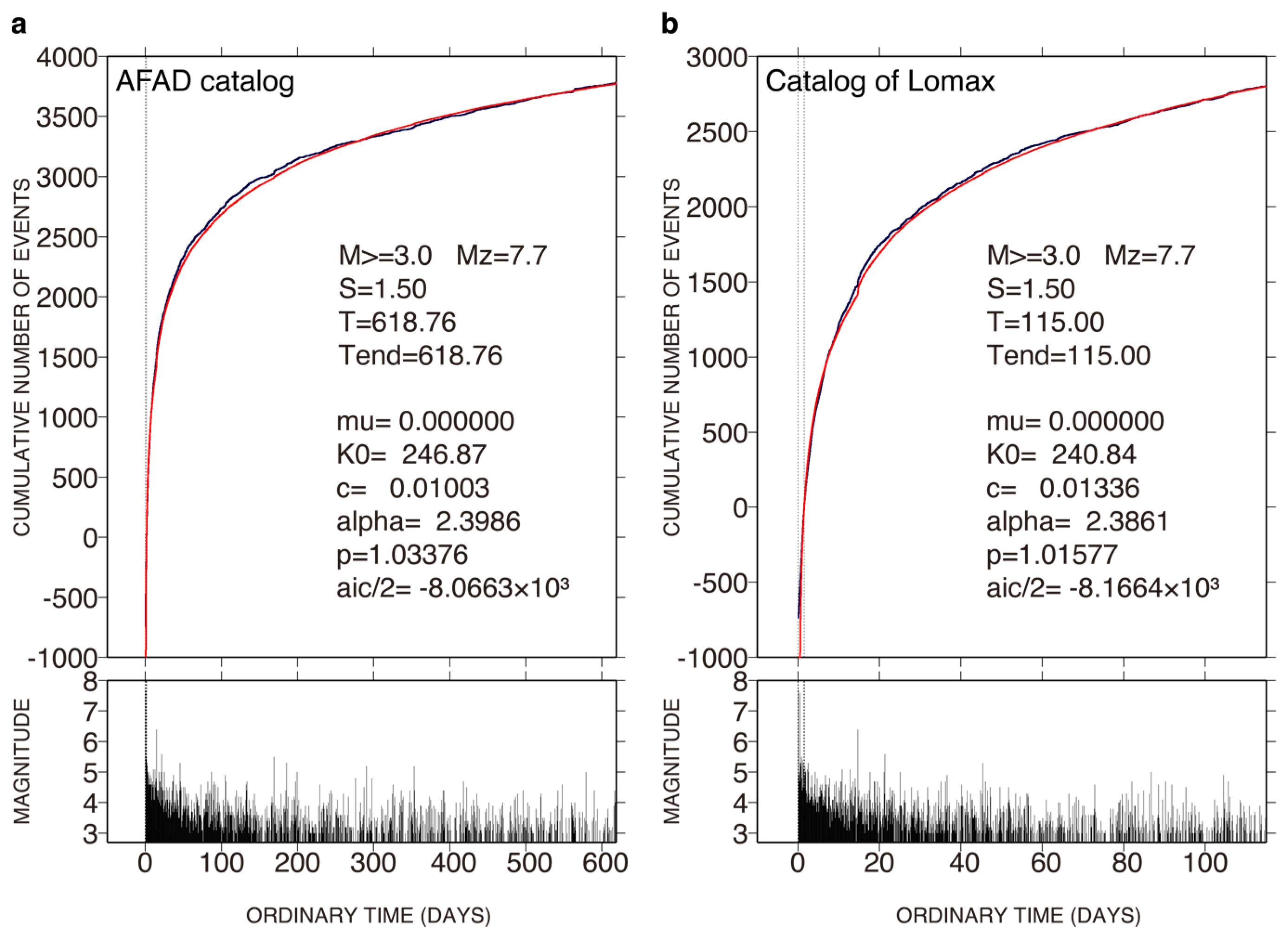
As was pointed out in Section 2, we discuss the need for a comparison of the duration of the post-doublet-quake sequence between our study and a previous study [5] to provide information that might possibly be used when evaluating a time-dependent seismic hazard along the NAFZ. As the basis of this comparison, we first confirmed that the overall seismicity after the doublet quakes around the causative faults decayed with time (black curve in Figure 12a), where M ≥ 3 quakes in the AFAD catalog during the period from the M7.7 quake to 16 October 2024 in the study region shown in Figure 11 were used (see also Figure S11). Visual inspection (Figure 12a) shows that the standard (single) ETAS model (red curve) fits the data after the M7.7 quake well, suggesting no pronounced activation and quiescence. Similar results were obtained for M ≥ 4 (Figure S11). The results were not induced by catalog selection bias because similar results were observed when using the catalog of Lomax [16] (Figure 12b and Figure S12). The well-fitted results of the standard (single) ETAS model to the data (Figure 12 and Figures S11 and S12) allowed us to assume that use of the OU relation is sufficient to capture an essential aspect of seismicity decay following the doublet quakes and to estimate the expected duration of the post-doublet-quake sequence, as described below.
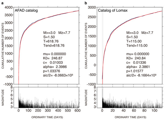
Figure 12.
ETAS fitting to quakes after the M7.7 quake. (a) Cumulative function of M ≥ 3.0 quakes in the AFAD catalog is plotted against ordinary time, showing the ETAS fitting in the target interval from 1.5 days after the M7.7 quake to 16 October 2024, where the precursor interval is from the moment of the M7.7 quake to 1.5 days after the M7.7 quake. (b) Same as (a), but using the catalog of Lomax [16].
As was performed by Toda and Stein [5], we correlated the quake sequence with the OU relation, where we used events of M ≥ 3 (green circles in Figure 13) in the AFAD catalog (from immediately after the M7.7 quake to 16 October 2024 in the region considered for Figure 11). A similar correlation was obtained by using the catalog of Lomax [16] (green crosses). We used the ordinary occurrence rate of 0.3 M ≥ 3 quakes per day (horizontal green line) based on the number of M ≥ 3 quakes in the AFAD catalog during the period from 2014 to immediately before the 2020 M6.8 quake in the region considered for Figure 11. The intersection between the horizontal green line and the green curve shows an expected duration of about 1–2 × 10³ days. Similar expected durations were obtained for M ≥ 2 (red) and M ≥ 4 (blue) (Figure 13).
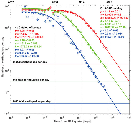
Figure 13.
Number of quakes per day, λOU, as a function of time t since the M7.7 quake is correlated with the OU relation. Quakes of M ≥ 2 (red), M ≥ 3 (green), and M ≥ 4 (blue) in the AFAD catalog (circles and solid curves) were used. The parameter values of the OU relation are given at the upper right corner. The standard deviations of the respective parameters of the bootstrap samples were used to define the corresponding error bars. Vertical lines indicate the moments of the M7.5, 6.4, and 5.9 quakes. Horizontal line indicates the rate of quakes of M ≥ 2 (red), M ≥ 3 (green), and M ≥ 4 (blue) obtained for the period from 2014 to immediately before the 2020 M6.8 quake. Also included for comparison is the correlation with the OU relation when using the catalog of Lomax [16] (crosses and dashed curves).
Our expected duration was longer than that (1–2.5 years) obtained by Toda and Stein [5]. We assumed a more stable fitting of the OU relation to the data in the present study than in the previous study. This is because Toda and Stein fitted the OU relation to quakes during the period of about 100 days since the M7.7 quake, whereas we completed this process for a period of 618 days since the M7.7 quake, i.e., the period (about 100 days) considered by Toda and Stein was shorter than the period (618 days) we considered. Similar to Toda and Stein [5], we considered the quake sequence of M ≥ 4.5 to obtain the estimated duration (Figure S13). This sequence is correlated with the OU relation. An ordinary occurrence rate of 0.006 M ≥ 4.5 quakes per day was used. The expected duration was about 1–2 × 10³ days. This is similar to the expected durations obtained for M ≥ 2, 3, and 4, and longer in a previous study [5].
During the 20th century, much of the northern section of the EAFZ ruptured, as described in Section 2. Starting with the 2020 M6.8-quake sequence, much of the southern section ruptured (Figure 1). Regional and global quake magnitude frequency distributions obey a GR relation (e.g., [29,30,31,51,52]), but it is unclear if individual fault zones do. Namely, the frequency of quake size on fault zones is distributed in a GR relation or characteristic. Parsons et al. [53] used data from California, USA, and found that individual fault zones have characteristic magnitude distributions, with a greater number of large quakes relative to small quakes than expected from a GR trend (e.g., [54]). There is no doubt that the M7.7 quake was not the almighty quake [55], which would rupture an entire plate boundary at once and leave no stress that could produce any other kind of quake. To rephrase it, the almighty quake is the extreme end of characteristic earthquake behavior. The GR relation is the other end member of the spectrum.
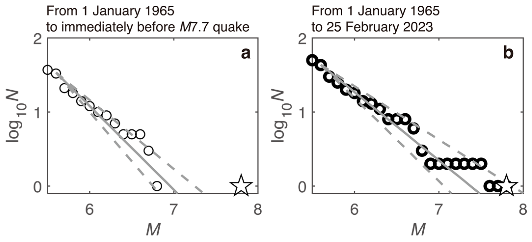
We conducted a simple test to examine whether seismicity along the EAFZ obeys a GR relation or not (Figure 14), where a lower magnitude threshold (M = 5.5) was set to ensure the homogeneity of quake recording since 1965. To create Figure 14, we used the same catalog as that used in Figure 1b,c (see the Data Section). Analysis of the b value [21,22] shows that the M7.7 quake (star) followed the GR trend with b~1 (Figure 14b), indicating that the EAFZ does not have a characteristic magnitude distribution when we used quakes during the period from 1 January 1965 to 25 February 2023. As a reference, we conducted a similar analysis using data before the M7.7 quake. Figure 14a, which indicates the GR distribution with b~1, shows that the M7.7 quake (star) deviates from this distribution. A comparison between these figures (Figure 14a,b) indicates that the M7.7 quake and the following events, including the M7.5 quake, affected the whole magnitude range, such that the M7.7 quake continued to follow the GR trend (Figure 14b). A similar feature was observed for the effect of the 2004 Sumatran megaquake in Indonesia on a global catalog [52]. Our result supports the observation that the M7.7 quake was not an outlier (neither an almighty quake nor a characteristic quake) but was instead harmonized with small quakes along the EAFZ. If an almighty quake or a characteristic quake of the EAFZ existed, it would be much larger than the M7.7 quake.
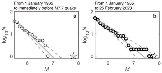
Figure 14.
Cumulative number of quakes as a function of M. (a) Quakes during the period from 1 January 1965 to immediately before the M7.7 quake (the top outside of axes) in the rectangle shown in Figure 1b,c were used. Solid line represents the GR relation with b = 1.13 and a = 7.86. The GR relation, taking the upper and lower bounds (standard deviation) of b values (b = 1.33 and 0.93), is shown by dashed lines. To define the bounds of a b value, we used b values of the bootstrap samples and the computed standard deviations of the sampled b values. Also included for comparison is the M7.7 quake (star), whereas this quake was not included in the data to which the GR relation was fitted. (b) Same as (a) for the period given at the top outside of axes. The GR relation with b = 0.92 ± 0.20 and a = 6.80 is shown by a solid line and dashed lines. The M7.7 quake (star) was included in the data to which the GR relation was fitted.
The feature that the M7.7 quake continued to follow the GR trend (Figure 14b) implies that the underlying mechanism of quake occurrence did not differ from small events to large events. A phenomenon served by the mechanism we focused on is quake clustering, namely seismicity prior and subsequent to the M7.7 quake. Given that this quake and the M7.5 quake that occurred about nine hours later were defined as the doublet quakes, the present paper reported the characteristics of seismicity before and after the doublet quakes. The possibility to analyze the interaction between the doublet quakes was beyond the scope of the present study because several studies [5,6,7,8,9] performed in-depth analyses of it.
7. Conclusions
There are three features of the pre-doublet-quake sequence:
- Seismicity transients began in mid-2022 within 50 km of the future M7.7 epicenter. We revealed that the occurrence rate after mid-2022 was significantly larger than that before it, showing seismic activation. Small b values were observed after the start of activation. The transients reported previously [10,11] were confirmed by our study, which applied the ETAS model and the Bayesian b-value model to events in two different quake catalogs.
- Seismicity within 50 km of the future M7.7 epicenter decomposed into two types of activity: background and clustering. The parameter representing background activity was almost constant over time, while that representing clustering activity was smaller before the start of activation than after it. Seismic activation is interpreted as the effect of clustering activity. This was attributed to the emergence of two clusters near the future M7.7 epicenter [10].
- A high-slip area on the segment (referred to as segment 2 in this study) from which the M7.7 rupture started overlaps with seismicity after the start of activation. This seismicity mostly consisted of events of the cluster displaying low b values. A similar result was observed for the 2011 Tohoku megaquake [30], where a correlation between areas of low b values and areas of large co-seismic displacement was shown. A cluster of high b values that emerged in 2017–2018 overlapped with a low-slip area on the same segment.
There are three features pertaining to seismicity after the doublet quakes:
- Seismicity following the 2020 M6.8 quake suggests that the north end of the M7.7 rupture was close to the south end of the M6.8 rupture. There was a lack of post-M7.5-quake seismic activity at the zone of increase in Coulomb stress imparted by the doublet quakes beyond the north end of the M7.7 rupture, noting that this area, which lacked seismic activity, coincided with the area of the 2020 M6.8 rupture. Our result is consistent with a previous finding [5].
- Locations of the two M6-class quakes around the north and south ends of the M7.7-quake rupture were in relatively high-stress regions compared with the surrounding ones, as implied by the b-value and Coulomb-stress analyses. The region around the hypocenters of the M6-class quakes became closer to failure by the doublet quakes. A similar result was obtained when adding the 2020 M6.8 fault to source faults of Coulomb stress changes.
- The decay of seismic activity with time after the M7.7 quake around the causative faults was well modeled by the standard (single) ETAS model, indicating no pronounced activation or quiescence. This decay also followed the OU relation. Our estimation of the duration of the post-doublet-quake sequence was 1–2 × 10³ days (2.7–5.5 years), a longer duration than that proposed by an earlier study [5]. The difference between the present study and the previous study emerged from the fact that the former used events within 618 days since the M7.7 quake while the latter used events within about 100 days.
Supplementary Materials
The following supporting information can be downloaded at: https://www.mdpi.com/article/10.3390/geosciences15040113/s1, Figure S1: λ, μ, and K0 as a function of time for Mth = 2.0 and 1.5; Figure S2: Map views of b values before the 20 February 2023 M6.4 quake; Figure S3: Same as Figure S2 for Mc; Figure S4: Same as Figure S2, but using the catalog of Lomax [16]; Figure S5: Same as Figure S4 for Mc; Figure S6: Coulomb stress changes; Figure S7: Same as Figure S2, but using quakes during the period from 21 February to immediately before the M5.9 quake; Figure S8: Same as Figure S7 for Mc; Figure S9: Same as Figure S7, but using the catalog of Lomax [16]; Figure S10: Same as Figure S9 for Mc; Figure S11: Same as Figure 12a for M ≥ 3 in a and M ≥ 4 in b; Figure S12: Same as Figure 12b for M ≥ 3 in a and M ≥ 4 in b; Figure S13: Same as Figure 13 for M ≥ 4.5.
Author Contributions
Conceptualization, K.Z.N., J.I., T.H., T.N. and K.O.; methodology, K.Z.N. and T.K.; software, K.Z.N. and T.K.; validation, K.Z.N.; formal analysis, K.Z.N. and T.K.; investigation, K.Z.N. and T.K.; resources, K.Z.N.; data curation, K.Z.N.; writing—original draft preparation, K.Z.N.; writing—review and editing, K.Z.N., T.K., J.I., T.H., T.N. and K.O.; visualization, K.Z.N. and T.K.; supervision, K.Z.N.; project administration, K.Z.N.; funding acquisition, K.Z.N., T.K., J.I., T.H. and T.N. All authors have read and agreed to the published version of the manuscript.
Funding
This study was partially supported by the Ministry of Education, Culture, Sports, Science and Technology (MEXT) of Japan, under The Second Earthquake and Volcano Hazards Observation and Research Program (Earthquake and Volcano Hazard Reduction Research) (K.Z.N., T.K., J.I., and T.N.) and under STAR-E (Seismology TowArd Research innovation with data of Earthquake) Program Grant Number JPJ010217 (K.Z.N. and T.K.), and Collaboration Research Program of IDEAS, Chubu University Grant Number IDEAS202417 (I.J., T.N., and K.Z.N.).
Data Availability Statement
The datasets used in the current study are available from the corresponding author upon reasonable request. The AFAD quake catalog was obtained from https://deprem.afad.gov.tr/event-catalog (accessed on 17 March 2025). The ANSS quake catalog was obtained from https://earthquake.usgs.gov/data/comcat/ (accessed on 17 March 2025). The ISC-GEM quake catalog was obtained from https://doi.org/10.31905/d808b825 (accessed on 17 March 2025). The quake catalog produced by Kwiatek et al. [10] is available as a part of the Supplementary Information of that study. The quake catalog produced by Lomax [16] is available at https://zenodo.org/records/8089273 (accessed on 17 March 2025). The fault models of the 2020 M6.8 quake, the 2023 M7.7 quake, and the 2023 M7.6 quake, which were used in this study, are based on previous work [2,3,4] (https://earthquake.usgs.gov/earthquakes/eventpage/us60007ewc/executive (accessed on 17 March 2025), https://earthquake.usgs.gov/earthquakes/eventpage/us6000jllz/executive (accessed on 17 March 2025), https://earthquake.usgs.gov/earthquakes/eventpage/us6000jlqa/executive (accessed on 17 March 2025)). Moment tensor products of the 1999 M7.6, 1999 M7.2, 2020 M7.0, 2023 M6.4, and 2024 M5.9 quakes [13,14,56,57,58], used for Figure 1a, Figure 8, Figure 10 and Figure S6, is available at https://earthquake.usgs.gov/earthquakes/eventpage/usp0009d4z/executive (accessed on 17 March 2025), https://earthquake.usgs.gov/earthquakes/eventpage/usp0009hev/executive (accessed on 17 March 2025), https://earthquake.usgs.gov/earthquakes/eventpage/us7000c7y0/executive (accessed on 17 March 2025), https://earthquake.usgs.gov/earthquakes/eventpage/us6000jqcn/executive (accessed on 17 March 2025), and https://earthquake.usgs.gov/earthquakes/eventpage/us6000nyzk/executive (accessed on 17 March 2025). The authors digitized plate boundaries [1,59] used for Figure 1a. The time dependence of b shown in Figure 3b of Kwiatek et al. [10] was used to create Figure 2. Active fault data provided by Emre et al. [60] were used. The seismicity analysis software package ZMAP [21], used for computing b values [22] in Figure 9, Figure 11, Figure 14, Figures S2–S5 and S7–S10, and for computing p values in Figure 13 and Figure S13, was obtained from https://github.com/swiss-seismological-service/zmap7 (accessed on 17 March 2025). The graphic-rich deformation and stress-change software Coulomb [33,34], used for Figure 7, Figure 8, Figure 10 and Figure S6, is available for download at https://temblor.net/coulomb/ (accessed on 17 March 2025). The Generic Mapping Tools [61], used for Figure 1, Figure 9, Figure 11, Figures S2–S5 and S7–S10, are an open-source collection (https://www.generic-mapping-tools.org (accessed on 17 March 2025)).
Acknowledgments
We thank the four anonymous reviewers for their constructive comments, and S. Toda and Y. Yamamoto for discussion.
Conflicts of Interest
The authors declare no conflicts of interest.
Abbreviations
The following abbreviations are used in this manuscript:
| AFAD | Disaster and Emergency Management Authority |
| AIC | Akaike Information Criterion |
| ANK | Ankara |
| DSFZ | Dead Sea fault zone |
| EAFZ | East Anatolian fault zone |
| ETAS | Epidemic-Type Aftershock Sequence |
| GR | Gutenberg–Richter |
| HSZ | Hellenic subduction zone |
| IST | Istanbul |
| KHR | Kahramanmaraş |
| KOERI | Kandilli Observatory and Earthquake Research Institute |
| NAFZ | North Anatolian fault zone |
| NAT | North Aegean Trough |
| NP | nodal plane |
| OU | Omori–Utsu |
| USGS | United States Geological Survey |
References
- USGS. The 2023 Kahramanmaraş, Turkey, Earthquake Sequence. 2024. Available online: https://earthquake.usgs.gov/storymap/index-turkey2023.html (accessed on 17 March 2025).
- USGS. M7.8-Pazarcik Earthquake, Kahramanmaras Earthquake Sequence. 2023. Available online: https://earthquake.usgs.gov/earthquakes/eventpage/us6000jllz/executive (accessed on 17 March 2025).
- USGS. M7.5-Elbistan Earthquake, Kahramanmaras Earthquake Sequence. 2023. Available online: https://earthquake.usgs.gov/earthquakes/eventpage/us6000jlqa/executive (accessed on 17 March 2025).
- USGS. M6.7-13 km N of Doğanyol, Turkey. 2020. Available online: https://earthquake.usgs.gov/earthquakes/eventpage/us60007ewc/executive (accessed on 17 March 2025).
- Toda, S.; Stein, R. The role of stress transfer in rupture nucleation and inhibition in the 2023 Kahramanmaraş, Türkiye, sequence, and a one-year earthquake forecast. Seismol. Res. Lett. 2024, 95, 596–606. [Google Scholar] [CrossRef]
- Chen, J.; Liu, C.; Dal Zilio, L.; Cao, J.; Wang, H.; Yang, G.; Göğüş, O.H.; Zhang, H.; Shi, Y. Decoding Stress Patterns of the 2023 Türkiye-Syria Earthquake Doublet. J. Geophys. Res. 2024, 129, e2024JB029213. [Google Scholar] [CrossRef]
- Toda, S.; Stein, R.S.; Özbakir, A.D.; Gonzalez-Huizar, H.; Sevilgen, V.; Lotto, G.; Sevilgen, S. Stress change calculations provide clues to aftershocks in 2023 Türkiye earthquakes. Temblor 2023. [Google Scholar] [CrossRef]
- Kobayashi, T.; Munekane, H.; Kuwahara, M.; Furui, H. Insights on the 2023 Kahramanmaraş Earthquake, Turkey, from InSAR: Fault locations, rupture styles and induced deformation. Geophys. J. Int. 2024, 236, 1068–1088. [Google Scholar] [CrossRef]
- Ren, C.; Wang, Z.; Taymaz, T.; Hu, N.; Luo, H.; Zhao, Z.; Yue, H.; Song, X.; Shen, Z.; Xu, H.; et al. Supershear triggering and cascading fault ruptures of the 2023 Kahramanmaraş, Türkiye, earthquake doublet. Science 2024, 383, 305–311. [Google Scholar] [CrossRef] [PubMed]
- Kwiatek, G.; Martínez-Garzón, P.; Becker, D.; Dresen, G.; Cotton, F.; Beroza, G.C.; Acarel, D.; Ergintav, S.; Bohnhoff, M. Months-long seismicity transients preceding the 2023 MW 7.8 Kahramanmaraş earthquake, Türkiye. Nat. Commun. 2023, 14, 7534. [Google Scholar] [CrossRef]
- Över, S.; Demirci, A.; Özden, S. Tectonic implications of the February 2023 Earthquakes (Mw7.7, 7.6 and 6.3) in south-eastern Türkiye. Tectonophysics 2023, 866, 230058. [Google Scholar] [CrossRef]
- Gutenberg, B.; Richter, C.F. Frequency of earthquakes in California. Bull. Seismol. Soc. Am. 1944, 34, 185–188. [Google Scholar] [CrossRef]
- USGS. M6.3-2 km NNW of Uzunbağ, Turkey. 2023. Available online: https://earthquake.usgs.gov/earthquakes/eventpage/us6000jqcn/executive (accessed on 17 March 2025).
- USGS. M6.0-19 km W of Doğanyol, Turkey. 2024. Available online: https://earthquake.usgs.gov/earthquakes/eventpage/us6000nyzk/executive (accessed on 17 March 2025).
- Utsu, T. A statistical study on the occurrence of aftershocks. Geophys. Mag. 1961, 30, 521–605. [Google Scholar]
- Lomax, A. Precise, NLL-SSST-Coherence Hypocenter Catalog for the 2023 Mw 7.8 and Mw 7.6 SE Turkey Earthquake Sequence. 2023. Available online: https://zenodo.org/records/8089273 (accessed on 17 March 2025).
- Ogata, Y. Statistical models for earthquake occurrences and residual analysis for point processes. J. Am. Stat. Assoc. 1988, 83, 9–27. [Google Scholar] [CrossRef]
- Dieterich, J. A constitutive law for rate of earthquake production and its application to earthquake clustering. J. Geophys. Res. 1994, 99, 2601–2618. [Google Scholar] [CrossRef]
- Akaike, H. A new look at the statistical model identification. IEEE Trans. Autom. Control 1974, 19, 716–723. [Google Scholar] [CrossRef]
- Ogata, Y.; Tsuruoka, H. Statistical monitoring of aftershock sequences: A case study of the 2015 Mw7.8 Gorkha, Nepal, earthquake. Earth Planets Space 2016, 68, 44. [Google Scholar] [CrossRef]
- Wiemer, S. A software package to analyze seismicity: ZMAP. Seismol. Res. Lett. 2012, 72, 373–382. [Google Scholar] [CrossRef]
- Woessner, J.; Wiemer, S. Assessing the quality of earthquake catalogues: Estimating the magnitude of completeness and its uncertainty. Bull. Seismol. Soc. Am. 2005, 95, 684–698. [Google Scholar] [CrossRef]
- Nanjo, K.Z.; Yoshida, A. A b map implying the first eastern rupture of the Nankai Trough earthquakes. Nat. Commun. 2018, 9, 1117. [Google Scholar] [CrossRef] [PubMed]
- Kumazawa, T.; Ogata, Y.; Tsuruoka, H. Characteristics of seismic activity before and after the 2018 M6.7 Hokkaido Eastern Iburi earthquake. Earth Planets Space 2019, 71, 130. [Google Scholar] [CrossRef]
- Nanjo, K.Z. Were changes in stress state responsible for the 2019 Ridgecrest, California, earthquakes? Nat. Commun. 2020, 11, 3082. [Google Scholar] [CrossRef]
- Scholz, C.H. The frequency-magnitude relation of microfracturing in rock and its relation to earthquakes. Bull. Seismol. Soc. Am. 1968, 58, 399–415. [Google Scholar] [CrossRef]
- Lei, X. How do asperities fracture? An experimental study of unbroken asperities. Earth Planet. Sci. Lett. 2003, 213, 347–359. [Google Scholar] [CrossRef]
- Goebel, T.H.W.; Schorlemmer, D.; Becker, T.W.; Dresen, G.; Sammis, C.G. Acoustic emissions document stress changes over many seismic cycles in stick-slip experiments. Geophys. Res. Lett. 2013, 40, 2049–2054. [Google Scholar] [CrossRef]
- Tormann, T.; Enescu, B.; Woessner, J.; Wiemer, S. Randomness of megathrust earthquakes implied by rapid stress recovery after the Japan earthquake. Nat. Geosci. 2015, 8, 152–158. [Google Scholar] [CrossRef]
- Nanjo, K.Z.; Hirata, N.; Obara, K.; Kasahara, K. Decade-scale decrease in b value prior to the M9-class 2011 Tohoku and 2004 Sumatra quakes. Geophys. Res. Lett. 2012, 39, L20304. [Google Scholar] [CrossRef]
- Schurr, B.; Asch, G.; Hainzl, S.; Bedford, J.; Hoechner, A.; Palo, M.; Wang, R.; Moreno, M.; Bartsch, M.; Zhang, Y.; et al. Gradual unlocking of plate boundary controlled initiation of the 2014 Iquique earthquake. Nature 2014, 512, 299–302. [Google Scholar] [CrossRef]
- Ito, R.; Kaneko, Y. Physical mechanism for a temporal decrease of the Gutenberg-Richter b-value prior to a large earthquake. J. Geophys. Res. 2023, 128, e2023JB027413. [Google Scholar] [CrossRef]
- Lin, J.; Stein, R.S. Stress triggering in thrust and subduction earthquakes, and stress interaction between the southern San Andreas and nearby thrust and strike-slip faults. J. Geophys. Res. 2024, 109, B02303. [Google Scholar] [CrossRef]
- Toda, S.; Stein, R.S.; Richards-Dinger, K.; Bozkurt, S. Forecasting the evolution of seismicity in southern California: Animations built on earthquake stress transfer. J. Geophys. Res. 2005, 110, B05S16. [Google Scholar] [CrossRef]
- Storchak, D.A.; Di Giacomo, D.; Bondár, I.; Engdahl, E.R.; Harris, J.; Lee, W.H.K.; Villaseñor, A.; Bormann, P. Public release of the ISC-GEM Global Instrumental Earthquake Catalogue (1900–2009). Seismol. Res. Lett. 2013, 84, 810–815. [Google Scholar] [CrossRef]
- Storchak, D.A.; Di Giacomo, D.; Engdahl, E.R.; Harris, J.; Bondár, I.; Lee, W.H.K.; Bormann, P.; Villaseñor, A. The ISC-GEM Global Instrumental Earthquake Catalogue (1900–2009): Introduction. Phys. Earth Planet. Inter. 2015, 239, 48–63. [Google Scholar] [CrossRef]
- Di Giacomo, D.; Engdahl, E.R.; Storchak, D.A. The ISC-GEM Earthquake Catalogue (1904–2014): Status after the Extension Project. Earth Syst. Sci. Data 2018, 10, 1877–1899. [Google Scholar] [CrossRef]
- International Seismological Centre. ISC-GEM Earthquake Catalogue; International Seismological Centre: Berkshire, UK, 2022. [Google Scholar] [CrossRef]
- USGS Earthquake Hazards Program. Advanced National Seismic System (ANSS) Comprehensive Catalog of Earthquake Events and Products: Various; USGS: Reston, VA, USA, 2017. [CrossRef]
- Lomax, A.; Savvaidis, A. High-precision earthquake location using source-specific station terms and inter-event waveform similarity. J. Geophys. Res. 2022, 127, e2021JB023190. [Google Scholar] [CrossRef]
- Lomax, A.; Henry, P. Major California faults are smooth across multiple scales at seismogenic depth. Seismica 2023, 2, 108145. [Google Scholar] [CrossRef]
- Melgar, D.; Taymaz, T.; Ganas, A.; Crowell, B.W.; Öcalan, T.; Kahraman, M.; Tsironi, V.; Yolsal-Çevikbil, S.; Valkaniotis, S.; Irmak, T.S.; et al. Sub- and super-shear ruptures during the 2023 Mw 7.8 and Mw 7.6 earthquake doublet in SE Türkiye. Seismica 2023, 2, 1–10. [Google Scholar] [CrossRef]
- van der Elst, N.J. B-positive: A robust estimator of aftershock magnitude distribution in transiently incomplete catalogs. J. Geophys. Res. 2021, 126, e2020JB021027. [Google Scholar] [CrossRef]
- Lippiello, E.; Petrillo, G. B-more-incomplete and b-more-positive: Insights on a robust estimator of magnitude distribution. J. Geophys. Res. 2024, 129, e2023JB027849. [Google Scholar] [CrossRef]
- Iwata, D.; Nanjo, K.Z. Adaptive estimation of the Gutenberg–Richter b value using a state space model and particle filtering. Sci. Rep. 2024, 14, 4630. [Google Scholar] [CrossRef] [PubMed]
- Kumazawa, T.; Ogata, Y.; Tsuruoka, H. Measuring seismicity diversity and anomalies by point process models: Case studies before and after the 2016 Kumamoto Earthquakes in Kyushu, Japan. Earth Planets Space 2017, 69, 169. [Google Scholar] [CrossRef]
- Nanjo, K.Z.; Yukutake, Y.; Kumazawa, T. Activated volcanism of Mount Fuji by the 2011 Japanese large earthquakes. Sci. Rep. 2023, 13, 10562. [Google Scholar] [CrossRef]
- Ogata, Y. Detection of precursory relative quiescence before great earthquakes through a statistical model. J. Geophys. Res. 1992, 97, 19845–19871. [Google Scholar] [CrossRef]
- Kumazawa, T.; Ogata, Y. Quantitative description of induced seismic activity before and after the 2011 Tohoku-Oki Earthquake by non-stationary ETAS models. J. Geophys. Res. 2013, 118, 6165–6182. [Google Scholar] [CrossRef]
- Kumazawa, T.; Ogata, Y.; Kimura, K.; Maeda, K.; Kobayashi, A. Background rates of swarm earthquakes that are synchronized with volumetric strain changes. Earth Planet. Sci. Lett. 2016, 442, 51–60. [Google Scholar] [CrossRef]
- Schorlemmer, D.; Wiemer, S.; Wyss, M. Earthquake statistics at Parkfield: 1. Stationarity of b values. J. Geophys. Res. 2024, 109, B12307. [Google Scholar] [CrossRef]
- Main, I.; Li, L.; McCloskey, J.; Naylor, M. Effect of the Sumatran mega-earthquake on the global magnitude cut-off and event rate. Nat. Geosci. 2008, 1, 142. [Google Scholar] [CrossRef]
- Parsons, T.; Geist, E.L.; Console, R.; Carluccio, R. Characteristic earthquake magnitude frequency distributions on faults calculated from consensus data in California. J. Geophys. Res. 2018, 123, 10761–10784. [Google Scholar] [CrossRef]
- Schwartz, D.P.; Coppersmith, K.J. Fault behavior and characteristic earthquakes: Examples from Wasatch and San Andreas fault zones. J. Geophys. Res. 1984, 89, 5681–5698. [Google Scholar] [CrossRef]
- Shimazaki, K. The almighty earthquake. Seismol. Res. Lett. 1999, 70, 147–148. [Google Scholar] [CrossRef]
- USGS. M7.2-8 km S of Düzce, Turkey. 1999. Available online: https://earthquake.usgs.gov/earthquakes/eventpage/usp0009hev/executive (accessed on 17 March 2025).
- USGS. M7.6-4 km ESE of Derince, Turkey. 1999. Available online: https://earthquake.usgs.gov/earthquakes/eventpage/usp0009d4z/executive (accessed on 17 March 2025).
- USGS. M7.0-13 km NNE of Néon Karlovásion, Greece. 2020. Available online: https://earthquake.usgs.gov/earthquakes/eventpage/us7000c7y0/executive (accessed on 17 March 2025).
- Lazos, I.; Sboras, S.; Pikridas, C. Tectonic geodesy synthesis and review of the North Aegean region, based on the strain patterns of the North Aegean Sea, Strymon basin and Thessalian basin case studies. Appl. Sci. 2023, 13, 9943. [Google Scholar] [CrossRef]
- Emre, Ö.; Duman, T.Y.; Olgun, S.; Elmaci, H.; Özalp, S. 1:250,000 Scale Active Fault Map Series of Turkey, Gaziantep (NJ 37-9) Quadrangle; General Directorate of Mineral Research and Exploration: Ankara, Turkey, 2012.
- Wessel, P.; Smith, W.H.F.; Scharroo, R.; Luis, J.F.; Wobbe, F. Generic Mapping Tools: Improved version released. EOS Trans. AGU 2013, 94, 409–410. [Google Scholar] [CrossRef]

Disclaimer/Publisher’s Note: The statements, opinions and data contained in all publications are solely those of the individual author(s) and contributor(s) and not of MDPI and/or the editor(s). MDPI and/or the editor(s) disclaim responsibility for any injury to people or property resulting from any ideas, methods, instructions or products referred to in the content. |
© 2025 by the authors. Licensee MDPI, Basel, Switzerland. This article is an open access article distributed under the terms and conditions of the Creative Commons Attribution (CC BY) license (https://creativecommons.org/licenses/by/4.0/).