GIS-Based Landslide Susceptibility Mapping with a Blended Ensemble Model and Key Influencing Factors in Sentani, Papua, Indonesia

Abstract

Landslides represent a recurrent hazard in tropical mountain environments, where rapid urbanization and extreme rainfall amplify disaster risk. The Sentani region of Papua, Indonesia, is highly vulnerable, as demonstrated by the catastrophic debris flows of March 2019 that caused fatalities and widespread losses. This study developed high-resolution landslide susceptibility maps for Sentani using an ensemble machine learning framework. Three base learners—Random Forest, eXtreme Gradient Boosting (XGBoost), and CatBoost—were combined through a logistic regression meta-learner. Predictor redundancy was controlled using Pearson correlation and Variance Inflation Factor/Tolerance (VIF/TOL). The landslide inventory was constructed from multitemporal satellite imagery, integrating geological, topographic, hydrological, environmental, and seismic factors. Results showed that lithology, Slope Length and Steepness Factor (LS Factor), and earthquake density consistently dominated model predictions. The ensemble achieved the most balanced predictive performance, Area Under the Curve (AUC) > 0.96, and generated susceptibility maps that aligned closely with observed landslide occurrences. SHapley Additive Explanations (SHAP) analyses provided transparent, case-specific insights into the directional influence of key factors. Collectively, the findings highlight both the robustness and interpretability of ensemble learning for landslide susceptibility mapping, offering actionable evidence to support disaster preparedness, land-use planning, and sustainable development in Papua.

1. Introduction

Landslides and debris flows are among the most widespread and destructive geohazards, particularly in mountainous regions where steep slopes store large volumes of unconsolidated material that can be rapidly mobilized during episodes of intense rainfall [1,2,3,4]. Once triggered, these masses often move downslope and accumulate in valley bottoms or on alluvial fans. Alluvial fans are commonly used for settlement because they are gently sloping, well-drained, elevated above major river flood levels, and often offer favorable views. However, they are inherently prone to torrential hazards—a spectrum of high-energy water-sediment flows that includes debris flows, debris floods, hyperconcentrated flows, and flash floods—which can entrain boulders and woody debris, damaging any part of a fan surface [5]. Consequently, communities on such landforms remain highly exposed to debris flow impacts.

Historical disasters in Asia and South America have repeatedly shown that densely populated alluvial fans are highly vulnerable, with debris flow events resulting in significant casualties and severe economic losses [6,7,8]. Globally, between 2004 and 2016 alone, more than 4800 non-seismic landslide events caused approximately 56,000 fatalities and direct economic losses exceeding USD 2.7 billion [9]. These statistics underscore landslides as a major global challenge, highlighting the urgent need for systematic assessment and proactive risk mitigation strategies.

The Sentani region of Papua, Indonesia, represents a highly relevant local context within this global problem. On 16 March 2019, extreme rainfall triggered catastrophic debris flows from the Cyclops Mountains, resulting in 112 fatalities, the displacement of more than 11,000 residents, and an estimated USD 31.5 million in losses. Most of the devastation occurred in rapidly expanding settlements located on lowland alluvial fans, including residential areas such as Doyo Baru Residence in Sentani, which were directly struck by debris flows [10]. The March 2019 event produced widespread landslides across the Cyclops range, where sediment from slope failures was transported downslope and deposited in lower-slope areas and river channels, particularly in the Kemiri, Doyo, and Sereh watersheds (Figure 1) [11,12]. This disaster emphasized how unregulated settlement expansion into hazard-prone landforms amplifies disaster impacts and highlighted the necessity of reliable landslide susceptibility mapping (LSM) to inform preparedness and spatial planning in Papua.

In this study, we focus on LSM, which provides a spatial representation of areas more prone to slope failures [13,14]. Landslide susceptibility refers to the likelihood of a terrain experiencing landslides given its physical and environmental conditions, without considering the timing of occurrence. It is typically derived from factors such as topography, geology, rainfall, and land use, and is generally considered static over a given period [13,14]. Unlike hazard or risk assessments that also account for temporal probability, intensity, and potential losses, susceptibility analysis emphasizes the spatial dimension of terrain predisposition.

In this study, we apply an integrated approach to the Sentani region that combines geological, topographic, geomorphological, hydrological, environmental, and seismological information derived from geospatial datasets. A key input is the landslide inventory, which was developed through the interpretation of multitemporal satellite imagery to capture both pre- and post-event slope failures [15]. Remote sensing plays a central role in this process, as it allows systematic detection of new landslides and continuous updates of the inventory, which are essential for understanding hazard dynamics and supporting long-term risk reduction [15].

Building on this foundation, we explore the use of advanced machine learning techniques—Random Forest (RF) [16], eXtreme Gradient Boosting (XGBoost) [17], and CatBoost [18]—as base learners, which are subsequently combined through an ensemble meta-learning strategy to further enhance predictive performance [19,20]. The aim of this study is to generate high-resolution susceptibility maps that deliver spatial insights to support disaster preparedness, inform land-use planning, and contribute to sustainable development in Papua. This is particularly urgent in the Sentani region, where rapid urban expansion, rugged mountainous terrain, and recurrent extreme rainfall events have combined to elevate landslide risk in recent years. By advancing data-driven approaches for susceptibility assessment, this study seeks not only to improve predictive accuracy but also to provide actionable knowledge for reducing disaster risk in one of Indonesia’s most hazard-prone environments.

Figure 1. (a) Distribution of landslides and sediment from the Cyclops Mountains toward the Doyo Baru area, derived from Sentinel-2 imagery [21]. Sediment from slope failures was transported and deposited in lower-slope areas and river channels. (b) Damaged houses buried by debris in Doyo Baru [22]. (c) Aerial view of debris flow deposits affecting settlements on the alluvial fan in Sentani [23].

Figure 1. (a) Distribution of landslides and sediment from the Cyclops Mountains toward the Doyo Baru area, derived from Sentinel-2 imagery [21]. Sediment from slope failures was transported and deposited in lower-slope areas and river channels. (b) Damaged houses buried by debris in Doyo Baru [22]. (c) Aerial view of debris flow deposits affecting settlements on the alluvial fan in Sentani [23].

2. Materials and Methods

2.1. Study Area

The Cyclops Mountains are situated west of Jayapura and north of Lake Sentani in Papua Province, Indonesia, spanning ~36 km east–west and ~6 km north–south at the 200 m contour. Rising steeply from the coast, the range reaches over 2000 m a.s.l., while Sentani town at the foothills lies at ~94 m a.s.l. [24]. Designated as a nature reserve in 1978 (re-affirmed in 1995), the protected area covers ~31,400 ha (314 km²), making it one of the largest tropical montane forest reserves adjacent to an urban center in Papua [24].

The region experiences a humid tropical climate, with annual rainfall ranging from ~1500 mm on the southern slopes and nearly 3900 mm on the north coast [24]. Rainfall peaks between December and April, with drier months from May to November, although water scarcity is common during the dry season. Vegetation varies strongly with elevation, the lowland forests occupy elevations less than 600 m, and montane forests dominate at elevations over 1000 m [24]. Ecologically, the reserve protects both primary and secondary forests, serving as the main freshwater source for the Sentani region and supporting high biodiversity and endemism [25].

The study area is situated in the Cyclops Mountains of northeastern Papua, Indonesia, encompassing Lake Sentani and the city of Jayapura (Figure 2a). Geologically, the range is dominated by the Cyclops Metamorphic Complex (pTmc)—comprising schist, gneiss, phyllite, amphibolite, unakite, marble, and hornfels—and ultramafic rocks (um), including harzburgite, serpentinite, pyroxenite, and dunite, which represent the oldest lithologies in the region [26]. These rocks formed through regional metamorphism and subduction-related processes, with serpentinite derived from hydration of peridotites. Structurally, the mountains display a complex tectonic setting of anticlines, synclines, normal, thrust, and strike-slip faults, with dominant orientations trending east–west and northeast–southwest [26]. A major thrust fault separates the metamorphic and ultramafic units, while northeast–southwest strike-slip faults offset earlier structures and frequently define contacts with younger sedimentary units, particularly the Nubai Formation (Tomn) consisting of limestone, sandstone, and marl. This structural and lithological configuration reflects a long tectonic history of subduction, volcanism, and uplift from the Cretaceous to Early Miocene, when submarine volcanism formed the Auwewa Formation (Tcma) and subsequent uplift during the Oligocene exposed metamorphic and ultramafic complexes [26]. The result is a highly deformed and tectonically active mountain belt with significant implications for seismicity and geomorphic hazards.

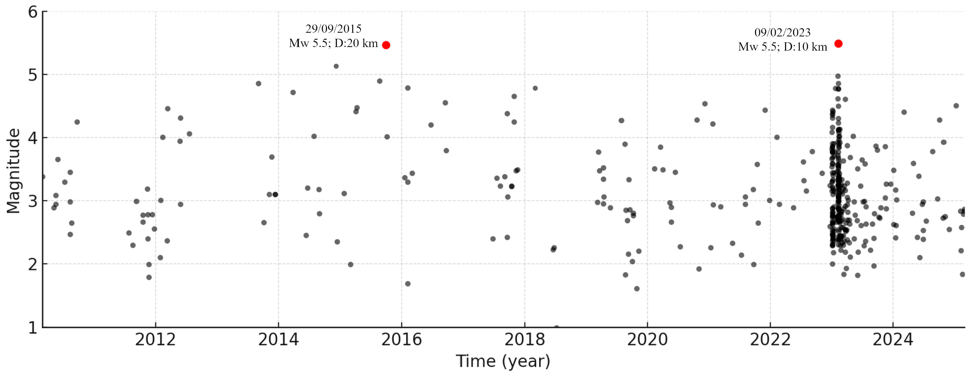
Seismic records from Incorporated Research Institution for Seismology (IRIS) and the Indonesian Meteorology, Climatology, and Geophysical Agency (BMKG) catalogs (2000–2024) reported 412 earthquakes concentrated along the fault zones around Lake Sentani and Jayapura (Figure 2b) [27,28]. These events cluster along mapped structural lineaments, with the largest earthquakes (Mw 5.5) occurring near Jayapura in September 2015 (20 km depth) and February 2023 (10 km depth). Shallow seismicity (5–20 km depth) is particularly prevalent near Jayapura and the eastern margin of Lake Sentani. Temporally, seismicity between 2000 and 2021 was scattered, with magnitudes mostly Mw 2–4 and few moderate events, but a marked increase occurred in late 2022, culminating in a seismic swarm in early 2023 (Figure 3). This clustering suggests reactivation of local fault systems or stress accumulation along lithological boundaries.

2.2. Input Data

This study established a spatial database within a Geographic Information System (GIS) environment, consisting of a landslide inventory map and ten thematic factor maps derived from topographic, geological, hydrological, environmental, and seismological datasets (

Table 1. Summary of datasets used in the study, including sources, formats, resolutions, and derived factors.

No	Data Name	Data Source	Spatial Resolution	Data Type	Derivative Maps
1	Digital Elevation Model (DEM)	Ina-Geoportal, Geospatial Information Agency of Indonesia [29]	8.3 m × 8.3 m	Raster grid	Elevation, Slope, Aspect, Curvature, Terrain Ruggedness Index (TRI), Slope Length Factor (LS Factor); Geomorphic units, Stream Power Index (SPI); Distance to river, River density, Topographic Wetness Index (TWI), Total Catchment Area (TCA)
2	Geological Map	Geological Map of the Jayapura (Cyclops Mountains) Quadrangle, Irian Jaya, Scale 1:100,000 [26]	1:100,000 scale	Document	Lithology, Distance to fault, Fault density
3	Sentinel-2A Satellite Imagery	Copernicus Open Access Hub [21]	10 m × 10 m	Raster grid	Normalized Difference Vegetation Index (NDVI); Normalized Difference Water Index (NDWI)
4	Soil Map	SoilGrids by ISRIC—World Soil Information [30]	250 m × 250 m	Raster grid	Soil type
5	Land Use Map	ESA WorldCover 2021 V200, European Space Agency [31]	10 m × 10 m	Raster grid	Land use
6	Earthquake Catalog	Incorporated Research Institutions for Seismology (IRIS) [27] and BMKG [28]	Point-based; no fixed resolution	Vector shapefile (point)	Earthquake event density

).

2.2.1. Landslide Inventory Map

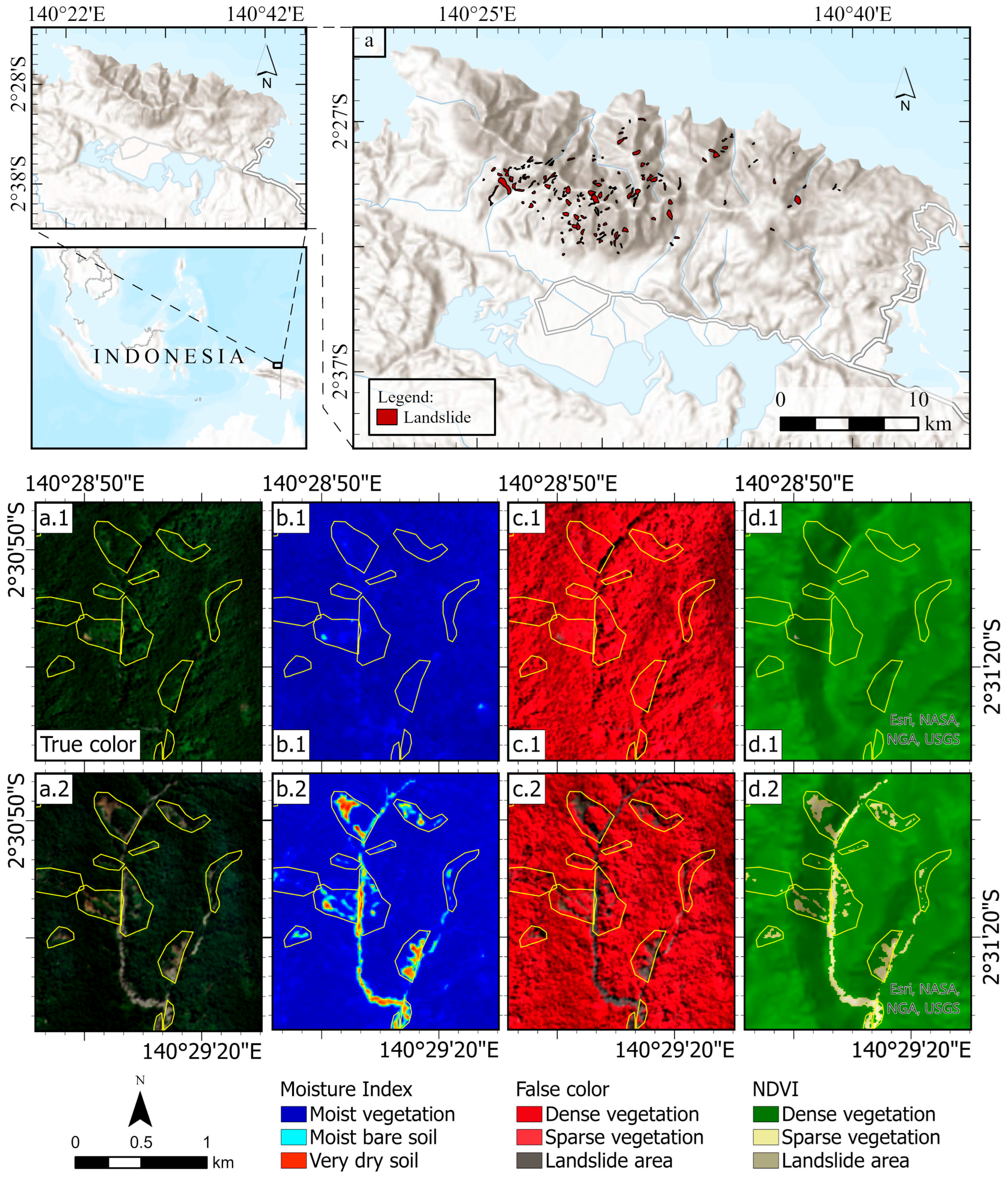
The landslide inventory map of the Cyclops Mountains (Figure 4) was generated from multi-temporal Sentinel-2A imagery (2015–2025) using semi-automatic visual interpretation. A total of 177 landslides were delineated. Figure 4 illustrates both the spatial distribution of mapped landslides and the spectral analyses (true color, moisture index, false color, and NDVI) applied to support the identification of scarps, exposed soils, and vegetation loss. The resulting inventory formed the basis for sampling and subsequent validation of the susceptibility models.

2.2.2. Landslide Factors

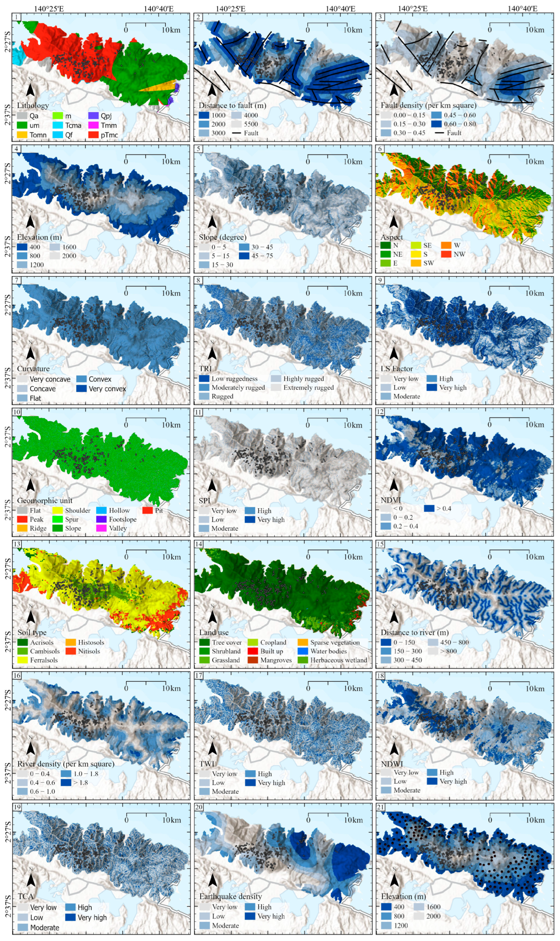
To identify the most relevant contributing factors for landslide susceptibility, this study selected 20 conditioning variables derived from geological, topographic, geomorphological, environmental, hydrological, and seismological datasets. The selection was based on their theoretical relevance and support from previous studies. These factors were processed in a GIS environment to produce thematic layers for use in the susceptibility modeling, namely:

Lithology

Lithology plays a key role in landslide processes through its properties such as permeability, porosity, and rock or soil strength. Different lithological units show varying levels of susceptibility to slope failure. In this study, the lithological map of the Cyclops Mountains was compiled from the official 1:100,000 Geological Map of Jayapura Quadrangle [26], which was digitized and analyzed. The main lithological units include pre-Tertiary metamorphic rocks (pTmc) and ultramafic rocks (um), Tertiary sedimentary and volcanic rocks (Tcma, Tomn, Tmm), and Quaternary deposits such as alluvium (Qa) and fan deposits (Qf) (Figure 5(1)).

Distance to Fault

The Euclidean distance to the nearest fault line was generated from the geological map to evaluate the influence of tectonic structures on slope instability (Figure 5(2)). Euclidean distance refers to the straight-line distance between a location and the closest fault, making it a simple yet effective way to quantify spatial proximity. Proximity to fault lines is considered a critical factor, as active or inactive faults can weaken rock masses and increase susceptibility to ground movement triggered by seismic or non-seismic processes [32]. Areas closer to major faults generally show a higher concentration of landslides, reflecting the structural control on terrain degradation.

Fault Density

In addition to fault distance, a fault density layer was derived using a 1-km² circular moving window (Figure 5(3)). This parameter represents the spatial intensity of fault networks and their potential cumulative effect on slope failure. Regions with high fault density tend to exhibit greater rock mass fragmentation and higher seismic influence, resulting in elevated landslide occurrence [33]. The combined use of fault distance and density provides a more comprehensive assessment of tectonic contributions to slope instability.

Elevation

Elevation affects climate and hydrological patterns, influencing rainfall distribution, vegetation cover, and soil development (Figure 5(4)) [34]. In mountainous regions, higher elevation zones tend to receive more precipitation due to orographic effects, while lower areas remain relatively drier. Generally, as elevation increases, slope processes become more dynamic, leading to a higher likelihood of landslide occurrence.

Slope

Slope is a fundamental topographic parameter derived from the Digital Elevation Model (DEM) (Figure 5(5)). It describes the rate of elevation change and provides insight into terrain steepness and energy [35]. Steeper slopes often influence surface runoff, soil redistribution, and hydrological pathways. In this study, the slope layer was calculated using standard terrain analysis tools and resampled to match the resolution of other conditioning factors. The resulting dataset represents spatial variability in terrain gradients across the study area and is further integrated into the susceptibility modeling framework.

Aspect

Aspect categorized into eight directions, influences solar radiation, evapotranspiration, and soil moisture, thereby affecting vegetation stability and microclimatic conditions (Figure 5(6)). Slopes facing east and west may experience higher temperature fluctuations, while north- and south-facing slopes differ in terms of moisture retention and vegetation density. These variations play an important role in slope stability, as drier slopes are often more susceptible to shallow landslides compared to shaded, moisture-rich aspects [36].

Curvature

Curvature describes surface shape—concave, convex, or flat—affecting water flow and sediment accumulation on slopes (Figure 5(7)). Concave slopes tend to concentrate water and promote soil saturation, increasing the likelihood of slope failure. In contrast, convex slopes encourage runoff and erosion, while flat areas act as deposition zones. This makes curvature an essential factor for identifying slope segments vulnerable to erosion or landslides [37].

The Terrain Ruggedness Index (TRI)

TRI quantifies surface roughness and highlights areas with abrupt elevation changes, which are often associated with unstable terrain [38] (Figure 5(8)). High TRI values typically correspond to rugged landscapes, where landslides are more frequent. In the Cyclops Mountains, zones with high TRI coincide with steep cliffs and dissected valleys, indicating a strong geomorphic control on slope instability.

Slope Length and Steepness Factor (LS Factor)

The LS factor, derived from the Revised Universal Soil Loss Equation (RUSLE), integrates slope gradient and flow length to quantify soil erosion (Figure 5(9)). RUSLE is an empirical model widely applied in hydrology and geomorphology to estimate average annual soil loss by considering rainfall, soil type, topography, land cover, and conservation practices [39]. Long slopes with high steepness increase runoff velocity, which enhances soil detachment and sediment delivery downslope. In mountainous regions such as the Cyclops Mountains, high LS values are strongly associated with gully formation, surface erosion, and the initiation of debris flows.

Geomorphic Units

Geomorphic units were derived using the Topographic Position Index (TPI), which classifies the landscape into peaks, ridges, slopes, flats, footslopes, valleys, and hollows (Figure 5(10)). These landform types are useful for identifying slope conditions that control runoff, soil erosion, and mass movement processes [40]. Steep slopes, ridges, and hollows are particularly critical, as they are often associated with higher landslide susceptibility due to concentrated stresses and water accumulation.

Stream Power Index (SPI)

SPI measures the erosive capacity of flowing water by combining slope and upstream contributing area (Figure 5(11)). High SPI values indicate zones of concentrated flow that can intensify incision, slope undercutting, and sediment mobilization [41]. In mountainous terrain, such areas are critical in triggering debris flows and accelerating slope instability.

Normalized Difference Vegetation Index (NDVI)

NDVI was derived from Sentinel-2A imagery using the red and near-infrared bands (Figure 5(12)). NDVI reflects vegetation health and density, where low values indicate bare or disturbed surfaces. Such variations in vegetation cover can influence surface conditions relevant to slope stability [42].

Soil type

Soil data were obtained from the SoilGrids dataset and resampled to match other spatial layers [30]. The main soil groups include Acrisols, Cambisols, Ferralsols, Histosols, and Nitisols, each characterized by varying permeability, cohesiveness, and moisture retention properties (Figure 5(13)). These differences can influence how soils interact with water and surface processes.

Land use

Land use and cover information was extracted from ESA WorldCover 2021, which categorizes the area into tree cover, agriculture, shrubland, grassland, urban zones, wetlands, mangroves, and water bodies (Figure 5(14)) [31]. Changes in land use, such as deforestation or urban expansion, alter vegetation distribution and surface characteristics, which may affect hydrological and geomorphological dynamics.

Distance to river

The Euclidean distance to rivers was derived from a hydrologically corrected stream network (Figure 5(15)). This layer represents proximity to drainage channels, which can influence soil moisture conditions and patterns of riverbank erosion, especially in steep terrain.

River density

River density was calculated as the total stream length within a given area (Figure 5(16)). Higher values reflect a denser drainage network, which may affect surface runoff distribution and the overall connectivity of water flow.

Topographic Wetness Index (TWI)

TWI quantifies the spatial distribution of soil moisture based on slope and contributing area (Figure 5(17)) [38,41]. Higher index values generally indicate locations with greater potential for water accumulation.

Normalized Difference Water Index (NDWI)

NDWI derived from Sentinel-2 imagery, highlights regions with elevated surface moisture or standing water [43]. This index is useful for identifying hydrological conditions across the landscape (Figure 5(18)).

Total Catchment Area (TCA)

TCA represents the area that drains into a specific location, describing the potential water contribution from upslope regions [44]. Larger contributing areas indicated higher flow accumulation (Figure 5(19)).

Earthquake Density

Earthquake density was developed from seismic data provided by the Indonesian Meteorology, Climatology, and Geophysical Agency (BMKG) [28] and IRIS [27] between 2000 and 2024 (Figure 5(20)). The dataset included shallow and moderate-to-strong events, interpolated to highlight spatial clustering of seismic activity. This layer was incorporated to represent tectonic influences within the study area.

2.2.3. Dataset and Sampling

A dataset was constructed comprising 177 landslide points (positive class) derived from landslide inventory map and 177 non-landslide points (negative class) randomly sampled outside a 1 km buffer from known landslides to reduce spatial autocorrelation and sampling bias [45,46,47]. This buffer-based exclusion ensures spatial independence between classes and prevents contamination during model training. The final dataset of 354 points was randomly split into 80% for training (284 samples) and 20% for validation (70 samples), supporting robust model evaluation and generalization. Figure 5(21) illustrates the spatial distribution of landslide (black) and non-landslide (red) points overlaid on an elevation background.

2.3. Method

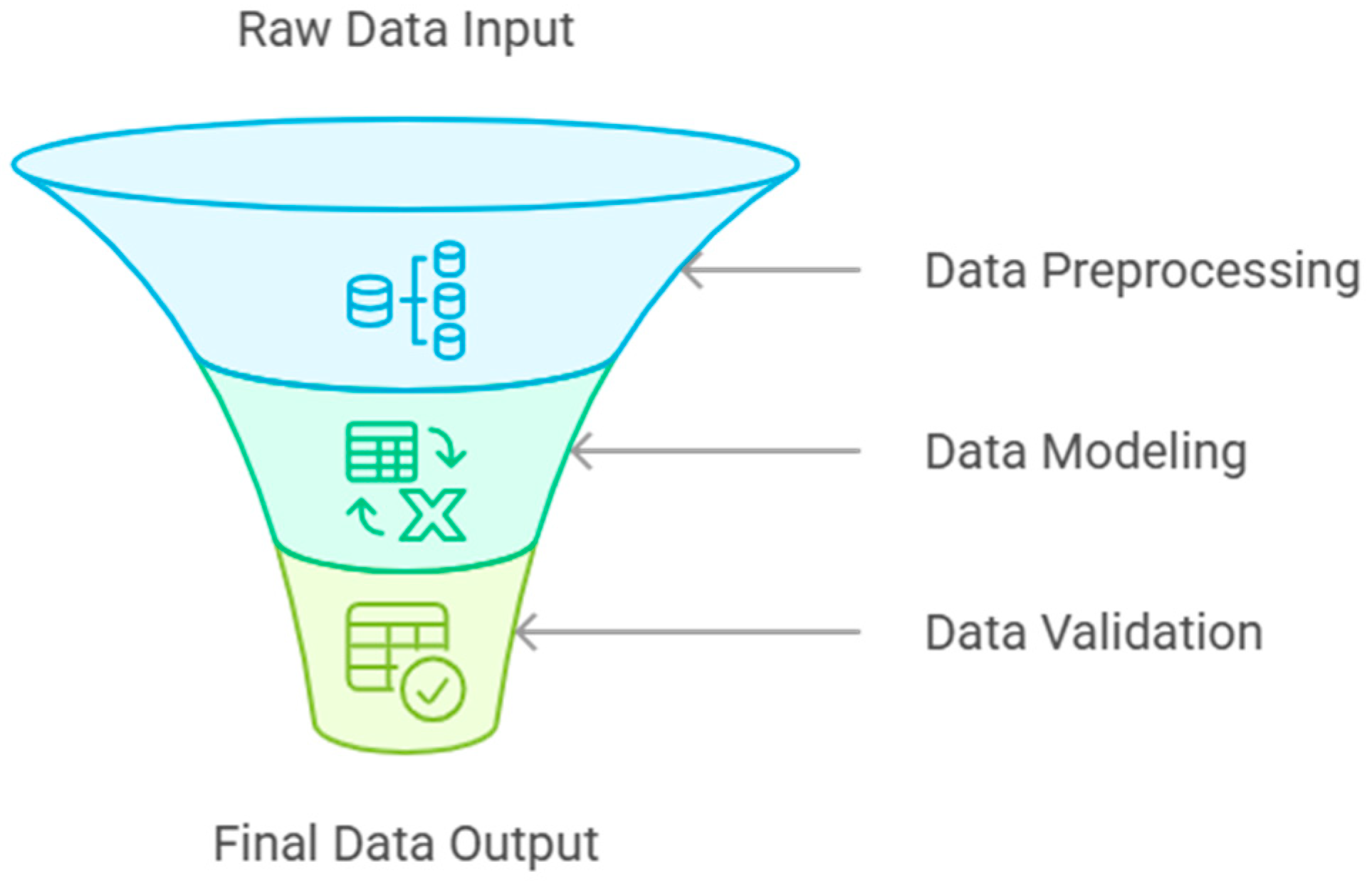
The methodological framework applied in this study follows a structured five-stage workflow, illustrated in Figure 6. Each stage is interconnected, ensuring consistency from data preparation to spatial prediction.

2.3.1. Data Input

The first step integrates multi-source datasets essential for susceptibility modeling. The landslide inventory was compiled from historical records and remote sensing, while nineteen conditioning factors were derived from geological, geomorphological, hydrological, seismic, and environmental data sources. These factors include lithology, slope, curvature, NDVI, NDWI, river density, distance to rivers, earthquake density, and others, all of which were prepared in raster format. A separate dataset of historical landslides was used for spatial validation.

In this stage, it is crucial to ensure that all spatial datasets are standardized before further analysis [48,49]. Specifically, all raster layers were projected to the same coordinate reference system (CRS), in this case UTM Zone 54S, which corresponds to the Sentani study area in Papua, Indonesia. Moreover, all layers were resampled to a consistent spatial resolution and clipped to the same geographic extent, resulting in rasters with identical numbers of rows and columns. This harmonization ensures pixel-level correspondence across all conditioning factors [50]. To ensure that the coding workflow operates properly, this preprocessing step is essential. By preparing all spatial data in a uniform CRS, resolution, and extent, the raster stack can be read consistently, enabling reliable and reproducible susceptibility modeling.

2.3.2. Preprocessing

The preprocessing stage involved several key steps, including data cleaning, normalization, and the assessment of multicollinearity [51]. Attribute names were standardized, and redundant features were screened using Pearson correlation and Variance Inflation Factor (VIF)/Tolerance (TOL). To ensure comparability among predictors, a Min–Max normalization was applied, transforming all values into the range [0, 1]. Finally, the dataset was randomly split into 80% sub-training and 20% validation, with stratification applied to preserve the class balance between landslide and non-landslide samples.

Pearson correlation is a statistical measure that quantifies the linear relationship between two continuous variables, ranging from –1 (perfect negative correlation) to +1 (perfect positive correlation). In susceptibility modeling, it is commonly used to identify pairs of conditioning factors that are highly correlated (e.g., >0.8). If two variables exhibit strong correlation, they may carry redundant information, potentially inflating the importance of one factor and biasing the model. Screening with Pearson correlation ensures that predictors retain unique and independent contributions to the modeling process.

Variance Inflation Factor (VIF) and its inverse, Tolerance (TOL), are regression-based diagnostics used to detect multicollinearity among multiple predictors. VIF measures how much the variance of a regression coefficient is inflated due to collinearity with other predictors, with values above 10 (TOL < 0.1) typically indicating problematic redundancy. In practice, predictors with high VIF values are flagged as redundant, since their information is already explained by other variables. Removing or retaining only one of the correlated predictors reduces instability in the model and improves interpretability.

These two methods were selected because they are widely recognized, computationally efficient, and straightforward to interpret in spatial susceptibility studies. Pearson correlation effectively screens pairwise relationships, while VIF/TOL captures multivariate collinearity across the entire predictor set. Alternative techniques, such as principal component analysis (PCA) or recursive feature elimination (RFE), could also be applied, but they may transform variables or introduce more complex feature selection processes that reduce geological interpretability. By contrast, Pearson correlation and VIF/TOL allow the dataset to retain its original geological meaning while ensuring that redundant features are minimized [52].

Min–Max normalization was chosen to rescale all conditioning factors to a common range of [0, 1]. This method preserves the relative distribution and relationships of the original variables, making it particularly suitable when predictors have different physical units (e.g., meters, percentages, density values). Compared to z-score standardization, which centers data around the mean with unit variance, Min–Max normalization provides bounded values that are more stable for algorithms sensitive to feature magnitude, such as distance- or tree-based learners. Robust scaling could also be considered, but it is less interpretable in geohazard studies where maintaining the relative range of physical measurements is important. The use of Min–Max normalization ensures numerical stability, comparability, and a smooth integration of heterogeneous geospatial predictors into the modeling framework.

This dual approach—feature redundancy control through Pearson correlation and VIF/TOL, combined with uniform scaling using Min–Max normalization—provides a reliable and transparent foundation for building robust landslide susceptibility models [53,54].

2.3.3. Modeling

The modeling stage employed an ensemble learning framework, a general strategy in which multiple base learners are combined to achieve higher predictive accuracy and generalization than individual models [53,54]. Ensemble learning includes several approaches, such as bagging (e.g., Random Forest), boosting (e.g., XGBoost, CatBoost), and stacking (stacked ensembles)/blending (blended ensembles) (e.g., logistic regression meta-learners). These algorithms can operate independently as stand-alone models (e.g., RF, XGBoost, CatBoost) or be used as components (base learners) within higher-level ensemble structures such as stacked ensemble (stacking) or blended ensemble (blending).

In this study, we adopted a blended ensemble model, which is a subtype of ensemble learning. Unlike stacking, which typically relies on k-fold cross-validation to train the meta-learner, blending uses a separate validation set to fit the meta-learner. This approach provides a simpler and more practical implementation while maintaining predictive robustness [55,56].

Within this framework, the base learners are the primary machine learning algorithms trained directly on the input dataset. Their role is to capture diverse patterns and relationships between landslide occurrences and conditioning factors. Three widely recognized algorithms were selected as base learners:

• Random Forest (RF)—a bagging-based ensemble of decision trees that reduces overfitting and effectively handles noisy, high-dimensional data. It is valued for its robustness and generalization ability across heterogeneous environmental datasets [57].
• XGBoost (Extreme Gradient Boosting)—a boosting algorithm designed for computational efficiency and accuracy, capable of modeling complex non-linear relationships. It incorporates regularization terms to further reduce overfitting [17].
• CatBoost—a gradient boosting method optimized for categorical and imbalanced data. By employing ordered boosting, it minimizes bias and variance, performing well with relatively small to medium-sized datasets, common in geohazard studies [18].

The meta-learner in this study is Logistic Regression (LR), chosen for its transparency, stability, and interpretability. Rather than directly classifying landslide events, LR integrates the probabilistic outputs of the three base learners, assigning adaptive weights to each according to their relative predictive reliability. This ensures that the blended ensemble model benefits from the strengths of all base learners while remaining computationally efficient and explainable [53,54].

Formally, the blended ensemble model is expressed as:

$$\mathrm{ŷ}=\sigma (w_1{P}_{XGB}+w_2{P}_{CAT}+w_3{P}_{RF}+b)$$

(1)

where $\mathrm{ŷ}$ denotes the final predicted probability of landslide occurrence, $\sigma$ is the sigmoid function ensuring outputs between 0 and 1, $P_{XGB},P_{CAT}{, \mathrm{and} P}_{RF}$ are the probabilistic outputs from XGBoost, CatBoost, and Random Forest, respectively, $w_1,w_2, \mathrm{a}\mathrm{n}\mathrm{d} w_3$ represent the weights learned by logistic regression that reflect the relative importance of each base learner, and $b$ is the bias (intercept) term of the logistic regression model.

This formulation follows the standard logistic regression framework [58,59], adapted for ensemble learning as described in [55,56]. By combining the complementary decision boundaries of RF, XGBoost, and CatBoost, the blended ensemble model enhances predictive performance and interpretability—two crucial aspects for landslide susceptibility mapping and hazard assessment.

The overall structure of this framework is shown in Figure 7, where the input dataset is first processed by the three base learners to generate probabilistic predictions. These outputs are then integrated by the Logistic Regression meta-learner to produce the final blended ensemble susceptibility prediction model.

2.3.4. Validation and Interpretability

Model performance was evaluated using both standard classification metrics and interpretability methods, explained in the following.

Performance Metrics

We assessed the predictive ability of the models using Area Under the ROC Curve (AUC), Accuracy, Precision, Recall, and the F1-score [60].

• AUC (Area Under the ROC Curve):

AUC measures the probability that a randomly chosen landslide event (positive class) is ranked higher by the model than a randomly chosen non-landslide event (negative class). Values range from 0.5 (no discrimination, equivalent to random guessing) to 1.0 (perfect discrimination). AUC values above 0.7 are typically considered acceptable, 0.8–0.9 good, and above 0.9 excellent. AUC is threshold-independent, making it especially useful in imbalanced datasets such as landslide inventories, where the number of non-landslide samples usually exceeds landslide samples.

• Accuracy:

Accuracy represents the proportion of correctly classified samples (both landslide and non-landslide) over the total. While intuitive, accuracy can be misleading in imbalanced datasets. For example, if only 10% of points are landslides, a model that always predicts “non-landslide” achieves 90% accuracy but fails entirely to identify landslides. For this reason, accuracy is interpreted alongside other metrics.

• Precision (Positive Predictive Value):

Precision evaluates the proportion of correctly predicted landslides among all predictions classified as landslides. High precision indicates few false alarms (low false positives). Values close to 1.0 suggest strong reliability of positive predictions, whereas low values (e.g., <0.5) imply many false detections.

• Recall (Sensitivity or True Positive Rate):

Recall measures the proportion of actual landslide events correctly identified by the model. High recall indicates that few landslides are missed (low false negatives). Values above 0.7–0.8 are desirable in hazard studies, as missing true landslides may have severe implications.

• F1-score:

The F1-score is the harmonic mean of Precision and Recall, balancing the trade-off between false alarms and missed detections. It ranges from 0 (worst) to 1 (best). An F1-score above 0.7 is often regarded as strong performance in imbalanced classification.

Together, these metrics provide a multidimensional evaluation:

• AUC assesses overall discriminatory power;
• Accuracy reflects general correctness;
• Precision emphasizes reliability of positive predictions;
• Recall stresses completeness in capturing landslides;
• F1-score balances the trade-off.

This combination avoids reliance on a single metric and ensures that both false positives (over-warning) and false negatives (missed events) are properly accounted for.

Feature Importance and Interpretability

To ensure that model predictions are not only accurate but also explainable, two complementary methods were applied [16,61,62]:

1.

Model-specific Feature Importance (RF, XGBoost, CatBoost):

These methods quantify the relative contribution of each conditioning factor based on decision tree splits, information gain, or impurity reduction. They provide a quick, model-driven ranking of predictors.

2.

SHAP (SHapley Additive Explanations):

SHAP uses a game theory approach to explain how each factor affects predictions [63]. SHAP works for both individual samples (local explanations) and the whole model (global explanations), and it complements model-specific importance by offering more consistent insights, especially in tree ensembles.

By integrating performance metrics with interpretability analyses, the validation stage ensures that the models are both quantitatively reliable and qualitatively explainable—a dual requirement essential for hazard assessment, spatial planning, and decision-making.

2.3.5. Output: Spatial Prediction and Zonation

In the final stage, the trained models were applied to raster stacks of the conditioning factors to generate susceptibility maps in GeoTIFF format. Continuous probability values were classified into five zonation levels (Very Low to Very High) using percentile-based thresholds. Spatial validation was performed by overlaying historical landslide points, computing frequency ratio (FR) statistics, and deriving areal proportions per susceptibility zone. This step ensured that the susceptibility maps were both predictive and practically usable for hazard management and spatial planning.

3. Results

3.1. Preprocessing Results

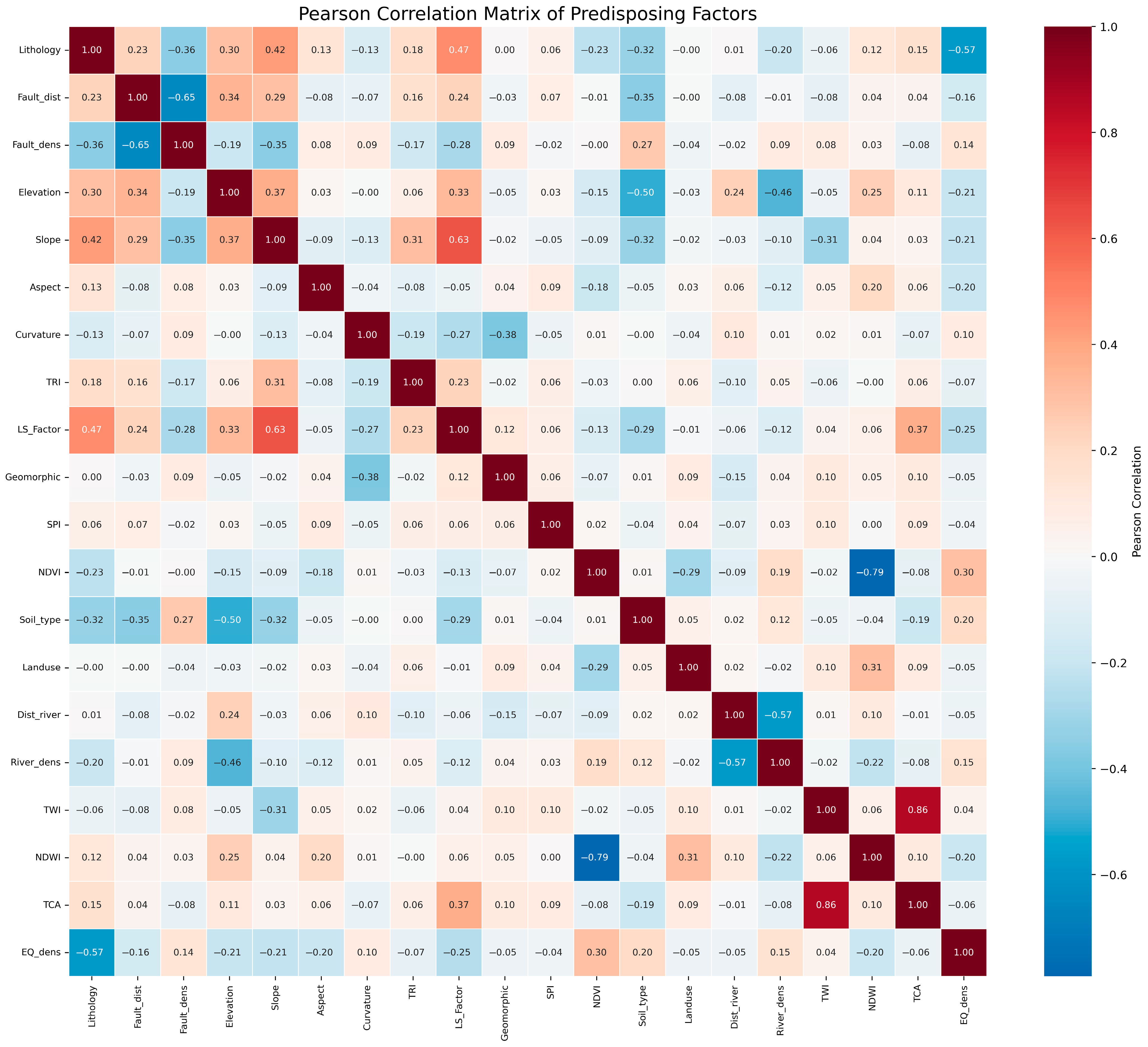
The redundancy assessment using Pearson correlation and VIF/TOL showed that most conditioning factors exhibited weak to moderate correlations, with values generally below |0.8|. However, a strong correlation was detected between TWI and TCA (r = 0.86), while the highest VIF values were observed for TCA (7.36), TWI (7.08), and NDWI (3.08). To reduce redundancy and improve model interpretability, TCA was excluded, resulting in a final set of 19 factors used for susceptibility modeling.

Following feature selection, all remaining factors were normalized using the Min–Max method to rescale values to the [0, 1] range, ensuring comparability across heterogeneous predictors. The dataset was then split into 80% sub-training and 20% validation sets, maintaining class balance between landslide and non-landslide samples. These preprocessing steps provided a consistent and reliable foundation for subsequent modeling. The outcomes of the correlation and multicollinearity analysis are summarized in Figure 8 and

Table 2. Multicollinearity assessment of input factors using VIF and TOL.

Factors	VIF	TOL	Factors	VIF	TOL
Lithology	2.13	0.47	SPI	1.06	0.95
Distance to fault	2.12	0.47	NDVI	3.03	0.33
Fault density	2.13	0.47	Soil type	1.58	0.63
Elevation	2.14	0.47	Landuse	1.16	0.86
Slope	2.51	0.40	Distance to the river	1.62	0.62
Aspect	1.15	0.87	River density	1.92	0.52
Curvature	1.32	0.76	TWI	7.08	0.14
TRI	1.21	0.83	NDWI	3.08	0.32
LS Factor	2.55	0.39	TCA	7.36	0.14
Geomorphic units	1.26	0.79	Earthquake density	1.62	0.62

, which confirm that the refined dataset is suitable for use in the subsequent modeling stage.

3.2. Modeling Results

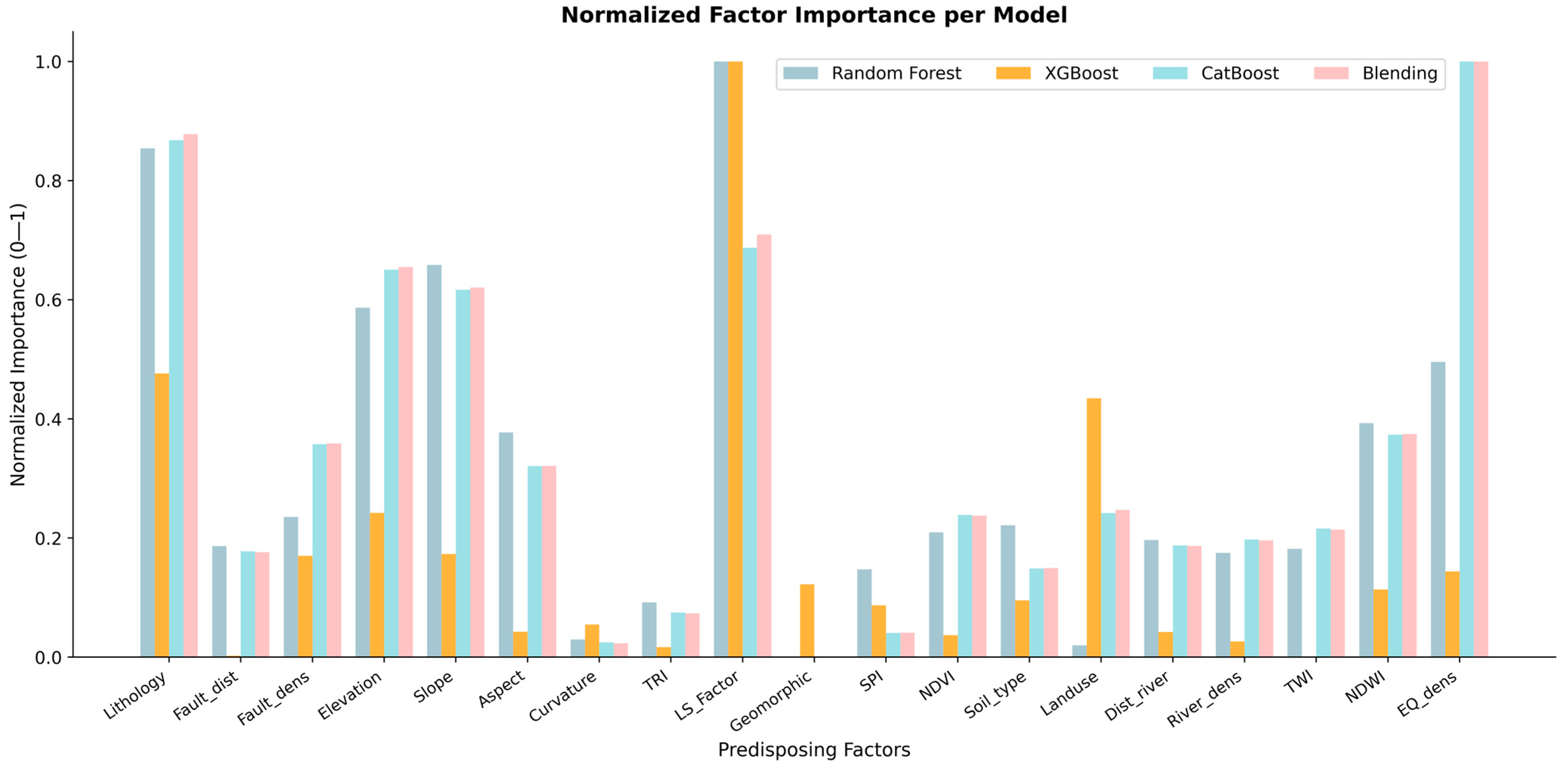
The modeling results highlighted the relative contributions of the conditioning factors as well as the spatial distribution of landslide susceptibility predicted by the four approaches: Random Forest, XGBoost, CatBoost, and the blended ensemble model. Factor importance analysis (Figure 9) indicated that lithology, LS Factor, and earthquake density consistently emerged as the most influential predictors across all models, with normalized importance values ranging between 0.15 and 1.00. Slope, elevation, and aspect also contributed significantly, particularly in the Random Forest and CatBoost models, with values typically between 0.30 and 0.80. In contrast, variables such as geomorphic units and curvature exhibited relatively minor influence, with normalized importance values below 0.10. Interestingly, XGBoost assigned a comparatively higher weight to land use (0.45) compared to the other algorithms, reflecting its sensitivity to localized anthropogenic drivers. The blended ensemble model integrated these complementary geological, geomorphological, and land-use controls on landslide occurrence.

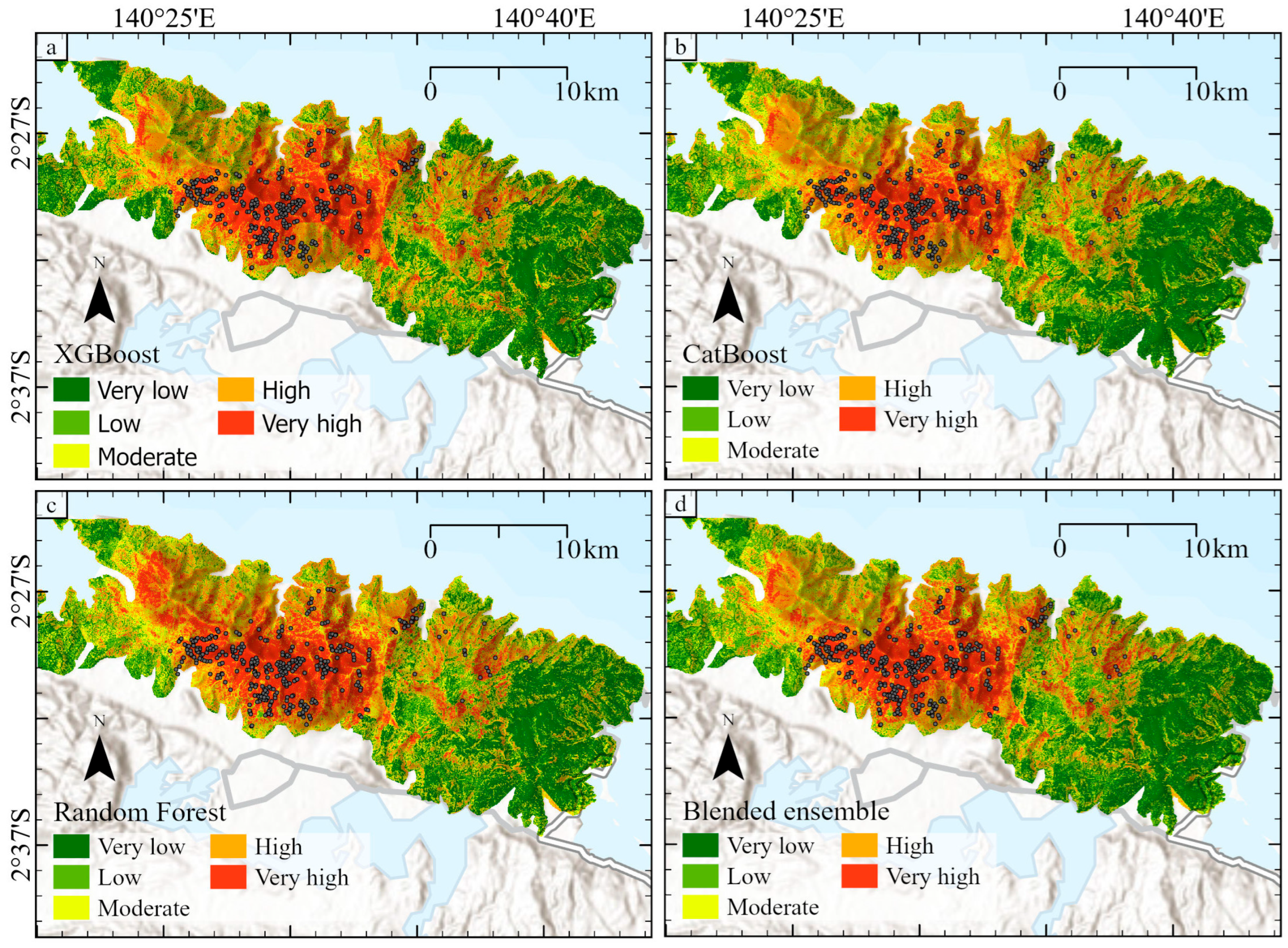
The susceptibility maps generated by each model (Figure 10) demonstrated broadly consistent spatial patterns, with high and very high susceptibility zones concentrated in the central and northern sectors of the study area, particularly along steep slopes and active fault zones. Nevertheless, model-specific differences were evident: the Random Forest and CatBoost maps delineated more continuous high-susceptibility belts, whereas XGBoost produced more fragmented patterns, especially in transitional slope zones. The blended ensemble map (Figure 10d) synthesized these perspectives, yielding a smoother and more balanced delineation of hazard-prone areas that corresponds well with the spatial distribution of observed landslides.

3.3. Validation and Interpretability Results

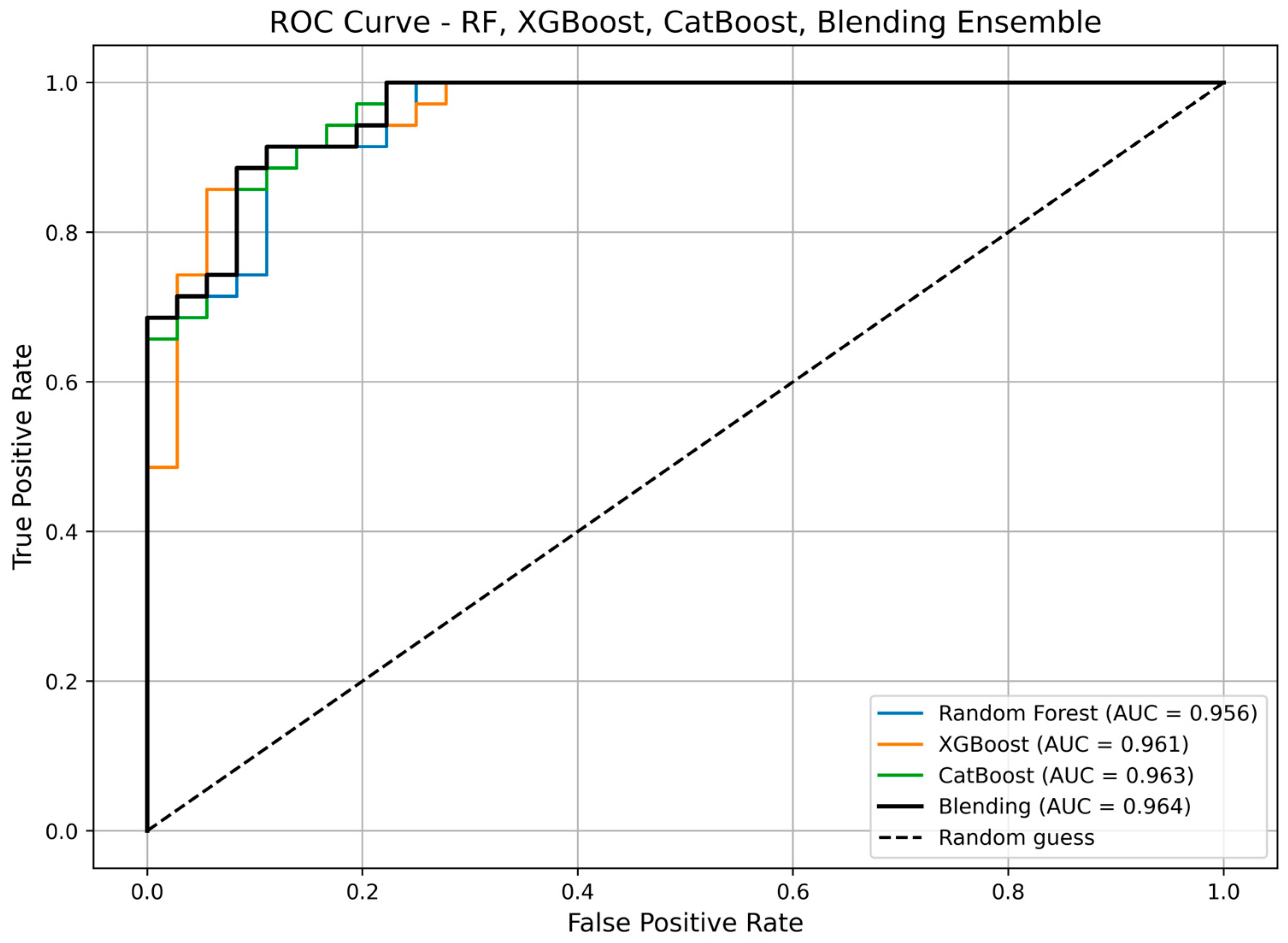
The four models—Random Forest, XGBoost, CatBoost, and the blended ensemble model—achieved consistently high predictive performance across all evaluation metrics (

Table 3. Summary results for the four models.

Model	AUC	Accuracy	Precision	Recall	F1-Score
Random Forest	0.956	0.887	0.886	0.886	0.886
XGBoost	0.961	0.887	0.886	0.886	0.886
CatBoost	0.963	0.887	0.886	0.886	0.886
Blending Ensemble	0.964	0.901	0.889	0.914	0.901

; Figure 11). AUC values ranged from 0.956 (Random Forest) to 0.964 (Blended Ensemble Model), all falling within the excellent category (>0.9). Accuracy scores were similarly high, ranging from 0.887 to 0.901, underscoring the reliability of the classifications. Precision values clustered between 0.886 and 0.889, indicating a low incidence of false positives, while recall values ranged from 0.886 to 0.914, reflecting strong sensitivity in detecting true landslide events. F1-scores mirrored these patterns, with the blended ensemble model achieving the highest balance (0.901). Among the individual learners, CatBoost slightly outperformed Random Forest and XGBoost, but the blended ensemble achieved the most consistent balance across all metrics. The ROC curves (Figure 11) further illustrated this stability, with all models approaching the upper-left corner and the blended ensemble model curve marginally dominating the others.

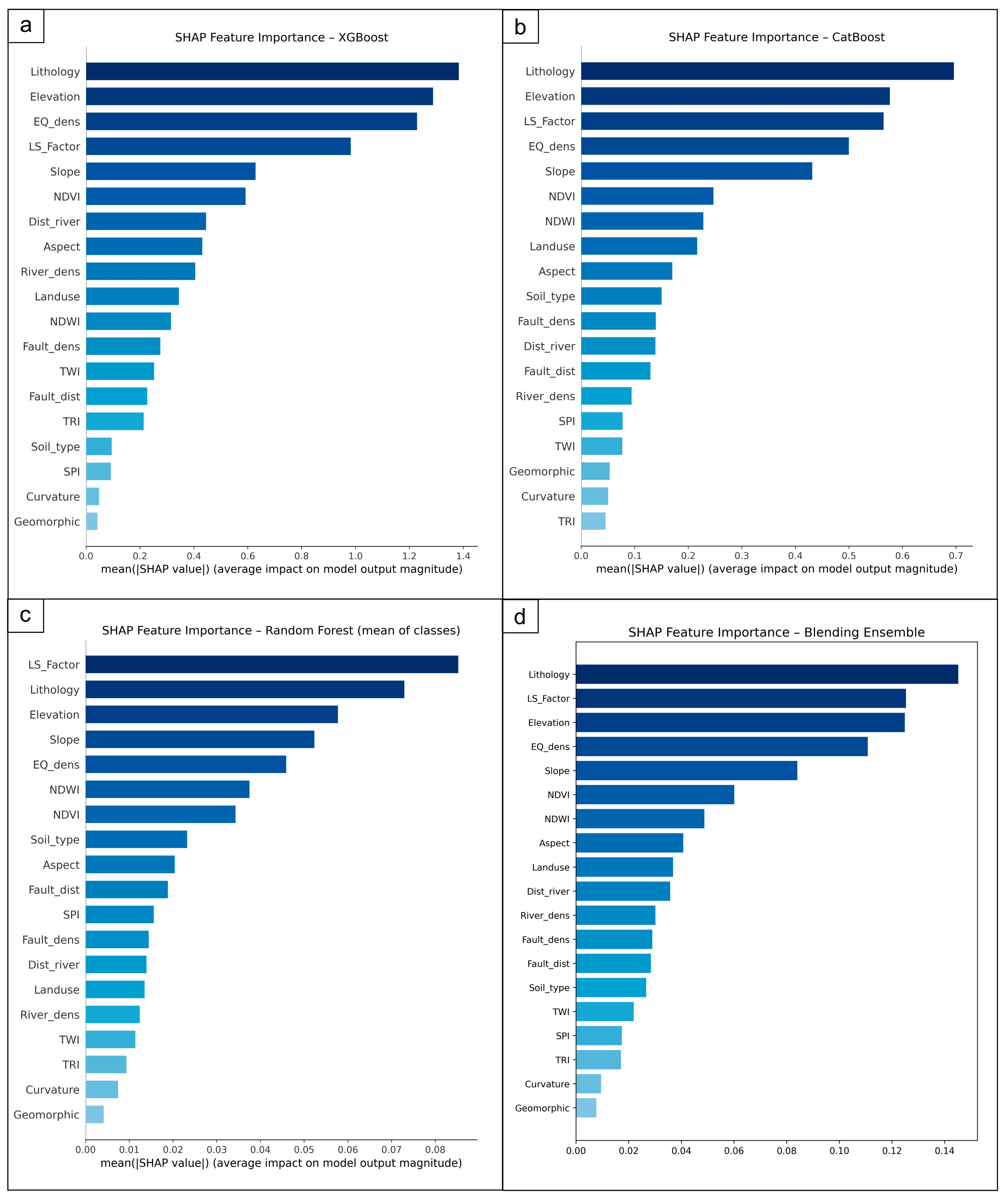
The interpretability analyses (Figure 12 and Figure 13) provide complementary insights into the relative weight of predictors and their directional influence on landslide susceptibility. The bar charts in Figure 12a–d show SHAP-based feature importance, which represents the mean absolute SHAP value of each predictor across all samples. Longer bars indicate stronger influence, with the highest-ranked features appearing at the top. Across the models, lithology and LS Factor consistently emerged as the most influential predictors, followed by slope, elevation, and earthquake density, while curvature and geomorphic units ranked among the least influential predictors. The blended ensemble model produced a more balanced ranking, which further reinforced lithology, LS Factor, and elevation as dominant predictors.

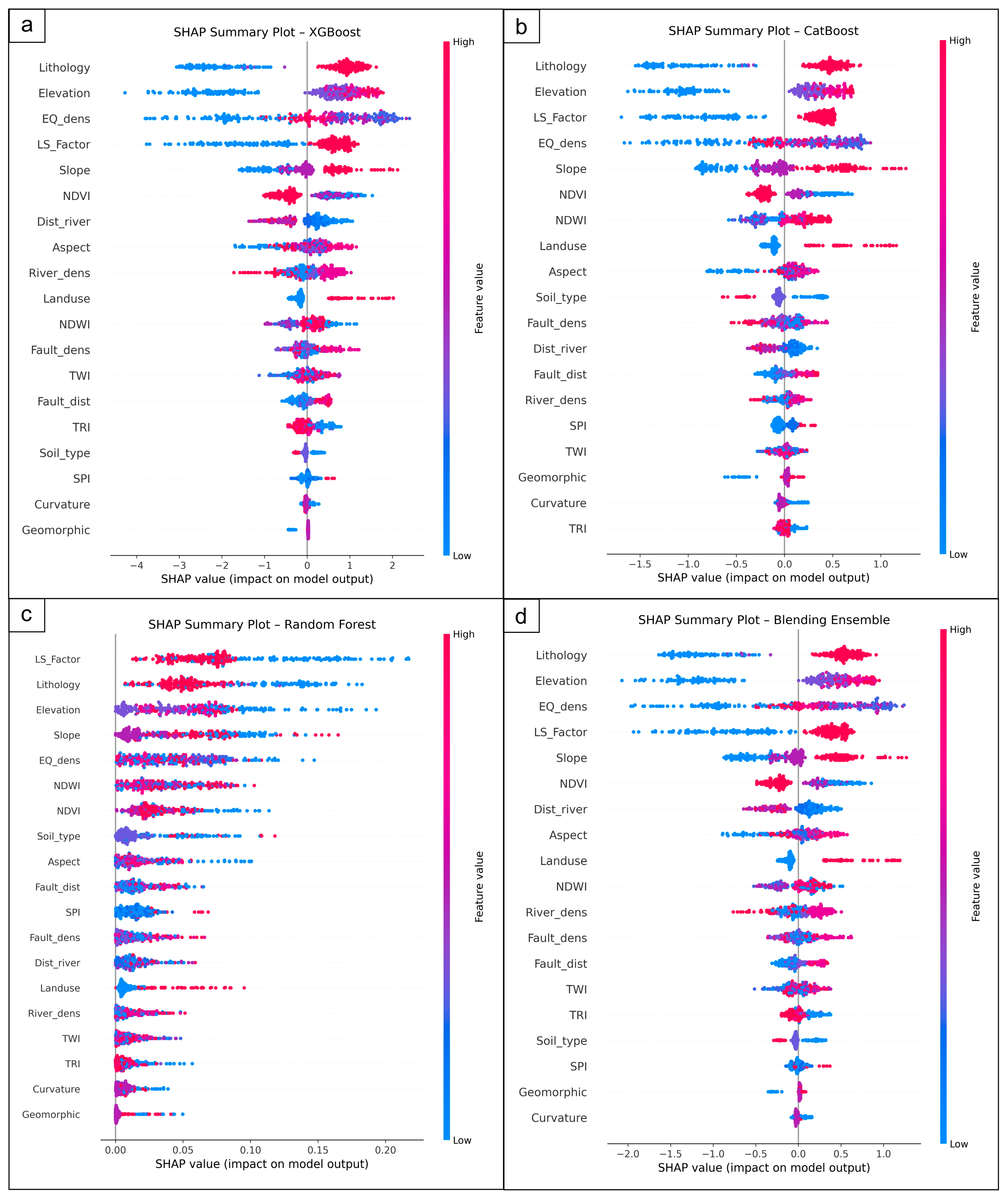
It is important to clarify that rankings derived from SHAP feature importance (Figure 12 and Figure 13) may differ from those obtained using normalized feature importance (Figure 9). This discrepancy does not indicate an error but reflects the methodological differences between the two approaches. Normalized feature importance measures how frequently or strongly a feature is used in the model’s structure, but it cannot show whether the feature increases or decreases susceptibility. In contrast, SHAP values provide a model-consistent and explainable metric, quantifying the actual marginal contribution of each predictor to the outcome (landslide susceptibility model). For Random Forest, SHAP captures average contributions across trees; for XGBoost and CatBoost it explains predictor effects within boosted ensembles; and for the blended ensemble SHAP reveals how base learners jointly transmit information into the meta-model.

The SHAP summary plots in Figure 13a–d further deepen interpretation by illustrating not only the magnitude but also the direction of influence. Each dot represents one observation, where the x-axis shows the SHAP value and the color encodes the feature value (red = high, blue = low). Across all models, LS Factor, lithology, and slope consistently dominated influence, with slope and LS Factor showing wide spreads that indicate strong context-dependent effects. The blending ensemble confirmed lithology, LS Factor, and elevation as the most decisive drivers, while NDVI contributed as a stabilizing factor by reducing susceptibility.

In the context of landslide susceptibility modeling, SHAP provides clear advantages over normalized feature importance. While normalized importance can indicate which factors the model relies on structurally, SHAP explicitly reveals how each environmental factor contributes to increasing or decreasing susceptibility. This level of explainability offers stronger and more reliable insights for understanding the physical drivers of landslides and supports more transparent hazard assessment and mitigation planning.

4. Discussion and Recommendations

The four machine learning approaches—Random Forest, XGBoost, CatBoost, and the blended ensemble model—achieved consistently high predictive accuracy, with AUC values exceeding 0.95. This placed them within the “excellent” category of classification models and confirmed their robustness for susceptibility mapping [60]. Although CatBoost slightly outperformed the other single learners, the blended ensemble achieved the most balanced performance across all evaluation metrics, with higher stability in detecting both true positives (recall) and reducing false alarms (precision). The ensemble’s marginal improvement reflected its ability to integrate the complementary strengths of individual models, resulting in a smoother and more reliable susceptibility assessment.

Across all models, lithology, LS Factor, slope, elevation, and earthquake density consistently emerged as dominant factors. Their prominence highlighted the combined influence of geological processes: weak lithological units and active tectonic settings created fundamental susceptibility, while steep slopes and concentrated runoff represented by the LS Factor further amplified hazard potential [63]. The sensitivity of XGBoost to land use also underscored the importance of anthropogenic modifications. In contrast, curvature and geomorphic units contributed little predictive power, suggesting that their role in this region was secondary relative to other conditioning factors.

The susceptibility maps produced by the different algorithms displayed broadly consistent spatial patterns, with high and very high susceptibility zones concentrated in steep slopes and in the fault-influenced northern and central sectors. However, subtle differences were evident. Random Forest and CatBoost produced more continuous high-susceptibility belts, whereas XGBoost depicted more fragmented distributions in transitional terrain. The blended ensemble map reconciled these differences, producing a balanced delineation that aligned closely with observed landslide occurrences. This spatial consistency across methods reinforced the reliability of the key predictors, while the differences highlighted the varying sensitivities of algorithms to terrain heterogeneity.

Validation confirmed the strong predictive performance of all models, with the blending ensemble achieving the most balanced results across evaluation metrics. Beyond accuracy, interpretability analyses added practical value. While normalized feature importance ranked predictors by their structural use in the models, SHAP provided deeper insights by quantifying whether high or low feature values increased or decreased susceptibility [64]. This distinction is crucial, as SHAP consistently highlighted lithology, LS Factor, and slope as dominant drivers, while NDVI emerged as a stabilizing factor that reduced susceptibility [65].

These findings suggest that areas characterized by vulnerable lithologies, steep slopes, and high LS Factor should be prioritized for monitoring and mitigation. At the same time, maintaining vegetation cover remains an effective strategy for reducing susceptibility. By combining ensemble learning with SHAP explainability, the study delivers not only robust predictive performance but also actionable guidance for hazard management and land-use planning.

5. Conclusions

This study applied an ensemble machine learning approach to landslide susceptibility mapping in the Sentani region of Papua, Indonesia, integrating geological, geomorphological, hydrological, environmental, and seismological datasets with a detailed landslide inventory. Methods used in this study included landslide susceptibility models using Random Forest, Boost, CatBoost, and a blended ensemble approach with 19 conditioning factors. All four models demonstrated excellent predictive capability, with AUC values exceeding 0.95, underscoring the reliability of machine learning for susceptibility assessment in complex mountainous terrain. The blended ensemble provided the most stable and balanced performance, integrating the strengths of individual learners.

Among the conditioning factors, lithology, LS Factor, slope, elevation, and earthquake density consistently emerged as the dominant drivers of landslide occurrence, reflecting the combined influence of geological weakness, topographic steepness, and tectonic activity. The role of land use was particularly pronounced in XGBoost, highlighting the local importance of anthropogenic modifications, whereas curvature and geomorphic units contributed little predictive value. The susceptibility maps revealed consistent spatial patterns across models, with high and very high susceptibility zones concentrated along steep slopes and active fault zones in the central and northern parts of the study area. These patterns closely correspond with observed landslide distributions, reinforcing the validity of the predictive framework.

Overall, the findings demonstrate that ensemble machine learning provides a powerful and interpretable tool for landslide susceptibility mapping. By integrating geological, geomorphological, and land-use factors, the approach not only captures the complexity of landslide processes but also delivers actionable outputs to inform hazard mitigation and land-use planning. For Sentani, where rapid settlement expansion intersects with vulnerable landscapes, the results provide a spatial basis to inform land-use planning, enhance preparedness, and reduce disaster risk. Future work should incorporate temporal dynamics, expanded inventories, and climate change scenarios to further strengthen regional resilience against landslides.

References

1. Jomelli, V.; Pavlova, I.; Giacona, F.; Zgheib, T.; Eckert, N. Respective Influence of Geomorphologic and Climate Conditions on Debris-Flow Occurrence in the Northern French Alps. Landslides 2019, 16, 1871–1883. [Google Scholar] [CrossRef]
2. Ballesteros-Cánovas, J.; Kariya, Y.; Imaizumi, F.; Manchado, A.; Nishii, R.; Matsuoka, N.; Stoffel, M. Debris-Flow Activity in the Japanese Alps Is Controlled by Extreme Precipitation and ENSO—Evidence from Multi-Centennial Tree-Ring Records. Glob. Planet. Change 2023, 231, 104296. [Google Scholar] [CrossRef]
3. Guzzetti, F.; Peruccacci, S.; Rossi, M.; Stark, C.P. The Rainfall Intensity–Duration Control of Shallow Landslides and Debris Flows: An Update. Landslides 2008, 5, 3–17. [Google Scholar] [CrossRef]
4. Baum, R.L.; Godt, J.W. Early Warning of Rainfall-Induced Shallow Landslides and Debris Flows in the USA. Landslides 2010, 7, 259–272. [Google Scholar] [CrossRef]
5. Jakob, M.; Hungr, O. Debris-Flow Hazards and Related Phenomena, 1st ed.; Springer: Berlin/Heidelberg, Germany, 2005. [Google Scholar]
6. Ishizuka, T.; Kaji, A.; Morita, K.; Mori, T.; Chiba, M.; Kashiwabara, Y.; Yoshino, K.; Uchida, T.; Mizuyama, T. Analysis for a Landslide Dam Outburst Flood in Ambon Island, Indonesia. Int. J. Eros. Control Eng. 2017, 10, 32–38. [Google Scholar] [CrossRef]
7. Larsen, M.C.; Wieczorek, G.F.; Eaton, L.S.; Morgan, B.A.; Torres-Sierra, H. Venezuelan Debris Flow and Flash Flood Disaster of 1999 Studied. Eos Trans. Am. Geophys. Union 2001, 82, 572–573. [Google Scholar] [CrossRef]
8. Rodolfo, K.S.; Lagmay, A.M.F.; Eco, R.C.; Herrero, T.M.L.; Mendoza, J.E.; Minimo, L.G.; Santiago, J.T. The December 2012 Mayo River Debris Flow Triggered by Super Typhoon Bopha in Mindanao, Philippines: Lessons Learned and Questions Raised. Nat. Hazards Earth Syst. Sci. 2016, 16, 2683–2695. [Google Scholar] [CrossRef]
9. Froude, M.J.; Petley, D.N. Global Fatal Landslide Occurrence from 2004 to 2016. Nat. Hazards Earth Syst. Sci. 2018, 18, 2161–2181. [Google Scholar] [CrossRef]
10. Kompas Banjir Bandang Sentani, Tiga Tahun Berselang. Available online: https://www.kompas.id/artikel/banjir-bandang-sentani-tiga-tahun-berselang (accessed on 31 August 2025).
11. Kristiawan, Y.; Budianto, A.; Santosa, I.; Suryadana, K.M. Untuk Tanggap Darurat Banjir Bandang Sentani, Debris Flow Modelling for Emergency Response on Debris. 2021. Available online: https://www.researchgate.net/publication/350310308 (accessed on 1 September 2025).
12. Arango-carmona, M.I.; Voit, P.; Hürlimann, M.; Aristizábal, E.; Korup, O. Hillslope-Torrential Hazard Cascades in Tropical Mountains. EGUsphere 2025, 2025, 1–30. [Google Scholar] [CrossRef]
13. Fell, R.; Corominas, J.; Bonnard, C.; Cascini, L.; Leroi, E.; Savage, W.Z. Guidelines for Landslide Susceptibility, Hazard and Risk Zoning for Land-Use Planning. Eng. Geol. 2008, 102, 99–111. [Google Scholar] [CrossRef]
14. Cascini, L. Applicability of Landslide Susceptibility and Hazard Zoning at Different Scales. Eng. Geol. 2008, 102, 164–177. [Google Scholar] [CrossRef]
15. Casagli, N.; Frodella, W.; Morelli, S.; Tofani, V.; Ciampalini, A.; Intrieri, E.; Raspini, F.; Rossi, G.; Tanteri, L.; Lu, P. Spaceborne, UAV and Ground-Based Remote Sensing Techniques for Landslide Mapping, Monitoring and Early Warning. Geoenvironmental Disasters 2017, 4, 9. [Google Scholar] [CrossRef]
16. Breiman, L. Random Forests. Mach. Learn. 2001, 45, 5–32. [Google Scholar] [CrossRef]
17. Chen, T.; Guestrin, C. XGBoost: A Scalable Tree Boosting System. In Proceedings of the 22nd ACM SIGKDD International Conference on Knowledge Discovery and Data Mining, San Francisco, CA, USA, 13–17 August 2018; pp. 785–794. [Google Scholar] [CrossRef]
18. Prokhorenkova, L.; Gusev, G.; Vorobev, A.; Dorogush, A.V.; Gulin, A. Catboost: Unbiased Boosting with Categorical Features. Adv. Neural Inf. Process. Syst. 2018, 31, 6638–6648. [Google Scholar]
19. Ganaie, M.A.; Hu, M.; Malik, A.K.; Tanveer, M.; Suganthan, P.N. Ensemble Deep Learning: A Review. Eng. Appl. Artif. Intell. 2022, 115, 105151. [Google Scholar] [CrossRef]
20. Mienye, I.D.; Sun, Y. A Survey of Ensemble Learning: Concepts, Algorithms, Applications, and Prospects. IEEE Access 2022, 10, 99129–99149. [Google Scholar] [CrossRef]
21. European Space Agency (ESA) Copernicus Browser. Copernicus Data Space Ecosystem. Available online: https://dataspace.copernicus.eu/ (accessed on 1 September 2025).
22. VOA Indonesia BNPB: Banjir Bandang Sentani Akibat Ulah Manusia Yang Merusak Alam. Available online: https://www.voaindonesia.com/a/bnpb-banjir-bandang-sentani-akibat-ulah-manusia-yang-merusak-alam/4836093.html (accessed on 1 September 2025).
23. BBC Indonesia Banjir Sentani, Papua: Curah Hujan Masih Tinggi, Waspadai Banjir Susulan. Available online: https://www.bbc.com/indonesia/indonesia-47600617 (accessed on 1 September 2025).
24. Diamond, J.; Bishop, K.D. Why Are New Guinea’s Cyclops Mountains Poor in Upland Bird Species? Bull. Br. Ornithol. Club 2025, 145, 60–90. [Google Scholar] [CrossRef]
25. BRIN Attenborough’s Long-Beaked Echidna Rediscovered in Papua. Available online: https://www.brin.go.id/en/news/116646/attenboroughs-long-beaked-echidna-rediscovered-in-papua (accessed on 2 September 2025).
26. Suwarna, N.; Noya, Y. Geological Map of The Jayapura (Peg. Cyclops) Quadrangle, Irian Jaya Scale 1:250.000 1995. Available online: https://geologi.esdm.go.id/geomap/pages/preview/peta-geologi-lembar-gunung-doom-irian-jaya (accessed on 2 September 2025).
27. IRIS Interactive Earthquake Browser—Global Earthquake Catalog. Available online: https://ds.iris.edu/ (accessed on 1 March 2025).
28. BMKG Earthquake Event Catalog. Jakarta: BMKG. Available online: https://repogempa.bmkg.go.id/eventcatalog (accessed on 1 March 2025).
29. BIG Ina-Geoportal Geospasial Untuk Negeri. Available online: https://tanahair.indonesia.go.id/portal-web/ (accessed on 1 May 2025).
30. Hengl, T.; Mendes de Jesus, J.; Heuvelink, G.B.M.; Ruiperez Gonzalez, M.; Kilibarda, M.; Blagotić, A.; Shangguan, W.; Wright, M.N.; Geng, X.; Bauer-Marschallinger, B.; et al. SoilGrids250m: Global Gridded Soil Information Based on Machine Learning. PLoS ONE 2017, 12, e0169748. [Google Scholar] [CrossRef]
31. Zanaga, D.; Van De Kerchove, R.; Daems, D.; De Keersmaecker, W.; Brockmann, C.; Kirches, G.; Wevers, J.; Cartus, O.; Santoro, M.; Fritz, S.; et al. ESA WorldCover 10 m 2021 V200 2022. 2022. Available online: https://research.wur.nl/en/datasets/esa-worldcover-10-m-2021-v200 (accessed on 1 September 2025). [CrossRef]
32. Lee, S.; Talib, J.A. Probabilistic Landslide Susceptibility and Factor Effect Analysis. Environ. Geol. 2005, 47, 982–990. [Google Scholar] [CrossRef]
33. Kamp, U.; Growley, B.J.; Khattak, G.A.; Owen, L.A. GIS-Based Landslide Susceptibility Mapping for the 2005 Kashmir Earthquake Region. Geomorphology 2008, 101, 631–642. [Google Scholar] [CrossRef]
34. Price, K. Effects of Watershed Topography, Soils, Land Use, and Climate on Baseflow Hydrology in Humid Regions: A Review. Prog. Phys. Geogr. 2011, 35, 465–492. [Google Scholar] [CrossRef]
35. Fusco, F.; De Vita, P.; Mirus, B.B.; Baum, R.L.; Allocca, V.; Tufano, R.; Di Clemente, E.; Calcaterra, D. Physically Based Estimation of Rainfall Thresholds Triggering Shallow Landslides in Volcanic Slopes of Southern Italy. Water 2019, 11, 1915. [Google Scholar] [CrossRef]
36. Çellek, S. The Effect of Aspect on Landslide and Its Relationship with Other Parameters; Zhang, Y., Cheng, Q., Eds.; IntechOpen: Rijeka, Croatia, 2021; ISBN 978-1-83969-024-2. [Google Scholar]
37. Nakileza, B.R.; Nedala, S. Topographic Influence on Landslides Characteristics and Implication for Risk Management in Upper Manafwa Catchment, Mt Elgon Uganda. Geoenvironmental Disasters 2020, 7, 27. [Google Scholar] [CrossRef]
38. Rózycka, M.; Migoń, P.; Michniewicz, A. Topographic Wetness Index and Terrain Ruggedness Index in Geomorphic Characterisation of Landslide Terrains, on Examples from the Sudetes, SW Poland. Z. Fur Geomorphol. 2017, 61, 61–80. [Google Scholar] [CrossRef]
39. Zhang, H.; Wei, J.; Yang, Q.; Baartman, J.E.M.; Gai, L.; Yang, X.; Li, S.Q.; Yu, J.; Ritsema, C.J.; Geissen, V. An Improved Method for Calculating Slope Length (λ) and the LS Parameters of the Revised Universal Soil Loss Equation for Large Watersheds. Geoderma 2017, 308, 36–45. [Google Scholar] [CrossRef]
40. Muddarisna, N.; Yuniwati, E.D.; Masruroh, H.; Oktaviansyah, A.R. An Automated Approach Using Topographic Position Index (TPI) for Landform Mapping (Case Study: Gede Watershed, Malang Regency, East Java, Indonesia). IOP Conf. Ser. Earth Environ. Sci. 2020, 412. [Google Scholar] [CrossRef]
41. Chen, C.Y.; Chang, J.M. Landslide Dam Formation Susceptibility Analysis Based on Geomorphic Features. Landslides 2016, 13, 1019–1033. [Google Scholar] [CrossRef]
42. Dahigamuwa, T.; Yu, Q.; Gunaratne, M. Feasibility Study of Land Cover Classification Based on Normalized Difference Vegetation Index for Landslide Risk Assessment. Geosciences 2016, 6, 45. [Google Scholar] [CrossRef]
43. Bhagya, S.B.; Sumi, A.S.; Balaji, S.; Danumah, J.H.; Costache, R.; Rajaneesh, A.; Gokul, A.; Chandrasenan, C.P.; Quevedo, R.P.; Johny, A.; et al. Landslide Susceptibility Assessment of a Part of the Western Ghats (India) Employing the AHP and F-AHP Models and Comparison with Existing Susceptibility Maps. Land 2023, 12, 468. [Google Scholar] [CrossRef]
44. Formetta, G.; Capparelli, G.; Versace, P. Evaluating Performance of Simplified Physically Based Models for Shallow Landslide Susceptibility. Hydrol. Earth Syst. Sci. 2016, 20, 4585–4603. [Google Scholar] [CrossRef]
45. Hong, H.; Shahabi, H.; Shirzadi, A.; Chen, W.; Chapi, K.; Ahmad, B.B.; Roodposhti, M.S.; Yari Hesar, A.; Tian, Y.; Tien Bui, D. Landslide Susceptibility Assessment at the Wuning Area, China: A Comparison between Multi-Criteria Decision Making, Bivariate Statistical and Machine Learning Methods. Nat. Hazards 2019, 96, 173–212. [Google Scholar] [CrossRef]
46. Wang, Y.; Fang, Z.; Hong, H. Comparison of Convolutional Neural Networks for Landslide Susceptibility Mapping in Yanshan County, China. Sci. Total Environ. 2019, 666, 975–993. [Google Scholar] [CrossRef] [PubMed]
47. Goetz, J.N.; Brenning, A.; Petschko, H.; Leopold, P. Evaluating Machine Learning and Statistical Prediction Techniques for Landslide Susceptibility Modeling. Comput. Geosci. 2015, 81, 1–11. [Google Scholar] [CrossRef]
48. Hong, H.; Pradhan, B.; Sameen, M.I.; Kalantar, B.; Zhu, A.; Chen, W. Improving the Accuracy of Landslide Susceptibility Model Using a Novel Region-Partitioning Approach. Landslides 2018, 15, 753–772. [Google Scholar] [CrossRef]
49. Pham, B.T.; Tien Bui, D.; Prakash, I. Bagging Based Support Vector Machines for Spatial Prediction of Landslides. Environ. Earth Sci. 2018, 77, 146. [Google Scholar] [CrossRef]
50. Kritikos, T.; Davies, T. Assessment of Rainfall-Generated Shallow Landslide/Debris-Flow Susceptibility and Runout Using a GIS-Based Approach: Application to Western Southern Alps of New Zealand. Landslides 2015, 12, 1051–1075. [Google Scholar] [CrossRef]
51. Chen, W.; Xie, X.; Peng, J.; Shahabi, H.; Hong, H.; Bui, D.T.; Duan, Z.; Li, S.; Zhu, A.-X. GIS-Based Landslide Susceptibility Evaluation Using a Novel Hybrid Integration Approach of Bivariate Statistical Based Random Forest Method. Catena (Amst) 2018, 164, 135–149. [Google Scholar] [CrossRef]
52. Liu, D.; Xiang, Q.; Sang, X.; Zhang, S.; Yang, H. Landslide Susceptibility Prediction Method Based on HSOM and IABPA-CNN in Wenchuan Earthquake Disaster Area. J. Mt. Sci. 2024, 21, 4001–4018. [Google Scholar] [CrossRef]
53. Lee, S.-M.; Lee, S.-J. Landslide Susceptibility Assessment of South Korea Using Stacking Ensemble Machine Learning. Geoenvironmental Disasters 2024, 11, 7. [Google Scholar] [CrossRef]
54. Tong, T.; Li, Z. Predicting Learning Achievement Using Ensemble Learning with Result Explanation. PLoS ONE 2025, 20, e0312124. [Google Scholar] [CrossRef]
55. Wolpert, D.H. Stacked Generalization. Neural Netw. 1992, 5, 241–259. [Google Scholar] [CrossRef]
56. Zhou, Z.-H. Ensemble Methods: Foundations and Algorithms, 1st ed.; Chapman and Hall/CRC: Boca Raton, FL, USA, 2012. [Google Scholar]
57. Biau, G.; Scornet, E. A Random Forest Guided Tour. TEST 2016, 25, 197–227. [Google Scholar] [CrossRef]
58. Bishop, C.M. Pattern Recognition and Machine Learning; Springer: Berlin/Heidelberg, Germany, 2006. [Google Scholar]
59. Hastie, T.; Tibshirani, R.; Friedman, J. The Elements of Statistical Learning: Data Mining, Inference, and Prediction, 2nd ed.; Springer: Berlin/Heidelberg, Germany, 2009. [Google Scholar]
60. Pham, B.T.; Pradhan, B.; Tien Bui, D.; Prakash, I.; Dholakia, M.B. A Comparative Study of Different Machine Learning Methods for Landslide Susceptibility Assessment. Environ. Model. Softw. 2016, 84, 240–250. [Google Scholar] [CrossRef]
61. Lundberg, S.M.; Erion, G.; Chen, H.; DeGrave, A.; Prutkin, J.M.; Nair, B.; Katz, R.; Himmelfarb, J.; Bansal, N.; Lee, S.-I. From Local Explanations to Global Understanding with Explainable AI for Trees. Nat. Mach. Intell. 2020, 2, 56–67. [Google Scholar] [CrossRef]
62. Lundberg, S.M.; Lee, S.-I. A Unified Approach to Interpreting Model Predictions. Adv. Neural Inf. Process. Syst. 2017, 30, 4765–4774. [Google Scholar]
63. Merghadi, A.; Yunus, A.P.; Dou, J.; Whiteley, J.; ThaiPham, B.; Bui, D.T.; Avtar, R.; Abderrahmane, B. Machine Learning Methods for Landslide Susceptibility Studies: A Comparative Overview of Algorithm Performance. Earth Sci. Rev. 2020, 207, 103225. [Google Scholar] [CrossRef]
64. Sun, D.; Ding, Y.; Wen, H.; Zhang, F.; Zhang, J.; Gu, Q.; Zhang, J. SHAP-PDP Hybrid Interpretation of Decision-Making Mechanism of Machine Learning-Based Landslide Susceptibility Mapping: A Case Study at Wushan District, China. Egypt. J. Remote Sens. Space Sci. 2024, 27, 508–523. [Google Scholar] [CrossRef]
65. Usta, Z.; Akıncı, H.; Akın, A.T. Comparison of Tree-Based Ensemble Learning Algorithms for Landslide Susceptibility Mapping in Murgul (Artvin), Turkey. Earth Sci. Inf. 2024, 17, 1459–1481. [Google Scholar] [CrossRef]
Figure 2. (a). Geological setting of the Cyclops Mountains, showing the dominance of metamorphic (pTmc) and ultramafic rocks (um) (b). Seismicity distribution in the region, including Mw 5.5 earthquakes recorded in Doyo Baru (2015) and Jayapura (2023).
Geosciences 15 00390 g002
Figure 3. Temporal distribution of seismic events, emphasizing the 2022–2023 sequence showing increased tectonic activity and hazard potential in the region.
Geosciences 15 00390 g003
Figure 4. (a) Spatial distribution of mapped landslides in the Cyclops Mountains from 2015 to 2025 with red polygons represent detected landslides. (a.1d.1) Pre-event imagery (5 February 2019) and (a.2d.2) post-event imagery (25 June 2019) of the evaluation area using (a.1,a.2) true color composites, (b.1,b.2) Moisture Index, (c.1,c.2) false color composites, and (d.1,d.2) NDVI layers. Yellow outlines indicate mapped landslide boundaries.
Geosciences 15 00390 g004
Figure 5. Conditioning factors used for landslide susceptibility modeling in the Sentani area: (1) lithology; (2) distance to fault; (3) fault density; (4) elevation; (5) slope; (6) aspect; (7) curvature; (8) TRI; (9) LS factor; (10) geomorphic unit; (11) SPI; (12) NDVI; (13) soil type; (14) land use; (15) distance to river; (16) river density; (17) TWI; (18) NDWI; (19) TCA; and (20) earthquake density; (21) Spatial distribution of landslide (black) and non-landslide (red) sample points used in the susceptibility model, overlaid on the elevation background.
Geosciences 15 00390 g005
Figure 6. Workflow of the landslide susceptibility modeling using a blended ensemble model (RF, XGBoost, CatBoost, and Logistic Regression). The workflow consists of five stages: data input, preprocessing, modeling, validation, and susceptibility mapping/zonation.
Geosciences 15 00390 g006
Figure 7. Blended ensemble modeling workflow. The input dataset is first processed by three base learners (Random Forest, XGBoost, and CatBoost). Their probabilistic outputs are then combined by a Logistic Regression meta-learner to generate the final blended ensemble prediction model.
Geosciences 15 00390 g007
Figure 8. Pearson correlation matrix of the 20 landslide predisposing factors. Strong correlations appear among several hydrological variables, notably TWI and TCA.
Geosciences 15 00390 g008
Figure 9. Normalized importance scores (0–1) of landslide predisposing factors as computed by Random Forest, XGBoost, CatBoost, and the blended ensemble model.
Geosciences 15 00390 g009
Figure 10. Landslide susceptibility maps from (a) XGBoost, (b) CatBoost, (c) Random Forest, and (d) Blended Ensemble Model. Susceptibility is classified into five levels from very low to very high. Black dots show past landslides. The area is divided into nine blocks: West, Center–East (horizontal), and North–Center–South (vertical) for discussion.
Geosciences 15 00390 g010
Figure 11. Receiver Operating Characteristic (ROC) curves for Random Forest, XGBoost, CatBoost, and the blended ensemble model, with corresponding AUC scores.
Geosciences 15 00390 g011
Figure 12. SHAP-based model explainability across (a) XGBoost, (b) CatBoost, (c) Random Forest, and (d) Blending Ensemble. Bar plots of mean SHAP feature importance.
Geosciences 15 00390 g012
Figure 13. SHAP-based model explainability across (a) XGBoost, (b) CatBoost, (c) Random Forest, and (d) Blending Ensemble. SHAP summary plots showing value distribution and impact direction.
Geosciences 15 00390 g013