Abstract
Accurate inversion of the T2 spectrum of shale oil reservoir fluids is crucial for reservoir evaluation. However, traditional nuclear magnetic resonance inversion methods face challenges in extracting features from multi-exponential decay signals. This study proposed an inversion method that combines autoencoder (AE) and Fourier transform, aiming to enhance the accuracy and stability of T2 spectrum estimation for shale oil reservoirs. The autoencoder is employed to automatically extract deep features from the echo train, while the Fourier transform is used to enhance frequency domain features of multi-exponential decay information. Furthermore, this paper designs a customized weighted loss function based on a self-attention mechanism to focus the model’s learning capability on peak regions, thereby mitigating the negative impact of zero-value regions on model training. Experimental results demonstrate significant improvements in inversion accuracy, noise resistance, and computational efficiency compared to traditional inversion methods. This research provides an efficient and reliable new approach for precise evaluation of the T2 spectrum in shale oil reservoirs.
1. Introduction
The development and evaluation of shale oil reservoirs are crucial for the effective utilization of oil and gas resources, with the precise characterization of reservoir fluid properties being a core task in reservoir evaluation. Nuclear magnetic resonance (NMR) technology has been widely applied in the evaluation of unconventional oil and gas reservoirs due to its ability to non-destructively measure the pore structure and distribution characteristics of fluids. However, the complex pore structures and diverse fluid types in shale oil reservoirs result in NMR signals exhibiting multi-exponential decay characteristics [1]. Traditional T2 spectrum inversion methods often face issues of insufficient accuracy and sensitivity to noise when addressing this complexity.
NMR inversion essentially involves solving the first kind of Fredholm integral equation. Such ill-posed problems can cause significant fluctuations in the inversion spectrum due to minor noise in the original signal. Since Prammer (1994) introduced the use of truncated singular value decomposition (TSVD) for NMR logging inversion, TSVD has seen broad adoption in NMR T2-spectrum inversion and has spawned numerous refinements [2,3]. Ge Xinmin et al. (2016) integrated truncated singular value decomposition (TSVD) with particle swarm optimization (PSO), employing TSVD as a warm start for PSO to reduce iterations and improve inversion efficiency—an exemplar of hybrid algorithms that marry TSVD with metaheuristic optimizers [4]. Weng Aihua et al. (2002) proposed a new NMR inversion algorithm based on regression M-estimation methods, considering that NMR logging errors do not follow a normal distribution [5]. Jiang Ruizhong et al. (2005) improved the SVD algorithm by introducing non-negativity constraints to enhance result continuity in response to discontinuities in spectral peaks [6].
For low-SNR logging data, systematic comparisons showed that regularized inversion can outperform improved SVD when SNR is below ~30, whereas at higher SNR the opposite may hold, highlighting the importance of noise regime in method selection [7]. Beyond time-domain processing, Venkataramanan et al. established Mellin-transform methods that compute moments of T2 directly from CPMG data and offer robustness in inhomogeneous fields, providing an alternative to direct inverse-Laplace reconstructions [8,9].
To improve resolution or reduce sensitivity to hyper-parameter tuning, researchers explored hybrid or stochastic optimization schemes. For example, Ge et al. combined iterative TSVD with a parallel particle swarm optimization (PSO) to jointly invert relaxation spectra (extensible to 2D cases), which reduced iteration counts and improved stability on difficult datasets [10]. Monte-Carlo optimization/annealing has also been used to sample families of admissible spectra and report statistically smoothed inversions, offering robustness to multimodality and local minima [11]. In addition, Backus–Gilbert (BG) theory has been introduced to NMR relaxation inversion to explicitly control resolution versus variance, enabling stable reconstructions under strong noise [12].
With the rise of data-driven approaches, artificial neural networks (ANNs) have been applied to invert relaxation distributions directly from echo trains. Parasram and co-authors trained fully connected networks to recover both discrete and continuous T2 spectra, reporting higher accuracy than classical ILT baselines under suitable SNRs and training coverage [13]. Luo et al. further designed an autoencoder-style model (with attention/convolutional components) tailored for multi-exponential inversion and demonstrated accurate recovery across noisy settings, underscoring the value of feature engineering and network design for NMR relaxometry [14]. These works are in line with broader analyses arguing that multivariate learning and ANNs can complement Fourier/Laplace-like processing in low-field NMR by extracting latent structure from noisy exponential decays [15].
Inverse-Laplace recovery of the one-dimensional T2 spectrum from CPMG echoes is a classic ill-posed problem: traditional algorithms (e.g., TSVD/NNLS with regularization) are sensitive to noise and often under-resolve narrow peaks, especially in shale-oil settings where signals are weak and spectra are sparse. Recent work therefore turns to deep learning to exploit richer representations of the echo train and to alleviate the instability of purely model-based inversions.
In this study we combine an autoencoder (AE) with Fourier-derived features to enhance the accuracy and stability of T2 spectrum inversion for shale-oil reservoirs. The AE automatically extracts deep representations from the echoes, while the Fourier transform supplies complementary magnitude and phase information that highlights the multi-exponential decay characteristics in the frequency domain. To prevent long zero-valued bins from dominating the objective and to focus learning on informative peaks, we adopt a sparsity-aware weighted loss (rather than plain MSE). This weighting is not a transformer-style self-attention module; it is a deterministic, data-dependent reweighting designed to improve peak fidelity in T2 inversion.
Our goal is an efficient, robust deep model for shale-oil T2 spectrum inversion and an experimental validation of its benefits in inversion accuracy, noise robustness, and computational efficiency. The main contributions are:
- (i)
- a time-frequency hybrid input that concatenates the raw echo train with its Fourier magnitude and phase spectra, enabling multi-scale feature extraction;
- (ii)
- a sparsity-aware weighted loss that emphasizes peak regions while controlling the influence of extensive zero bins;
- (iii)
- a shale-oil-anchored evaluation, where synthetic datasets are guided by core-observed T2 peak ranges and tested over realistic SNR regimes.
Together, these elements yield markedly improved reconstructions of multi-peak T2 spectra and provide a practical pipeline for shale-oil reservoir characterization, while laying a solid foundation for subsequent extensions to 2D spectra.
2. Theoretical Basis of NMR Spectrum Inversion
Reservoir rocks typically exhibit a distribution of pore sizes and often contain multiphase fluids such as water, oil, and gas. Consequently, the CPMG pulse sequence records a spin-echo train that represents a distribution of transverse relaxation times T2, which can be expressed as:
where
- —measured magnetization at time ;
- —initial magnetization associated with the -th pore;
- —transverse relaxation time of the i-th pore (in seconds).
In the above expression, is proportional to the volume of the pore fluid, and the bulk signal amplitude detected from the formation at = 0, , equals the sum of the contributions from all pores:
If the measured initial magnetization for 100% free water within the same sensitive volume is known and denoted , then can be calibrated to porosity:
where
- —calibrated porosity of the formation (%);
- —calibrated porosity associated with the i-th pore (%).
In practice, treating each individual pore separately is intractable. Pores with similar surface-to-volume ratios—and hence fluids with similar T2 values—are grouped together. Under this grouping, the summation in the magnetization expression has a finite number of terms. Specifically, the T2 axis is partitioned into a finite set of intervals, and the T2 distribution is discretized into N distinct relaxation times (the “grid points”). The index i then refers to T2 bins rather than individual pores. If M points are sampled from the original echo train (typically M ≫ N), the M echo amplitudes and the N transverse-relaxation components form an M × N forward system:
where
- —acquisition time of the m-th echo (s), with = mTE;
- —porosity fraction corresponding to the n-th T2 time T2, n (%).
The above can be written in matrix form:
where
- S—vector of M echo amplitudes (M × 1);
- K—decay-coefficient (kernel) matrix for the N transverse-relaxation components across M echoes (M × N);
- f—vector of porosity fractions for the N T2 bins (N × 1, in %).
Through the foregoing system of equations, one can clearly understand the bulk T2 distribution model of a porous medium and forward-simulate it into the experimentally measured relaxation-echo signal. Specifically, the relaxation behavior of an individual pore is first characterized by its relaxation equation; the contributions from different pores are then superposed in a weighted manner to yield the overall T2 spectrum. Using this T2 spectrum in the matrix-form forward model of the NMR signal, the macroscopic, observable NMR echo train can be computed. This bottom-up modeling approach provides a complete and transparent theoretical framework for subsequently inverting the measured signal to recover the T2 spectrum.
One-dimensional T2 spectrum inversion is the most fundamental and widely used technique in NMR logging. By analyzing the NMR relaxation signal, one can obtain key information on pore structure and fluid properties of rocks. Inverting the relaxation signal yields the T2 relaxation-time spectrum that reflects pore-size distribution and fluid characteristics. This section details the principles of one-dimensional T2 inversion, establishes the mathematical linkage between the NMR signal and the T2 distribution, and discusses the main issues encountered during inversion.
The core task is to recover the T2 distribution f(T2) from a noisy NMR relaxation signal S(t). Following Equation (5), the noisy discrete model can be written as
where S is the NMR signal vector sampled at times t, K is the kernel (forward) matrix, f is the discretized T2 spectrum (in %), and ε is the noise vector.
To ensure that numerically simulated samples resemble field-acquired NMR data, we set the noise level using an amplitude-based SNR:
where S0 is the first-echo amplitude and SNR (dB) is the signal-to-noise ratio in decibels. (Here σ can be used as the standard deviation of additive zero-mean noise.)
The above model captures the linear relationship between the NMR signal and the T2 spectrum and amounts to a Fredholm integral equation of the first kind. Such problems are typically ill-posed; direct inversion is unstable and highly sensitive to noise.
3. Dataset Construction and Preprocessing
To train and validate the autoencoder-based one-dimensional T2 inversion model, a high-quality and representative dataset of NMR signals and their corresponding T2 spectra is required. The dataset construction comprises three steps: generating ideal spectra, simulating NMR signals, and specifying noise levels. Guided by experimental observations (Figure 1), the Lianggaoshan Formation shale-oil reservoirs exhibit small-pore primary peaks at T2 ≈ 0.1–0.5ms, medium-pore primary peaks at T2 ≈ 3–10 ms, and large-pore primary peaks at T2 ≈ 50–500 ms.
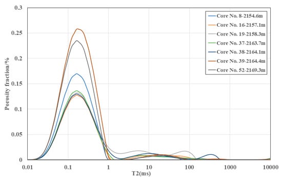
Figure 1.
NMR T2 spectra of core plugs at different depths under fully water-saturated conditions from Well YT1, Lianggaoshan Formation, Sichuan Basin.
Guided by the above core NMR results, we design idealized T2 spectra that better reflect in situ reservoir characteristics by modeling them as superpositions of Gaussian peaks consistent with the geophysical meaning of shale-oil reservoirs in the Lianggaoshan Formation. First, we define the T2 relaxation axis on a logarithmically uniform grid from 0.01 to 1000 ms with 64 log-spaced points.
Next, we assume the T2 spectrum is a sum of multiple Gaussian peaks. Each peak takes the form
where fj is the T2 amplitude at the j-th grid point (dimensionless); wi is the weight (relative amplitude) of the i-th Gaussian peak; μi is the center of the i-th peak on the logarithmic T2 axis (ms); and is its (dimensionless) variance controlling peak width.
By adjusting peak positions, amplitudes, and widths (Table 1), we can emulate diverse T2 distributions that reflect different geological settings and petrophysical conditions.

Table 1.
Parameter settings for different T2 spectrum types.
To reflect porosity characteristics of shale-oil reservoirs, the Gaussian mixture is normalized and then scaled by porosity:
where ϕ is the formation porosity (%) and ϕj is the porosity contribution at the j-th T2 bin (%).
In Figure 2a, we illustrate single-, bi-, and tri-modal spectra. For the single-peak case, the peak is set at 0.2 ms with width σ = 0.3 and weight w = 1. For the bi-modal case, the left peak is at 0.2 ms (σ = 0.3, w = 0.8) and the right peak at 5 ms (σ = 0.2, w = 0.2). For the tri-modal case, peaks are at 0.2 ms (σ = 0.3, w = 0.7), 5 ms (σ = 0.2, w = 0.2), and 100 ms (σ = 0.2, w = 0.1). The porosity is set to 5%. The relaxation-time range spans 0.01–1000 ms with N = 64 log-spaced grid points. Each peak corresponds to different pore-fluid populations: short-T2 peaks generally indicate bound water, whereas long-T2 peaks indicate free fluids. Using the generated ideal T2 spectra and the discrete forward model in Equation (6), we compute the corresponding NMR decay signals (Figure 2b) with an echo spacing of 0.2 ms.
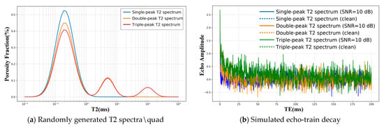
Figure 2.
Example of a randomly generated bi-/tri-modal T2 spectrum and its corresponding echo train.
To substantially enhance model generalization during dataset construction, we introduce a diversity strategy: for each spectrum type, the number of peaks, their positions, amplitudes, and widths are randomly varied within the ranges above; porosity is sampled in 1–10% to match realistic shale-oil reservoirs. Beyond spectral variability, the signal-to-noise ratio (SNR) is drawn uniformly from 5 to 30 (dB) to emulate the high-noise conditions typical of such reservoirs. The dataset is then split into training, validation, and test subsets in a 7:2:1 ratio.
Through this systematic generation and preprocessing workflow, we obtain a high-quality and broadly representative dataset that covers multi-peak structures and a range of noise levels, thereby providing a solid foundation for training and validating the proposed autoencoder-based one-dimensional T2 inversion model.
4. Theoretical Foundation
4.1. Autoencoder Model
In the study of one-dimensional T2 spectrum inversion, the choice of model architecture is directly related to the accuracy and effectiveness of the inversion results. Given the complexity of the inversion problem, an autoencoder is adopted as the primary framework. The autoencoder, with its efficient encoding-decoding mechanism, can extract deep features from the input echo train and subsequently reconstruct the corresponding T2 spectrum.
The basic structure of the autoencoder consists of two parts: the encoder and the decoder [16]. The primary task of the encoder is to map high-dimensional input data into a lower-dimensional latent space, capturing the main features within the data. The decoder, on the other hand, is responsible for reconstructing the T2 spectrum from this latent representation in a manner that closely approximates the original output. This design approach aligns with the goal of T2 spectrum inversion, which is to extract key physical information from complex echo trains.
Mathematically, the encoding and decoding processes can be expressed as:
Here, x represents the input signal, z is the latent representation, is the reconstructed output, W and b are the weight matrix and bias term, respectively, and σ is the activation function.
During the training process of the autoencoder, the choice of loss function is crucial for the model’s performance. Traditionally, the autoencoder uses Mean Squared Error (MSE) as the loss function, which is expressed as follows:
Here, N is the number of samples, xi represents the input data, and is the reconstructed data output by the model. Mean Squared Error (MSE) calculates the squared difference between the model’s output and the actual input, aiming to minimize the distance between the predicted values and the true values.
MSE is relatively straightforward to implement, easy to understand, and computationally efficient. Additionally, this loss function is continuously differentiable, facilitating the use of optimization algorithms such as gradient descent for training. However, MSE is sensitive to outliers, which can interfere with the model during training and affect overall performance. Furthermore, when dealing with sparse data, MSE may not effectively capture important features, leading the model to overlook key information during learning.
The application of autoencoders in T2 spectrum inversion is theoretically feasible. First, there exists a nonlinear relationship between the echo train and the T2 spectrum, which the nonlinear activation mechanisms of autoencoders can effectively capture. Second, the essence of the T2 spectrum inversion task is to extract useful information from sparse data; the design of the latent layer in the autoencoder allows for compressing the input data into a lower dimension, removing redundant information and thereby enhancing the accuracy of the inversion.
4.2. Wavelet Transform
The wavelet transform is a method that provides localized information in both the time and frequency domains, making it particularly suitable for processing signals with non-stationarity and local characteristics. The wavelet transform decomposes the signal using a set of waveforms (i.e., wavelets) of different scales and positions, effectively capturing variations in multiple frequency components. The mathematical expression of the wavelet transform is:
where Wa,b(t) is the wavelet coefficient of the signal x(t) at scale a and position b, reflecting the characteristics of the signal at different scales and time positions. x(τ) is the time-domain signal, representing the collected echo series, with τ as the time variable. ψ is the mother wavelet, indicating the scaling and translation at time position t, while a is the scaling factor that controls the width of the wavelet, affecting the time and frequency resolution. The expression represents the integral over time τ to compute the wavelet coefficients of the signal at various scales and positions. Through the wavelet transform, subtle features of multi-exponential decay in the echo series can be extracted.
4.3. Design of Loss Function Based on Self-Attention Mechanism
The self-attention mechanism dynamically adjusts the weights of input features, allowing the model to focus more on important information when dealing with sparse features. This mechanism is particularly crucial in the T2 spectrum inversion task, as the T2 spectrum has most of its values being very small except for the peaks. The self-attention mechanism can help the model ignore these smaller values and concentrate on the features of the non-zero values. To achieve this, a custom weighted mean squared error loss function (Weighted Mean Squared Error, WMSE) is used to optimize the training process of the model. First, the basic mean squared error (MSE) is calculated, expressed as follows:
Next, a threshold is set to distinguish between important features and noise. The true values are first evaluated against this threshold to obtain the weights, expressed as follows:
Here, points greater than the threshold are assigned a weight of 1, while the weights for other points are set to 0. For points below the threshold, a smaller weight (0.1) is assigned, calculated as follows:
By combining the two types of weights, a composite error is formed:
This allows weightstotal to effectively differentiate between important features and small-value features. The final weighted loss is calculated as follows:
Here, ϵ is a small constant used to prevent division by zero.
In this process, the design of the weighted_loss allows the model to focus more on important non-zero features during training while suppressing the influence of noise, thereby improving the inversion results.
5. Experimental Design and Result Analysis
In the initial training phase of the model, a standard autoencoder architecture was employed to perform T2 spectrum inversion. The main structure of the model consists of an input layer, hidden layers, and an output layer, with network parameters set as shown in Figure 3 and Table 2. The input feature dimension, representing the number of extracted echo features, was set to 500; the output layer dimension was configured differently from a traditional autoencoder, set to 64 to reconstruct the original T2 spectrum.
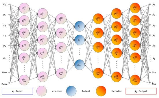
Figure 3.
Architecture of the autoencoder network.
Table 2.
Autoencoder Network Architecture.
To prevent overfitting during training, the Dropout technique was introduced. Dropout is a regularization method that randomly “drops out” a portion of neurons during training to reduce co-adaptation among neurons [17]. This strategy effectively enhances the model’s generalization ability, allowing it to perform more robustly on unseen samples. In each training iteration, Dropout randomly selects a certain proportion of neurons and sets their output to zero, thereby forcing the model to learn more robust feature representations.
In the hidden layers, the Leaky ReLU activation function is used. Unlike traditional ReLU, Leaky ReLU has a small slope when the input is less than zero, which helps mitigate the “dying ReLU” problem. Its formula is as follows:
In this context, α is set to 0.01. The use of Leaky ReLU aims to accelerate the convergence process and improve the model’s performance during training.
Root Mean Square Propagation (RMSprop) is a commonly used adaptive learning rate optimization algorithm, particularly suitable for optimizing problems with non-stationary targets. When training deep neural networks, RMSprop effectively addresses the issue of improperly set learning rates in traditional gradient descent methods, avoiding convergence that is either too fast or too slow.
The core idea of RMSprop is to maintain a separate learning rate for each parameter and dynamically adjust these learning rates based on past gradient information. Specifically, RMSprop adjusts the update step size for each parameter by calculating the exponentially weighted moving average of the squared past gradients. Its update formula is as follows:
In this context, vt represents the exponentially weighted moving average of the squared gradients. β is the decay rate, set to 0.9. gt is the current gradient, θt denotes the parameters, η is the initial learning rate, and ϵ is a small constant used to prevent division by zero errors.
RMSprop adaptively adjusts the learning rate for each parameter, allowing the model to converge more efficiently during training. This feature makes RMSprop a preferred optimizer for many deep learning tasks, especially when dealing with large-scale and sparse data.
In this study, 10,000 T2 spectra, including single-peak and double-peak cases, were randomly generated based on the constructed autoencoder network model. The generation of these spectra considered diverse features to enhance the model’s generalization capability. Additionally, echo intervals of 0.1 and 0.2 milliseconds were used, with a total of 500 echoes calculated to achieve signal-to-noise ratios (SNR) of 20, 40, 60, 80, and 100, thereby constructing the dataset.
During the training process, the choice of hyperparameters significantly impacts model performance. To ensure the autoencoder’s effectiveness in T2 spectrum inversion tasks, the following hyperparameters were set:
Learning Rate: The learning rate was set to 0.00001. The learning rate controls the step size during model weight updates, and a smaller learning rate helps maintain stability during training, preventing instability caused by rapid updates. Although a lower learning rate may prolong training time, it aids in capturing subtle features when dealing with complex data.
Batch Size: A batch size of 128 was selected. The batch size determines the number of samples used for each weight update. A larger batch can accelerate training and enhance model stability, though it may increase memory consumption. A batch size of 128 provides sufficient randomness while ensuring training efficiency, facilitating better generalization during the training process.
Number of Epochs: The number of epochs was set to 1000. Each epoch represents a complete pass through the entire training dataset. Choosing a higher number of epochs allows the model more opportunities to learn the underlying features of the data. However, excessive epochs may lead to overfitting, necessitating monitoring of the validation set’s performance to maintain a balance in generalization capability.
Using the above hyperparameter settings, we trained the autoencoder and plotted the learning curves of training and validation errors (Figure 4). As training proceeds, both errors decrease steadily, indicating progressive improvement in predictive capability. The small gap between the training and validation curves suggests that the dataset is well balanced and that the random split yields subsets with similar distributions. Convergence is rapid: by around 40 epochs the validation RMSE is already low. With further epochs, the RMSprop optimizer adaptively reduces the effective step size, and the model attains a low final error, evidencing stable convergence and satisfactory training performance.
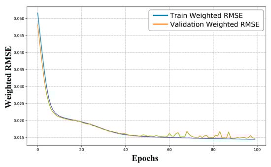
Figure 4.
Training and validation loss vs. epochs for the autoencoder (blue: training loss; orange: validation loss).
Although the conventional autoencoder (AE) yields reasonable preliminary results for T2 spectrum inversion (Figure 5), the reconstructions exhibit oscillatory artifacts and limited accuracy. The model can capture the presence of multiple peaks, but noticeable errors remain due to the spectrum’s complexity. These results indicate that, while a standard AE can succeed in certain cases, it still falls short on complex echo trains—especially those with multiple peak components. In essence, the baseline AE fails to robustly capture multi-peak structure and salient frequency-domain cues in signals with rich structure, which leads to suboptimal inversion accuracy.
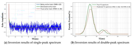
Figure 5.
One-dimensional T2 inversion with the autoencoder—comparison between the true T2 spectrum (blue) and the predicted T2 spectrum (orange). The x-axis is T2 (ms, log scale); the y-axis is normalized amplitude.
Motivated by these limitations, we enrich the model’s input features to improve inversion accuracy. The underperformance of the baseline is attributed to its plain fully connected architecture and the use of raw time-domain echoes alone, which do not fully exploit the multi-exponential decay characteristics of CPMG echo trains. To better expose these characteristics, we apply a discrete Fourier transform (DFT) to convert the time-domain signal to the frequency domain, and then construct a composite feature matrix by concatenating the magnitude spectrum, the phase spectrum, and the original echo train. This hybrid representation is subsequently fed into the AE for training.
Features are derived from the echo-train signal using a Fourier transform (Figure 6) and subsequently employed to invert the T2 spectrum.
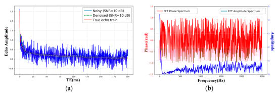
Figure 6.
Echo train and its Fourier-domain representation. (a) Echo train at SNR = 10 dB (blue: noisy echo; green dashed: denoised echo; red: ground-truth echo). x-axis: TE (ms); y-axis: amplitude. (b) Fourier transform of the echo train (blue: magnitude spectrum, right y-axis; red: phase spectrum, left y-axis). x-axis: frequency (Hz).
Figure 6a shows a typical CPMG-style decay corrupted by additive noise (SNR = 10 dB). The denoised trace (green, dashed) follows the true multi-exponential decay (red) and suppresses high-frequency fluctuations visible in the noisy signal (blue). Figure 6b presents the corresponding frequency-domain features: the magnitude spectrum (blue) concentrates energy at low frequencies—consistent with a smooth exponential decay—while the phase spectrum (red) appears erratic due to noise. These Fourier features (magnitude and phase) provide complementary information to the time-domain echo and are subsequently used as inputs to the inversion network.
We form a composite input by concatenating the phase spectrum, magnitude spectrum, and the raw echo train obtained via the Fourier transform. After replacing the original inputs with this hybrid matrix, the learning curves of training and validation errors are shown in Figure 7. As training proceeds, both errors decrease steadily, indicating progressive improvement in predictive capability and suggesting that the randomly split training and validation subsets have similar distributions. The errors approach a plateau around epoch ≈ 400, implying that the Fourier-derived features enable the network to better learn the mapping from echo trains to the T2 spectrum, thereby reducing the final convergence error.
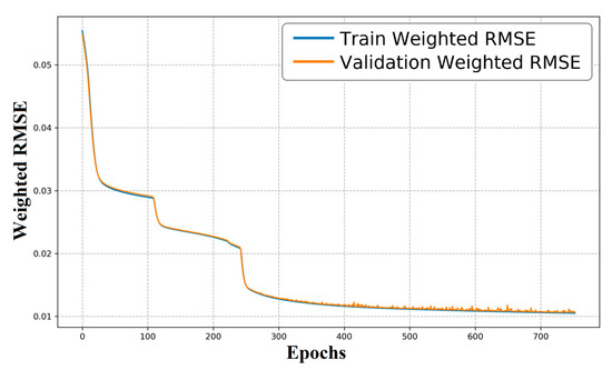
Figure 7.
Learning curves of the autoencoder—training and validation loss versus epochs (blue: training loss; orange: validation loss).
By feeding a time–frequency hybrid input—the raw echo train concatenated with the magnitude and phase spectra from the Fourier transform—the T2 inversion error is markedly reduced (Figure 8): the test RMSE drops from about 10−3 with the plain autoencoder to about 10−6 with the proposed model. This demonstrates that deeper feature mining in the joint time–frequency space substantially enhances the network’s representational capacity and yields more accurate T2 spectra.
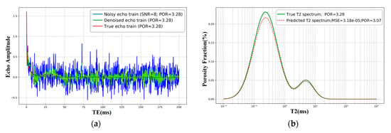
Figure 8.
Effect of Fourier-derived time–frequency features on T2 spectrum inversion. (a) Bi-modal echo train at SNR = 8 (blue: noisy echo; green: denoised echo; red: ground-truth echo). x-axis: TE (ms); y-axis: amplitude. (b) Predicted bi-modal T2 spectrum versus ground truth (green solid: true T2 spectrum; red dashed: model prediction using time–frequency features). x-axis: T2 (ms, log scale); y-axis: porosity fraction (%).
6. Discussion
6.1. Baseline AE with Time-Domain Echoes
Using only the raw echo train as input, the conventional autoencoder (AE) can recover the general shape of the T2 spectrum, including the presence of multiple peaks (Figure 5). However, oscillations and noticeable bias remain for complex, multi-peak cases, reflecting the ill-posed nature of the inverse problem and the limited ability of a plain fully connected encoder to expose multi-exponential structure in the echoes. This translates into moderate accuracy and unstable generalization on harder examples (cf. Figure 4 and Figure 5).
6.2. AE with Fourier-Derived Time–Frequency Features
After concatenating the magnitude spectrum, phase spectrum, and the raw echo train into a hybrid input (Figure 6), the learning curves become smoother and the validation error plateaus earlier (≈epoch 400; Figure 7). Qualitatively, the Fourier representation concentrates energy at low frequencies for exponential decays and is robust to small time shifts; together with energy normalization this reduces feature variance across splits. Empirically, the test error drops from ∼10−3 for the plain AE to ∼10−6 with the Fourier-enhanced model (Figure 8), indicating a clear gain in reconstruction fidelity for single- and bi-modal spectra.
6.3. Effect of the Sparsity-Aware Weighted Loss
Replacing plain MSE with a sparsity-aware weighted loss that down-weights long zero-valued T2 bins and emphasizes peak regions improves peak fidelity and accelerates convergence (Section 4.3). Advantages include mitigation of severe class imbalance and better reconstruction of narrow peaks; disadvantages are potential under-fitting of the baseline and sensitivity to over-aggressive thresholds, which we control by bounding weights and validating hyperparameters. Note this is not a transformer-style attention; it is a deterministic, data-dependent reweighting aligned with the physics of sparse T2 spectra.
6.4. Decision Rationale and Scenario Mapping
Low–moderate SNR, multi-exponential decays: AE + Fourier hybrid input + sparsity-aware loss → most stable validation and highest fidelity (Figure 6, Figure 7 and Figure 8).
Overall, these outcomes justify adopting the AE with Fourier-derived features plus sparsity-aware weighting as the default pipeline for 1D T2 inversion in shale-oil settings.
7. Conclusions
In summary, this study develops an autoencoder- and Fourier-transform-based inversion method for shale oil T2 spectrum, which improves inversion accuracy, robustness against noise, and computational efficiency. The main conclusions are as follows:
1. Feasibility and dataset. We formulate the NMR forward model S = Kf and construct a representative synthetic dataset—anchored to shale-oil core observations—covering single- and bi-modal T2 spectra and realistic noise levels (e.g., SNR = 5–30). This enables controlled, systematic evaluation of deep models for one-dimensional T2 inversion.
2. Baseline limitation. A plain time-domain autoencoder (AE) recovers the overall spectral shape but exhibits oscillations and bias on complex, multi-peak cases, revealing the need for richer input features.
3. Main finding. Concatenating Fourier magnitude and phase spectra with the raw echo train markedly improves accuracy and stability: the test error decreases from ∼10−3 to ∼10−6 and the validation curves plateau earlier and more smoothly.
4. Loss design. A sparsity-aware weighted loss that emphasizes peak regions while down-weighting long zero-valued bins further enhances peak fidelity and convergence; bounding the weights mitigates potential trade-offs.
5. Implication. The combined AE + Fourier features + sparsity-aware loss pipeline provides a practical and robust route for 1D T2 spectrum inversion under shale-oil conditions and offers a solid foundation for extension to 2D spectra in future work (e.g., integrating physics-guided constraints and broader field validation).
Author Contributions
All authors contributed to the study conception and design. S.J., J.Z. and L.B. wrote the main manuscript. B.X. and Y.C. analyzed the data. Z.W. and S.Z. prepared figures. All authors have read and agreed to the published version of the manuscript.
Funding
This paper is funded by the CNPC-SWPU Innovation Alliance (2020CX010204) and Sichuan Provincial Natural Science Foundation (2023NSFSC0259), and supported by State Key Laboratory of Oil and Gas Reservoir Geology and Exploitation, Southwest Petroleum University, the views expressed are authors’ alone.
Institutional Review Board Statement
Not applicable.
Data Availability Statement
All data generated or analyzed during this study are included in this published article.
Conflicts of Interest
Authors Li Bai, Bing Xie, and Shaomin Zhang are employed by PetroChina Southwest Oil and Gas Field Company. The remaining authors declare that the research was conducted in the absence of any commercial or financial relationships that could be construed as a potential conflict of interest.
References
- Sun, Z.; Li, Z.; Shen, B.; Zhu, Q.; Li, C. NMR technology in reservoir evaluation for shale oil and gas. Pet. Geol. Exp. 2022, 44, 930–940. [Google Scholar] [CrossRef]
- Trbovic, N.; Smirnov, S.; Zhang, F.; Brüschweiler, R. Covariance NMR spectroscopy by singular value decomposition. J. Magn. Reson. 2004, 171, 277–283. [Google Scholar] [CrossRef] [PubMed]
- Prammer, M.G. NMR Pore Size Distributions and Permeability at the Well Site. In Proceedings of the SPE Annual Technical Conference and Exhibition, New Orleans, LA, USA, 25–28 September 1994. [Google Scholar]
- Ge, X.; Wang, H.; Fan, Y.; Cao, Y.; Chen, H.; Huang, R. Joint inversion of T1–T2 spectrum combining the iterative truncated singular value decomposition and the parallel particle swarm optimization algorithms. Comput. Phys. Commun. 2016, 198, 59–70. [Google Scholar] [CrossRef]
- Weng, A.; Li, Z.; Mo, X.; Lu, J. On high resolution inversion of NMR logging data. Well Logging Technol. 2002, 26, 455–463. [Google Scholar]
- Jiang, R.; Yao, Y.; Miao, S.; Zhang, C. Improved algorithm for singular value decomposition inversion of T2 spectrum in nuclear magnetic resonance. Editor. Off. ACTA Pet. Sin. 2005, 26, 57–59. [Google Scholar]
- Butler, J.P.; Reeds, J.A.; Dawson, S.V. Estimating solutions of first-kind integral equations with nonnegative constraints and optimal smoothing. SIAM J. Numer. Anal. 1981, 18, 381–397. [Google Scholar] [CrossRef]
- Lin, F.; Wang, Z.; Li, J.; Zhang, X. Study on algorithms of low SNR inversion of T2 spectrum in NMR. Appl. Geophys. 2011, 8, 233–238. [Google Scholar] [CrossRef]
- Venkataramanan, L.; Gruber, F.K.; Habashy, T.M.; Freed, D.E. Mellin transform of CPMG data. J. Magn. Reson. 2010, 206, 20–31. [Google Scholar] [CrossRef] [PubMed]
- Venkataramanan, L.; Habashy, T.M.; Freed, D.E.; Gruber, F.K. Continuous moment estimation of CPMG data using Mellin transform. J. Magn. Reson. 2012, 216, 43–52. [Google Scholar] [CrossRef] [PubMed]
- Ge, X.; Wang, H.; Fan, Y.; Cao, Y.; Chen, H.; Huang, R. Joint inversion of T1–T2 spectrum combining iterative TSVD and a parallel particle swarm optimization algorithm. Comput. Phys. Commun. 2016, 198, 59–70. [Google Scholar] [CrossRef]
- Salazar-Tio, R.; Sun, B. Monte Carlo Optimization-Inversion Methods for NMR. Petrophysics 2010, 51, 208–218. [Google Scholar]
- Xiao, L.-Z.; Zhang, H.-R.; Liao, G.-Z.; Fu, S.-Q.; Li, K. Inversion of NMR relaxation in porous media based on Backus–Gilbert theory. Chin. J. Geophys. 2012, 55, 3821–3828. [Google Scholar]
- Arasram, T.; Daoud, R.; Xiao, D. T2 analysis using artificial neural networks. J. Magn. Reson. 2021, 325, 106930. [Google Scholar] [CrossRef] [PubMed]
- Luo, G.; Xiao, L.; Luo, S.; Liao, G.; Shao, R. A study on multi-exponential inversion of nuclear magnetic resonance relaxation data using deep learning. J. Magn. Reson. 2023, 346, 107358. [Google Scholar] [PubMed]
- LeCun, Y.; Bengio, Y.; Hinton, G. Deep learning. Nature 2015, 521, 436–444. [Google Scholar] [CrossRef] [PubMed]
- Srivastava, N.; Hinton, G.; Krizhevsky, A.; Sutskever, I.; Salakhutdinov, R. Dropout: A simple way to prevent neural networks from overfitting. J. Mach. Learn. Res. 2014, 15, 1929–1958. [Google Scholar]
Disclaimer/Publisher’s Note: The statements, opinions and data contained in all publications are solely those of the individual author(s) and contributor(s) and not of MDPI and/or the editor(s). MDPI and/or the editor(s) disclaim responsibility for any injury to people or property resulting from any ideas, methods, instructions or products referred to in the content. |
© 2025 by the authors. Licensee MDPI, Basel, Switzerland. This article is an open access article distributed under the terms and conditions of the Creative Commons Attribution (CC BY) license (https://creativecommons.org/licenses/by/4.0/).