Abstract
Existing methods for estimating formation boundaries from well-log data only analyze the formation along the wellbore, failing to capture changes in the 3D formation structure around it. This paper presents a method for real-time 3D formation boundary interpretation using readily available well logs and seismic image data. In the proposed workflow, the mean formation boundary is estimated as a curve following the well path. 3D surfaces are then fitted through this boundary curve, aligning with the slopes and features in the seismic image data. The proposed method is tested on both synthetic and field datasets and illustrates the capabilities of accurate boundary estimation near the well path and precise representation of boundary shape changes further away from the well trajectory. With this fully automated geological interpretation workflow, human bias and interpretation uncertainty can be minimized. Subsurface conditions can be continually updated while drilling to optimize drilling decisions and further automate the geosteering process.
1. Introduction
The oil and gas industry faces a dual challenge: drilling more efficiently while maximizing production. To address this, geosteering emerged as a critical technology, which involves precise control and adjustment of drilling operations to navigate through subsurface geological formations with accuracy and efficiency [1,2,3,4,5]. This transformative technology has revolutionized well drilling and reservoir management [6], resulting in reduced operational costs, optimized hydrocarbon production, and a minimized environmental footprint.
Geosteering, aiming at intersecting specific reservoir zones, can be dissected into three key components: predrilling planning, monitoring/model updating, and in-drilling decision-making [7]. As the cornerstone of successful geosteering, geological interpretation involves continuous measurement, interpretation, and modeling of the formation of interest, drawing from various data sources like well-log measurements, seismic surveys, cuttings, and coring operations [8]. More specifically, during the construction of the well, geoscientists and drilling engineers frequently analyze the collected well logs to determine lithology and resistivity of the formations surrounding the wellbore while drilling (well-log interpretation) and combine the interpretation with established larger-scale area seismic surveys to reconstruct the subsurface formation shapes (horizon tracking). The interpreted formation shapes need to be continually updated while drilling to offer real-time insights into subsurface conditions, which help drillers make informed geosteering decisions to optimize the drilled well trajectory and well placement.
However, nowadays, processes in these different phases of geosteering highly rely on human inputs, initial condition setups, and personal judgments, which can lead to suboptimal and biased drilling decisions. Moreover, given the indirect and incomplete information used in geological interpretation, uncertainties are unavoidable [9]. Recent research has focused on probabilistic well-log interpretation techniques to address the uncertainty in geological interpretation. One prominent approach is to interpret the well-log data via Bayesian analysis. Traditional Kalman filters, ensemble Kalman filters, and Monte Calo techniques have been explored to generate probabilistic near-wellbore formation shapes. An alternative approach is to treat the interpretation as a large-scale statistical inference problem, which is generally of high dimensionality and is computationally intensive.
In geological interpretation, the wellbore itself (and the high resolution well logs taken in and around it) is only a minute feature in the entire subsurface volume that is of interest to well construction operations. To be of practical use, well-log interpretation must be interpreted in the context of a larger scale model, which in the field often comes from a seismic survey taken over a large area [10], to accomplish the horizon tracking of subsurface formation shapes. Algorithms have been proposed to auto-track the horizon within the 3D seismic volume, and recently advanced data processing approaches are incorporated to improve the tracking accuracy and efficiency.
In this paper, we delve into the prediction and reconstruction of both near-wellbore and geological-area formation shapes, considering the uncertainty and various operational constraints of geological interpretation and geosteering in well construction. A fully automated workflow is proposed to combine well-log interpretation and horizon tracking to optimize geosteering activities. The implementation of recursive Bayesian filter for formation shape estimation is first explored. Additionally, the concept of horizon auto-tracking (a numerical algorithm for formation horizon identification in the 3D space) is introduced. Combing well logs and initial structural geomodels, it yields a stereoscopic data for geosteering process. Lastly, the proposed geosteering interpretation approach is rigorously tested, using both synthetic and field datasets, to validate its effectiveness and reliability in geosteering applications.
2. Bayesian Well-Log Interpretation
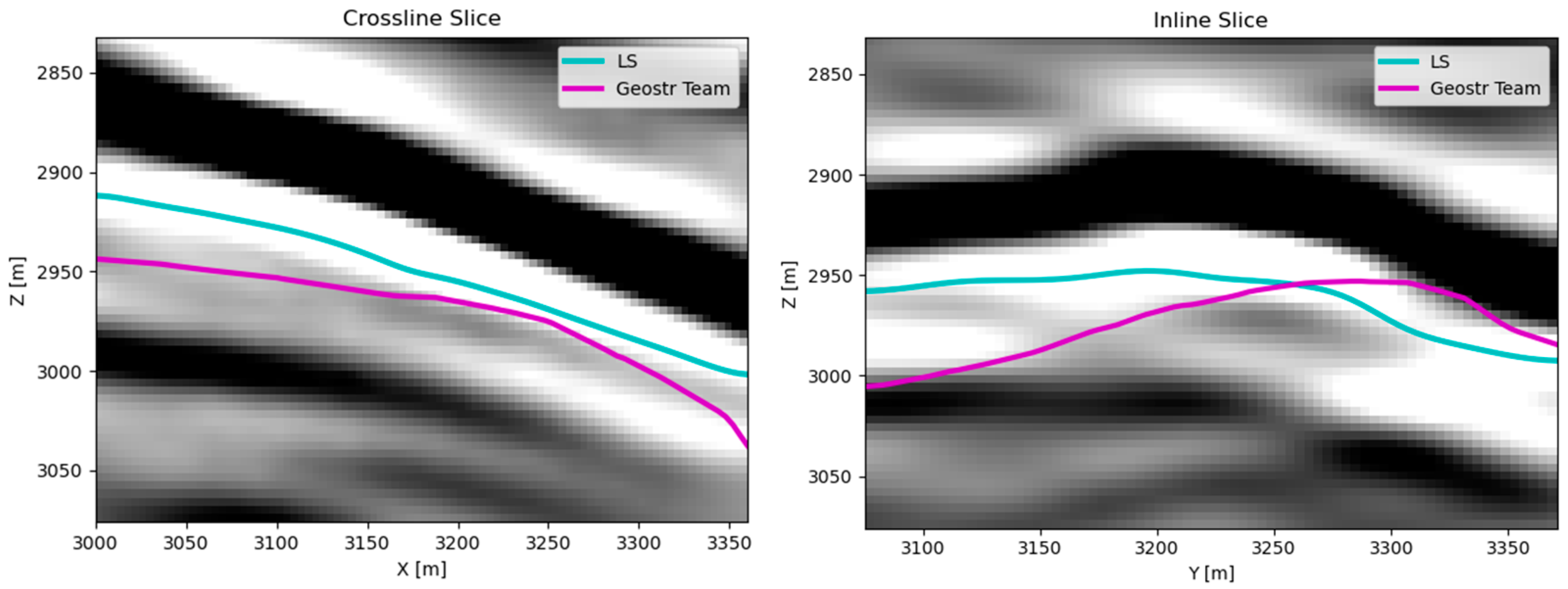
In the well-log interpretation process, the near-wellbore formation shapes are estimated by pattern-matching between the measured and modeled logging tool responses [8,11]. More specifically, the response of the logging tool is firstly modeled as a function of its relative location compared to the formation boundary, which is derived from an offset well log or a composite of well logs (a reference or type log). By matching the well log obtained while drilling and the established logging tool response, the near-wellbore formation shape can be reconstructed [10].
There are multiple models to describe the well-log interpretation problem and Figure 1 below provides two examples. One example (Figure 1, left) involves tracking the tool location, either in Cartesian coordinates or in terms of its True Vertical Depth (TVD), inclination, and azimuth [12]. Additionally, it involves monitoring the formation’s dip angle and the fault throw (i.e., sudden vertical displacement) at each location along the wellbore. Another example (Figure 1, right) also employs the logging tool’s location, but instead of considering the dip angle or fault throw, it utilizes the concept of Relative Stratigraphic Depth (RSD) to represent the location of the formation boundary [13].
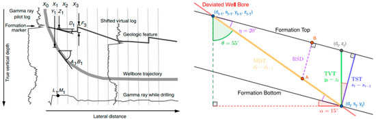
Figure 1.
Geosteering state spaces [10,11].
In the field operation, recursive Bayesian filtering is becoming a common approach used to generate probabilistic geological interpretations for geosteering. One of the earliest examples in the literature is [7], which uses the traditional Kalman filter to estimate the distance to formation boundaries along the lateral section of a wellbore, utilizing resistivity measurements. Resistivity is a common well-log measurement that is produced by the resistivity tool, which uses current flow in a coil to induce current flow in the formation under investigation to measure the formation. Various information, such as formation porosity, water saturation, presence of hydrocarbons, etc., can be inferred from the resistivity well logs. In [14,15,16], the response of a resistivity tool to the formation rock is modeled as an electro-magnetic simulator and the ensemble Kalman filter (EnKF) is adopted to estimate the formation boundaries. More recent publications [13,17,18,19] adopted sequential Monte Carlo techniques (i.e., particle filters) as a substitution of the Kalman filter. However, these aforementioned interpretation techniques only estimate the distance to or shape of nearby formation boundaries in the near-wellbore field. There is no consideration of the formation boundaries far away from the wellbore, which limits the application of the recursive Bayesian filtering for further steering decision optimization.
Other recent well-log interpretation approaches use similar formation boundary models in Figure 1, but unlike recursive Bayesian filters which solve the estimation problem sequentially, they solve a larger-scale inference problem, see [12,20,21]. Given a prior estimate of the formation boundaries (or some representation of the boundaries) along with new measurements taken along the wellbore, these methods infer the posterior distribution of the formation boundaries over the entire wellbore. However, due to the high dimensionality of this problem, the proposed model representations and solution methods are computationally intensive and do not always offer significant improvements over the most efficient recursive Bayesian filtering methods [13].
3. Horizon Auto-Tracking
In the field, tracking of area-scale formation shape and locations starts with seismic surveys, which are taken by shooting sound waves into the geological area of interest and measuring the two-way wave travel time with numerous survey stations. Disparities in rock types and properties can be identified through the reflection pattern of the sound waves. The final seismic surveys are produced by migrating the two-way sound wave travel time to the depth domain via wave propagation models, which are composed of velocity building, seismic tomography, and seismic waveform inversion. Notably, the subsurface wave propagation models are iteratively updated until the misfit between the model predictions and the collected seismic data are minimized. One example of the P-wave velocity model is shown in Figure 2.
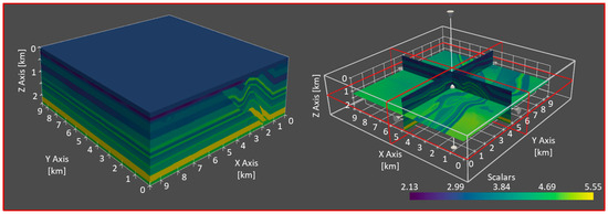
Figure 2.
A 3D P-wave velocity model volume (left) and cross-section (right) taken from the synthetic Overthrust dataset. Changes in color intensity represent changes in P-wave velocity.
More specifically, the subsurface wave propagation model interprets the structure of the formation as a unitless intensity across the volume of interest. As shown in Figure 2 and Figure 3, changes in color/intensity relate to changes in the rock properties and lithology. In practice, this structural model still requires manual interpretations to categorize the sequences of formations and reflective boundaries in the seismic volume to identify the faults (sudden structural discontinuities) and horizons (structural boundaries), which are represented as 2D curves or 3D surfaces, as shown in Figure 4.
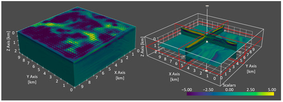
Figure 3.
A 3D seismic image volume (left) and cross-section (right) taken from the synthetic Overthrust dataset. Changes in color intensity represent changes in seismic amplitude in migrated image.
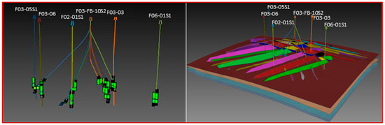
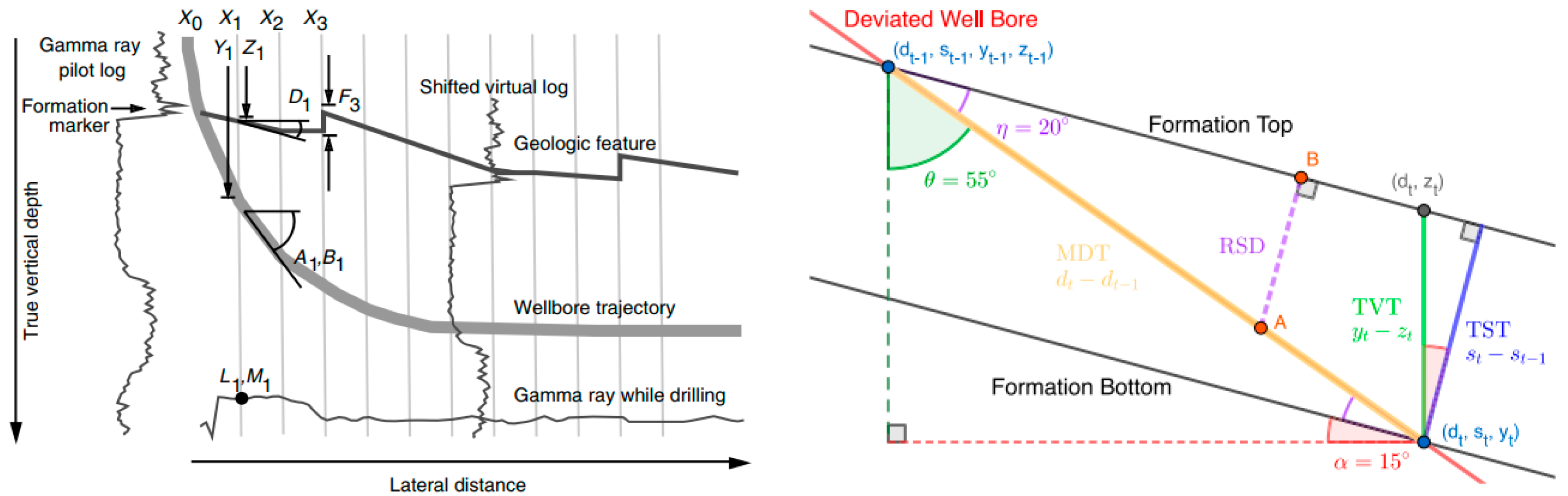
Figure 4.
Wellbore surveys (vertical lines) passing through 3D geomodel horizons (rectangular surfaces) as well as fault geometries (polygons passing through horizons) derived from the seismic model in the synthetic Overthrust dataset.
In the semi-automated process of horizon auto-tracking, the user usually selects a seed or control point within the 3D volume as the starting point. Subsequently, the auto-tracking algorithm automatically identifies well-log features near the seed point (often an amplitude peak) and attempts to trace paths or surfaces through the 3D volume that share similarities in these features [22]. This tracking process continues until the algorithm encounters a discontinuity or exceeds a predefined expansion threshold. The user then reviews and refines the generated horizon shapes and repeats this process for each horizon of interest. More recent versions of these algorithms leverage various comprehensive features within the 3D seismic volume, see [20,22,23,24] and incorporate advanced data processing approaches like deep learning, see [25,26,27,28,29,30].
While this initial structural geomodel serves as a valuable tool for geosteering, it, much like well logs, is insufficient on its own for guiding steering decisions. It is because seismic inversion and depth migration are able to produce a structural model that closely aligns with the measured seismic survey data, but these solutions of the model are non-unique and typically provide low resolutions. Besides, the resulting model is subject to human interpretation and can potentially introduce further errors. Consequently, this initial structural model is treated as an initial hypothesis regarding locations and shapes of formation boundaries and faults. Further refinements and integration with other data sources are necessary for optimized geosteering decisions making.
4. Methods
As discussed in the previous section, while neither well logs nor initial structural geomodels are sufficient on their own to drive real-time geosteering optimization, together they form the basis of real-time geosteering interpretation and decision making. The initial structural model can be used to generate an initial planned trajectory. During the drilling process, the well log is interpreted against one or more offset wells and is adopted to update the formation boundary estimations. In this session, an automated 3D formation boundary interpretation approach, combining well logs and seismic image data, is described in detail.
Similar to the work in [13,19], in this work a particle filter is used to address the well-log interpretation problem. The states of interest are inclination , azimuth , TVD , true stratigraphic thickness (TST) of the formation , and RSD between the logging tool and the upper formation layer of the logging tool at the station . The RSD is the distance between the wellbore and the formation boundary measured in the direction of the formation layer’s TST as shown earlier in Figure 1.
The discrete system dynamics of the tool location are computed using the wellbore survey and minimum curvature method (MCM) to estimate the changes in the tool’s location and orientation. MCM is used to interpolate inclination and azimuth, and TVD between survey stations:
where is the additive Gaussian noise affecting the system dynamics and the subscript indicates that each state’s dynamics function (, , , and ) is associated with a different noise term; is the change in measured depth between points and along the wellbore. The dynamics of the formation boundaries are represented using the Setchell equation [10], which relates the change in measured depth thickness (MDT) along the wellbore to changes in TST of the formation as follows:
where is the dip for the formation and is the strike of the formation. This relationship is illustrated in Figure 1 (right). However, in the example shown in the figure, it is assumed that aligns with , so these terms are not shown. Given a sufficiently small increment of measured depth, the change in RSD can be approximated by the change in TST as:
The system observation equations are given by:
where is the additive Gaussian noise affecting the system observations at time ; is a mapping between RSD and the associated type log responses; and are scale and shift factors, which are often necessary to account for differences between the type log and the MWD log caused by their calibration (or lack thereof); is the predicted log response. Realizations of the filter state vector and measurement vector are:
where is the state vector of the nth particle in the filter at time ; is the overall measurement vector at time .
In [13], the authors proposed the use of expectation maximization or Gibbs sampling to approximate and as static hidden states, which, however, is computationally intensive. Here, an alternative procedure is proposed to estimate these factors. First, the wellbore and type logs are aligned using dynamic time warping. Then, a linear transformation (i.e., ) is fit using the method of least squares to match the magnitude of the type log responses to the MWD log responses. This provides estimates of the and parameters that correct for potential shifting and scaling between the log responses. After estimating the RSD and thickness parameters, the TVD of the upper and lower target formation boundaries, and , respectively, can be found at each point along the wellbore using the following equation:
The particle filtering process makes use of these system equations (Equations (1)–(4), (6)–(9)) and sensor measurements to estimate a discrete, multi-dimensional distribution over the state vector at each point along the wellbore. The particle filter is a parameter free, recursive Bayesian filter [31] and achieves the estimation by maintaining a particle set or a list of state vectors. At each iteration, the filter samples a new set of particles from the prior state vector distribution by applying the dynamics equations to the current set of particles. Each particle is then used to predict the next sensor measurement. The particles are then weighted based on the prediction difference and the weights are normalized to sum of one. This is followed by a process known as resampling in which the particle set is replaced by a random sampling from the current distribution and the sampling probability of each particle is equal to its normalized weight value. This new set is the posterior distribution of particles at the current time step (i.e., the current state vector probability distribution).
In the proposed approach, Augmented Monte Carlo Localization (AMCL) and Kullback–Leibler divergence (KLD) sampling [31] are also utilized for improvements against classical particle filters. AMCL helps to prevent degeneracy of the particle set, which is commonly due to repeated resampling. It randomly replaces old particles in the set with random samples from the support of the state space (i.e., the set of feasible values of particle states). Meanwhile, KLD sampling adaptively increases/decreases the size of the particle set to reduce the error in the particle set’s estimation of the target distribution. This helps to keep the filter both accurate and efficient as it always uses a sufficient number of particles.
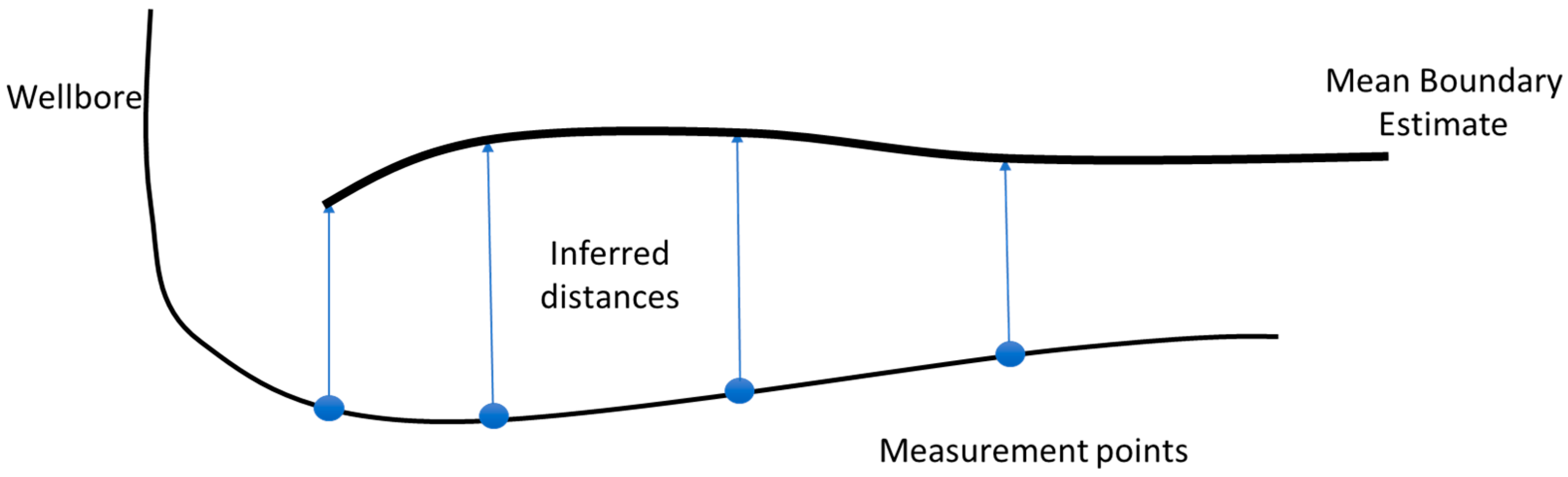
The particle filtering method described above provides an estimate of the RSD separating the wellbore and one or more formation boundaries. Since this analysis is only performed using the one-dimensional log measurement taken along the wellbore, the boundaries lie along a two-dimensional surface following the wellbore as shown in Figure 5.
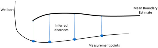
Figure 5.
Illustration of the formation boundary curve estimated along the wellbore.
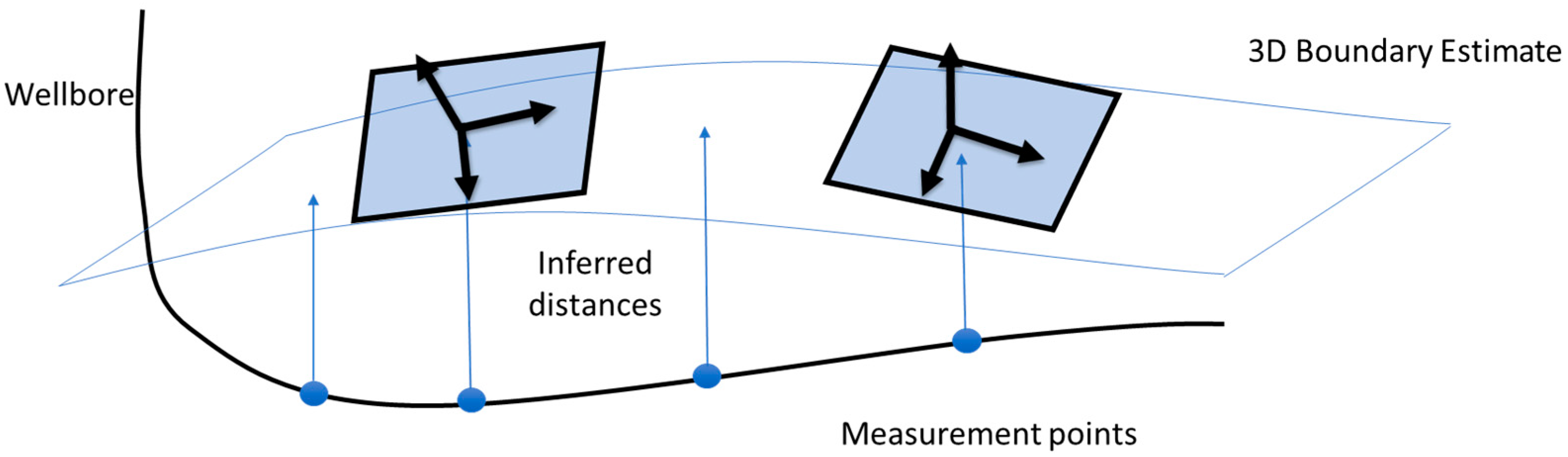
In the 3D formation boundary estimation, boundary points estimated above by the particle filter are used as control points for the horizon tracking algorithm [32]. A 3D surface is approximated conforming to the structure present in the seismic image as illustrated in Figure 6. In this process, the assumption of 2D boundary continuity produced from the particle filter is removed and a surface that conforms to the near-wellbore interpretations made by the particle filter and that follows the seismic formation structure further from the wellbore is tracked. More specifically, careful consideration is required when interpreting through faults or unconformities [33] and in this work a horizon across the entire seismic volume is tracked using a constrained, least-squares method.
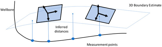
Figure 6.
Illustration of the 3D formation boundary surface estimated across seismic image through the estimated boundary curve.
Similar to how a grayscale picture image is a set of intensity values on a uniform 2D grid, a seismic image is a set of intensity values defined along a uniform 3D grid. The changes in these intensity values represent the structural layout of the subsurface formations and a surface or horizon is represented as a collection of depth with an entry , for every location along the seismic grid. It is also convenient to refer to the set of control points as another collection of depth values , containing the depth value associated with each control point’s grid location.
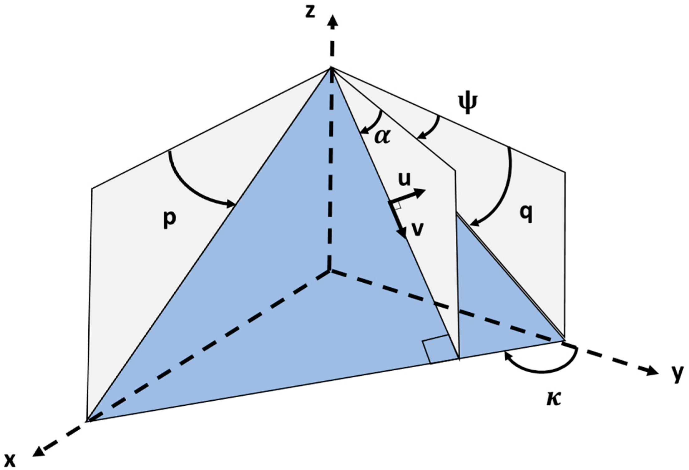
As shown in Figure 7, the seismic reflector slopes, denoted as and , also referred to as inline and crossline dip values, are computed at each point within the seismic image volume using the structure tensor :
where represent the components of the image gradient vector computed within the neighborhood of a point in the 3D image; ⟨∙⟩ signifies a weighted sum of the contents within the brackets. In practice, this convolution operation is often performed using Gaussian smoothing techniques and the eigen decomposition of the structure tensor provides an estimate of the orientation vectors of the seismic reflector surfaces:
where and are the normalized eigenvectors of ; and are the eigenvalues of . Assuming , then is the normal vector to the seismic reflector surface while and are tangent vectors pointing along the surface. The computation of seismic reflector slopes can be derived from the components of the as:
where are the vertical, inline, and crossline components of the vectors in , respectively, and the dip azimuth can be calculated as:
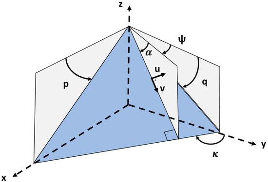
Figure 7.
Seismic reflector surface and its orientations.
The eigenvalues and can also be used to derive the local horizon planarity , which is a value between zero and one and is high near planar regions of the formation and low near discontinuities or faults [34,35]:
In the horizon tracking algorithm, a horizon is assumed to follow the structure of the seismic image when the derivatives and at the associated 2D coordinate follow the corresponding seismic reflector slopes:
where and denote the seismic reflector slopes and computed at the 3D coordinate . In practical scenarios, this assumption is likely to be violated, especially near faults or discontinuities in the seismic image. To address this issue, the relationship described above is weighted by a measure of local planarity, denoted as . Additionally, due to the presence of noise in the seismic image, it may be necessary to regularize the least-squares problem using a small constant, :
Based on Equations (12)–(20), the least-squares method seeks to determine the horizon , that adheres to the slopes within the seismic image, which can be expressed in matrix form as follows:
where and are the matrix representations of the finite-difference approximations of the 2D gradient and Laplace (i.e., second-order gradient) operators, respectively; is a diagonal matrix containing the weights ; is a vector concatenated by reflection slopes and for ; is the constraint enforcing that the surface must pass through the control points defined by the well logs; subscripts and indicate the dependence of the problem on the current or ith estimate of the horizon (). Every time solving the problem yields a new estimate of the surface and this iteration process is necessary because the weighting term and reflection slopes depend on the unknown vector .
This least-squares problem is solved iteratively from an initial guess using the preconditioned conjugate gradient method until the change in the surface estimate between iterations converges below a fixed tolerance. Preconditioned conjugate gradient is ideal for this problem because it allows the constraints to be enforced through the preconditioner matrix and because the system of equations being solved is large and very sparse [32]. The initial guess is found using a nearest-neighbor extrapolation of the depth values of the control points at each location along the seismic image grid (i.e., the nearest control point’s value becomes the initial guess for the value at each point along the seismic image grid).
In conclusion, with the proposed well-log interpretation and horizon tracking algorithm, the geosteering interpretation workflow is illustrated in Figure 8. The workflow can be repeated whenever new log and survey measurements become available.
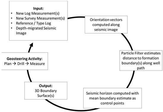
Figure 8.
Seismic reflector surface and its orientations.
5. Test Cases and Results
In this section, the geosteering interpretation workflow described in the previous section is evaluated on both synthetic and field datasets. The synthetic test is performed on the Overthrust dataset [36] in which the interpretations are compared against ground truth information. The field test is performed on the Volve dataset [37] in which the interpretations provided by the proposed approach are compared against the geosteering team’s interpretations over a volume of 200 200 200 m.
The following procedure is followed when testing the proposed geosteering interpretation method. Firstly, an offset well log is converted to the RSD domain. The conversion is based on the well selected by the geosteering team (i.e., the point along the well path where the formation boundary is intersected), which is an event in the seismic model in the synthetic test case and the upper Hugin formation boundary in the Volve test case. Secondly, the particle filter is initiated with an estimate of the wellbore TVD and formation boundary RSD as mean values and small standard deviations. Then, the filter is updated in one-foot intervals along the well path, at which next well-log measurement is fed to the filter and the probability distribution for the wellbore TVD and formation boundary RSD. Lastly, the last 100 m of the boundary curve is used to track a horizon through the seismic image.
5.1. Synthetic Test Case
The Overthrust dataset is a synthetic seismic survey for which both the true seismic velocity model and the seismic image are available, which makes it a popular choice for testing new seismic analysis workflows. For the test of the proposed geosteering interpretation approach, a horizontal wellbore and a vertical offset well are superimposed over a seismic event in the velocity model. As illustrated in Figure 9, both the well paths are plotted against a slice of the seismic volume.
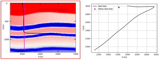
Figure 9.
Wellbore placements against seismic velocity model for synthetic test case in a side view (left) and a top view (right).
In the well-log interpolation process, the velocity model is resampled along both the well paths, where the data collected along the horizontal wellbore serves as the MWD log and the data collected along the vertical offset well serve as the type log in this test simulation. Besides, Gaussian noise with a mean value of zero and variance of 0.1 is added to both sets of sampled data and the seismic event in the velocity model is used to define a ground truth boundary. Both the simulated MWD log and type log are then fed into the particle filter in one-foot increments and the interpolation results are shown in Figure 10. In Figure 10 (and the following Figure 11 and Figure A1), the mean of the boundary prediction distribution is plotted as a black dotted line, and a set of 100 samples from the distribution is plotted as red dots (note that the number of particles used by the filter is not constant as it uses KLD resampling to adaptively decide how many particles to use). The red dots represent the particle filter’s uncertainty around the mean estimate of the formation boundary. After the boundary curve is estimated, the mean absolute error between the mean boundary curve and the final interpretation made by the geosteering team is calculated.
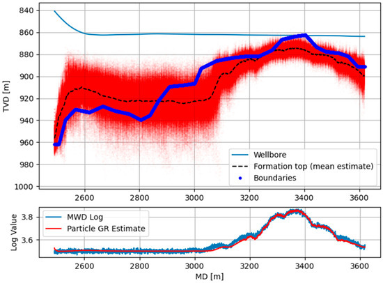
Figure 10.
Formation boundary estimation for synthetic test case.
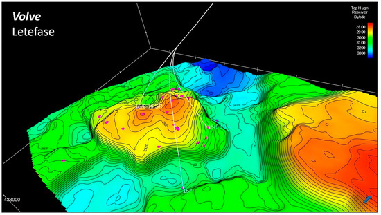
Figure 11.
The upper Hugin boundary in the Volve field dataset [37].
It can be observed from the comparison between the ground truth boundaries and the filter’s prediction in the synthetic dataset that the proposed well-log interpretation algorithm achieves high correlation with the MWD log and infers a reasonable estimate of the seismic boundary. In the example shown in Figure 10, the most difficult region for prediction is from 2600 to 3000 m (~9000 to 10,000 ft), during which the log measurement stops being informative (i.e., the formation boundary is changing, but the investigation depth of the “log” measurement does not pick up the change). Accordingly, the uncertainty in the filter becomes large in this depth region. Once the log starts changing, the uncertainty of the filter’s prediction decreases, and the filter once again starts tracking the formation boundary. In this test case, the mean absolute error for the mean estimate of the formation top is 11.9 m and the Pearson-R score is 0.99.
Following the boundary estimation, the least-squares horizon tracking method is applied to fit a surface through the interpretated boundary and following the orientations of the seismic image. The final horizon tracking result is shown in Figure 12, where we can observe that the identified horizon follows the changes in both the seismic velocity model and image closely.

Figure 12.
3D horizon estimate (green) plotted against orthogonal slices of the seismic velocity model (seismic color map).
5.2. Field Test Cases
The Volve field dataset is a publicly available dataset released by Equinor in 2018 [37]. The dataset contains information collected during the exploration, drilling, and production of the Volve field off the coast of Stavanger, Norway, and contains all subsurface and production data. The Volve field is located five kilometers north of the Sleipner Øst field with water depths of 80 m in the block 15/9 and was in production from 2008 to 2016. The oil was produced from sandstone in the Late Middle to Early Upper Jurassic Hugin Formation with the reservoir located at depths ranging from 2750 m to 3120 m TVD. In this field test case of the proposed geological interpretation workflow, the primary focus is on the following data:
- 3D depth-migrated seismic image
- Geological interpretations
- o
- Formation boundary interpretations
- o
- 3D horizon interpretations (depth-migrated)
- o
- Fault interpretations
- o
- Well picks
- Composite well-log data
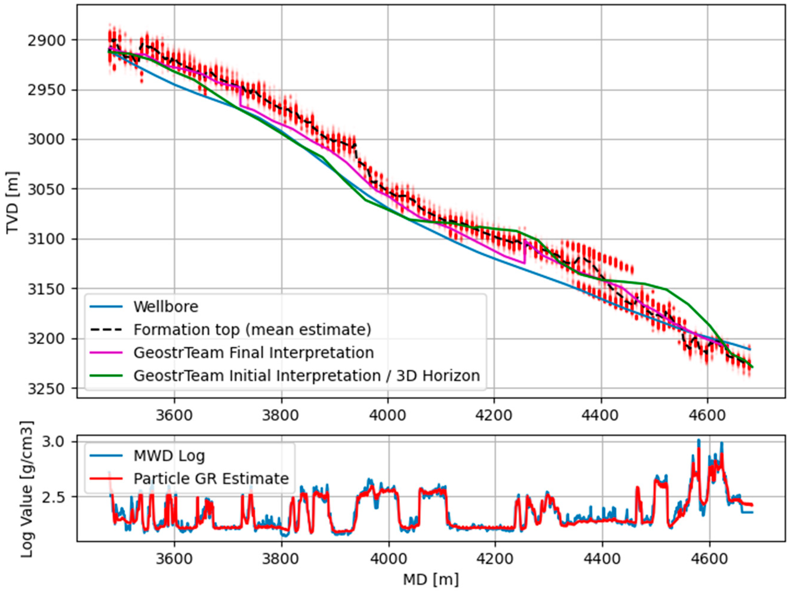
More specifically, the test data adopted for the proposed geosteering interpretation are from two wells in the Volve field dataset, namely 15-9-F-15D (a production well) and 15-9-F-1C (a water injection well). Since ground truth formation boundaries are not available in the Volve field dataset, the geosteering team’s interpretations are used for comparison, which are extracted from the final well placement reports. In addition, although multiple well logs are present in the dataset, the primary log used for this interpretation is the density log. In well 15-9-F-15D, only the upper Hugin boundary (Figure 11) is estimated, which is because the wellbore did not penetrate low enough for the logging tools to gather sufficient information to estimate the base Hugin boundary.
In well 15-9-F-15D, the particle filter is run at each log measurement point, and the results are plotted in Figure 13. It can be observed that the filter estimates closely match both the density log and the geosteering team’s interpretations. A similar comparison between the proposed approach and field results in well 15-9-F-1C is plotted in Figure A1 in the Appendix A.

Figure 13.
Formation boundary estimation for well 15-9-F-15D.
A summary of the testing results for well 15-9-F-15D and 15-9-F-1C are presented in Table 1. In conclusion, the particle filter is always able to find boundaries that correlate well with the MWD log. However, there exist some discrepancies between the particle filter’s estimate and the geosteering team’s interpretations. Some of the variance can be attributed to the difference between the interpolation criterion by human and by algorithm. Another source of deviation is that the proposed interpolation approach only uses the averaged density log from one single offset wellbore, whereas the geosteering team’s interpretations considered multiple offset wells along with azimuthal gamma ray, density, and resistivity logs for each.

Table 1.
Summary of interpretation results.
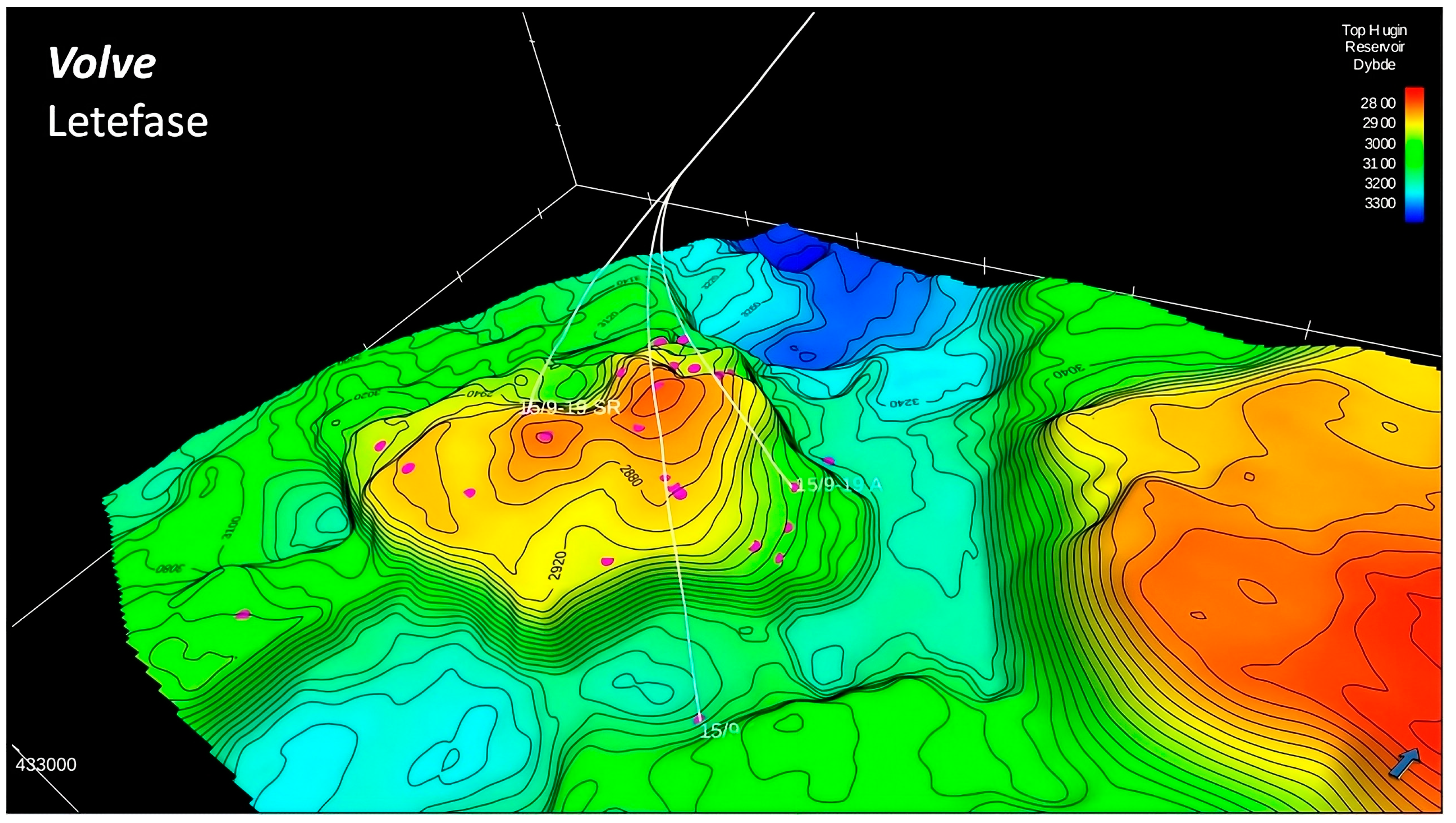
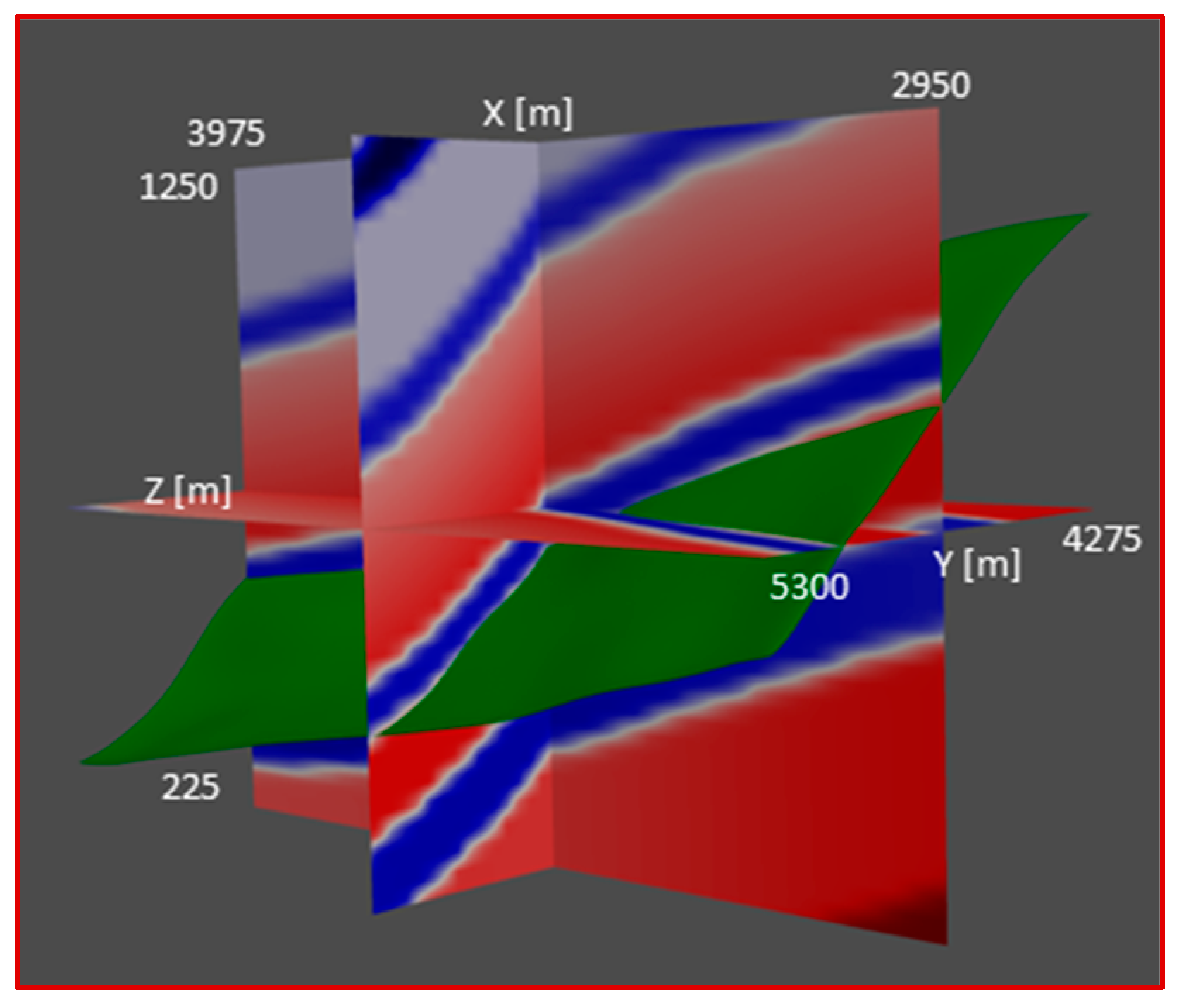
Following the well-log interpretation, the proposed horizon tracking method is used to fit a 3D horizon as the formation boundary for well 15-9-F-15D. The 3D location and shape of the fitted horizon, starting from the control points identified from the well logs, are compared with the depth-migrated 3D horizon interpretations in the field data in Figure 14. The fitted horizon and the horizon interpreted by the experts show good agreements over the majority of the volume with a depth difference less than 20 m, while most of the differences appear along the image edges.
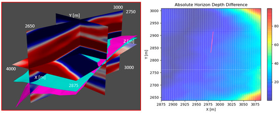
Figure 14.
Left: 3D horizon fitted through the boundary estimate (blue) plotted against 3D horizon from the Volve dataset (pink). Right: Heatmap of absolute depth difference between horizon in dataset and horizon fitting result. Both results are for well 15-9-F-15D.
There are a number of factors contributing to these differences between the seismic horizons and the fitted ones. First, the resolution of the seismic image is 12.5 12.5 4 m in the inline, crossline, and depth dimensions, respectively, which will inherently introduce the rounding error. Second, the geosteering team reported faults in this area that may not have been known to the human interpreters and is also not apparent in the seismic images used for this test. Furthermore, the crossline and inline slices of the seismic data in well 15-9-F-15D are plotted in Figure 15 and it illustrates that the least-squares horizon (the green line) closely tracks the event in the seismic image (boundary between light/dark color blocks). The interpretation produced by the geosteering team (the pink line) in the field is a comprehensive estimate combining multiple data sources and does not necessarily follow the event in the plotted seismic image. The comparison results between the final fitted horizon and the field interpretation in well 15-9-F-1C are plotted in Figure A2 and Figure A3 in the Appendix A.
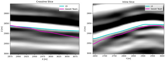
Figure 15.
Comparison of seismic horizons on crossline (left) and inline (right) slices of seismic image volume. Both results are for well 15-9-F-15D.
6. Conclusions
Bayesian well-log interpretation and horizon auto-tracking are each powerful tools for geological interpretation. This work presents the first framework that combines these tools into a fully automated geological interpretation workflow for geosteering optimization and automation. By interpreting 3D surface boundaries of the formation(s) of interest, the interpretation workflow removes the assumption of lateral continuity of the formation structure. Through the validation on the Overthrust and Volve datasets, the proposed algorithm illustrates the capabilities of accurate boundary estimation near the well path and precise representation of boundary shape changes further away from the well trajectory. The comparison between the geological interpretation reported by the geosteering team and that generated by the proposed algorithm indicates that human bias and interpretation uncertainty are minimized. These interpretations allow continual updates of the subsurface conditions while drilling and can either be used for more informed decision making by the directional driller or entered into a geosteering optimization workflow.
However, there are some limitations to the methods presented here. The log interpretation method requires careful preparation of a type log that correlates with the formation boundary, and robust, automated generation of such data is necessary future work. In addition, the seismic horizon tracking fits a surface to the seismic image and cannot identify features that are not present in the seismic data (e.g., faults not evident in the seismic image). Seismic images can also be noisy or ambiguous, so the horizon interpretation should be accompanied by an estimate of the uncertainty in the horizon depth. Lastly, since the particle filter is such a flexible interpretation tool, there is an opportunity to incorporate other information into the analysis that merits further exploration.
Author Contributions
Conceptualization, methodology, writing—original draft preparation, J.D.; methodology, validation, formal analysis, writing—original draft preparation, Z.Z.; validation, formal analysis, visualization, writing—review and editing, Y.Z.; validation, writing—review and editing, D.C.; writing—review and editing, project administration, P.A.; supervision, project administration, funding acquisition, E.v.O. All authors have read and agreed to the published version of the manuscript.
Funding
This research received no external funding.
Data Availability Statement
Publicly available datasets were analyzed in this study, which can be found here:. [Volve field dataset: https://data.equinor.com/, SEG/EAGE Salt and Overthrust Models: https://wiki.seg.org/wiki/SEG/EAGE_Salt_and_Overthrust_Models] (accessed on 10 February 2024).
Acknowledgments
The authors are grateful to the Rig Automation and Performance Improvement in Drilling (RAPID) program at the University of Texas at Austin and its sponsors for providing financial support for the development of this work. The authors would also like to acknowledge the use of the following open-source projects without which this work would not have been possible: Matplotlib, Numpy, Numba, OpendTect, Pyvista, and Scipy.
Conflicts of Interest
The authors declare no conflicts of interest.
Appendix A
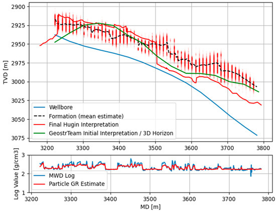
Figure A1.
Formation boundary estimation for well 15-9-F-1C.
Figure A1.
Formation boundary estimation for well 15-9-F-1C.
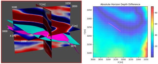
Figure A2.
(Left): 3D horizon fitted through the boundary estimate (blue) plotted against 3D horizon from the Volve dataset (pink). (Right): Heatmap of absolute depth difference between horizon in dataset and horizon fitting result. Both results are for well 15-9-F-1C.
Figure A2.
(Left): 3D horizon fitted through the boundary estimate (blue) plotted against 3D horizon from the Volve dataset (pink). (Right): Heatmap of absolute depth difference between horizon in dataset and horizon fitting result. Both results are for well 15-9-F-1C.

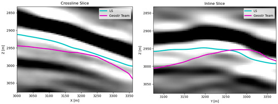
Figure A3.
Comparison of seismic horizons on crossline (left) and inline (right) slices of seismic image volume. Both results are for well 15-9-F-1C.
Figure A3.
Comparison of seismic horizons on crossline (left) and inline (right) slices of seismic image volume. Both results are for well 15-9-F-1C.
References
- Pehlivantu, C. Modeling, Guidance, and Control for Cost Conscious Directional Drilling. Doctoral Thesis, The University of Texas, Austin, Austin, TX, USA, 2018. [Google Scholar]
- Zheng, D. Path Optimization Advisory and Analytical Tools for Directional Drilling. Doctoral Thesis, The University of Texas, Austin, Austin, TX, USA, 2017. [Google Scholar]
- Kullawan, K.; Bratvold, R.B.; Bickel, J.E. Sequential geosteering decisions for optimization of real-time well placement. J. Pet Sci. Eng. 2018, 165, 90–104. [Google Scholar] [CrossRef]
- Alyaev, S.; Bratvold, R.B.; Luo, X.; Suter, E.; Vefring, E.H. An interactive decision support system for geosteering operations. In Proceedings of the SPE Norway Subsurface Conference, Bergen, Norway, 18 April 2018. [Google Scholar] [CrossRef]
- D’Angelo, J.; Khaled, M.S.; Ashok, P.; van Oort, E. Pareto optimal directional drilling advisory for improved real-time decision making. J. Pet Sci. Eng. 2022, 210, 110031. [Google Scholar] [CrossRef]
- Nguyen, K.L.; Fahmy, M.F.; Dzhaykiev, B.; Odiase, P.O.; Al-Morakhi, R.; Al-Ajmi, M.M.; Verma, N.K.; Quttainah, R. Application of Logging While Drilling-Nuclear Magnetic Resonance in Reservoir Evaluation and Geosteering: A Case Study in Marrat Reservoir, Umm Roos Field, West Kuwait. In ADIPEC; OnePetro: Richardson, TX, USA, 2022. [Google Scholar] [CrossRef]
- Kullawan, K.; Bratvold, R.; Bickel, J.E. A Decision Analytic Approach to Geosteering Operations. SPE Drill. Complet. 2014, 29, 36–46. [Google Scholar] [CrossRef]
- Griffiths, R. Well Placement Fundamentals; Schlumberger: Houston, TX, USA, 2009. [Google Scholar]
- Pyrcz, M.J.; Deutsch, C.V. Geostatistical Reservoir Modeling; Oxford University Press: Oxford, UK, 2014. [Google Scholar]
- Tearpock, D.J.; Bischke, R.E. Applied Subsurface Geological Mapping; Prentice Hall: Hoboken, NJ, USA, 1991. [Google Scholar]
- Feng, R.; Grana, D.; Balling, N. Variational inference in Bayesian neural network for well-log prediction. Geophysics 2021, 86, M91–M99. [Google Scholar] [CrossRef]
- Winkler, H. Geosteering by exact inference on a Bayesian network. Geophysics 2017, 82, D279–D291. [Google Scholar] [CrossRef]
- Miao, Y.; Kowal, D.R.; Panchal, N.; Vila, J.; Vannucci, M. Nonlinear state-space modeling approaches to real-time autonomous geosteering. J. Pet Sci. Eng. 2020, 189, 107025. [Google Scholar] [CrossRef]
- Chen, Y.; Lorentzen, R.J.; Vefring, E.H. Optimization of Well Trajectory Under Uncertainty for Proactive Geosteering. SPE J. 2014, 20, 368–383. [Google Scholar] [CrossRef]
- Luo, X.; Eliasson, P.; Alyaev, S.; Romdhane, A.; Suter, E.; Querendez, E.; Vefring, E. An ensemble-based framework for proactive geosteering. In SPWLA Annual Logging Symposium; SPWLA: Houston, TX, USA, 2015; p. SPWLA-2015. Available online: https://onepetro.org/SPWLAALS/proceedings/SPWLA15/All-SPWLA15/SPWLA-2015-KKKK/28497 (accessed on 27 November 2023).
- Jahani, N.; Garrido, J.A.; Alyaev, S.; Fossum, K.; Suter, E.; Torres-Verdín, C. Ensemble-based well-log interpretation and uncertainty quantification for well geosteering. Geophysics 2022, 87, IM57–IM66. [Google Scholar] [CrossRef]
- Veettil, D.R.A.; Clark, K. Bayesian Geosteering Using Sequential Monte Carlo Methods. Petrophys.-SPWLA J. Form. Eval. Reserv. Descr. 2020, 61, 99–111. [Google Scholar] [CrossRef]
- Muhammad, R.B.; Srivastava, A.; Alyaev, S.; Bratvold, R.B.; Tartakovsky, D.M. High-Precision Geosteering via Reinforcement Learning and Particle Filters. arXiv 2024, arXiv:2402.06377. [Google Scholar]
- Pakyuz-Charrier, E.; Giraud, J.; Ogarko, V.; Lindsay, M.; Jessell, M. Drillhole uncertainty propagation for three-dimensional geological modeling using Monte Carlo. Tectonophysics 2018, 747–748, 16–39. [Google Scholar] [CrossRef]
- Wu, M.; Miao, Y.; Panchal, N.; Kowal, D.R.; Vannucci, M.; Vila, J.; Liang, F. Stochastic clustering and pattern matching for real-time geosteering. Geophysics 2019, 84, ID13–ID24. [Google Scholar] [CrossRef]
- Albusairi, M.; Torres-Verdín, C. Fast-forward modeling of borehole nuclear magnetic resonance measurements acquired in deviated wells and spatially heterogeneous formations. Geophysics 2023, 88, D95–D113. [Google Scholar] [CrossRef]
- Wu, X.; Geng, Z.; Shi, Y.; Pham, N.; Fomel, S.; Caumon, G. Building realistic structure models to train convolutional neural networks for seismic structural interpretation. Geophysics 2020, 85, WA27–WA39. [Google Scholar] [CrossRef]
- Khan, M.M.; Alam, A. High Resolution Adaptively Steered Horizon Tracker. In International Geophysical Conference and Oil & Gas Exhibition, Istanbul, Turkey, 17–19 September 2012; SEG Global Meeting Abstracts; Society of Exploration Geophysicists and the Chamber of Geophysical Engineers of Turkey: Houston, TX, USA, 2012; pp. 1–4. [Google Scholar] [CrossRef]
- Geng, Z.; Wu, X.; Shi, Y.; Fomel, S. Deep learning for relative geologic time and seismic horizons. Geophysics 2020, 85, WA87–WA100. [Google Scholar] [CrossRef]
- Huang, L.; Dong, X.; Clee, T.E. A scalable deep learning platform for identifying geologic features from seismic attributes. Lead. Edge 2017, 36, 249–256. [Google Scholar] [CrossRef]
- Waldeland, A.U.; Jensen, A.C.; Gelius, L.-J.; Solberg, A.H.S. Convolutional neural networks for automated seismic interpretation. Lead. Edge 2018, 37, 529–537. [Google Scholar] [CrossRef]
- Alyaev, S.; Shahriari, M.; Pardo, D.; Omella, Á.J.; Larsen, D.S.; Jahani, N.; Suter, E. Modeling extra-deep electromagnetic logs using a deep neural network. Geophysics 2021, 86, E269–E281. [Google Scholar] [CrossRef]
- Fossum, K.; Alyaev, S.; Tveranger, J.; Elsheikh, A.H. Verification of a real-time ensemble-based method for updating earth model based on GAN. J. Comput. Sci. 2022, 65, 101876. [Google Scholar] [CrossRef]
- Alyaev, S.; Elsheikh, A.H. Direct Multi-Modal Inversion of Geophysical Logs Using Deep Learning. Earth Space Sci. 2022, 9, e2021EA002186. [Google Scholar] [CrossRef]
- Zhu, G.; Gao, M.; Wang, B. A robust inversion of logging-while-drilling responses based on deep neural network. Acta Geophys. 2023, 72, 129–139. [Google Scholar] [CrossRef]
- Thrun, S.; Burgard, W.; Fox, D. Probabilistic Robotics; Intelligent Robotics and Autonomous Agents Series; MIT Press: Cambridge, MA, USA, 2005. [Google Scholar]
- Wu, X.; Fomel, S. Least-squares horizons with local slopes and multigrid correlations. Geophysics 2018, 83, IM29–IM40. [Google Scholar] [CrossRef]
- Wu, X.; Hale, D. Automatically interpreting all faults, unconformities, and horizons from 3D seismic images. Interpretation 2016, 4, T227–T237. [Google Scholar] [CrossRef]
- Wu, X.; Janson, X. Directional structure tensors in estimating seismic structural and stratigraphic orientations. Geophys. J. Int. 2017, 210, 534–548. [Google Scholar] [CrossRef]
- Hale, D. Structure-oriented smoothing and semblance. CWP Rep. 2009, 635. Available online: https://inside.mines.edu/~dhale/papers/Hale09StructureOrientedSmoothingAndSemblance.pdf (accessed on 27 November 2023).
- Aminzadeh, F.; Brac, J.; Kunz, T. 3-D Salt and Overthrust Models: 3-D Overthrust Model Disk 1. 1; SEG/EAGE 3-D Modeling Series; Society of Exploration Geophysicists: Houston, TX, USA, 1997; Available online: https://books.google.com/books?id=oU-pQgAACAAJ (accessed on 10 February 2024).
- Equinor, Volve Field Dataset. Available online: https://data.equinor.com/ (accessed on 27 November 2023).


Disclaimer/Publisher’s Note: The statements, opinions and data contained in all publications are solely those of the individual author(s) and contributor(s) and not of MDPI and/or the editor(s). MDPI and/or the editor(s) disclaim responsibility for any injury to people or property resulting from any ideas, methods, instructions or products referred to in the content. |
© 2024 by the authors. Licensee MDPI, Basel, Switzerland. This article is an open access article distributed under the terms and conditions of the Creative Commons Attribution (CC BY) license (https://creativecommons.org/licenses/by/4.0/).