1. Introduction
Reducing greenhouse gas emissions is a key objective for many governments [
1,
2]. Also, Switzerland aims to achieve net-zero emissions by 2050, as set by the Federal Council [
3]. Achieving this target will require the introduction of new technologies to the energy market along with existing sources. Heating and cooling comprise half of the global energy consumption and over 40% of “energy-related CO
2 emissions”, surpassing electricity and transport [
4]. Underground Thermal Energy Storage (UTES) systems can address this by managing the seasonal mismatch between energy supply and demand, achieving energy savings of 40–70% and substantial CO
2 reductions, making them ideal for large-scale applications such as district heating and cooling [
5,
6]. UTES systems mainly include Aquifer Thermal Energy Storage (ATES), which stores heat and cold in aquifers for large-scale applications, Borehole Thermal Energy Storage (BTES), using closed-loop boreholes, as well as Tank (TTES) and Pit (PTES) Thermal Energy Storage, which store energy in tanks or pits, offering flexibility for smaller storage [
5]. Amongst these, ATES systems are particularly advantageous for large-scale applications due to their high storage capacity, enabling efficient seasonal heat and cold storage for extensive energy needs, such as in district heating and cooling grid networks [
6].
One of the earliest discoveries/applications of underground thermal energy storage (UTES) systems was in Shanghai, China, in the 1960s (when aiming for managing land subsidence), while similar experiments in 1974 in Neuchâtel, Switzerland, explored aquifer storage for seasonal heat management, both facing challenges with thermal dispersion, water chemistry changes, heat loss, and heat recovery efficiency [
7,
8,
9,
10]. Given that these issues were more manageable in low-temperature (LT-ATES) systems (below 40 °C), attention and development efforts shifted predominantly toward LT-ATES solutions [
5,
11,
12]. Today, the Netherlands leads in the deployment of LT-ATES systems with around 2500 installations, followed by Sweden with approximately 220 systems, whereas only about 1% of the ATES systems worldwide are HT-ATES [
5]. ATES systems are ideal for large-scale heating and cooling, such as in commercial buildings, district heating, and industrial facilities [
5]. In ATES, during summer, groundwater is extracted from the “cold well”, heated with available surplus energy, and then injected in the “warm well”, and in winter, the process reverses to retrieve the stored thermal energy from the warm well [
13]. In an ATES system, energy storage can be carried out using separate warm and cold boreholes (doublet system) at different depths or through a single borehole that injects and extracts both warm and cold water using separate lines and screens at different depths within the borehole [
14].
Despite the predominant use of shallow, low-temperature reservoirs, there is growing interest in exploring deeper storage options with higher temperatures. For example, as of 2023, Switzerland has lifted the previous restriction that limited heating of groundwater by more than 3 °C, specifically for deep groundwater not used for drinking, which facilitates the expanded use of geothermal energy and seasonal heat storage [
15]. For instance, the Forsthaus project in Bern, Switzerland, is a high-temperature heat storage project set to take place in sandstones at a depth of about 500 m [
16].
Several metrics exist for evaluating the performance of thermal storage systems. Among these, one widely examined parameter is heat recovery efficiency. This metric is typically defined as the ratio of the enthalpy extracted to the enthalpy injected over the course of an “injection–storage–extraction” cycle (the measure that is also used in the current study) [
17]. The efficiency of the thermal energy storage systems can be influenced, amongst many factors, by buoyancy flow, temperature differences between injected and ambient water, aquifer permeability/heterogeneity, storage cycle duration, distance between hot and cold wells, and well configuration design [
18,
19]. While conventional UTES systems, such as ATES and BTES, are well established for seasonal energy storage, Fractured Thermal Energy Storage (FTES), initially presented based on the idea of creating/utilizing hydraulic fractures in the borehole, presents an alternative approach with unique benefits and challenges [
20]. FTES offers a distinct approach to seasonal energy storage, combining the open-loop efficiency of ATES systems—requiring fewer boreholes for comparable storage capacity—with the broader applicability of BTES systems, as it does not rely on pre-existing permeable aquifers [
20,
21]. One of the earliest developments in FTES was the HYDROCK concept, which uses stimulated or artificially created fractures in shallow bedrock as conduits for hot or cold fluid, in which proppants can also be injected to maintain the aperture of the fractures [
21,
22]. As part of this project, field experiments in SW-Sweden’s Bohus Granite showed that this method could yield 10–20% more energy during extraction compared to traditional “ducted ground heat storages” [
21]. In another attempt, Ramstad et al. [
23] showed that hydraulic fracturing in crystalline bedrock, through water-only or sand-supported methods, increases thermal storage efficiency by creating extensive heat exchange surface area. Recent modeling studies, primarily based on simplified 2D [
24] or 3D [
20,
25,
26] (hydraulic) fracture geometries suggest that FTES could be a viable solution for thermal energy storage applications.
Despite promising results, to the author’s knowledge, to date, FTES has not been widely adopted nor explored. This can be attributed to the fact that FTES remains largely theoretical, and untested over a large scale and long term, and its performance can be significantly influenced by the existing natural fractures in the system, which can alter the dominant hydraulic flow pathway [
20,
21,
27,
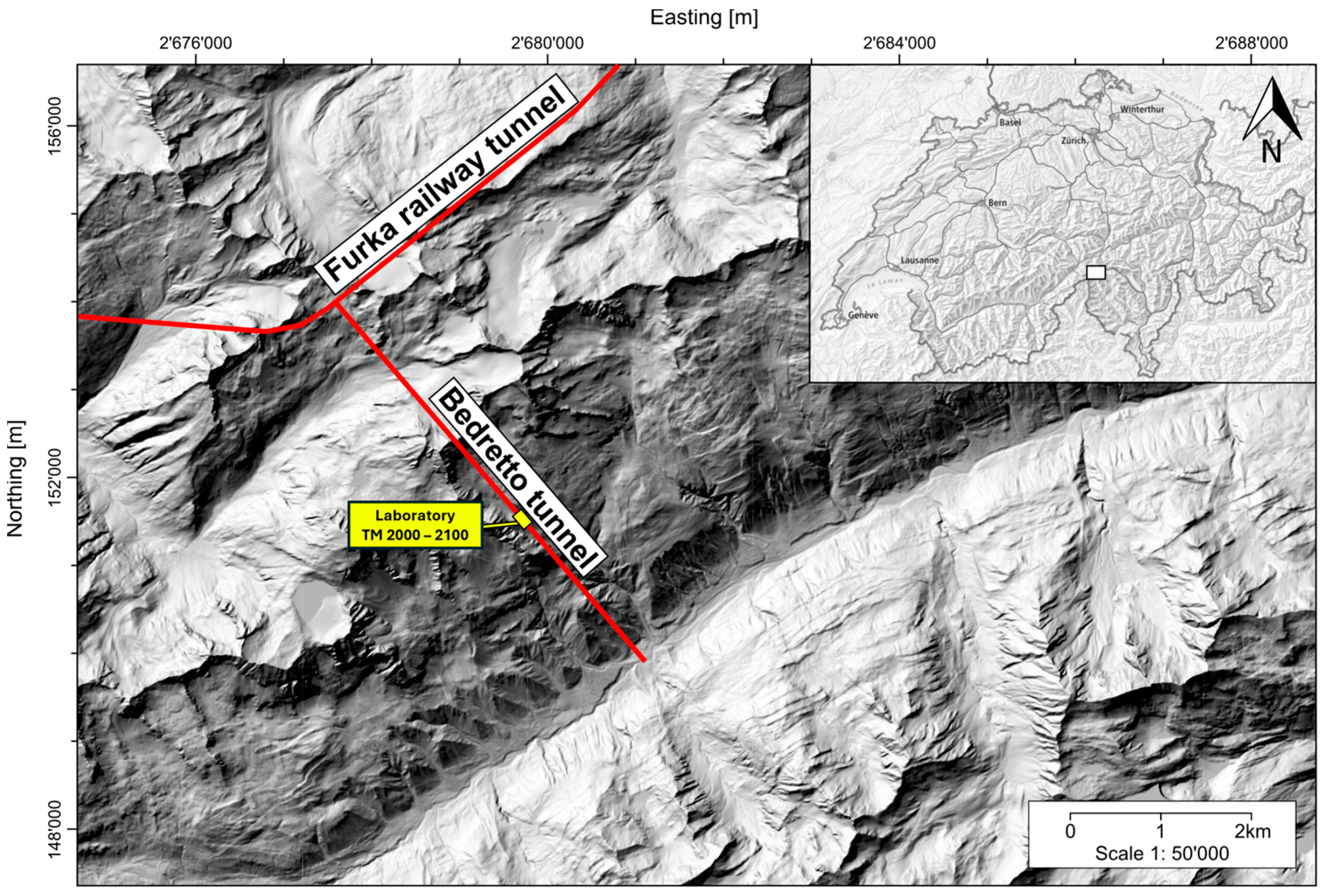
28]. This study aims to address some of these gaps by evaluating FTES performance in Switzerland’s Bedretto Underground Laboratory for Geosciences and Geoenergies (BULGG) [
29], utilizing its distinct geological features to assess the efficiency under realistic conditions. BULGG provides a unique opportunity to evaluate FTES systems’ potential in a controlled environment so that valuable insights can be obtained about the optimization of storage efficiency and its link to the complexities of the natural fracture systems. The objective is to determine energy efficiency using numerical modeling and to investigate the impact of different flow rates and injection temperatures on system efficiency. Additionally, the study will compare the efficiency of two well configurations: a single-well system and a doublet system. The studied energy storage cycles consist of four phases: injection, storage, production, and resting [
30] (corresponding to different seasons: injection in summer, storage in autumn, production in winter, and resting in spring). Moreover, the potential applications of extracted energy will be discussed.
3. Methodology
The COMSOL Multiphysics [
45] numerical solver is used to simulate fluid flow and heat transfer in the fractured reservoir domain intersected by the stimulation boreholes ST1 and ST2. COMSOL has been used in the past, for example, by Aliyu and Chen [
46], for modeling heat transfer and fluid flow in discretely fractured geothermal reservoirs, showing the effectiveness and robustness of such a numerical framework. In this study, a base case scenario was established to determine the energy efficiency of the storage system. In this study, one energy storage cycle comprises four phases, injection, storage, production, and resting [
30], each lasting 91 days to correspond with the four seasons of the year (a total of 364 days assumed annually, which is rounded for simplicity of simulation intervals). The injection phase takes place during the warmest months, from June to August, in this study. The production phase occurs from December to February, aligning with peak heat demand. This annual cycle repeats over a 25-year period, assuming the average operational lifetime of an ATES system [
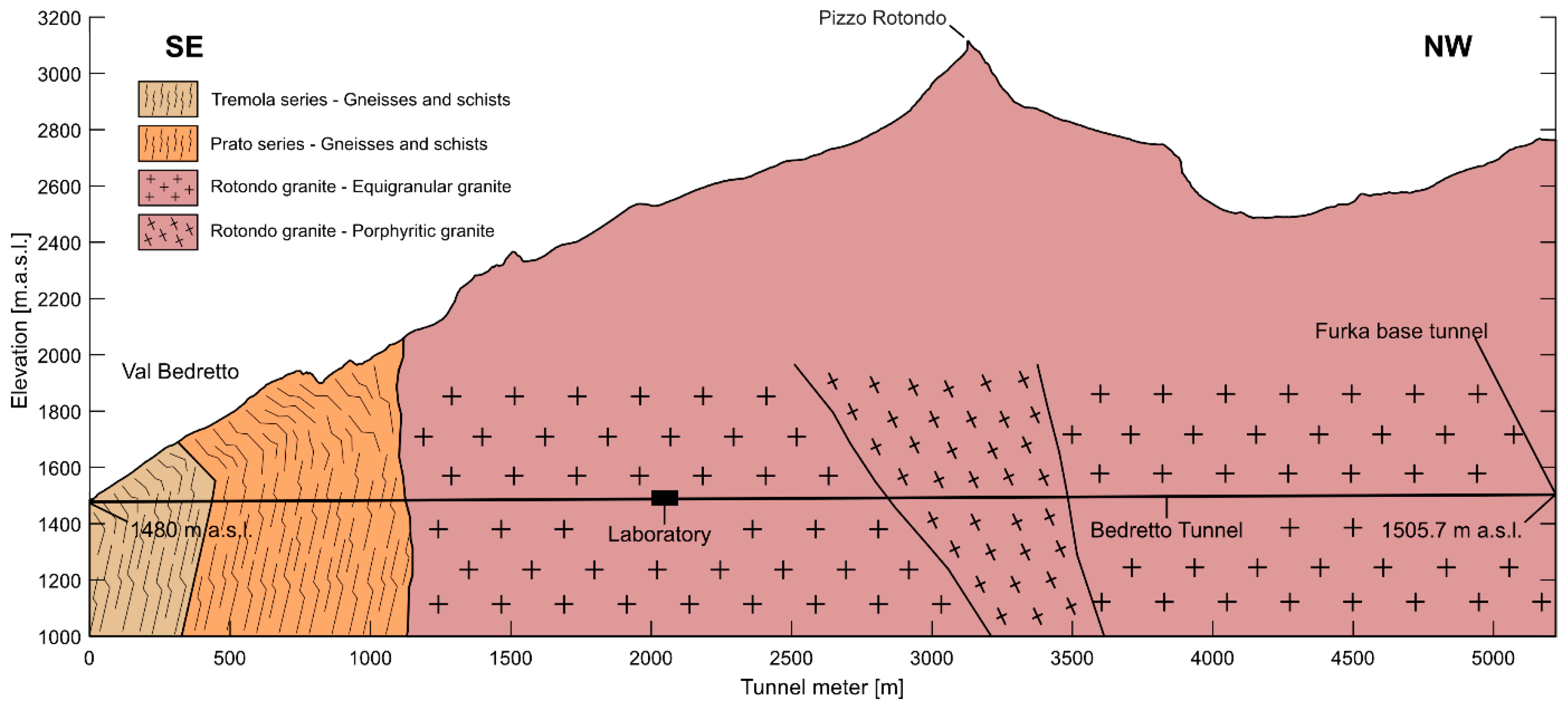
47]. Two well configurations were selected in highly transmissive structures crossed by the injection and production boreholes, ST1 and ST2: a doublet system and a single-well system. For the sake of clarity in describing the operational design, the terms “main interval” and “peripheral intervals” are introduced. The “main interval” refers to ST1-Interval 8, which is utilized for injecting hot water during the summer and producing hot water in the winter. The “peripheral intervals” refers to ST2 intervals in the doublet system configuration or ST1-Interval 9 in the single-well system, which are used for cold water operations. The most transmissive fault zone intersected by the upper part of ST1 is found in zonally-packed Interval 8 [
43] and is used in this case study as the main well for injecting hot fluid in summer and producing hot fluid in winter. Interval 8 extends between measured depths 186.7 m and 216.8 m in ST1, crossing the major permeable fault zone at 208.2 m [
43,
44]. Previous experiments have shown that water injected into Interval 8 of ST1 reaches Interval 9 in the same well, as well as the ST2 borehole, likely at depths of 211.8 m and 285.7 m [
43]. Therefore, in the case of a single-well setup, Interval 9 is considered as the peripheral interval in ST1, which extends between measured depths of 170.8 m and 185.2 m, crossing two major permeable fault zones at measured depths of 174.1 m and 183.2 m. In the case of the doublet well system, the two permeable zones of ST2 (peripheral intervals) are found at measured depths of 211.8 m and 285.7 m. It is important to note that while other fractures in the abovementioned intervals may also contribute to fluid flow, quantifying their specific contributions remains challenging. Therefore, the measured interval transmissivity is attributed only to the selected fault zones. The doublet system involves injecting hot water in summer into ST1 in Interval 8 and producing cold water from two distinct peripheral zones in ST2 and vice versa in winter. The single-well system operates within ST1 by injecting hot fluid into Interval 8 and producing cold fluid from Interval 9 in the same borehole. Injection temperatures were set at 60 °C, typically the maximum achievable by a heat pump in case of using such technology with tunnel water as the heat source, and 120 °C to explore the potential for electricity production. To maintain the hydraulic gradient between the main well and the peripheral well, simultaneous water injection and production is performed throughout the operational phases.
During the summer, hot water is injected into the ST1, while the production intervals are exposed to atmospheric conditions within the tunnel. The produced fluid is then utilized for re-injection into ST1-Interval 8 after being heated to the predefined injection temperature. If the flow rate of the produced fluid from the peripheral interval is lower than the injection rate at ST1-Interval 8, the difference is compensated by water from the tunnel. This water, collected by fault outcrops along the tunnel wall, supplements the periods of insufficient flow from peripheral wells to maintain the predefined injection flow rate. In the winter production phase, water is injected either into ST2 in a doublet system or into ST1-Interval 9 in a single-well system, utilizing tunnel water that maintains a temperature of ca. 16.8 °C [
32]. During this period, the mass of water produced is the same as that of the water injected.
To assess the influence of the injection rates on heat recovery efficiency, three injection rates were selected for both the single-well and doublet systems: 1 kg/s, 1.5 kg/s, and 2 kg/s. For the sake of simplicity, unless otherwise stated, the term ’flow rate’ in this study refers to the mass flow rate. These rates were chosen based on previous experiments at Bedretto Lab. and the estimated minimum principal stress magnitude in the reservoir [
48], making sure that they are unlikely to induce hydraulic fracturing in the reservoir volume. For better numerical stability, the imposed flow rates in the numerical model are ramped linearly from zero over the first day of each injection and production phases. In addition to determining the recovery efficiency of the energy storage system, other analyses using the produced water were also conducted, including transportation to a hypothetical usage site and an evaluation of the potential for electricity production.
3.1. Reservoir and Fracture Setup
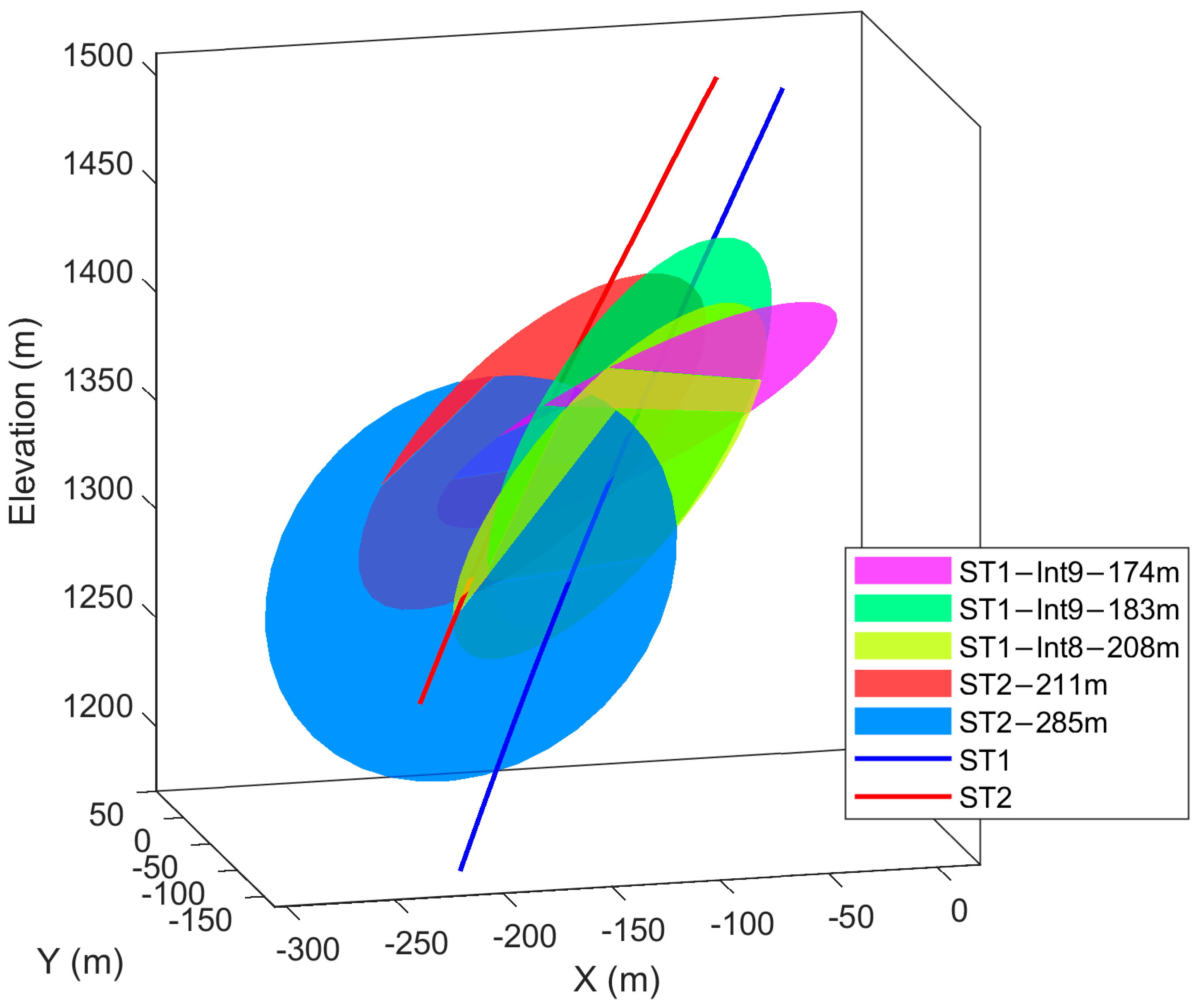
The reservoir model used in this study is shown in
Figure 3. As shown in the figure, this model includes the two boreholes, ST1 in blue and ST2 in red, intersected by various major faults/fractures assumed and represented as planar structures with a radius of 100 m. The reservoir is represented by a 325 m × 220 m × 340 m granitic domain. The structure of the tunnel, located at the top of the wells, was excluded from the numerical model.
The measured properties of the faults and fractures, including transmissivity values, are presented in
Table 1. Given the initially low transmissivity of some of the faults and to further reduce the pumping power requirement during the injection and production, stimulation operations are assumed to be conducted both near the wellbore and at a large scale. This is assumed to increase the transmissivity of all faults by an order of magnitude over large-scale and to introduce a skin factor of −2 in the near-wellbore region of the peripheral wells. As a result, the maximum large-scale transmissivity of the faults in the reservoir volume reaches 1.1 × 10
−5 m
2/s—a level previously observed in the deeper intervals of ST1 within the Bedretto reservoir volume [
41].
Water properties—such as dynamic viscosity, thermal conductivity, specific heat capacity, and density—are calculated based on the COOLPROP library [
52], which provides these properties as functions of pressure and temperature. The properties of granite rock matrix, including thermal conductivity and specific heat capacity, are set based on COMSOL’s built-in material library [
45], specifically using the data for fine-grain granite. For the fault material, the properties are assumed to be 1200 kg/m
3 for density, 3 W/(m × K) for thermal conductivity, and 790 J/(kg × K) for specific heat capacity. The connected and total porosity of the granite is set to 1.36% and 1.75%, respectively [
53]. Fracture porosity is assumed to be 10%. The specific storage of the faults/fractures (
Ss) is assumed as 10
–6 m
–1 [
54].
The initial temperature of the model was set according to the temperature values recorded on 18 October 2024, by the installed fiber optics in ST1 using an XT-DTS temperature interrogator (with a resolution of 0.01 °C) [
55], ranging from ca. 18 °C at the top of ST1 (wellhead) to ca. 26 °C at the bottom of the borehole. The fiber optic measurement was calibrated with an RBR Solo T probe with an accuracy of 0.002 °C [
56], co-located with a section of the fiber in an insulated bath. The granitic rock domain was extended vertically in the numerical model to include the upper part of the tunnel. A constant temperature, equal to the temperature at the top of the ST1 borehole, was applied from the top of the model to the wellhead. The temperature values were linearly extrapolated below the ST1 wellhead. A linearly extrapolated pressure gradient was also applied using recorded pressure values in ST1 packed intervals, from wellhead to the bottom of the model, including the assumption of atmospheric pressure at the wellhead. The pressure from the top of the model to the ST1 wellhead is assumed constant as the initial condition. The boundary conditions for the model were defined such that the outer boundaries were assigned the initial pressure values, and open boundary conditions were applied for heat transfer over the model boundaries.
3.2. Energy Efficiency Estimation
The recovery efficiency of the energy storage system is calculated using Equation (1) below [
17]:
where
Φ represents the energy efficiency, and
EExt and
EInj are the extracted and injected enthalpies, respectively, estimated using the COOLPROP library [
52].
3.3. Water Flow in Pipes
The hot water extracted from the main well in winter is assumed to be transported to its end-user location through insulated pipes. Properties of pipes from companies like Jansen—for example, the model JANSEN bianco [
57]—were selected for the quantitative analysis of the system. These pipes are made of polyethylene and insulated with a layer of polyurethane (PU) foam, which has a thermal conductivity of 0.03 W/(m × K) [
57]. The chosen pipe has a diameter of 11 cm and an insulation thickness of 2.5 cm, a typical standard configuration that balances effective insulation with manageable heat loss. The pipes are assumed to be buried under the surface. The temperature loss along the pipe can be calculated using Equation (2) [
58]:
where
Te(
L) is the temperature (K) of the fluid passing through the pipe at a distance
L (m) from the source,
Tt is the outside air temperature (K),
Te0 is the initial temperature of the fluid (K),
K is the heat transfer coefficient of the pipe (W/(m × K)),
L is the pipe length (m),
Qwater is the water mass flow rate (kg/s), and
Cp,w is the specific heat capacity of the water (J/(kg × K) [
32,
58]. The temperature inside the tunnel, used in Equation (2), is determined based on measurements from the existing fiber optic line installed along the tunnel (measured using the XT-DTS temperature interrogator with a resolution of 0.01 °C [
55] and calibrated with RBR Solo T probe [
56]), which continuously records tunnel temperature. The external temperatures of 16.63 °C and −4 °C [
59] have been used as the average winter temperatures (corresponding to the production period) for the tunnel interior (from installed fiber optics) and the external atmospheric conditions, respectively. These values represent the average typical temperature in the time interval between December and February. Two potential sites for utilizing the hot water are proposed: the village of Bedretto, located 1.6 km from the southern portal of the tunnel, and a hypothetical greenhouse farm situated 200 m from the tunnel portal.
3.4. Thermal Energy and Power Management for Injection Scenarios
It is assumed that a photovoltaic solar panel installation outside the tunnel powers the heat pump or boiler for water heating, and the water pump, both of which utilize tunnel water. An electrical boiler or a water-to-water heat pump will be required to increase the injection water temperature, which is sourced from the water flowing out of the peripheral intervals as well as from the water flowing in the tunnel, from a minimum of 16.8 °C to 60/120 °C (depending on the system setup). Halter et al. [
32] showed that the capacity of total extractable thermal power from Bedretto tunnel water, when using a heat pump to cool tunnel water down to 4 °C, is between 0.8 MWth and 1.5 MWth. For the 120 °C injection scenario, an electrical boiler is necessary to heat the water, in particular from 60 °C to 120 °C. In total, for the most conservative case, when using both heat pump and electric boiler, with the assumption of a coefficient of performance of 3 for the heat pump [
60] and a typical efficiency of 90% for the boiler [
61], a total electrical power of approximately 0.7 MW will be required to increase the water temperature from 16.8 °C to 120 °C at the maximum flow rate of 2 kg/s. However, the produced fluid from the peripheral well is always above the tunnel water temperature that will be used for re-injection and therefore reduces heating power requirement estimates. To ensure a continuous supply of hot water during both the day and night in the summer, part of the electricity generated by the photovoltaic solar panel during the day needs to be stored in batteries. During the winter hot production phase—specifically for a 120 °C injection scenario—the feasibility of employing an Organic Rankine Cycle (ORC) engine with a typical net efficiency between 3% to 5% using, for example, the refrigerant HFC-134a as working fluid [
62,
63] for electricity generation will be investigated. The temperature of the water after passing through the ORC is assumed to be decreased to 30 °C. As part of this assessment, the potential for electricity generation is determined by comparing the average power output from the ORC during the winter to the power required for pumping.
The energy required by the water pumps can be estimated using Equation (3) [
64] as follows:
where
r is the pumping rate (m
3/h),
ρw is the density of the water (kg/m
3),
g is the gravitational acceleration (m/s
2),
h is the pressure head (m), and
η is the overall pump efficiency, chosen to be 60% int his study [
64]. The power
P in this formula is expressed in kW
e.
3.5. Numerical Modeling of Fluid Flow and Heat Transfer
In this study, the mass and energy balance in fractured porous media are solved using COMSOL Multiphysics numerical solver [
45]. The mass balance in the porous medium is described by Equation (4) as follows [
45,
65]:
where
ϵp represents the porosity of the medium (assumed to be constant in this study and therefore, is factored out of the differential equation),
ρw is the density of water,
u is the Darcy velocity, and
Qm represents mass sources or sinks. The Darcy velocity,
u, is calculated based on Darcy’s law as follows [
66]:
where
k is the permeability of the medium,
μ is the dynamic viscosity of the fluid, ∇
p is the pressure gradient, and
g is the acceleration due to gravity. The permeability is calculated based on transmissivity (listed in
Table 1) [
66].
The energy balance in the porous media is governed by Equation (6) [
45,
65]:
where (
ρCp)
eff represents the effective heat capacity of the medium,
Cp,w is the specific heat capacity of water, ∇
T is the temperature gradient,
q is the heat flux,
Q is the volumetric heat sources or sinks. The heat flux
q is computed as follows with Equation (7) [
45,
65]:
where
keff is the effective thermal conductivity of the medium.
The same mathematical procedure used for the porous medium is applied to fractures, which are represented in the model as 2D geometries with zero thickness. This approach simplifies the mesh design and enhances computational efficiency by mathematically incorporating the fracture apertures into the numerical equations without any physical thickness within the mesh [
67,
68,
69].
The numerical model built in COMSOL was validated against the analytical approach of Cheng et al. [
70] for a simplified 3D model configuration intersected by a planar fracture, employing typical reservoir parameters as outlined by Zinsalo et al. [
71]. A strong agreement was observed between the numerical results and the analytical solution, confirming the accuracy of the model. The detailed validation model and the obtained results are presented in
Supplementary Materials.
For the case studies considered in this investigation for FTES, an implicit solver using the Backward Differentiation Formula (BDF) method with adaptive time-stepping (the default setting in COMSOL for the developed time-dependent model) and a maximum allowed time step of 30 days, was employed to solve the heat transfer and fluid flow in the reservoir domain [
45]. The default Algebraic Multigrid (AMG) solver was used to solve the pressure and temperature variables [
45].
3.6. Meshing and Sensitivity Analysis for Optimal Size Selection
For simulating fluid flow and heat transfer, tetrahedral and triangular elements are used within the rock matrix and fractures, respectively. An analysis was performed to find an optimal balance between the number of degrees of freedom based on the selected mesh size, and the computational stability. The single-well case with a flow rate of 2 kg/s and injection temperature of 120 °C was selected for this analysis. Additionally, the impact of relative tolerance and maximum timestep size of the numerical solver are evaluated.
3.7. Assumptions in the Numerical Model
The presented model assumes an isotropic medium for the rock matrix and fracture. The model solves fluid dynamics and thermal behavior without incorporating rock deformation. The model also assumes no background natural groundwater flow. The heat loss through the borehole walls is not considered. The compressibility values for the faults/fractures are assumed to be constant. Although several natural fractures are observed in different intervals, only the major flow zones with demonstrated flow signatures are considered in the model. The transmissivity of the two permeable fault zones within Interval 9 of ST1 is assumed to be equal. The designated flow rate in Interval 9 in the ST1 wellbore is equally distributed between the two faults within this interval, assuming the necessary well completion is in place. Similarly, for the ST2 wellbore, the two flow zones located at 211.8 m and 285.7 m are assumed to equally share the designated flow rate. The influence of the subsurface heat flux from the bottom of the model was assumed to be negligible, given the timescale of the current study.
4. Results
4.1. Effect of Mesh Size, Relative Tolerance, and Time Stepping
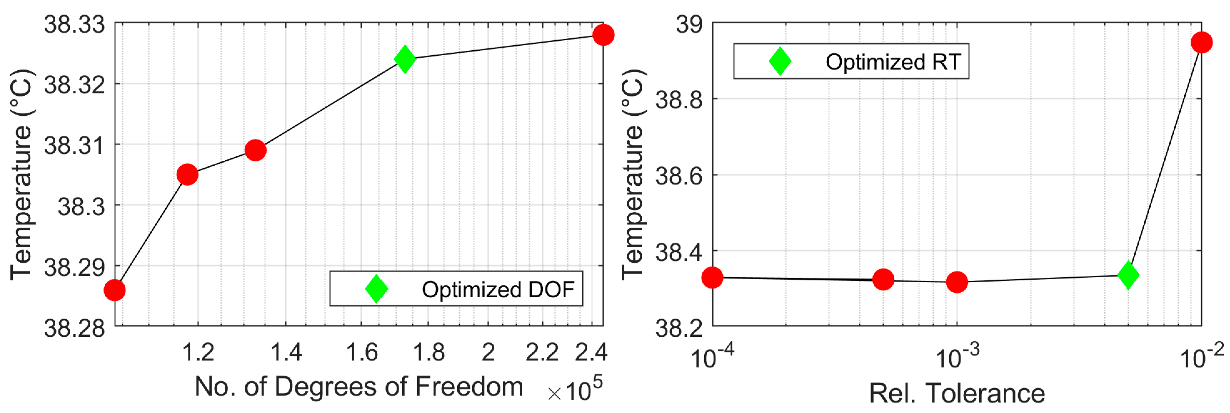
Figure 4 illustrates the impact of mesh size (left) and relative tolerance of the numerical solver (right) on the stability of the numerical results. The results are presented in terms of stability of the temperature at the main well at the end of one cycle for the case of single-well with a flow rate of 2 kg/s and injection temperature of 120 °C.
Mesh sizes for different faults/fractures were varied selectively using predefined settings in COMSOL Multiphysics, ranging from ‘coarse’ to ‘extra-fine’ [
45]. A relative tolerance of 5 × 10
−4 was selected for the mesh size analysis. A reasonable balance between mesh size and computational time, indicated by the green diamond in
Figure 4 (left), was selected for our simulations. The final optimized mesh used for the case studies in this research consists of 514,837 tetrahedral elements representing the rock matrix and 32,010 triangular elements representing the fault planes. The minimum size of the triangular elements within the fault plane mesh is ca. 0.4 m.
Furthermore, the influence of the relative tolerance of the numerical solver on the stability of the results is assessed by varying the tolerance between 10
−4 and 10
−2, using the optimized mesh configuration obtained from the previous step. The findings, displayed in
Figure 4 (right), indicate that a relative tolerance of 5 × 10
−3 provides an optimal computational efficiency, and therefore, this tolerance was subsequently used for the remainder of the study.
In addition, to verify the temporal accuracy of our model, a time-stepping comparison was conducted using the optimized mesh and relative tolerance. The default COMSOL time-stepping algorithm (as mentioned in
Section 3.5) with the maximum allowed time step of 30 days (with interpolated daily output results) was compared against a model configured with a maximum allowed time step of one day. This analysis showed very small temperature difference at the injection point, with differences of less than 0.01 °C after one full cycle, confirming the stability of the simulation results.
4.2. Heat Storage Model
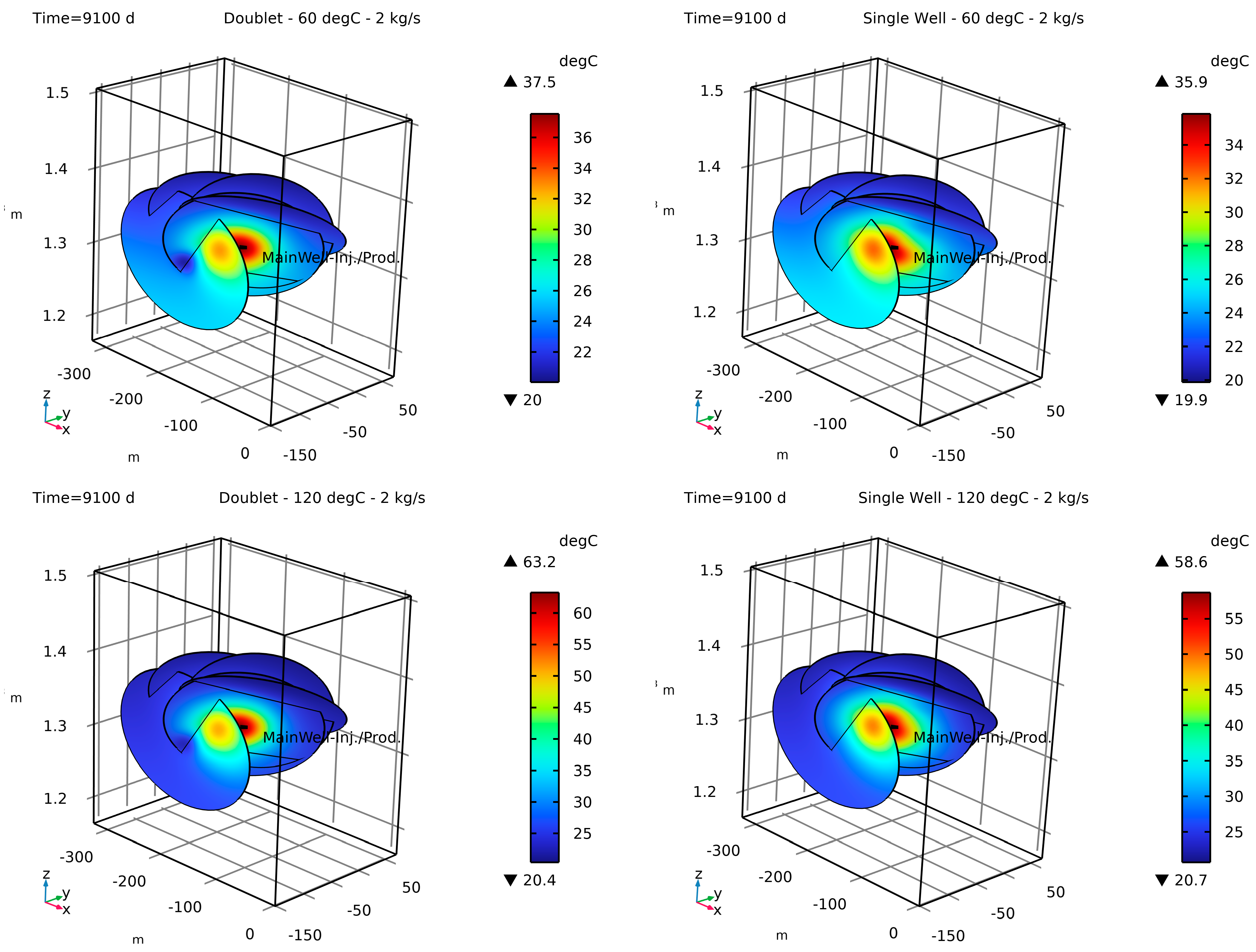
As an example, the numerical results of the heat storage model are shown in
Figure 5, illustrating the temperature distribution over the faults’ surfaces at the end of the 25th storage cycle, corresponding to an injection rate of 2 kg/s at temperatures of 60 °C (top) and 120 °C (bottom), and different well configurations, namely doublet (left) and single-well (right). Also shown in each figure is the location of the main well (Interval 8 in ST1). The numerical results reveal that the maximum temperature over the fault surface is consistently higher in the doublet system compared to the single-well setup. For instance, at an injection temperature of 60 °C, the temperature difference is approximately 1.6 °C, which increases to around 4.6 °C at 120 °C. This can be attributed to a more uniform thermal front propagation around the main interval in the doublet system, which enhances the heat distribution over the fault surfaces. In contrast, the single-well system, particularly near the peripheral intervals, shows a less uniform thermal front pattern. Additionally, while the dominant flow paths in the single-well setup include structures intersecting the main well (ST1), the faults intersecting the ST2 well also show thermal anomalies even in a single-well setup. This is particularly noticeable for the structure in ST2 at a depth of 211.8 m, where its intersection pattern with fractures intersecting with ST1 is more extensive (in terms of intersection length), therefore increasing the observed anomaly.
4.3. Transient Temperature Profiles Evolution in Injection/Production Wells
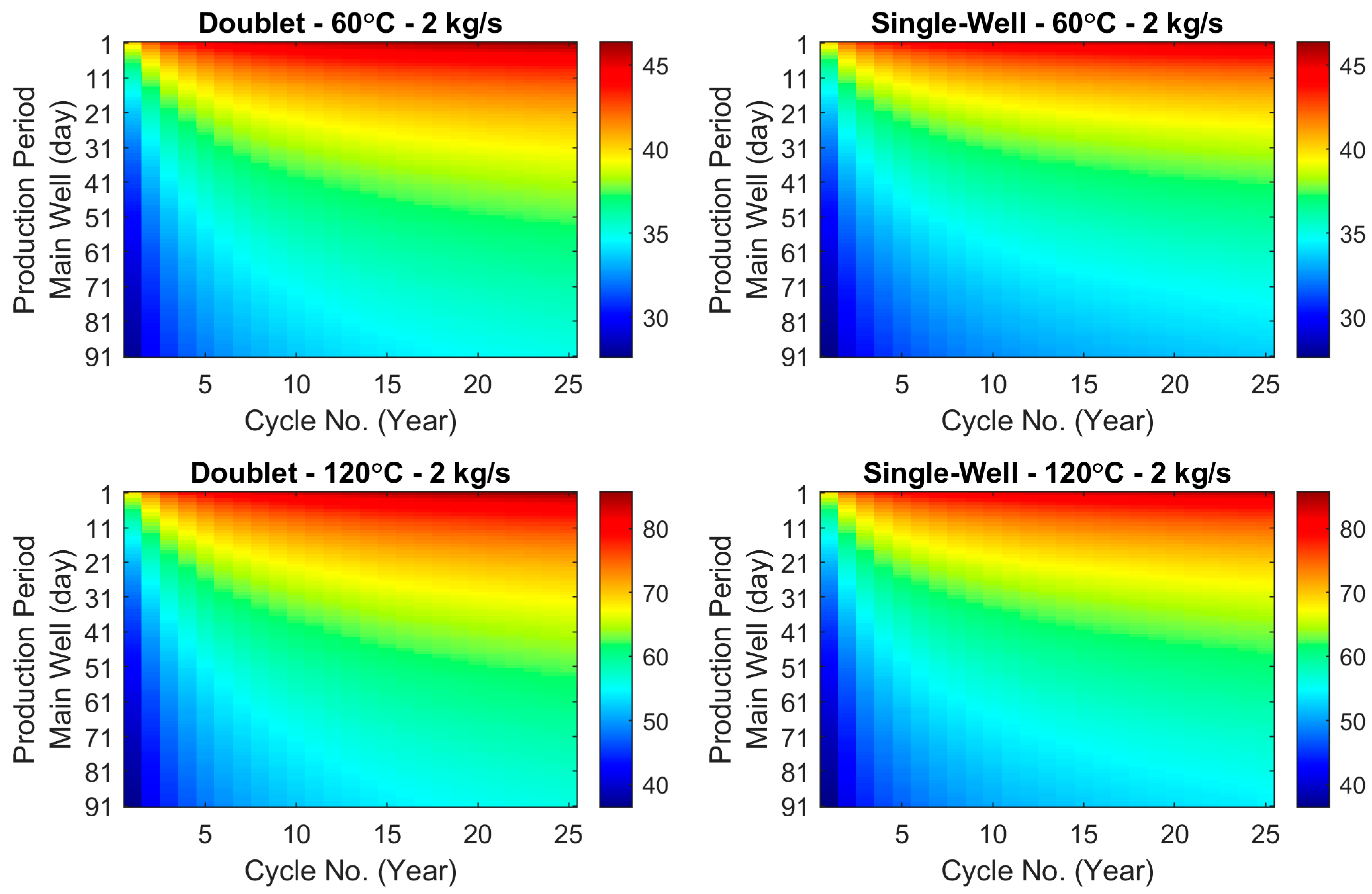
To better understand the transient temperature evolution between main and peripheral wells during the injection and production phases, the temperature profiles of the produced fluid from the peripheral intervals are analyzed for different cases in this study. These cases include different well setups (doublet- and single-well) and injection temperatures (60 °C and 120 °C) for the largest modeled injection flow rate (2 kg/s). The temperature profiles over both injection (summer) and production (winter) periods across all 25 cycles are presented in
Figure 6 and
Figure 7, respectively. As shown in
Figure 6, each subsequent injection period begins with the production of colder fluid from the peripheral interval. This is a result of the cold fluid injection in the peripheral interval during the preceding production phase. The single-well setup generally shows a faster increase in the temperature of the produced fluid, most likely due to the shorter distance between the main and peripheral intervals.
However, in both the single-well and doublet setups, particularly during the initial injection period, the start of thermal breakthrough in the peripheral interval due to hot water injection in the main well at 120 °C case happens more rapidly compared with the 60 °C scenarios. Specifically, in the doublet system, an anomaly—manually defined as at least a 0.2% change in the temperature of the produced fluid with respect to the initial in situ temperature—happens approximately 12 days earlier, at about day 32. In the single-well setup, the same anomaly threshold is reached about six days earlier than in the lower-temperature cases. Additionally, the results indicate that increasing the injection temperature from 60 °C to 120 °C in the main well results in an increase in the observed maximum temperature at the peripheral interval by the 25th cycle, with a rise of approximately 11 °C for the doublet setup and 10.4 °C for the single-well setup.
The results for the produced fluid temperature from the main well during the production period (winter), as shown in
Figure 7, indicate that the maximum produced temperature from the main well reaches approximately 46 °C for the 60 °C injection case and about 86 °C for the 120 °C injection case.
4.4. Energy Efficiency Pattern
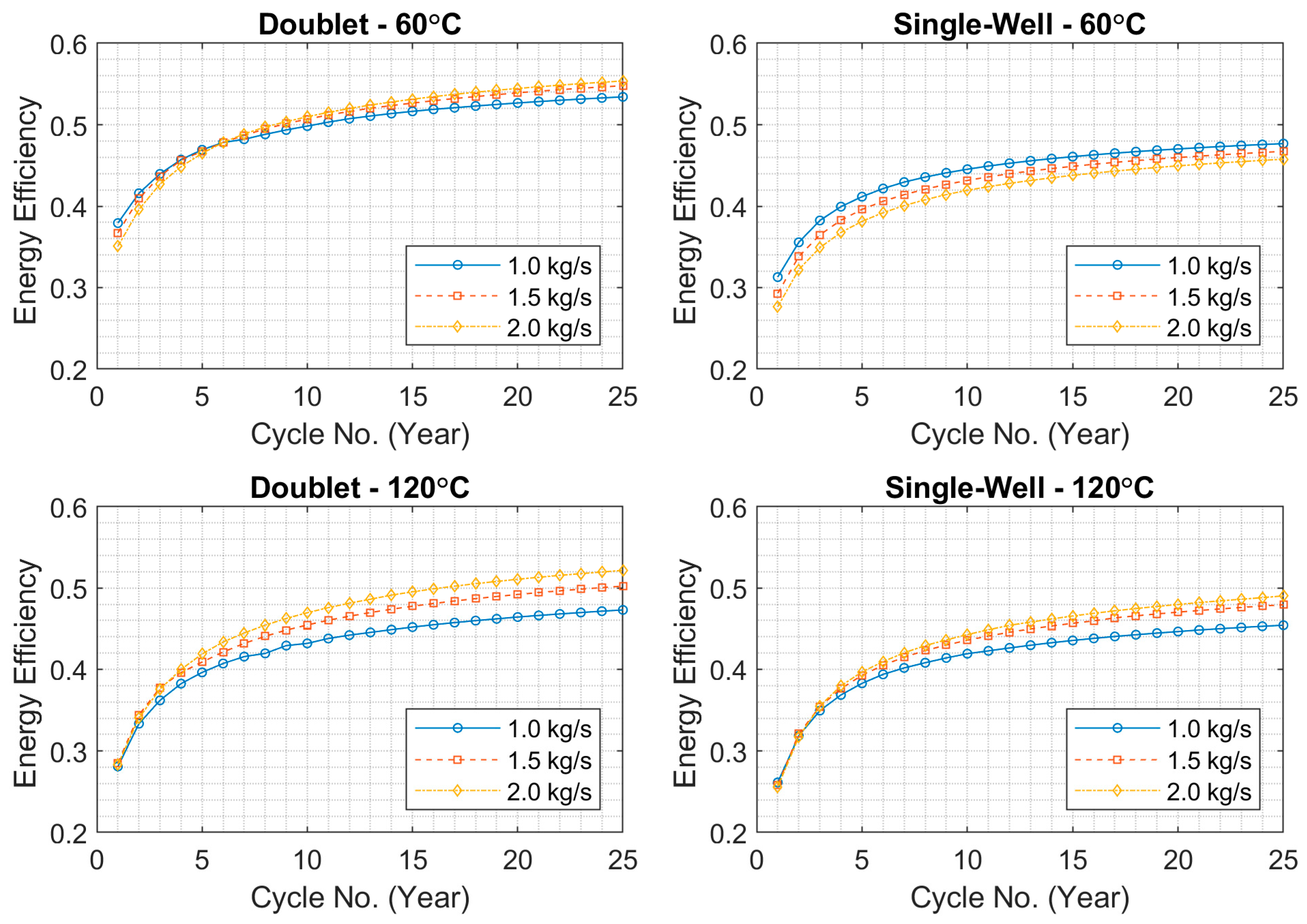
The energy efficiency for each injection rate and temperature was calculated for both the single-well and doublet systems over 25 cycles according to Equation (1), and the results are presented in
Figure 8. The results show that efficiency generally increases over time, and except for the case of the single-well at an injection temperature of 60 °C, higher flow rates generally yield higher energy efficiency by a maximum increase of ca. 10% for the doublet system at 120 °C when increasing the flow rate from 1 kg/s to 2 kg/s. Additionally, in the single-well setup at 60 °C, efficiency consistently decreases with increasing flow rate; however, the differences between flow rate cases decrease as the number of annual cycles increases. In the single-well system at 120 °C, efficiency increases notably by a maximum of ca. 6% after 25 cycles when the flow rate is raised from 1 kg/s to 1.5 kg/s. However, there is a minor increase in efficiency when the flow rate is increased from 1.5 kg/s to 2 kg/s.
In general, the doublet achieves higher efficiency in the investigated cases than the single-well setup. For example, for the 1 kg/s injection scenarios, the doublet system achieved ca. 12% and 4% higher efficiencies than the single-well system for the 60 °C and 120 °C cases, respectively. While in the single-well setup, increasing the injection temperature from 60 °C to 120 °C had a relatively lower impact on overall efficiency after 25 annual cycles, the doublet system showed a lower efficiency for the 120 °C case by the end of the 25 cycles compared with the 60 °C. It is also observed that, in the doublet setup at 60 °C, lower flow rates yielded higher efficiency at the early cycles compared to higher flow rates, specifically during the first five cycles. Also, in both single-well and doublet systems, for the 120 °C case, the efficiencies are nearly identical across different flow rates during the first two annual cycles. In contrast, for the 60 °C case, the efficiencies differ from the beginning across the studied flow rates. The results indicate that the doublet system using an injection temperature of 60 °C and an injection flow rate of 2 kg/s is the most efficient among all the case studies examined.
4.5. Water Flow and Temperature Loss
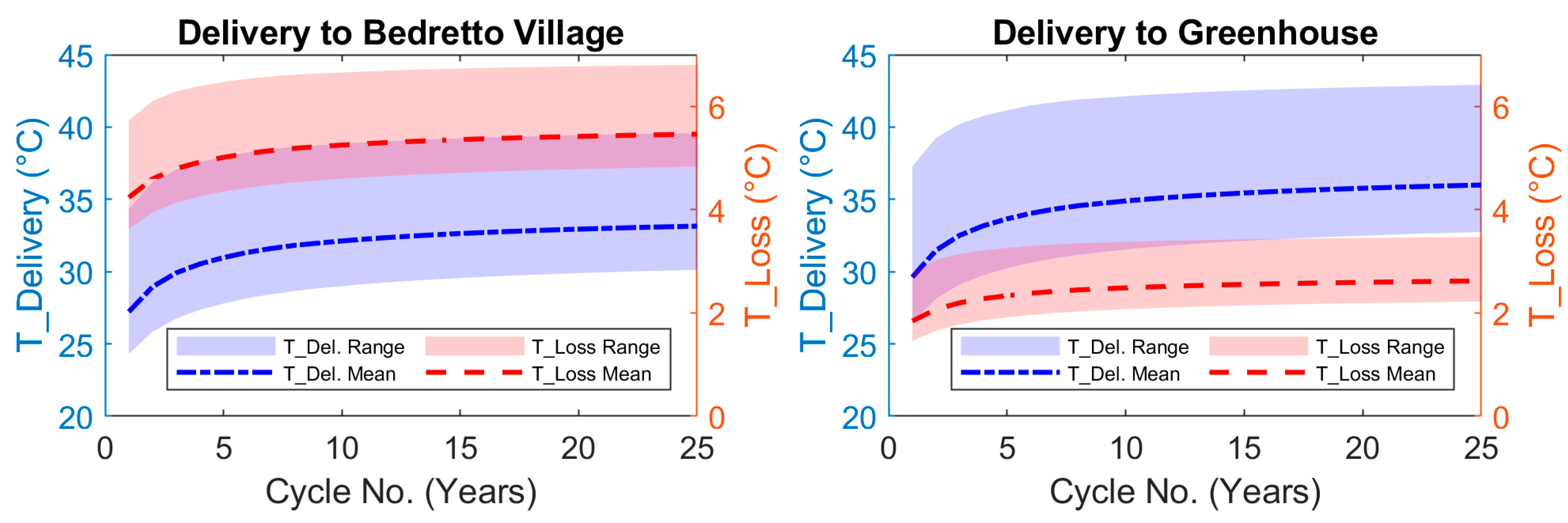
Figure 9 illustrates the delivered temperature of the hot produced water and its loss during the transport from the production well at TM 2000 to the village of Bedretto considering 3600 m of piping distance (left), as well as to the hypothetical greenhouse farm assuming 2200 m of piping distance (right). The best scenario with a maximum achieved efficiency was chosen for both cases, namely the 60 °C scenario with the doublet system with an injection rate of 2 kg/s, as mentioned in
Section 4.4. The temperature at the end destination and the temperature loss are calculated using Equation (2). The colored zones in
Figure 9 correspond to the minimum and maximum values for both temperature and temperature loss for each complete cycle.
The minimum temperature of the water arriving at the village of Bedretto is 24.3 °C during the first cycle, increasing to a minimum of 30.1 °C after 25 cycles (
Figure 9 left). The maximum temperature reaching the village ranges from 34.3 °C in the first cycle to 39.6 °C in the last cycle. For the hypothetical greenhouse farm located 200 m from the tunnel portal (
Figure 9 right), the minimum temperature of the arriving water is 26.5 °C during the first cycle and 32.7 °C during the last cycle. The maximum temperature reaching the greenhouse farm varies between 37.3 °C and 42.9 °C over the observed period. During the first cycle, the mean temperature loss at the village entrance is 2.4 °C higher than at the greenhouse case. This difference gradually increases to 2.8 °C by the 25th cycle.
4.6. Techno-Economic Analysis
During the 25-cycle evaluation period, a typical ORC can yield an average produced power of ca. 10.6 kW in winter, with peaks reaching 18.1 kW and dropping to a minimum of 2.3 kW. This contrasts with just the estimated average pumping power requirement of 21.1 kW for the same period, excluding heat storage, operational costs and initial investments.
For the heating case study, particularly for the most efficient case, i.e., the doublet system with injection temperature of 60 °C at 2 kg/s, we evaluated the techno-economic and environmental performance of the proposed FTES system, assumed to be powered solely by solar-PV-based system and using electrical boiler for heating of the water, including information from economic and environmental factors, such as carbon intensity and the cost of avoided carbon emissions.
The carbon intensity of the whole system is dominated by the emissions from site preparations/drilling/completion of boreholes, surface piping installations, and the solar PV system, which are assumed for our analysis based on typical values presented by McCay et al. [
72], as 2.82 tCO
2/m, 248.75 kg CO
2/m, and 46 kg CO
2/MWh, respectively. These emissions are amortized over the project’s assumed operational lifetime of 25 years, resulting in an annual carbon intensity of 65.03 kg CO
2/MWh, significantly lower than fossil fuel-based energy systems, such as natural gas, with approximately 469 kg CO
2/MWh [
72]. The avoided emissions are substantial, as the system displaces fossil fuel-generated electricity heating during winter.
Subsequently, the cost of avoided carbon emissions was calculated using the Levelized Cost of Energy (LCOE) method for a simplified and typical FTES system compared with a baseline fossil fuel (natural gas) system, using the below equation [
73]:
The Levelized Cost of Energy (LCOE) for our solar-PV-powered FTES system was calculated as 139.36 CHF/MWh, reflecting the average energy production cost over the system’s assumed 25-year operational lifetime. This value includes a total investment cost of CHF 10.35 million, annual operational expenditures of CHF 163k, and a financing structure that includes a 4% loan interest rate and 1% discount rate [
32], with typical energy prices for district heating as presented by Ranta et al. [
74], assuming the Swiss government’s remuneration subsidy for photovoltaic plants [
75], and excluding taxation effects for simplicity of calculations. With a typical LCOE value for natural gas systems as 103 CHF/MWh [
76], the cost of avoided carbon emissions was estimated at ca. CHF 90 per tCO
2, which is competitive with many carbon abatement strategies. This range positions the FTES system as an economically viable climate mitigation tool, particularly in regions where carbon prices are expected to exceed 200 CHF per tCO
2 under future climate policies [
77].
5. Discussion
The Bedretto case has several advantages over a not-yet-developed field, which should be considered in general. The existing boreholes highlight the substantial benefit of the pre-existing infrastructure. Furthermore, water is already available in the tunnel, flowing in a channel towards the south exit portal, and can be used for injection. The following discussion will address the efficiency of thermal energy storage in the presented case study.
5.1. Transient Temperature Evolution
The comparative analysis between the injection scenarios at 60 °C and 120 °C provides important insights regarding the scalability of thermal storage system performance. The transient temperature profile after the 25th storage cycle (as shown in
Figure 5) shows how the proximity of the main and peripheral intervals in the single-well setup can significantly influence the thermal front propagation and maximum temperatures observed. When the intervals are close, there is a higher likelihood of thermal interaction between them, potentially leading to a nonuniform thermal front distribution and, therefore, affecting the maximum observed temperatures during the operational cycles. Additionally, the results showed that the dominant flow paths typically associated with the main well (ST1 in this study) are not the only conduits influencing thermal front propagation throughout the reservoir volume. Although not predominant, secondary flow paths can still significantly impact the temperature pattern of the system. This complexity highlights the need for comprehensive characterization of the existing geological structures in the reservoir volume to optimize the design and operational aspects of thermal energy storage systems.
As previously shown in
Figure 6, in the doublet system with 120 °C, the manually defined temperature perturbation threshold level is reached approximately 12 days earlier, around day 32, and almost a week earlier in the single-well setup compared to the 60 °C scenarios. This phenomenon may largely be attributed to the significant decrease in fluid viscosity between 60 °C and 120 °C. In the case of freshwater at typical injection pressures observed in this study, the viscosity was nearly reduced by half, which affects the fluid flow dynamics from the main well to the peripheral interval. This shows the critical role that variations in fluid properties play in the occurrence of thermal breakthroughs in thermal energy storage systems and geothermal systems in general. Although fluid density decreases with increasing temperature, its impact is considerably less pronounced than that of the viscosity changes. In contrast, during the winter production phase, the larger viscosity of the injection fluid at 16.8 °C into the peripheral interval is potentially expected to have the opposite impact in the peripheral well due to its larger viscosity.
5.2. Energy Efficiency Implications
The recovery efficiency results (
Figure 8) highlight distinct behaviors in efficiency between the single-well and doublet configurations and demonstrate the impact of temperature and flow rate on the system’s performance. In the single-well system at 60 °C, efficiency decreases with increasing flow rate. This can be attributed to the relatively lower transmissivity of the faults in ST1-Interval 9 compared with the doublet system. At a lower flow rate (1 kg/s), the peripheral interval can efficiently accommodate the required flow rate (given the applied atmospheric boundary condition at the wellhead), whereas, at higher rates, the relatively lower transmissivity of the interval reduces its efficiency in early cycles until reservoir pressure builds up in the following cycles. This effect is less prominent at 120 °C potentially due to the increased transmissivity, caused by the significantly lower viscosity. The efficiency increase from 1 kg/s to 1.5 kg/s at 120 °C and stabilizes beyond 1.5 kg/s, which indicate that higher flow rates require larger transmissivity to maintain efficiency gains in such systems.
For the doublet system, increasing the injection temperature from 60 °C to 120 °C results in a notable decrease in efficiency. The maximum efficiency observed at 120 °C (i.e., for the case of 2 kg/s) is lower than the minimum efficiency for the 60 °C case (i.e., for the case of 1 kg/s). This decrease may be due to the higher thermal gradient at 120 °C, which leads to increased heat dissipation into the surrounding rock matrix, reducing the efficiency of thermal energy storage in the near vicinity of the fractures. Therefore, optimal storage temperature would depend on the in situ reservoir temperature, as higher injection temperatures relative to the natural reservoir conditions can increase heat loss to the surrounding rock. This finding also suggests an opportunity for utilizing deeper granitic basements for higher-temperature storage applications, where naturally higher temperatures at depth may better support efficient storage and reduce thermal dissipation than shallower aquifers. Nevertheless, despite lower efficiency in the presented case study, the 120 °C injection case produces fluid at a significantly higher temperature during the production phase, which can be used for applications requiring higher temperatures. Overall, the doublet system outperforms the single-well system in terms of efficiency, underscoring the importance of available reservoir volume (heat exchange area) in such systems. Although the single-well configuration is cost-effective and simplifies hydraulic connectivity requirements/assessments, it can have a smaller heat exchange area, which increase the risk of thermal breakthrough and reducing efficiency over the system’s lifecycle.
In general, the fractured Rotondo granite reservoir at BULGG demonstrates a promising energy efficiency level, particularly for the 120 °C case study, compared to other typical HT-ATES systems. Our findings align well with other studies, which suggest that the heat recovery efficiency in HT-ATES systems typically ranges between 40% and 70% [
12].
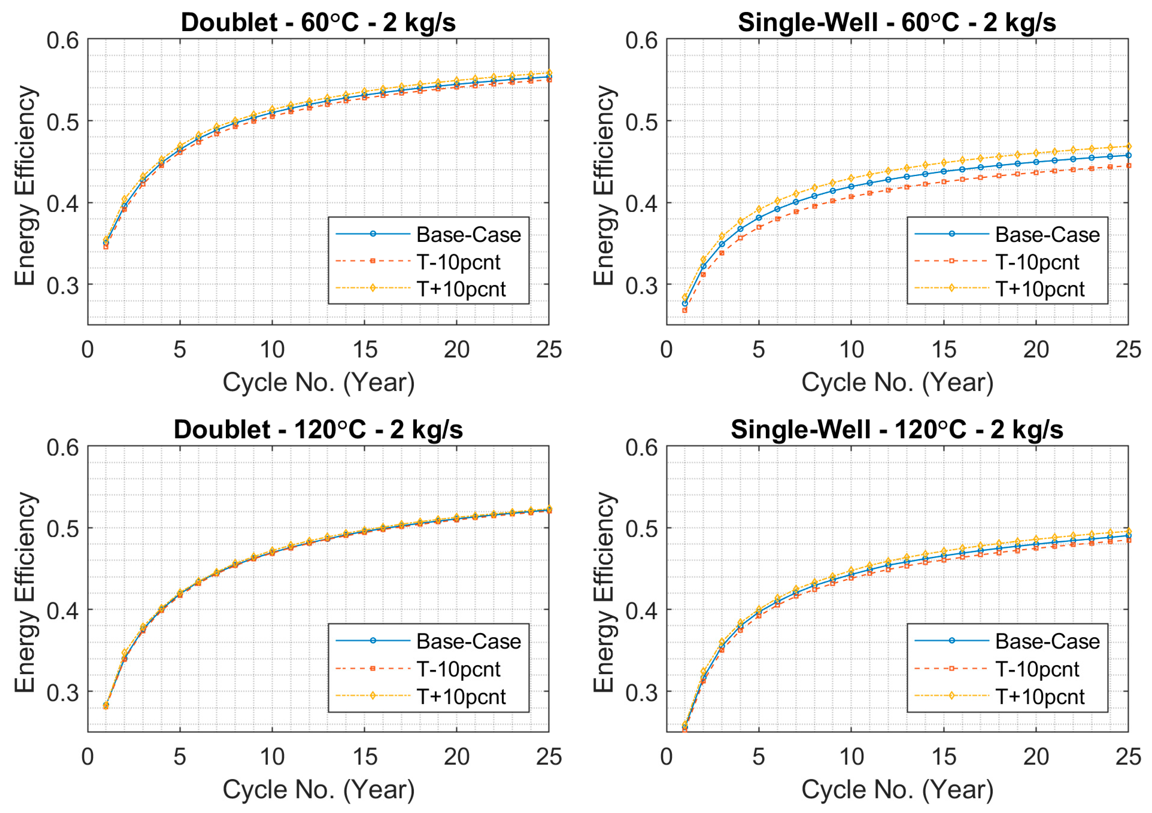
5.3. Sensitivity of Storage Efficiency to Transmissivity Changes
In previous sections, the effect of temperature on fluid viscosity, and consequently on transmissivity changes and system efficiency, was discussed. In this section, different scenarios were modeled by varying initial transmissivity values by +/−10% from the base case at the highest flow rate for both single-well and doublet systems at 60 °C and 120 °C to explore further the impact of initial transmissivity on energy efficiency evolution. The results, as presented in
Figure 10, illustrate the influence of transmissivity adjustments on system performance. As shown in the figure, changes in transmissivity have the most significant impact on the single-well system at 60 °C, where a 10% increase or decrease in transmissivity alters efficiency by approximately 2–3% in the same direction. This highlights the sensitivity of single-well systems to transmissivity variations, particularly at lower injection temperatures. In contrast, the doublet system at 120 °C exhibits the least sensitivity to transmissivity changes, suggesting that there may be a threshold beyond which increased transmissivity no longer enhances system efficiency. A similar pattern is observed in the doublet system at 60 °C, while a 10% reduction in transmissivity slightly decreases efficiency, whereas a 10% increase has very small impact.
The results demonstrate that even slight changes to initial transmissivity can have measurable effects on system efficiency. Additionally, transmissivity can significantly affect the required pumping power during injection and production phases, therefore influencing the overall cost. This indicates the importance of optimizing the reservoir’s initial transmissivity (for example by performing stimulation operations) to achieve efficient heat storage capacity.
5.4. District Heating
The retrieved hot water from the reservoir could be effectively used for district heating in Bedretto village. However, transporting it over 3.6 km can lead to temperature loss, and insulated piping would be necessary to minimize heat loss as well as to prevent the mixing of the hot fluid with tunnel water. In a previous study, Halter et al. [
32] proposed using buried pipes to transport tunnel water directly for residential heat pumps in the village, with an estimated kCHF 800 investment requiring state aid and resident fees. While district heating using the stored energy at the Bedretto reservoir may be challenging, this study demonstrates the system’s potential as a valuable framework for thermal energy storage applications in similar cases. Additionally, district cooling was not considered in this study due to Bedretto’s mild summer temperatures (rarely above 24 °C [
59]), but such a system could also be implemented for future applications in regions where cooling is also needed. The combination of heating and cooling could further increase the system’s efficiency and cost optimization.
5.5. Greenhouse or Other Industrial Heating
An alternative usage for the warm water extracted from the heat storage system at Bedretto is greenhouse heating, and this method can provide stable temperatures for crops. Located at ca. 1470 m elevation in a remote area, Bedretto experiences low air pollution, which can potentially help to reduce the harvest losses caused by the pollution [
78]. The greenhouse structure at Bedretto can address altitude challenges such as wind and snow [
79]. Constructing a greenhouse near the tunnel portal minimizes heat loss during the transportation of the hot water, maintaining average temperatures of about 30 °C initially and reaching over 36 °C in later cycles.
Another potential application for the extracted heat from the Bedretto storage system can be to support industrial processes, similar to the geothermal heat plant in Rittershoffen, France, which was designed to supply heat to an industrial starch plant in Beinheim [
80]. Since June 2016, this plant has consistently provided an average of 22.5 MWth [
80]. A similar approach at Bedretto could utilize the natural water flow from the tunnel during the summer, using a heat pump to meet moderate heating demands [
32], and in winter, when heating requirements increase, the FTES system could provide additional required heat. This combined strategy would provide a reliable and sustainable source of energy.
The analysis of temperature loss between Bedretto village and the nearby greenhouse, as shown in
Figure 9, highlights the importance of proximity and infrastructure design in geothermal heating systems. Shorter pipeline distances to the greenhouse significantly reduce heat loss compared to the village, which shows the need for optimized site selection. Improvements such as increasing the pipe insulation thickness beyond the currently considered 2.5 cm and optimizing the burial depth of the pipes, which is currently set at 0.5 m, have the potential to further reduce heat loss.
5.6. Techno-Economics and Viability of the Technology
The numerical model demonstrated promising results for the energy efficiency of the system, particularly for the doublet configuration at 120 °C, making it comparable with typical HT-ATES systems. While the utilization of the recovered thermal energy is currently limited by the geographic and demographic characteristics of the Bedretto region, this technology has the potential to be more applicable when implemented closer to densely populated areas, where district heating could be the primary application.
The output of ORC (with an estimated average of 10.6 kW) during the winter period is significantly offset by the system’s average pumping power requirements (ca. 21.1 kW) for the same duration, even without accounting for additional heat storage cost during summer and operational expenditures as well as initial capital investments. Given the current efficiencies of ORC technologies, using FTES for electricity generation is economically unfeasible in the presented case study, which shows the need for improved efficiency and cost-reduction strategies.
However, the techno-economic analysis of the district heating model, which was designed based on the most efficient case study (doublet system, with a flow rate of 2 kg/s and injection temperature of 60°), demonstrated the system’s dual advantages by integrating economic and environmental benefits. This approach has the potential to help effectively manage seasonal fluctuations in energy supply and demand as well as reducing CO2 emissions significantly at a relatively lower cost compared with other fossil fuel-based systems.
Furthermore, the emergence of negative electricity prices in Europe [
81], as seen, for example, with 301 h of negative ‘day-ahead market’ pricing in Germany in 2023 [
82], presents a valuable opportunity to significantly reduce the operational costs associated with FTES and, more generally with UTES. Utilizing these negative prices, particularly in summer, could allow for cost-effective hot water injection/storage into reservoirs, therefore improving the economic feasibility of FTES systems.
Also, the presented setup in this study can be further extended into a modular configuration, with multiple, optimally designed injection and production intervals within a single-well or doublet system. Such a modular approach not only increases the flexibility of the system but also allows for dynamic adjustments to the system’s operational parameters depending on the specific conditions. Additionally, the system’s cooling capacity presents significant potential for being implemented in regions where cooling demand is high.
However, it is noteworthy to mention that several challenges must be addressed to assess the overall feasibility of this technology. Initial investment costs, including exploration, drilling, and equipment, may vary from conventional ATES systems due to the complexities associated with fractured reservoirs. Additionally, comprehensive site characterization and precise identification of suitable fractures and faults are critical for successful field applications. Also, an in-depth analysis is necessary to optimize system setup, including well spacing, physical parameters such as density and viscosity, buoyancy effects, fracture/fault selection, and operational parameters, as also suggested by other studies for HT-ATES [
12,
83]. Performing such optimizations can potentially increase energy recovery rates even further in the Bedretto reservoir, and in FTES systems in general, therefore making this approach a promising area for future research and application.
6. Conclusions
This study investigated the potential of faults/fractures in crystalline rock for seasonal heat storage in the context of FTES and proposed a few applications for the use of the retrieved hot water. Using COMSOL Multiphysics, a numerical model was developed for modeling fluid flow and heat transfer in the Bedretto reservoir, incorporating several permeable fault/fracture planes, which are assumed to be further stimulated. The results demonstrated promising energy efficiency for the presented case study, particularly in the doublet configuration, with efficiencies exceeding a maximum of 50% after nine years and reaching above 55% after 25 years. The results indicate that the doublet system consistently achieved higher temperatures and a more uniform thermal front distribution, especially at higher injection temperatures, compared to the single-well setup. Transient temperature profiles showed faster thermal breakthrough at 120 °C, but also increased the risk of efficiency loss. Energy efficiency analyses revealed that, for most cases, higher flow rates improved efficiency, with the doublet system generally outperforming the single-well system. Notably, best storage conditions were found for the doublet system at 60 °C with a flow rate of 2 kg/s. Additionally, it was shown that changes in transmissivity can influence overall system efficiency comparably. The results of LCOE for the proposed solar-PV-powered FTES system for district heating demonstrates its economic viability as a competitive climate mitigation tool compared to conventional energy systems.
This study indicates that FTES offers a promising approach for thermal energy storage, although a number of challenges need to be addressed for optimal implementation of this technology. Key challenges can include initial costs for exploration, drilling, and equipment, alongside the challenge of identifying suitable permeable fractures as also indicated by other studies. Future research should also focus on exploration and fault characterization techniques to investigate the impacts of rock deformation and natural background groundwater flow on the system’s performance, which may be critical to the system’s efficiency and feasibility, especially over longer term.


 ,
, 

