Abstract
Geochemical mapping of river sands in the Manufahi area of Timor-Leste revealed potential areas for future mineral exploration. River sand samples from the study area were collected and geochemically analyzed to identify anomalous concentration distributions of several valuable elements and locate potential target areas and geological formations that may host mineral deposits. The 26 major and minor elements were identified using wavelength-dispersive X-ray fluorescence. The river sands exhibited varying elemental concentrations, with Cr, Cu, Zn, and Ba showing deviations from the normal distribution patterns. Identification of geochemical anomalies is an important task in mineral exploration geochemistry. The mean+2 standard deviations (mean+2STD), median+2 median absolute deviations (median+2MAD), and Tukey’s inner fence (TIF) methods were used to determine the geochemical thresholds. This study shows that TIF and principal component analysis (PCA) methods are highly effective in calculating appropriate threshold values and identifying relevant elemental associations. These approaches have proven useful for delineating target areas for mineral deposits, resulting in reliable outcomes. Four predicted target areas with high potential for deposits and mineralization anomalies of Cr, Cu, Ni, and Ba were delineated in the study area.
1. Introduction
“River sand” is the term used to refer to the samples under analysis in this study [1,2,3]. Fine-to-coarse sand fractions were obtained from the active channel below the water level. Modern river sand is an effective medium for geochemical mapping in many regions worldwide including Japan [4,5], Portugal [6], Brazil [7], and Australia [8]. The characteristics of modern river sands in drainage basins are often influenced by various factors, including source rock lithologies, mineral deposit occurrence, climate, topographic relief, transportation, and depositional environment [8,9,10]. However, the source area materials appear to have the greatest influence on the geochemistry of modern river sands [11,12,13,14,15]. Geochemical data for river sand and other surface sediments often deviate from a normal distribution [16]. The potential occurrence of mineral deposits or atypical lithologies, such as iron-rich sedimentary rocks, radiolarian cherts, carbonatites, and serpentinites, may be responsible for the high elemental concentrations found in river sands [17].
The main duty of the geochemical assessment of mineral resource prospects in the identification of potential areas for further investigation is to determine and separate anomalies, thresholds, and background values [18,19]. Various statistical analyses and methods have been employed using different approaches and parameters, including univariate, bivariate, multivariate, and spatial analyses. These include mean, median, mode, standard deviation, variance, skewness, kurtosis, median absolute deviation (MAD), interquartile range (IQR), Tukey’s inner fence (TIF), mean+2 standard deviations (mean+2STD), median+2 median absolute deviations (median+2MAD), and an association of distribution plots, such as histograms, boxplots, and normal quantile plots, to characterize anomalies and define threshold and background values in a univariate data set that falls outside a normal distribution. Additionally, the Spearman correlation coefficient, principal component analysis (PCA), and inverse distance weighting (IDW) interpolation methods were applied to identify the original geochemical signatures of the source composition and the distribution of anomalies that may be related to mineral deposits or atypical lithologies [19,20,21,22,23,24,25,26,27].
Timor island, as a part of the continent of Australia, is generally characterized by the presence of the significant amount of highly deformed and partially faulted and folded sedimentary, metamorphic, and a few igneous rocks. These rocks vary from the Permian to the Quaternary, and they are associated with allochthonous, para-autochthonous and autochthonous units with affinity to the Asian, Australian, and synorogenic successions. Most of these rocks appear to have undergone significant geological processes, including metamorphism, deformation, volcanic activity, and other tectonic events, both before and after their emplacement in their current positions. These processes occurred during the orogenic phase, leading to the development of thrust faults, overthrust, and the uplift of the territory [28,29,30,31,32,33]. Timor-Leste has an attractive geological setting with well-developed structures and favorable metallogenic conditions, which have led to the discovery of several types of mineral deposits there [34].
The occurrence of mineral deposits is generally associated with the igneous rocks, predominantly mafic and ultramafic in composition. These rocks are well exposed in outcrops, either as rock units associated with several particular formations or as exotic blocks incorporated into the shales and mudstones of the Middle Miocene Bobonaro Complex. Additionally, they also occurred as erosional sediments deposited in ancient fluvial terraces of the Pleistocene–Holocene Ainaro Formation [35,36,37,38,39].
In 1936, mineral exploration activities were conducted across the entire territory of Timor-Leste, including the study area, by Wittouck and the team from Allied Mining Corporation. According to the report by Wittouck [35] on Portuguese Timor Exploration, several potential mineralization areas were discovered and numerous gold nuggets were discovered using the gold panning method. However, no trenching or test pitting was carried out during this project’s mineral exploration.
A recent study by Lay et al. [38] on the Hili Manu chromites reported the occurrence of podiform chromite deposits, along with massive sulfide mineralizations associated with peridotites in ophiolites. In addition, Vicente et al. [39] also identified potential occurrences of chromite mineral deposits associated with peridotites dominated by the Maquelab Complex in the Maquelab area (Oecusse, Timor-Leste).
Several laterite deposits containing Ni and chromite mineralization have also been identified in ophiolites, including those on the islands of Kalimantan, Sulawesi, Maluku, Papua, Tanimbar, Seram, and Buru, as well as in the Philippines [40,41,42,43]. Chromite occurrences in Timor-Leste are comparable to those in Indonesia and the Philippines, reflecting similar geological settings [38,39,44,45].
This study focused on the geochemistry of river sands with the main objective of gathering important information regarding the anomalous concentration distributions of valuable elements and identifying potential target areas and geological formations that may host mineral deposits in the study area. The results of this study can serve as a basis and provide useful information for future geochemical mapping and mineral exploration campaigns in Timor-Leste and similar global geological settings.
2. Geographical and Geological Setting
The territory of Timor-Leste comprises the eastern portion of the island of Timor, the small offshore areas of Atauro Island and Jaco Islet, and the enclave of Oecusse (Figure 1). Geologically, the small island of Atauro is part of the inner Banda arc of the volcanic island. Timor and Jaco Islet are part of the outer Banda arcs and are non-volcanic islands formed by orogenic processes resulting from the collision between the passive margin of the Australian continent and the Banda volcanic arc of the Eurasian plate after the subduction of the Indian Ocean crust [29,32,46,47,48,49]. The study area is geographically located on the south coast of Timor-Leste. The study area is largely characterized by rugged to moderate mountainous topography, with various slopes ranging from moderate to steep. Timor-Leste, including the study area are located in a hot intertropical climatic zone characterized by seasonal monsoons. However, the climate varies across regions due to the significant influence of varying altitudes [50], and it has two distinct seasons: a dry period from June to November and a rainy season from December to May [51,52]. Average annual temperatures and rainfall range from <21 to 25 °C and 2000 to 2500 mm in elevated areas, while in lowland and coastal areas, temperatures range from 25 to 27 °C with annual rainfall between 1500 and 2000 mm [50,53].
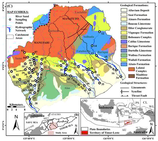
Figure 1.
(A) Geographic map of Timor-Leste and the plate tectonic boundaries of Southeast Asia. Bold greyish-black lines are used to delineate the borders of the Sunda (SU), Australia (AU), Timor (TI), Banda Sea (BS), Molucca Sea (MS), Bird’s Head (BH), Philippine Sea (PS), Caroline (CL), Woodlark (WL), and Maoke (MO) plates (adapted from Bird [54], Pisut [55], Poiata et al. [56]). (B) The geographical location of the study area and its surroundings. The municipalities of Timor-Leste are delineated by heavy black lines (adopted from Pisut [55]). (C) Geological formation map and the distribution of river-sand sampling points in the study area (adapted from Bachri and Situmorang [57], Partoyo et al. [58]).
As delineated by Audley-Charles [28], Bachri and Situmorang [57], and Partoyo et al. [58], along with geological research and mapping carried out by other researchers [32,59,60,61,62,63,64,65,66,67,68,69], the study area encompasses several formations (Figure 1C): (a) Suai Formation, is Pleistocene to the Holocene in age and predominantly consists of rudites and arenites, with minor proportions of mud and marls. These rocks are mainly unconsolidated deposits and typically abundant in foraminifera; (b) Ainaro Formation is Pleistocene to Holocene in age and primarily consists of matrix-supported conglomerates. Ferruginous horizon often caps the irregular upper of these fluvial terrace sediments; (c) Baucau Limestone, which ranges in age from the Lower Pleistocene to the Holocene, primarily consists of coral-reef limestones, along with minor amounts of calcarenites, calcirudites, and conglomerates. Massive coral growths are the predominant components of coral reef limestones; d) Dilor Conglomerate, composed of sandstones and conglomerates with significant detritus input from the quartzites of the Lolotoi Complex, is Pliocene in age; (e) Viqueque Formation, dating from the Upper Miocene to the Lower Pliocene, is lithologically divided into two sections: (i) the upper layer comprises significant proportions of silty marls, marly siltstones, silty claystones, siltstones, and sandstones, as well as lesser calcilutites and biocalcarenites; (ii) the lower layer contains minor proportions of basal conglomerates and mottled marls, along with notable amounts of marls, clayey marls, silty marls, calcilutites, and tuffs; (f) Bobonaro Complex, Middle Miocene in age, is dominated by exotic blocks within a scaly clay matrix. The matrix lithology resembles that of the mudstone of the Wailuli Formation. Exotic blocks that are Permian to Cretaceous in ages are common and extensively distributed; (g) Cablac Limestone, ranging in age from the Oligocene to the Miocene, predominantly consists of oolitic and peloidal limestones, pelagic carbonates, and minor proportions of intraformational conglomerates, calcilutites, calcarenites, agglomerates, and tuffaceous rocks; (h) Barique Formation is Oligocene in age and is primarily composed of mafic to acidic lavas and tuffs, with lesser amounts of serpentinites, volcanic conglomerates, and sandstones; (i) Dartollu Limestone, which has been dated to the Middle–Upper Eocene, is largely composed of algal and alveolina biomicarenites, with minor amounts of calcilutites, siliceous shales, and siltstones; (j) Waibua Formation ranges in age from the Lower to the Upper Cretaceous and mainly consists of radiolarites, radiolarian cherts, marls, and shales, with varying proportions of calcilutites, marls, and calcarenites; (k) Wailuli Formation, in which the major constituents include gray shales and blue-gray marls, with lesser amounts of sandstones, mudstones, quartz-arenites, coarse polymictic conglomerates, calcarenites, and calcilutites, is Late Triassic to Middle Jurassic in age. Most shales are characterized by fine micaceous minerals and microcrystalline carbonates, with small amounts of pyrite; (l) Aitutu Formation, which ranges in age from the Middle to Upper Triassic, is largely composed of calcilutites, shales, and calcareous shales with minor proportions of marls, calcarenites, lumachelles, quartz-arenites, radiolarites, bituminous rocks, and cherts. Several limestones have undergone silicification, dedolomitization, and pyritization processes; (m) Lolotoi Complex mainly consist of metamorphosed sedimentary and volcanic rocks, as well as basic to ultrabasic and felsic volcanic rocks. They are mostly greenschists, phyllites, amphibolite, garnet-bearing pelitic gneisses and schists, metagabbros, garnet mica schists, mafic and felsic igneous dikes, pelitic schists, metabasite schists, carbonate-rich greenschists, and peridotites [28,32,68,69]. Most metamorphic rocks within the Lolotoi Complex are derived from sedimentary rocks. Several meta-volcanic rocks have been extensively altered and they frequently occur in association with meta-sedimentary rocks. The Lolotoi Complex was emplaced to their current allochthonous position as flat thrust sheets (klippen) and this complex dates from the Triassic to the Late Cretaceous; and (n) Maubisse Formation, which is Permian in age, largely comprises fossiliferous limestones and volcanic rocks, along with well-bedded dense biocalcarenites, massive reef limestones, pink crinoidal limestones, calcirudites, sandstones, calcareous shales, micaceous siltstones, tuffs, volcanic conglomerates, basalts, marbles, and metamorphosed basic volcanics.
3. Samples and Methods
3.1. Sampling and Preparation
In this study, basic procedures for sampling river sand and treating samples before chemical analysis, as outlined in Hale and Plant [70], Darnley et al. [71], Tanaka et al. [72], Fletcher [73], Ohta et al. [74], and Yamamoto et al. [5], were implemented. Modern river sand samples were collected from 53 sites in the study area (Figure 1). Samples were dried in an oven at 105 °C and then sieved using a vibrating sieve shaker machine (VSS-200S Type, Tsutsui Scientific Instruments Co., Ltd., Tokyo, Japan). The composite samples of fine-grained river sands sieved through 180–150 and <150 μm metal sieves were ground using an agate mortar and pestle, followed by machine crushing using an agate ball mill (Vibrating ball mill machine, ITO Seisakusho Co., Ltd., Yokkaichi, Japan). Moisture and volatile materials, consisting of “combined water” (hydrates and labile hydroxy-compounds) and carbon dioxide from carbonates, were removed from the samples using the loss-on-ignition method [75]. The removal was quantified by measuring the weight loss of the samples before and after heating them to 950 °C.
As described and recommended by Yamamoto and Morishita [76], to analyze major and minor elements, glass beads were used for sample preparation in X-ray fluorescence (XRF) analysis. The fused glass beads were prepared by mixing the powder at a sample-to-flux ratio of one to two after heating. The flux used was a white crystalline powder of lithium tetraborate (Li2B4O7 = 169.12). The mixed powder was placed in a platinum crucible and processed using a bead sampler (TK-4100 model, Amena Tech Co., Yokohama, Japan) to form glass beads.
3.2. Analytical Methods and Data Analysis
Fifty-three modern river sand samples were analyzed using wavelength-dispersive XRF (WD-XRF) at the Division of Instrumental Analysis, Gifu University, and 26 major and minor element concentrations were determined. These elements were accurately calibrated using standard reference samples provided by the Geological Survey of Japan (GSJ).
3.2.1. Univariate Analysis
In this study, basic and classical descriptive statistics refer to univariate analyses, which include the calculation and estimation of minimum, maximum, mean, mode, median, variance, range, standard deviation, and quartile values. In addition to the aforementioned parameters, skewness and kurtosis were also employed as initial estimates to indicate the distribution characteristics of the studied geochemical elements. In normal distributions, the skewness is zero and the kurtosis is approximately three, whereas the mean, mode, and median values are nearly identical [77,78,79,80]. In addition, statistical methods such as mean+2STD, median+2MAD, and TIF are the most precise methods for defining anomaly threshold values, proving more effective and straightforward than other approaches. In certain cases, where the raw geochemical data did not follow a normal distribution, the mean+2STD method failed to provide a relevant threshold estimate. The TIF method was calculated using the formula: [TIF = Q3 + 1.5 × IQR], where the third quartile (Q3) represents the 75th percentile value (Q75), and interquartile range (IQR) represents the difference between the 75th and 25th percentile values (Q3-Q1) [19,20,22,81,82,83,84].
The distribution plots, which involve the joint application of several graphs and diagrams, such as normal quantile plots, boxplots, and histograms, are focused on visualizing, simplifying, and clarifying the distribution and characteristics, or any deviations, in the studied geochemical elements that could be attributed to the contributions of the underlying lithologies or mineral deposits [80,85,86,87]. The boxplot method is also one of the most precise approaches for defining anomaly thresholds in exploration targeting, particularly when dealing with complex geochemical data, including non-normal distributions, spatial heterogeneity, and background variability. This approach identifies outliers as values falling beyond 1.5 or 3 times the interquartile range (IQR) above the third quartile or below the first quartile, helping in the detection of outliers or extreme values within a distribution and making it especially effective for skewed geochemical data. Figure 2 shows the elements of boxplot, which categorizes a set of geochemical element data into five reliable classes as follows [85]: (a) the lowest-lower whisker is classified as extremely low background; (b) lower whisker-lower hinge is labelled as low background; (c) lower hinge-upper hinge is defined as background; (d) upper hinge-upper whisker is considered high background; and (e) upper whisker-highest is classified as an anomaly. In addition, the upper inner fence was defined as the threshold for separating the background from anomalous values.
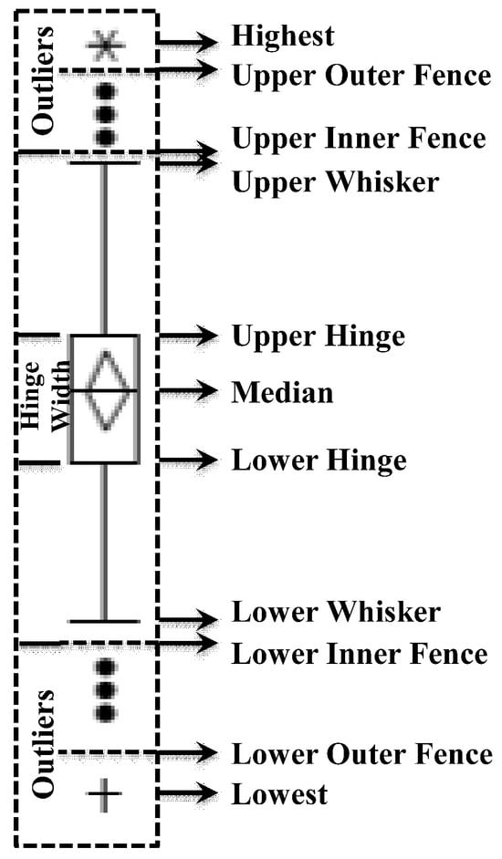
Figure 2.
Schematic features of a boxplot.
3.2.2. Bivariate and Multivariate Analyses
The Spearman correlation coefficient was employed to identify and evaluate the inter-relationships between the variables of the geochemical elements that deviated from a normal distribution. This approach is more effective than the Pearson correlation coefficient, which is sensitive to outliers and can potentially distort the results [88]. PCA is one of the most commonly used techniques for multivariate statistical analyses and is an effective and reliable approach for extracting information and determining the composition of geochemical populations [9,23,89], outlining the source composition of underlying lithologies and identifying areas of interest for the potential occurrence of mineral deposits [27,90]. Only principal components with eigenvalues greater than or near 1.0 were used to analyze and interpret PCA results in a biplot of joint graphical representations of variables and samples because they represent most of the variance in the data [82,91,92]. IDW is a deterministic, predictable, and reproducible approach for multivariate spatial techniques that can be applied to compute and interpolate values in areas where samples were not collected. IDW assigns more influence on the interpolated value to the points closest to the known value points than to those farther away [93]. In this study, IDW was employed to create a surface model that represented the spatial distribution of multi-element associations derived from the PCA scores along with several independent variables.
Descriptive statistics, distribution plots, Spearman’s correlation coefficients, and PCA were performed using Microsoft Office Excel version 2405 (Build 17628.20144) and JMP Pro 14. Additionally, the maps presented in this study, including interpolated and geological maps, were created using ArcGIS 10.4.
4. Results
4.1. Statistical and Distribution Characteristics of Geochemical Elements
The basic and classical descriptive statistics of the univariate analysis of the 26 raw geochemical elements in river sands from the study area are summarized in Table 1. In this study, we present geochemical analysis results for both major and minor elements. However, our focus was on minor elements, as the geochemical characteristics of the major elements regarding their provenance have already been discussed and published [94].

Table 1.
Descriptive statistics for raw geochemical elements in river sands from the study area. All major element concentrations are given in weight percent (wt.%), and minor element contents are measured in parts per million (ppm).
Table 1 presents the skewness and kurtosis values, which reveal that TiO2, Fe2O3, MnO, K2O, CaO, Cr, Cu, Zn, and Ba exhibited values higher than zero, whereas the remaining elements displayed skewness or kurtosis values lower than zero. Table 1 also documents the geochemical threshold values used to separate anomalies from background values for the 26 elements in river sands from the study area. These threshold values were determined using the mean+2STD, median+2MAD, and TIF methods. Anomaly threshold values obtained from statistical approaches that exceeded the maximum measured values were excluded. Nb had a threshold value determined by the median+2MAD approach, whereas SiO2, Al2O3, Na2O, Co, Ga, Sr, Y, Zr, Nb, and Th had threshold values obtained from the mean+2STD method, which were greater than the maximum measured values. In addition, TiO2, CaO, Cr, Cu, Zn, and Ba exhibit threshold values lower than the maximum values derived from the TIF approach.
To complement the descriptive statistics, distribution plots for the raw geochemical data of the river sands were generated. The distribution plots for Cr, Cu, Zn, and Ba are presented in Figure 3 and those for the remaining elements are provided in the (Appendix A, Figure A1 and Figure A2). The distribution plots for the analyzed geochemical elements primarily exhibited a normal distribution; however, those for Cr, Cu, Zn, and Ba deviated from the normal distribution.
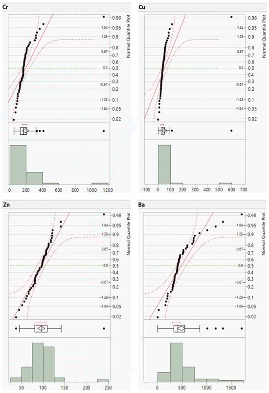
Figure 3.
Distribution plots of Cr, Cu, Zn, and Ba concentrations (in ppm).
4.2. Correlation and Multi-Element Relationships
The Spearman correlation coefficients between any pair of variables (elements) for the sampled river sands are presented in Table 2. The PCA results for the variables are presented in Table 3 and depicted in the component pattern biplot of the first four principal components, as shown in Figure 4 and Figure 5 (A and B). The percentages of variance explained by the first, second, third, and fourth principal components were 56.04%, 13.10%, 7.72% and 5.63%, respectively. PC1 exhibited strong positive relationship with Ga, Co, Y, La, Pb, Th, Al2O3, Nb, Zr, Ni, Rb, MgO, Fe2O3, Na2O, P2O5, Zn, SiO2, Sc, Cr, TiO2, and K2O. In contrast, the negative PC1 scores had strong loadings for CaO and Sr. K2O, SiO2, Rb, Ba, and Zn showed relative enrichment in the positive values of PC2, while the negative PC2 scores were strongly associated with Sc, MgO, Fe2O3, Cr, and TiO2. MnO, Ba, and TiO2 showed strong positive correlations with PC3, while the negative PC3 values were strongly associated with Cu and Zn. In addition, PC4 exhibited strong positive correlations with Cu, Sr, Zn, and MnO.
Table 2.
Non-parametric correlation coefficient (Spearman) between geochemical elements in the river sands from the study area. The correlations between elements discussed in the text are denoted by boldface type.
Table 3.
Variable results of the PCA for the first four components with eigenvalues greater than 1.0. Loading values are presented for variables with values greater than +0.3 and less than −0.3.
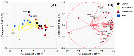
Figure 4.
Samples (A) and variables (B) plotting on the first two component axes of the principal component analysis (PCA).
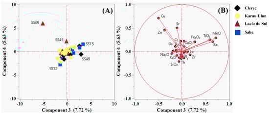
Figure 5.
Samples (A) and variables (B) plotted on the third and fourth component axes of the PCA.
Table 4 presents the results derived from the PCA analysis of the samples. According to the results, samples SS23, SS1, SS41, SS50, SS42, SS40, SS45, and SS48, which exhibited high loading values greater than 5.0, showed strong positive associations with the first principal component. These samples are located in the upstream areas of the northern and northwestern branches of the Karau Ulun River, as well as in the upstream areas of the Laclo do Sul and Clerec Rivers, suggesting a predominance of carbonate rocks. In contrast, the negative values of PC1 were strongly associated with samples SS29, SS15, SS4, SS6, and SS30, which showed low loading values of less than −5.0. These samples were collected from basins located in the midstream areas of the Karau Ulun River’s north-nortwest branches and midstream area of the Sahe River, demonstrating a dominance of non-carbonate rocks. The positive values of the second principal component showed great relationships with samples SS49, SS39, SS12, SS43, SS9, and SS13, all of which had high loading values exceeding 2.0. These samples were collected from the midstream areas of the Laclo do Sul, Clerec, and Sahe Rivers, as well as upstream area of the Sahe River. On the other hand, samples SS4, SS45, SS11, SS29, and SS50, which displayed low loading values below −2.0, were located in the midstream areas of the Karau Ulun River’s north-nortwestern branches and in the midstream areas of the Laclo do Sul and Clerec Rivers. These results indicate that mafic-rich rocks either dominate or are absent in these basins. Sample SS39 was strongly associated with the negative values of PC3, whereas the positive PC3 scores showed strong correlations with samples SS15, SS49, SS13, and SS50. These samples were collected from the midstream areas of the Sahe, Clerec, and Laclo do Sul Rivers, indicating the potential presence of rocks with or without Cu-Zn mineralization.
Table 4.
Sample results for the first four components of the PCA. Loading values for samples with values greater than +2.0 and less than −2.0 are shown in bold.
Furthermore, samples SS039 and SS045 have strong positive correlation with fourth principal component, suggesting the presence of a mineralization-forming environment in these basins.
5. Discussion
5.1. Geochemistry and Provenance of River Sands
The concentration ranges of minor elements in Earth surface materials, as presented by Kabata-Pendias and Mukherjee [95], are provided in the (Appendix A, Table A1) and can be used as references for the study area. Certain minor elements in basic rocks have higher concentrations than those in argillaceous rocks and sandstones, and vice versa. The basic and ultramafic rocks are identified by a significant percentage of mafic minerals [96], which typically contain higher concentrations of Cr, Co, Ni, Cu, and Sc [95,97]. In the basic and ultramafic igneous rocks, the values of Cr, Co, Ni, Cu, Nb, and Sc range from 170–3400, 35–200, 130–160, 10–120, 10–35, and 5–35 ppm, respectively. In addition, argillaceous rocks are characterized by a significant proportion of clay minerals [98]. However, carbonate materials are also abundant and have been found to be integrated into sediment and sedimentary rocks in different proportions [99].
The concentrations of Zn, Ga, Rb, Sr, Ba, Pb, Th, and La in the argillaceous sedimentary rocks range from 80–120, 15–25, 120–200, 300–450, 500–800, 14–40, 10–12, and 30–90 ppm, respectively. The values of Y and Zr in the sandstones vary from 15–250 and 180–250 ppm, respectively.
The high concentrations of Cr are probably related to the presence of the mafic minerals rich lithologies with or without chromite deposits. In addition, the elevated concentrations of Cu and Zn recorded in the river sands within the study area are possibly related to the occurrence of rocks with Cu-Zn deposits [39,100]. Ba, Sr, and Rb are widely recognized as mobile elements that are often depleted in river sands because of their mobility and leachability during weathering [101,102]. However, the high concentrations of Sr and Ba measured in the study area are likely due to the presence of the barite minerals occurring within carbonate-rich lithologies associated with hydrothermal processes [39,103].
The Spearman correlation coefficient results (Table 2) revealed that the contribution from the destruction of carbonate, clay, mica, and feldspar minerals was reflected in the negative correlation between most of the minor elements and Sr and CaO, significant positive associations between most minor elements and Ga and Al2O3, and significant positive correlations between K2O and Rb and Pb and Rb. Ba displayed a positive relationship with K2O, Rb, and Sr. Moderate-to-strong positive associations were observed among Cr, Co, Ni, Sc, TiO2, Fe2O3, and MgO, likely reflecting the contributions of minerals such as chromite, garnet, olivine, pyroxene, amphibole, sphene, rutile, hematite, ilmenite, magnetite, biotite, and chlorite to the river sand compositions.
The major contributions of clastic sedimentary rocks (such as shales, claystones, siltstones, and mudstones), mafic igneous rocks with chromite deposits, carbonate sedimentary rocks, metamorphic rocks, and Cu-Zn deposits in the river sands were confirmed by observing the distribution plots of minor elements (Figure 3 and Appendix A, including Figure A1 and Figure A2), comparing the concentrations of minor elements with the range in concentrations presented by Kabata-Pendias and Mukherjee [95], and the results of the Spearman correlation coefficient [97,100,104,105,106]. The potential occurrence of hydrothermal and metamorphic processes, along with the presence of clastic and carbonate sedimentary, igneous, and metamorphic rocks in the study area, has been reported by Vilanova et al. [94].
The PCA results indicated that the pattern plot of PC1 and PC2 (Table 3 and Table 4; Figure 4) defined the geochemical associations of elements related to the origin and composition of the underlying lithologies, whereas PC3 and PC4 (Table 3 and Table 4; Figure 5) allowed identification of the presence and distribution of a mineralization-forming environment in the study area. The PCA findings corroborate the aforementioned results.
The pattern plot of PC1 may effectively separate the presence and distribution of compositional variations between the carbonate- and non-carbonate-rich river sands from the study area. Carbonate minerals associated with carbonate sedimentary rocks or carbonate-rich lithologies whose source rock derives from a carbonated environment, may have significantly contributed to the elemental association observed in the negative scores of PC1. This component was prominently recorded at sample locations SS29, SS15, SS4, SS6, and SS30, which were mainly drained from the Aitutu, Viqueque, and Wailuli Formations. The elemental relationship seen in the positive values of PC1 may have been strongly influenced by non-carbonate minerals, such as clay, mica, quartz, feldspar, heavy, and other accessory minerals commonly found in clastic sedimentary rocks. These rocks are sourced from both continental and oceanic parent rocks, which are often associated with active tectonic environments. The elemental association observed in these positive values was highly concentrated in sample locations SS23, SS1, SS41, SS50, SS42, SS40, SS45, and SS48, which were primarily drained from the Wailuli, Viqueque, and Aitutu Formations, as well as the Bobonaro Complex. The PC2 pattern plot effectively captures the compositional variations between the mafic- and non-mafic-rich river sands in the study area. The negative PC2 scores reflect contributions from chromite, garnet, spinel, olivine, pyroxene, amphibole, biotite, magnetite, sphene, ilmenite, and chlorite minerals, which are associated with mafic environment characteristics or clastic sedimentary rocks derived from predominantly oceanic parent rocks typical of active tectonic regions. Representing this component, samples SS4, SS45, SS11, SS29, and SS50 were collected from areas drained from the Lolotoi and Bobonaro Complexes as well as from the Ainaro, Viqueque, and Wailuli Formations. The basic rocks associated with the Bobonaro Complex were identified as exotic blocks that were incorporated into clastic sedimentary rocks (such as shales and mudstones) [107]. The elemental association observed in the positive values of PC2 was potentially consistent with the relative abundance of feldspar, quartz, mica, and clay minerals in the river sands. These minerals can be attributed to the presence of acidic rock compositions or clastic sedimentary rocks sourced from major contributions of Australian continental plate. The elemental relationship observed in these positive scores was highly reported in samples SS49, SS39, SS12, SS43, SS9, and SS13, which were collected from areas drained from the Wailuli Formation.
5.2. Influence of Mineral Deposit Potential on the Geochemical Characteristics of River Sands
The statistical parameters of the raw geochemical elements, particularly skewness and kurtosis, indicated that Cr, Cu, Zn, and Ba had values greater than 1 and 3, respectively. These elements also exhibited relatively noticeable differences in the mean, median, and mode values. For CaO, the skewness value was greater than 1, whereas the kurtosis value was less than 3. The threshold values for TiO2, CaO, Cr, Cu, Zn, and Ba were obtained using these three methods. The threshold values achieved by the methods followed the decreasing order TIF > mean+2STD > median+2MAD for TiO2 and CaO, whereas Cr, Cu, Zn, and Ba decreased in the order mean+2STD > TIF > median+2MAD. The TIF approach values corresponded closely to the upper inner fence values of the boxplot [81,82,108], and the results of this approach were used as the threshold values [83,84].
Five geochemical classes for the concentrations of Cr, Cu, Zn, and Ba were identified using the boxplot model [85], as shown in Table 5. A distribution map of geochemical classes for Cr, Cu, Zn, and Ba in the study area was delineated using the IDW method for gridding and illustrating the spatial distributions of geochemical anomalies (Figure 6). Anomalous values of Cr were observed in the midstream to downstream areas of the Laclo do Sul River basin. In contrast, anomalous values of Ba were concentrated in the northern branch of the Clerec River catchment, midstream areas of the Sahe River basin, and midstream areas of the western branch of the Karau Ulun River catchment. In addition, the nearly identical spatial distribution patterns of Cu and Zn likely indicated that they were derived from the same source materials [109]. Anomalous values of Cu and Zn were observed in the midstream area of the Laclo do Sul basin.
Table 5.
Geochemical classes derived from the boxplot model for Cr, Cu, Zn, and Ba concentrations (in ppm) in river sands from the study area.
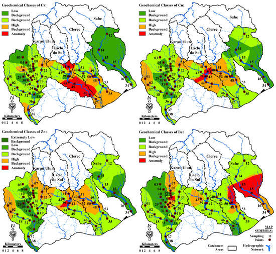
Figure 6.
Distribution of geochemical classes for Cr, Cu, Zn, and Ba in the study area, derived from the boxplot model.
The positive PC3 and PC4 values as well as the negative PC2 and PC3 scores were subjected to distribution plots (Figure 7) to separate the five geochemical populations with extremely low background, low background, background, high background, and anomalies (Table 6). Five distinct geochemical classes were delineated using the IDW approach for gridding and illustrating the spatial distributions of anomalous values from the selected PCA components in the study area (Figure 8).
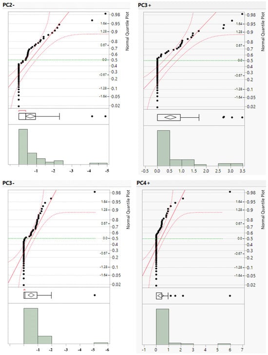
Figure 7.
Distribution plots of the positive PC3 and PC4 scores, as well as the negative values of PC2 and PC3.
Table 6.
Geochemical classes derived from the boxplot models for the positive PC3 and PC4 scores and negative values of PC2 and PC3.
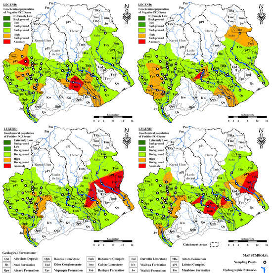
Figure 8.
Distribution of geochemical anomalies for the elemental association of the negative PC2 and PC3, as well as the positive PC3 and PC4 values, derived from the boxplot model.
Sc, MgO, Fe2O3, Cr, and TiO2 were grouped together on the negative side of PC2, likely reflecting the presence of mafic, heavy, and accessory minerals concentrated in the igneous and metamorphic rocks [100,106,110]. However, the high anomalous value distributions of Cr and elemental associations in the negative PC2 scores (Figure 6 and Figure 8) may be related to the presence of igneous rocks (basic and ultramafic) containing chromite mineral deposits [39,94]. The samples representing these anomalies were collected from areas that were drained from the Lolotoi and Bobonaro Complexes, particularly in the upstream areas of the northwestern branch of the Karau Ulun River catchment and the midstream areas of the Laclo do Sul basin. The existence of igneous rocks with chromite mineral deposits associated with the Bobonaro Complex as exotic blocks were incorporated into shales and mudstones [107].
The occurrence of a potential mineralization zone dominated by Cu and Zn could explain their high anomalous value distributions, as well as the elemental relationships in the negative PC3 scores [100,105], in the midstream areas of the Laclo do Sul River basin (Figure 6 and Figure 8). This anomaly is particularly evident in the sample drained from rocks dominated by the Wailuli Formation, which could be the host rocks for the Cu-Zn mineralization.
Overall, the contributions of carbonate and muscovite were most likely responsible for the presence and distribution of Ba [97,104] in the river sands of the study area. However, the high anomalous value distributions of Ba and the elemental association of MnO-Ba-TiO2 in the positive PC3 scores likely indicate the occurrence of secondary alteration mineral assemblages associated with mineralization and formation of barite, rutile, goethite and Mn-bearing minerals [39,111]. The distribution of geochemical classes for positive PC3 values in the study area shows that anomalous values of this component were concentrated in the northern branch and downstream areas of the Clerec River catchment, as well as in the midstream areas of the Sahe River basin (Figure 8). Samples carrying these anomalies were collected from locations drained from rocks dominated by the Aitutu and Wailuli Formations, which may contain hydrothermal mineralizations.
The elemental associations reflected in the positive PC4 scores could be significantly influenced by the presence of Cu-Zn deposits, as well as carbonate and manganese minerals [39,100,105]. Anomalous values of this component were identified in the midstream areas of the Laclo do Sul, Clerec, and Sahe River catchments (Figure 8). These anomalies were most pronounced in samples derived from rocks dominated by the Aitutu and Wailuli Formations, along with the Bobonaro Complex, indicating potential mineralization-related environments.
5.3. Prediction of Target Areas for Future Research and Exploration
Four potential target areas for mineral deposits were identified in the study area and proposed for further study and exploration, as illustrated in Figure 9. Target areas A and B show evident distributions of anomalous values of Cr and elemental assemblages with the negative PC2 scores, as shown in Figure 6 and Figure 8. The distributions of anomalous values of Cu and Zn as well as the elemental association with negative PC3 scores (Figure 6 and Figure 8), corresponded well with the delineation of target area C. In addition, the proposed boundary of target area D is consistent with the distribution of anomalous Ba values and anomalous scores of multi-element relationships in the positive PC3 and PC4.
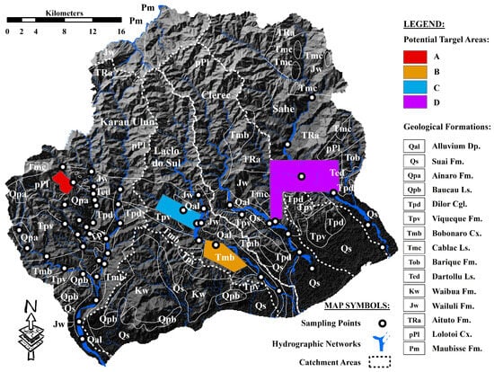
Figure 9.
Proposed potential target areas for mineral deposits in the study area.
6. Conclusions
The characteristics of Cr, Cu, Zn, and Ba in the river sands of the study area fell outside a normal distribution. The threshold estimated for these elements using the mean+2STD approach failed to yield adequate values, whereas the median+2MAD method delivered low threshold values, leading to the detection of the greatest number of outliers. This study presents the findings that the TIF and PCA methods are highly applicable and effective for calculating appropriate geochemical thresholds to separate anomalies from background values and identify relevant elemental associations. These approaches have proven useful for delineating target areas for mineral deposits, resulting in reliable outcomes [83,84,112,113].
The geochemical analysis of the river sand samples across the study area reveals substantial variation in element concentrations, pointing to a complex interplay of geology, lithology, and mineralogy. Anomalies of Cr and Ba in midstream areas of the Laclo do Sul and Sahe Rivers align with the presence of mafic minerals rich lithologies with or without chromite deposits and carbonate rocks, while elevated Cu and Zn concentrations suggest potential Cu-Zn mineralization zones, especially within the Wailuli and Aitutu Formations. Additionally, anomalies and elevated concentrations of Ba and Mn in several areas could be associated with the presence of barite and manganese minerals, which may be indicative of hydrothermal activity. Geochemical evidence, lithological compositions, and anomalous geochemical distributions underscore the presence and distributions of mineralization-forming environment associated with the Lolotoi and Bobonaro Complexes, as well as the Aitutu and Wailuli Formations. These geological formations sourced from both continental and oceanic parent rocks typical of active tectonic regions and are possible prospective for hosting economically viable mineral deposits.
The occurrence of hydrothermal mineralization associated with the Gondwana Megasequence has been reported previously by Vicente et al. [39]. Further geochemical investigations and mineral exploration campaigns are recommended in areas underlain by the Wailuli Formation, particularly within the proposed boundaries of Target Area D (Figure 9). This area is considered a potential source of the detected Ba geochemical anomalies and may provide evidence of significant hydrothermal alteration of the associated rocks.
Author Contributions
V.V.: conceptualization, methodology, validation, investigation, formal analysis, writing—original draft. T.O.: validation, supervision, visualization, writing—review and editing. S.K.: validation, supervision, visualization, writing—review and editing. K.Y.: formal analysis. E.M.: investigation, formal analysis. All authors have read and agreed to the published version of the manuscript.
Funding
The Japan International Cooperation Agency (JICA) Development Studies Program, Human Resources Development in Science and Technology Innovation, and the Earth Science Laboratory, Faculty of Engineering, Gifu University provided funding for this study and covered the article processing charges (APC).
Data Availability Statement
All data included or referenced within this article are publicly available.
Acknowledgments
This study was made possible through the generous financial support of the Japan International Cooperation Agency (JICA) Development Studies Program and Human Resources Development in Science and Technology Innovation. We express our sincere appreciation to the staff of the Ministry of Petroleum and Mineral Resources, particularly Instituto de Geociências de Timor-Leste and the National Petroleum and Minerals Authority, Dili, Timor-Leste, for authorizing the shipment of samples from Timor-Leste to Japan. We also extend our gratitude to Nagayoshi Katsuta and Yuma Masuki of Gifu University for allowing us to take advantage of their laboratory facilities to prepare the glass bead samples. Finally, we would like to extend our heartfelt gratitude to the Nagoya University Museum, JICA and the dedicated staff members of the Faculty of Engineering at Gifu University, Koshi Yamamoto, Koichi Shimakawa, Atsushi Takahashi, Mieko Araki, Yukiko Eguchi, Naoko Yamada, and Midori Iinuma.
Conflicts of Interest
The authors declare that there are no conflicts of interest, either financial or non-financial, that might affect the topic or findings of the research presented in this paper.
Appendix A


Figure A1.
Distribution plots of major element concentrations (in wt.%).


Figure A2.
Distribution plots of minor element concentrations (in ppm).
Table A1.
The abundance range values of minor elements in argillaceous, sandstone, and basic to ultramafic rocks (data from Kabata-Pendias and Mukherjee [95]).
Table A1.
The abundance range values of minor elements in argillaceous, sandstone, and basic to ultramafic rocks (data from Kabata-Pendias and Mukherjee [95]).
| Minor Elements | Basic-Ultramafic Igneous Rocks (in ppm) | Argillaceous Sedimentary Rocks (in ppm) | Sandstones (in ppm) |
|---|---|---|---|
| Cr | 170–3400 | 80–120 | 20–40 |
| Co | 35–200 | 14–20 | 0.3–10 |
| Ni | 130–160 | 40–90 | 5–20 |
| Cu | 10–120 | 40–60 | 5–30 |
| Zn | 40–120 | 80–120 | 15–30 |
| Ga | 15–24 | 15–25 | 5–12 |
| Rb | 2–45 | 120–200 | 10–45 |
| Sr | 140–460 | 300–450 | 20–140 |
| Y | 0.5–20 | 25–40 | 15–250 |
| Zr | 80–200 | 160–200 | 180–250 |
| Nb | 10–35 | 15–20 | 0.5–10 |
| Ba | 250–400 | 500–800 | 100–320 |
| Pb | 0.1–8 | 14–40 | 5–10 |
| Th | 1–14 | 10–12 | 2–4 |
| Sc | 5–35 | 10–15 | 1–3 |
| La | 2–70 | 30–90 | 17–40 |
References
- Franzinelli, E.; Potter, P.E. Petrology, Chemistry, and Texture of Modern River Sands, Amazon River System. J. Geol. 1983, 91, 23–39. [Google Scholar] [CrossRef]
- He, J.; Garzanti, E.; Jiang, T.; Barbarano, M.; Resentini, A.; Liu, E.; Chen, S.; Shi, G.; Wang, H. Mineralogy and Geochemistry of Modern Red River Sediments (North Vietnam): Provenance and Weathering Implications. J. Sediment. Res. 2022, 92, 1169–1185. [Google Scholar] [CrossRef]
- Liang, W.; Hu, X.; Garzanti, E.; Wen, H.; Hou, M. Petrographic Composition and Heavy Minerals in Modern River Sand: A Global Database. Geosci. Data J. 2023, 11, 443–451. [Google Scholar] [CrossRef]
- Tanaka, T.; Kawabe, I.; Hirahara, Y.; Iwamori, H.; Mimura, K.; Sugisaki, R.; Asahara, Y.; Ito, T.; Yarai, H.; Yonezawa, C.; et al. Geochemical Survey of the Sanaga-Yama Area in Aichi Perfecture for Environmental Assessment. J. Earth Planet. Sci. Nagoya Univ. 1994, 41, 1–31. [Google Scholar]
- Yamamoto, K.; Tanaka, T.; Minami, M.; Mimura, K.; Asahara, Y.; Yoshida, H.; Yogo, S.; Takeuchi, M.; Inayoshi, M. Geochemical Mapping in Aichi Prefecture, Japan: Its Significance as a Useful Dataset for Geological Mapping. Appl. Geochem. 2007, 22, 306–319. [Google Scholar] [CrossRef]
- Dinis, P.A.; Sequeira, M.; Tavares, A.O.; Carvalho, J.; Castilho, A.; Pinto, M.C. Post-Wildfire Denudation Assessed from Compositional Features of River Sediments (Central Portugal). Appl. Clay Sci. 2020, 193, 105675. [Google Scholar] [CrossRef]
- Vital, H.; Stattegger, K. Major and Trace Elements of Stream Sediments from the Lowermost Amazon River. Chem. Geol. 2000, 168, 151–168. [Google Scholar] [CrossRef]
- Nesbitt, H.W.; Young, G.M.; McLennan, S.M.; Keays, R.R. Effects of Chemical Weathering and Sorting on the Petrogenesis of Siliciclastic Sediments, with Implications for Provenance Studies. J. Geol. 1996, 104, 525–542. [Google Scholar] [CrossRef]
- Grunsky, E.C.; Drew, L.J.; Sutphin, D.M. Process recognition in multi-element soil and stream-sediment geochemical data. Appl. Geochem. 2009, 24, 1602–1616. [Google Scholar] [CrossRef]
- Johnsson, M.J. The System Controlling the Composition of Clastic Sediments. Geol. Soc. Am. 1993, 284, 1–21. [Google Scholar]
- Cocker, M.D. Geochemical Mapping in Georgia, USA: A Tool for Environmental Studies, Geologic Mapping and Mineral Exploration. J. Geochem. Explor. 1999, 67, 345–360. [Google Scholar] [CrossRef]
- Oliva, P.; Viers, J.; Dupré, B. Chemical Weathering in Granitic Environments. Chem. Geol. 2003, 202, 225–256. [Google Scholar] [CrossRef]
- Ottesen, R.T.; Theobald, P.K. Chapter 5: Stream Sediments in Mineral Exploration. In Handbook of Exploration Geochemistry: Drainage Geochemistry; Hale, M., Plant, J.A., Eds.; Elsevier Sci.: Amsterdam, The Netherlands, 1994; pp. 147–184. [Google Scholar]
- Reimann, C.; Melezhik, V. Metallogenic Provinces, Geochemical Provinces and Regional Geology—What Causes Large-Scale Patterns in Low Density Geochemical Maps of the C-Horizon of Podzols in Arctic Europe? Appl. Geochem. 2001, 16, 963–983. [Google Scholar] [CrossRef]
- Sawyer, E.W. The Influence of Source Rock Type, Chemical Weathering and Sorting on the Geochemistry of Clastic Sediments from the Quetico Metasedimentary Belt, Superior Province, Canada. Chem. Geol. 1986, 55, 77–95. [Google Scholar] [CrossRef]
- Reimann, C.; Filzmoser, P. Normal and Lognormal data Distribution in Geochemistry: Death of a Myth. Consequence for the Statistical Treatment of Geochemical and Environmental Data. Environ. Geol. 1999, 39, 1001–1014. [Google Scholar] [CrossRef]
- Reimann, C.; Ladenberger, A.; Birke, M.; De Caritat, P. Low Density Geochemical Mapping and Mineral Exploration: Application of the Mineral System Concept. Geochem. Explor. Environ. Anal. 2016, 16, 48–61. [Google Scholar] [CrossRef]
- Carranza, E.J.M. Usefulness of Stream Order to Detect Stream Sediment Geochemical Anomalies. Geochem. Explor. Environ. Anal. 2004, 4, 341–352. [Google Scholar] [CrossRef]
- Reimann, C.; Filzmoser, P.; Garrett, R.G. Background and Threshold: Critical Comparison of Methods of Determination. Sci. Total Environ. 2005, 346, 1–16. [Google Scholar] [CrossRef]
- Carranza, E.J.M. Handbook of Exploration and Environmental Geochemistry: Geochemical Anomaly and Mineral Prospectivity Mapping in GIS; Elsevier B.V.: Amsterdam, The Netherlands, 2009; Volume 11, p. 347. [Google Scholar]
- Davis, J.C. Statistics and Data Analysis in Geology, 3rd ed.; John Willey & Sons: Overland Park, KS, USA, 2002; p. 257. [Google Scholar]
- Hawkes, H.E.; Webb, J.S. Geochemistry in Mineral Exploration; Harper: New York, NY, USA, 1962; 415p. [Google Scholar]
- Reimann, C.; Filzmoser, P.; Garrett, R.G. Factor Analysis Applied to Regional Geochemical Data: Problems and Possibilities. Appl. Geochem. 2002, 17, 185–206. [Google Scholar] [CrossRef]
- Robinson, G.R.; Kapo, K.E.; Grossman, J.N. Chemistry of Stream Sediments and Surface Waters in New England; United State Geological Survey: Hartford, CT, USA, 2004; p. 18. [Google Scholar]
- Sinclair, A.J. Chapter 3: Univariate Analysis. In Handbook of Exploration Geochemistry: Statistics and Data Analysis in Geochemical Prospecting; Howarth, R.J., Ed.; Elsevier Scientific Publishing Company: London, UK, 1983; Volume 2, pp. 59–83. [Google Scholar]
- Tukey, J.W. Exploratory Data Analysis; Addison-Wesley Publishing Company: Princeton, NJ, USA, 1977; p. 711. [Google Scholar]
- Zuo, R. Identifying Geochemical Anomalies Associated with Cu and Pb-Zn Skarn Mineralization Using Principal Component Analysis and Spectrum-Area Fractal Modeling in the Gangdese Belt, Tibet (China). J. Geochem. Explor. 2011, 111, 13–22. [Google Scholar] [CrossRef]
- Audley-Charles, M.G. The Geology of Portuguese Timor. Mem. Geol. Soc. Lond. 1968, 4, 1–75. [Google Scholar]
- Audley-Charles, M.G. Tectonic Post-Collision Processes in Timor. Geol. Soc. Lond. Spec. Publ. 2011, 355, 241–266. [Google Scholar] [CrossRef]
- Carter, D.J.; Audley-Charles, M.G.; Barber, A.J. Stratigraphical Analysis of Island Arc—Continental Margin Collision in Eastern Indonesia. Geol. Soc. Lond. 1976, 132, 179–198. [Google Scholar] [CrossRef]
- Charlton, T.R. The Structural Setting and Tectonic Significance of the Lolotoi, Laclubar and Aileu Metamorphic Massifs, East Timor. J. Asian Earth Sci. 2002, 20, 851–865. [Google Scholar] [CrossRef]
- Harris, R.A. The Nature of the Banda Arc—Continent Collision in the Timor Region. In Arc-Continent Collision; Brown, D., Ryan, P.D., Eds.; Springer: Berlin/Heidelberg, Germany, 2011; pp. 163–211. [Google Scholar] [CrossRef]
- Reed, T.A.; de Smet, M.E.M.; Harahap, B.H.; Sjapawi, A. Structural and Depositional History of East Timor. In Proceedings of the 25th Annual Convention Proceedings, Indonesia Petroleum Association, Jakarta, Indonesia, 8–10 October 1996; pp. 297–311. [Google Scholar]
- Yang, X.Z.; Zeng, Y.; Liu, J.A.; Chen, G.G.; Liu, C. An Analysis of Metal Mineral Resource Potential and Mining Investment Environment in East Timor. Geol. Bull. China 2014, 33, 334–341. [Google Scholar]
- Wittouck, S.F. Exploration of Portuguese Timor; Report of Allied Mining Corporation to Asia Investment Company Limited; Kolff & Co.: Hong Kong, 1937; 104p. [Google Scholar]
- CCOP-IOC. Metallogenesis, Hydrocarbons and Tectonic Patterns in Eastern Asia: United Nations Development Programme; CCOP-IOC: Bangkok, Thailand, 1974; 158p. [Google Scholar]
- Vital, V. Mapping and Structure of the Mineral Resources of the Districts of Dili and Manatuto. Implications for Genesis and Exploitation. Master’s Thesis, University of Evora, Evora, Portugal, 2011. [Google Scholar]
- Lay, A.; Graham, I.; Cohen, D.; Privat, K.; González-Jiménez, J.M.; Belousova, E.; Barnes, S.J. Ophiolitic Chromitites of Timor Leste: Their Composition, Platinum Group Element Geochemistry, Mineralogy, and Evolution. Can. Mineral. 2017, 55, 875–908. [Google Scholar] [CrossRef]
- Vicente, V.A.S.; Pratas, J.A.M.S.; Santos, F.C.M.; Silva, M.M.V.G.; Favas, P.J.C.; Conde, L.E.N. Geochemical Anomalies from a Survey of Stream Sediments in the Maquelab Area (Oecusse, Timor-Leste) and Their Bearing on the Identification of Mafic-Ultramafic Chromite Rich Complex. Appl. Geochem. 2021, 126, 104868. [Google Scholar] [CrossRef]
- Bryner, L. Ore Deposit of the Philippines—An Introduction to Their Geology. Econom. Geol. 1969, 64, 644–666. [Google Scholar] [CrossRef]
- Dimalanta, C.B.; Faustino-Eslava, D.V.; Gabo-Ratio, J.A.S.; Marquez, E.J.; Padrones, J.T.; Payot, B.D.; Queaño, K.L.; Ramos, N.T.; Yumul, G.P., Jr. Characterization of the Proto-Philippine Sea Plate: Evidence from the Emplaced Oceanic Lithospheric Fragments Along Eastern Philippines. Geosci. Front. 2020, 11, 3–21. [Google Scholar] [CrossRef]
- Ernowo, E.; Oktaviani, P. Review of Chromite Deposits of Indonesia. Bull. Sumber Daya Geol. 2010, 5, 1–10. [Google Scholar] [CrossRef]
- Zaccarini, F.; Idrus, A.; Garuti, G. Chromite Composition and Accessory Minerals in Chromitites from Sulawesi, Indonesia: Their Genetic Significance. Minerals 2016, 6, 46. [Google Scholar] [CrossRef]
- Idrus, A.; Zaccarini, F.; Garuti, G.; Kusuma-Wijaya, I.G.N.; Swamidharma, Y.C.A.; Bauer, C. Origin of Podiform Chromitites in the Sebuku Island Ophiolite (South Kalimantan, Indonesia): Constraints from Chromite Composition and PGE Mineralogy. Minerals 2022, 12, 974. [Google Scholar] [CrossRef]
- Leblanc, M.; Violette, J.F. Distribution of Aluminum-Rich and Chromium-Rich Chromite Pods in Ophiolite Peridotites. Econom. Geol. 1983, 78, 293–301. [Google Scholar] [CrossRef]
- Audley-Charles, M.G. Rates of Neogene and Quaternary Tectonic Movements in the Southern Banda Arc Based on Micropalaeontology. J. Geol. Soc. Lond. 1986, 143, 161–175. [Google Scholar] [CrossRef]
- Audley-Charles, M.G. Ocean Trench Blocked and Obliterated by Banda Forearc Collision with Australian Proximal Continental Slope. Tectonophysics 2004, 389, 65–79. [Google Scholar] [CrossRef]
- Ely, K.S.; Sandiford, M.; Hawke, M.L.; Phillips, D.; Quigley, M.; dos Reis, J.E. Evolution of Ataúro Island: Temporal constraints on subduction processes beneath the Wetar zone, Banda Arc. J. Asian Earth Sci. 2011, 41, 477–493. [Google Scholar] [CrossRef]
- Tate, G.W.; McQuarrie, N.; Van Hinsbergen, D.J.J.; Bakker, R.R.; Harris, R.; Jiang, H. Australia Going Down Under: Quantifying Continental Subduction During Arc-Continent Accretion in Timor-Leste. Geosphere 2015, 11, 1860–1883. [Google Scholar] [CrossRef]
- Barnett, J.; Dessai, S.; Jones, R.N. Vulnerability to Climate Variability and Change in East Timor. Roy. Swed. Acad. Sci. 2007, 36, 372–378. [Google Scholar] [CrossRef]
- Pacific-Australia Climate Change Science and Adaptation Planning Program (PACCSAP). Current and Future Climate of Timor-Leste. 2011. Available online: https://www.pacificclimatechangescience.org (accessed on 8 October 2022).
- Wallace, L.; Sundaram, B.; Brodie, R.S.; Marshall, S.; Dawson, S.; Jaycock, J.; Stewart, G.; Furness, L. Vulnerability Assessment of Climate Change Impacts on Groundwater Resources in Timor-Leste—Summary Report; Geoscience Australia: Canberra, Australia, 2012. [Google Scholar]
- Seeds of Life. Annual Research Report, 2006. 2007. Available online: https://www.seedsoflifetimor.org (accessed on 8 October 2022).
- Bird, P. An Updated Digital Model of Plate Boundaries. Geochem. Geophys. Geosyst. 2003, 4, 1027–1080. [Google Scholar] [CrossRef]
- Pisut, D. Plate Tectonic and Boundaries. 2020. Available online: https://services.arcgis.com/jIL9msH9OI208GCb/arcgis/rest/services/Tectonic_Plates_and_Boundaries/FeatureServer (accessed on 12 November 2022).
- Poiata, N.; Koketsu, K.; Miyake, H. Source Processes of the 2009 Irian Jaya, Indonesia, Earthquake Doublet. Earth Planet Space 2010, 62, 475–481. [Google Scholar] [CrossRef][Green Version]
- Bachri, S.; Situmorang, R.L. Geological Map of the Dili Quadrangle 2406-2407, East Timor, Scale 1: 250.000; Geological Research and Development Centre: Bandung, Indonesia, 1994. [Google Scholar]
- Partoyo, E.; Hermanto, B.; Bachri, S. Geological Map of the Baucau Quadrangle 2057, East Timor, Scale 1: 250.000; Geological Research and Development Centre: Bandung, Indonesia, 1995. [Google Scholar]
- Boger, S.D.; Spelbrink, L.G.; Lee, R.I.; Sandiford, M.; Maas, R.; Woodhead, J.D. Isotopic (U-Pb, Nd) and Geochemical Constraints on the Origins of the Aileu and Gondwana Sequences of Timor. J. Asian Earth Sci. 2017, 134, 330–351. [Google Scholar] [CrossRef]
- Charlton, T.R.; Barber, A.J.; Harris, R.A.; Barkham, S.T.; Bird, P.R.; Archbold, N.W.; Morris, N.J.; Nicoll, R.S.; Owen, H.G.; Owens, R.M.; et al. The Permian of Timor: Stratigraphy, Palaeontology and Palaeogeography. J. Asian Earth Sci. 2002, 20, 719–774. [Google Scholar] [CrossRef]
- Charlton, T.R.; Barber, A.J.; McGowan, A.J.; Nicoll, R.S.; Roniewicz, E.; Cook, S.E.; Barkham, S.T.; Bird, P.R. The Triassic of Timor: Lithostratigraphy, Chronostratigraphy and Palaeogeography. J. Asian Earth Sci. 2009, 36, 341–363. [Google Scholar] [CrossRef]
- Duffy, B.; Kalansky, J.; Bassett, K.; Harris, R.; Quigley, M.; van Hinsbergen, D.J.J.; Strachan, L.J.; Rosenthal, Y. Mélange Versus Forearc Contributions to Sedimentation and Uplift, During Rapid Denudation of a Young Banda Forearc-Continent Collisional Belt. J. Asian Earth Sci. 2017, 138, 186–210. [Google Scholar] [CrossRef]
- Haig, D.W.; McCartain, E.; Mory, A.J.; Borges, G.; Davydov, V.I.; Dixon, M.; Ernst, A.; Groflin, S.; Håkansson, E.; Keep, M.; et al. Postglacial Early Permian (late Sakmarian-early Artinskian) shallow-marine carbonate deposition along a 2000km transect from Timor to west Australia. Palaeogeogr. Palaeoclimatol. Palaeoecol. 2014, 409, 180–204. [Google Scholar] [CrossRef]
- Haig, D.W.; McCartain, E. Triassic Organic—Cemented Siliceous Agglutinated Foraminifera from Timor Leste: Conservative Development in Shallow—Marine Environments. J. Foraminiferal Res. 2010, 40, 366–392. [Google Scholar] [CrossRef]
- Harris, R.A.; Sawyer, R.K.; Audley-Charles, M.G. Collisional Melange Development: Geologic Associations of Active Melange-Forming Processes with Exhumed Melange Facies in the Western Banda Orogen, Indonesia. Tectonics 1998, 17, 458–479. [Google Scholar] [CrossRef]
- Kenyon, C.S. Stratigraphy and Sedimentology of the Late Miocene to Quaternary Deposits of Timor. Doctoral Thesis, University of London, London, UK, 1974. [Google Scholar]
- Lisboa, J.V.V.; Silva, T.P.; De Oliveira, D.P.S.; Carvalho, J.F. Mineralogical and Geochemistry Characteristics of the Bobonaro Melange of Western East Timor: Provenance Implications. Comun. Geol. 2020, 106, 35–49. Available online: https://www.lneg.pt/wp-content/uploads/2020/05/Volume_106.pdf (accessed on 30 August 2021).
- Park, S.I.; Kwon, S.; Kim, S.W. Evidence for the Jurassic Arc Volcanism of the Lolotoi complex, Timor: Tectonic Implications. J. Asian Earth Sci. 2014, 95, 254–265. [Google Scholar] [CrossRef]
- Standley, C.E.; Harris, R. Tectonic Evolution of Forearc Nappes of the Active Banda Arc—Continent Collision: Origin, Age, Metamorphic History and Structure of the Lolotoi Complex, East Timor. Tectonophysics 2009, 479, 66–94. [Google Scholar] [CrossRef]
- Hale, M.; Plant, J.A. Introduction: The Foundation of Modern Drainage Geochemistry. In Handbook of Exploration Geochemistry: Drainage Geochemistry; Govett, G.J.S., Ed.; Elsevier Science B.V.: Amsterdam, The Netherlands, 1994; pp. 3–9. [Google Scholar]
- Darnley, A.G.; Bjorklund, A.; Bolviken, B.; Gustavsson, N.; Koval, P.V.; Plant, J.A.; Steenfelt, A.; Tauchid, M.; Xuejing, X.; Garrett, R.G.; et al. A Global Geochemical Reference Network & Field Methods for Regional Surveys. In A Global Geochemical Database for Environmental and Resource Management: Recommendations for International Geochemical Mapping; United Nations Educational, Scientific and Cultural Organization (UNESCO): Paris, France, 1995; pp. 37–53. [Google Scholar]
- Tanaka, T.; Kawabe, I.; Yamamoto, K.; Iwamori, H.; Hirahara, Y.; Mimura, K.; Asahara, Y.; Ito, T.; Yonezawa, C.; Dragusanu, C.; et al. Distributions of Elements in Stream Sediments in and around Seto City, Aichi Prefecture: An Attempt to a Geoenvironmental Assessment by Geochemical Mapping. Geochemistry 1995, 29, 113–125. [Google Scholar]
- Fletcher, W.K. Stream Sediment Geochemistry in Today’s Exploration World. In Proceedings of the Exploration 97: Fourth Decennial International Conference on Mineral Exploration, Toronto, ON, Canada, 14–18 September 1997; pp. 249–260. [Google Scholar]
- Ohta, A.; Imai, N.; Terashima, S.; Tachibana, Y. Application of Multi-Element Statistical Analysis for Regional Geochemical Mapping in Central Japan. Appl. Geochem. 2005, 20, 1017–1037. [Google Scholar] [CrossRef]
- Sun, H.; Nelson, M.; Chen, F.; Husch, J. Soil Mineral Structural Water Loss During Loss on Ignition Analyses. Can. J. Soil Sci. 2009, 89, 603–610. [Google Scholar] [CrossRef]
- Yamamoto, K.; Morishita, T. Preparation of Standard Composites for the Trace Elements Analysis by X-Ray Fluorescence. Geol. Soc. Jpn. 1997, 103, 1037–1045. [Google Scholar] [CrossRef]
- Balanda, K.P.; Macgillivray, H.L. Kurtosis: A Critical Review. Am. Stat. Assoc. 1988, 42, 111–119. [Google Scholar] [CrossRef]
- Dapples, E.C. Laws of Distribution Applied to Sand Sizes. Geol. Soc. Am. 1975, 142, 37–61. [Google Scholar]
- De Carlo, L.T. On the Meaning and Use of Kurtosis. Am. Psychol. Assoc. Inc. 1997, 2, 292–307. [Google Scholar]
- Velasco, F.; Verma, S.P. Importance of Skewness and Kurtosis Statistical Tests for Outlier Detection and Elimination in Evaluation of Geochemical Reference Materials. Math. Geol. 1998, 30, 109–128. [Google Scholar] [CrossRef]
- Kurzl, H. Exploratory Data Analysis: Recent Advances for the Interpretation of Geochemical Data. J. Geochem. Explor. 1988, 30, 309–322. [Google Scholar] [CrossRef]
- Reimann, C.; Filzmoser, P.; Garrett, R.G.; Dutter, R. Statistical Data Analysis Explained: Applied Environmental Statistics with R; John Wiley & Sons: Hoboken, NJ, USA, 2008; p. 359. [Google Scholar]
- Reimann, C.; de Caritat, P. Establishing Geochemical Background Variation and Threshold Values for 59 Elements in Australian Surface Soil. Sci. Total Environ. 2017, 578, 633–648. [Google Scholar] [CrossRef]
- Sun, X.; Zheng, Y.; Wang, C.; Zhao, Z.; Geng, X. Identifying Geochemical Anomalies Associated with Sb-Au-Pb-Zn-Ag Mineralization in North Himalaya, Southern Tibet. Ore Geol. Rev. 2016, 73, 1–12. [Google Scholar] [CrossRef]
- Carranza, E.J.M. Exploratory Data Analysis. In Encyclopedia of Mathematical Geosciences; Sagar, B.S.D., Cheng, Q., McKinley, J., Agterberg, F., Eds.; Springer: Berlin/Heidelberg, Germany, 1997; pp. 364–368. [Google Scholar]
- Howarth, R.J. Dictionary of Mathematical Geosciences: With Historical Notes; Springer: London, UK, 2017; 892p. [Google Scholar]
- Zheng, Y.; Sun, X.; Gao, S.; Wang, C.; Zhao, Z.; Wu, S.; Li, J.; Wu, X. Analysis of Stream Sediment Data for Exploring the Zhunuo Porphyry Cu Deposit, Southern Tibet. J. Geochem. Explor. 2014, 143, 19–30. [Google Scholar] [CrossRef]
- Pan, G. Correlation Coefficient. In Encyclopedia of Mathematical Geosciences; Sagar, B.S.D., Cheng, Q., McKinley, J., Agterberg, F., Eds.; Springer: Berlin/Heidelberg, Germany, 1997; pp. 201–208. [Google Scholar]
- Carranza, E.J.M.; Hale, M. A Catchment Basin Approach to the Analysis of Reconnaissance Geochemical-Geological Data from Albay Province, Philippines. J. Geochem. Explor. 1997, 60, 157–171. [Google Scholar] [CrossRef]
- Darwish, M.A.G. Stream Sediment Geochemical Patterns Around an Ancient Gold Mine in the Wadi El Quleib Area of the Allaqi Region, South Eastern Desert of Egypt: Implications for Mineral Exploration and Environmental Studies. J. Geochem. Explor. 2017, 175, 156–175. [Google Scholar] [CrossRef]
- Demšar, U.; Harris, P.; Brunsdon, C.; Fotheringham, A.S.; McLoone, S. Principal Component Analysis on Spatial Data: An Overview. Ann. Assoc. Am. Geogr. 2013, 103, 106–128. [Google Scholar] [CrossRef]
- Kaiser, H.F. The Application of Electronic Computers to Factor Analysis. Educ. Psychol. Meas. 1960, 20, 141–151. [Google Scholar] [CrossRef]
- Panigrahi, N. Inverse Distance Weight. In Encyclopedia of Mathematical Geosciences; Sagar, B.S.D., Cheng, Q., McKinley, J., Agterberg, F., Eds.; Springer: Berlin/Heidelberg, Germany, 1997; pp. 666–672. [Google Scholar]
- Vilanova, V.; Ohtani, T.; Kojima, S.; Yatabe, K.; Cristovão, N.; Araujo, A. Modern River-Sand Geochemical Mapping in the Manufahi Municipality and Its Surroundings, Timor-Leste: Implications for Provenance. Geosciences 2024, 14, 177. [Google Scholar] [CrossRef]
- Kabata-Pendias, A.; Mukherjee, A.B. Trace Elements from Soil to Human; Springer: Berlin/Heidelberg, Germany, 2007; p. 561. [Google Scholar]
- Winter, J.D. Principles of Igneous and Metamorphic Petrology, 2nd ed.; Pearson Education Limited: London, UK, 2007; 561p. [Google Scholar]
- Wedepohl, K.H. Handbook of Geochemistry; Springer: Berlin/Heidelberg, Germany, 1978; Volume II, pp. 1–5. [Google Scholar]
- Greensmith, J.T. Petrology of the Sedimentary Rocks, 7th ed.; UNWIN Hyman: London, UK, 1988; 271p. [Google Scholar]
- Zuffa, G.G. Unravelling Hinterland and Offshore Palaeogeography from Deep-water Arenites. In Marine Clastic Seimentology: Models and Case Studies (A Volume in Memory of C. Tarquin Teale); Leggett, J.K., Zuffa, G.G., Eds.; Graham and Trotman: London, UK, 1987; pp. 39–61. [Google Scholar]
- Tashakor, M.; Modabberi, S.; van der Ent, A.; Echevarria, G. Impacts of Ultramafic Outcrops in Peninsular Malaysia and Sabah on Soil and Water Quality. Environ. Monit. Assess. 2018, 190, 333. [Google Scholar] [CrossRef]
- Kronberg, B.I.; Nesbitt, H.W.; Fyfe, W.S. Mobilities of Alkalis, Alkaline Earths and Halogens During Weathering. Chem. Geol. 1987, 60, 41–49. [Google Scholar] [CrossRef]
- Nesbitt, W.H.; Markovics, G.; Price, R.C. Chemical Processes Affecting Alkalis and Alkaline Earths During Continental Weathering. Geochim. Cosmochim. Acta 1980, 44, 1659–1666. [Google Scholar] [CrossRef]
- Ohta, A.; Minami, M. Less Impact of Limestone Bedrock on Elemental Concentrations in Stream Sediments-Case Study of Akiyoshi Area. Bull. Geol. Surv. Jpn. 2013, 64, 121–138. [Google Scholar] [CrossRef][Green Version]
- Lapworth, D.J.; Knights, K.V.; Key, R.M.; Johnson, C.C.; Ayoade, E.; Adekanmi, M.A.; Arisekola, T.M.; Okunlola, O.A.; Backman, B.; Eklund, M.; et al. Geochemical Mapping Using Stream Sediments in West-Central Nigeria: Implications for Environmental Studies and Mineral Exploration in West Africa. Appl. Geochem. 2012, 27, 1035–1052. [Google Scholar] [CrossRef]
- Pirajno, F. Hydrothermal Processes and Mineral Systems; Springer Science and Business Media B.V.: Perth, Australia, 2009; 1273p. [Google Scholar]
- Silva-Filho, E.V.; Marques, E.D.; Vilaça, M.; Gomes, O.V.O.; Sanders, C.J.; Kutter, V.T. Distribution of Trace Metals in Stream Sediments Along the Trans-Amazonian Federal Highway, Pará State, Brazil. J. S. Am. Earth Sci. 2014, 54, 182–195. [Google Scholar] [CrossRef]
- Audley-Charles, M.G. The Geology of Portuguese Timor. Doctoral Thesis, University of London, London, UK, 1965. [Google Scholar]
- Reimann, C.; Fabian, K.; Birke, M.; Filzmoser, P.; Demetriades, A.; Négrel, P.; Oorts, K.; Matschullat, J.; de Caritat, P.; The GEMAS Project Team. GEMAS: Establishing Geochemical Background and Threshold for 53 Chemical Elements in European Agricultural Soil. Appl. Geochem. 2018, 88, 302–318. [Google Scholar] [CrossRef]
- Wang, M.; Hu, K.; Zhang, D.; Lai, J. Speciation and Spatial Distribution of Heavy Metals (Cu and Zn) in Wetland Soils of Poyang Lake (China) in Wet Seasons. Soc. Wetl. Sci. 2019, 39, 89–98. [Google Scholar] [CrossRef]
- Kierczak, J.; Pedziwiatr, A.; Waroszewski, J.; Modelska, M. Mobility of Ni, Cr and Co in Serpentine Soils Derived on Various Ultrabasic Bedrocks Under Temperate Climate. Geoderma 2016, 268, 78–91. [Google Scholar] [CrossRef]
- Dasgupta, S.; Roy, S.; Fukuoka, M. Depositional Models for Manganese Oxide and Carbonate Deposits of the Precambrian Sausar Group, India. Econom. Geol. 1992, 87, 1412–1418. [Google Scholar] [CrossRef]
- Gazley, M.F.; Collins, K.S.; Robertson, J.; Hines, B.R.; Fisher, L.A.; McFarlane, A. Application of Principal Component Analysis and Cluster Analysis to Mineral Exploration and Mine Geology. In Proceedings of the AusIMM New Zealand Branch Annual Conference, Rotorua, New Zealand, 30 August–2 September 2015; pp. 131–139. [Google Scholar]
- Ghezelbash, R.; Maghsoudi, A.; Daviran, M.; Yilmaz, H. Incorporation of principal component analysis, geostatistical interpolation approaches and frequency-space-based models for portraying the Cu-Au geochemical prospects in the Feizabad district, NW Iran. Geochemistry 2019, 79, 323–336. [Google Scholar] [CrossRef]
Disclaimer/Publisher’s Note: The statements, opinions and data contained in all publications are solely those of the individual author(s) and contributor(s) and not of MDPI and/or the editor(s). MDPI and/or the editor(s) disclaim responsibility for any injury to people or property resulting from any ideas, methods, instructions or products referred to in the content. |
© 2024 by the authors. Licensee MDPI, Basel, Switzerland. This article is an open access article distributed under the terms and conditions of the Creative Commons Attribution (CC BY) license (https://creativecommons.org/licenses/by/4.0/).