Flood-Prone Zones of Meandering Rivers: Machine Learning Approach and Considering the Role of Morphology (Kashkan River, Western Iran)

Abstract

We utilized the random forest (RF) machine learning algorithm, along with nine topographical/morphological factors, namely aspect, slope, geomorphons, plan curvature, profile curvature, terrain roughness index, surface texture, topographic wetness index (TWI), and elevation. Our objective was to identify flood-prone areas along the meandering Kashkan River and investigate the role of topography in riverbank inundation. To validate the flood susceptibility map generated by the random forest algorithm, we employed Sentinel-1 GRDH SAR imagery from the March 2019 flooding event in the Kashkan river. The SNAP software and the OTSU thresholding method were utilized to extract the flooded/inundated areas from the SAR imagery. The results showed that the random forest model accurately pinpointed areas with a “very high” and “high” risk of flooding. Through analysis of the cross-sections and SAR-based flood maps, we discovered that the topographical confinement of the meander played a crucial role in the extent of inundation along the meandering path. Moreover, the findings indicated that the inner banks along the Kashkan river were more prone to flooding compared to the outer banks.

1. Introduction

The escalation of flood-related damage across societies globally has been caused by climate change, inadequate land planning practices, and urbanization along riverbanks [1,2,3,4,5]. Floods pose a threat not only to developing countries, but also to developed countries. As indicated by the U.S. Department of Commerce, National Oceanic and Atmospheric Administration, between the years 1993 and 1999, an average of over 225 individuals lost their lives, and the damage to properties amounted to more than 3.5 billion USD annually, because of floods and heavy precipitation events in the U.S. [6,7]. The sporadic patterns of precipitation and the arid and semi-arid climatic conditions led to significant flooding in a considerable expanse of Iran [8]. Consequently, floods resulted in an economic loss exceeding 1700 thousand USD within the country during the period from 2006 to 2016 [9]. As a result, mapping flood-prone areas can play a crucial role in mitigating potential flood damage and assisting authorities in implementing appropriate planning measures [10]. Due to the significance of flooding, scientists have widely examined this phenomenon using various tools and methods in multiple aspects [8,11,12,13,14,15]. When researching natural hazards, a diverse range of data is required [14]; however, the in situ measurements and accessibility to the data measured by various organizations are not always straightforward [16]. Among the array of techniques employed to investigate flooding, remotely sensed data and approaches grounded in Geographic Information Systems (GIS) and machine learning have gained widespread popularity [6,17,18,19]. This is mainly due to their ability to yield precise and dependable results, the availability of free data, and the ability to carry out time series analyses [20,21,22].

Machine learning (ML) algorithms have gained significant attention in recent years due to their ability to integrate remote sensing (RS) and geographic information system (GIS) data/layers, enabling scientists to investigate natural hazards [12]. In the field of flood mapping, numerous research studies have used machine learning algorithms to effectively predict and map flood-prone areas. Some commonly used ML algorithms include the random forest (RF) [23,24,25], Support Vector Machine (SVM) [26,27], Gaussian Process Regression (GPR) [28], Decision Tree (DT) [29], and Artificial Neural Network (ANN) [30]. In the present study, we employed the random forest algorithm to identify the flood-prone areas of Kashkan River in the Zagros Mountain range, located in the west of Iran. The RF algorithm, originally introduced by Breiman [31], is a supervised machine learning algorithm that uses a combined classification approach based on statistical learning theory [23]. When compared to other machine learning algorithms, RF has several notable advantages. Firstly, RF is known for its ease of parameterization, making it relatively straightforward to configure for optimal performance [32]. Secondly, RF demonstrates a non-sensitive nature and tendancy towards over-fitting, which is a common issue in machine learning models where the model becomes overly specialized to the training data, resulting in poor generalization to new data [33]. This characteristic of RF helps to maintain a good balance between model complexity and generalization ability. RF also exhibits enhanced robustness in handling outliers within the training data. Furthermore, RF demonstrates a generalization ability, allowing it to effectively generalize patterns and make accurate predictions on unseen data.

Despite the numerous factors influencing flooding, several studies have commonly employed factors such as precipitation, land use, land cover, drainage density, etc. to examine flood characteristics. However, our study focuses on morphological factors and their influence on the vulnerability of a meandering river to flooding. This is primarily due to a gap in research within the literature concerning the impact of morphological and topographical factors on inundation, especially in the context of meandering rivers. Kashkan river, characterized by its continuous meandering course, experiences substantial floods annually. Hence, the main goal of this study is to identify flood-prone areas along the Kashkan River by utilizing a dependable and precise model that relies on topographical and morphological data. Furthermore, we aim to examine how the morphology and topography influence flooding and inundation in a mountainous meandering river.

2. Materials and Methods

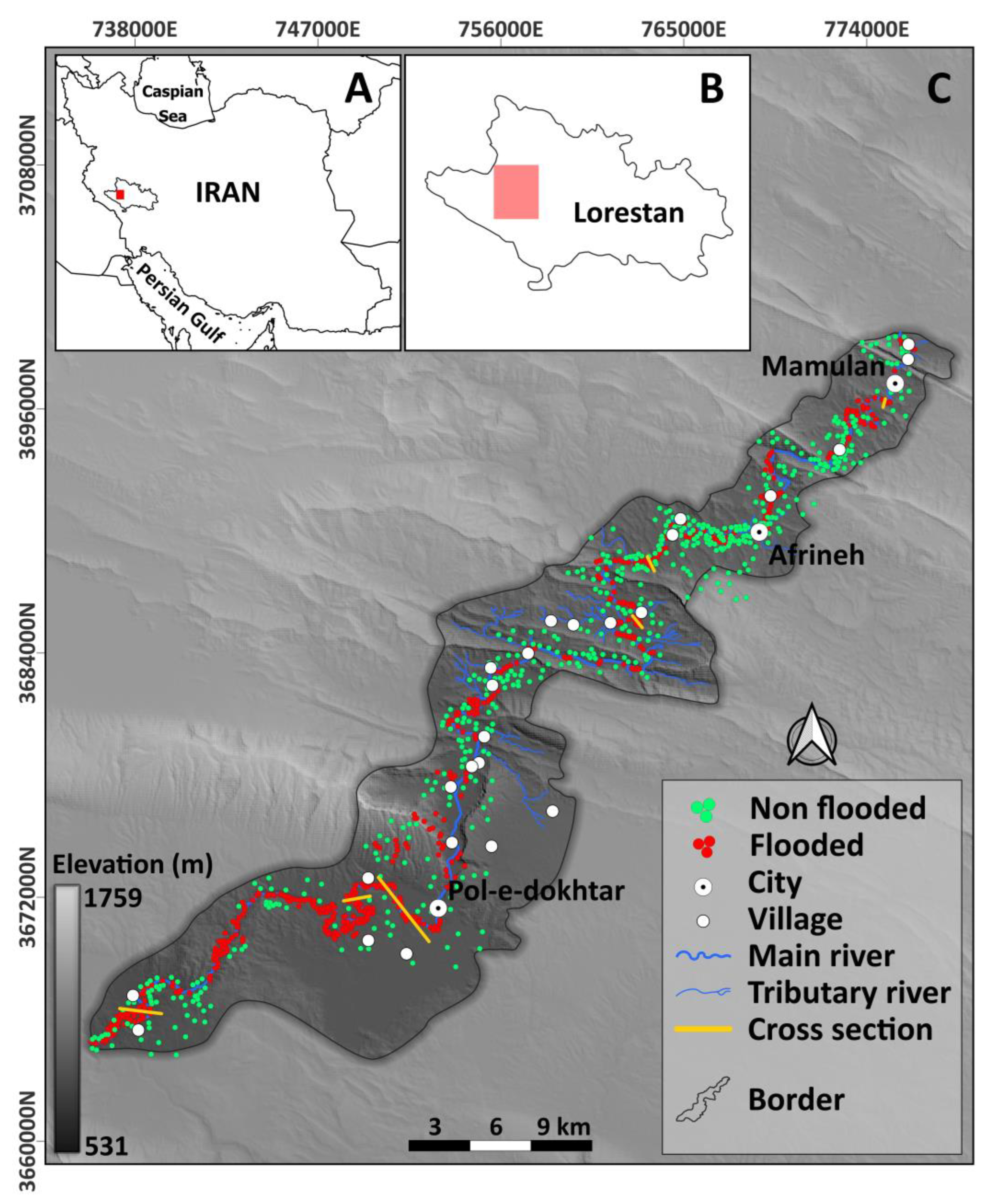
2.1. Study Area

The research encompasses approximately 100 km of the Kashkan River, situated within the Zagros folded belt in the western part of Lorestan province, Iran (Figure 1). According to the hydrological classification of Iran, the Kashkan River basin is a subset of the Persian Gulf catchment area and serves as one of the primary water tributaries to the Karkheh River [34]. This region is susceptible to heavy flooding due to the presence of numerous intermittent and ephemeral streams that discharge into the Kashkan River during precipitation events [35]. Over the past five decades, the Kashkan River has encountered 16 flooding incidents with discharges exceeding 1000 m³ s⁻¹. The most significant flooding event occurred in 2019 with a peak discharge of 4600 m³ s⁻¹. This flood, which was the highest recorded in the last century, resulted in significant damage to the urban and rural areas along the Kashkan River [36]. The intense rainfall that caused flooding in our study area began on March 25, and continued until March 29. During this period of heavy rain, the city of Pol-e-dokhtar experienced a significant amount of rainfall, with 108 mm falling on March 25. Moreover, the city of Mamulan was greatly affected by this flooding, although other cities in Lorestan Province, such as Khoramabad and Doroud, were also impacted by the flood. Notable cities within the study area include Mamulan, Afrineh, and Pol-e-dokhtar, with a total of 25 villages along the Kashkan river.

The climate in the study area leads to hot summers and cold winters, with an average annual precipitation ranging from 400 to 900 mm. Precipitation in this region encompasses both rainfall and snowfall, and winter represents the season with the highest levels of precipitation. The Kashkan River basin is characterized by a mountainous terrain, with elevations ranging from 531 to 1759 m within the study area, as determined from the SRTM Digital Elevation Model (DEM) dataset (Figure 1).

2.2. Random Forest (RF)

To identify flood-prone areas along the Kashkan River, we employed the RF algorithm implemented in the R programming language. RF is an innovative ensemble method consisting of classification and/or regression trees, which relies on the bootstrapping subset selection technique [37]. In this study, the choice of RF over other machine learning methods is made for several reasons. Firstly, RF is capable of handling complicated relationships within data. Additionally, it can handle a combination of continuous and categorical features, yielding clear and interpretable results. Another vital aspect of RF is its robustness to over-fitting, which is especially important when dealing with limited-data scenarios. This technique involves constructing models or trees using random subsets of observations and a set of controlling predictors to capture patterns within the provided data and achieve an optimal prediction performance. The RF model includes two key parameters that require optimization: the number of variables considered (mtry) and the number of trees (ntree) [38]. For this study, we set these parameters to 3 for mtry and 700 for ntree.

To ensure a reliable model performance, a meaningful split is typically determined by computing the prediction error on a subset of observations that are not included in the training process. This subset, referred to as “out-of-bag” (OOB), encompasses approximately one-third of the testing data and is selected through bootstrapping, a process involving random sampling with replacement.

2.2.1. Flood Conditioning Factors

Within our investigation, we utilized nine distinct factors, namely aspect, slope, geomorphons, plan curvature, profile curvature, terrain roughness index, surface texture, topographic wetness index (TWI), and elevation, to identify areas along the river that are susceptible to flooding (Figure 2). Our study focused specifically on topographical/morphological indexes and the correlation between topography and inundation, shedding light on the relationship between these variables. To generate and manipulate the raster layers for each factor, we utilized the SRTM Digital Elevation Model (DEM) with a spatial resolution of 30 m, SAGAGIS and QGIS software. Furthermore, all raster layers were projected onto the UTM zone 38N projection system to ensure a consistent spatial reference. Overall, factor selection depends on the characteristics of the study area and the aim of the study [4,39].

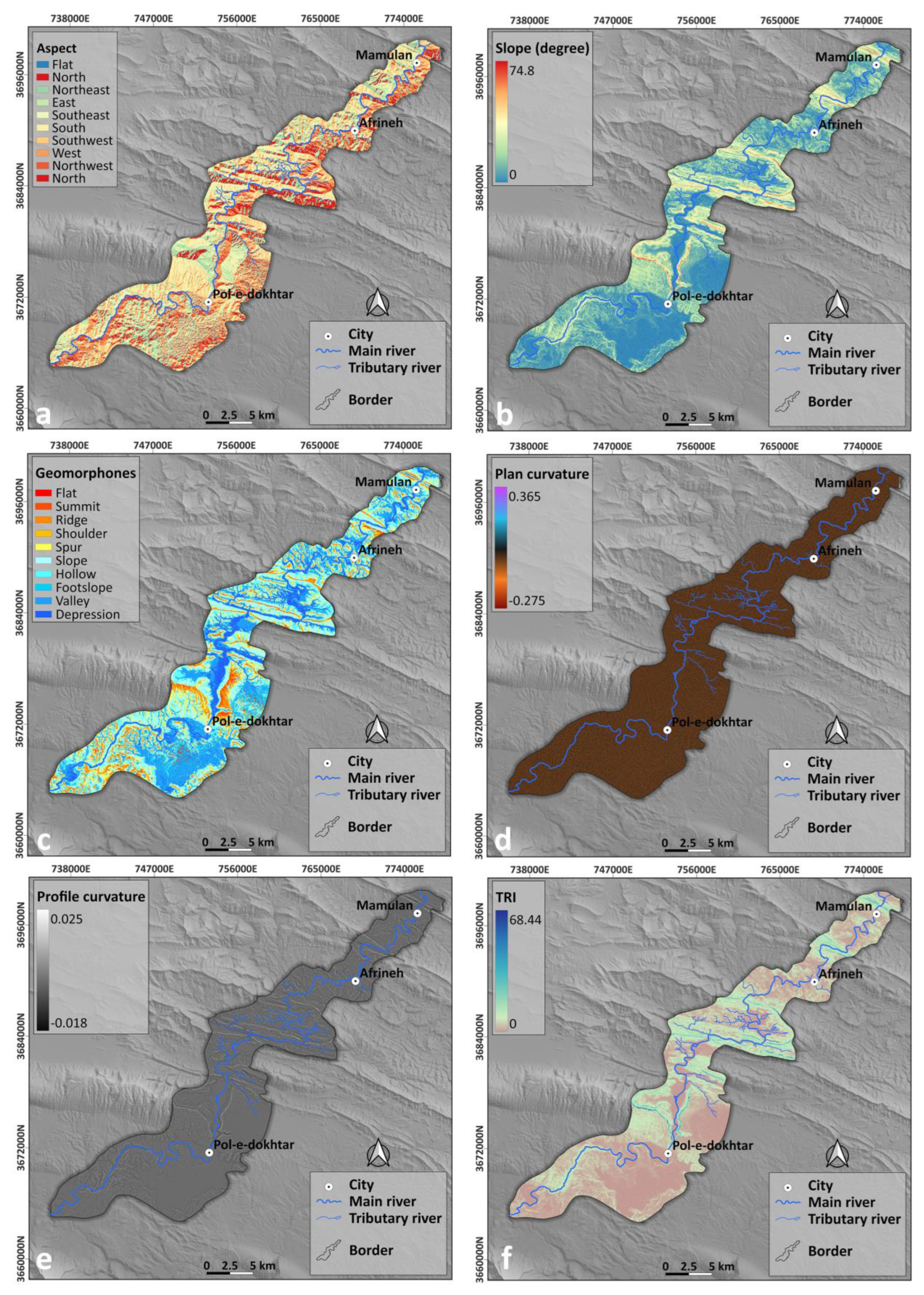
• The aspect plays a crucial role in flood mapping as it indicates the direction of each pixel in relation to a unit degree [13]. By considering the aspect map, which encompasses eight directions (N, NE, E, SE, S, SW, W, NW), we can determine the slope direction for more precise decision-making (Figure 2a). Each pixel within the aspect map is assigned a value ranging from −1 to 360, representing the specific direction it faces. The number −1 is commonly employed to represent flat or undetermined regions lacking a distinct slope direction. Such areas might encompass depressions, hollows, or flat terrains where identifying a sole slope direction is not feasible.
• The slope of an area plays a significant role in influencing the speed of drainage and the duration it takes for inundation to occur. Areas with flat or low slopes tend to be more susceptible to inundation, as water accumulates and drains at a slower pace. On the other hand, regions characterized by steep slopes facilitate rapid water drainage and the occurrence of high-velocity flows. In our present study, we employed the degree measurement to calculate the slope using a Digital Elevation Model (DEM) specific to the study area (Figure 2b).
• The geomorphon method is a relatively new approach for classifying surface landforms. It relies on pattern recognition principles and was developed by Jasiewicz and Stepinski [40]. This method utilizes a DEM as its input. It examines the elevation of a specific cell in the DEM and compares it with the surrounding cells in eight different directions up to a specified search radius. By employing a three-part pattern, the geomorphon method describes the type of landform at a given cell location [41] (Figure 2c). Geomorphons can be useful in identifying flood-prone areas due to their ability to characterize surface landforms. The landform information is valuable for assessing the topography of an area and understanding how water flows across the landscape. For instance, low-lying areas with gentle slopes and depressions can indicate potential floodplains. By analyzing the distribution and characteristics of different landforms, flood-prone regions can be identified more effectively.
• Plan curvature, also referred to as surface curvature, describes the divergence or convergence of flow patterns within a given geographical region [40]. The plan curvature provides valuable insights into the behavior of water flows and helps the algorithms to identify flood-prone areas more efficiently (Figure 2d). A plan curvature with a positive value shows that the surface is curving outwards at that cell, appearing convex from the side. Conversely, a negative value indicates that the surface is curving inwards, appearing concave from the side. A value of zero signifies that the surface is linear.
• The profile curvature metric quantifies the slope gradients along the maximum slope direction. Negative values signify a convex slope, indicating the outward curvature, whereas positive values denote a concave slope, indicating the inward curvature. A cell with a profile curvature of zero suggests a linear slope, lacking any curvature. Figure 2e shows the profile curvature of the studied area.
• The Terrain Roughness Index (TRI) is a quantitative measure that characterizes the variation in elevation between neighboring cells in a DEM (Figure 2f). This metric serves as a morphological indicator with significant relevance to the occurrence and behavior of flood events [41,42].
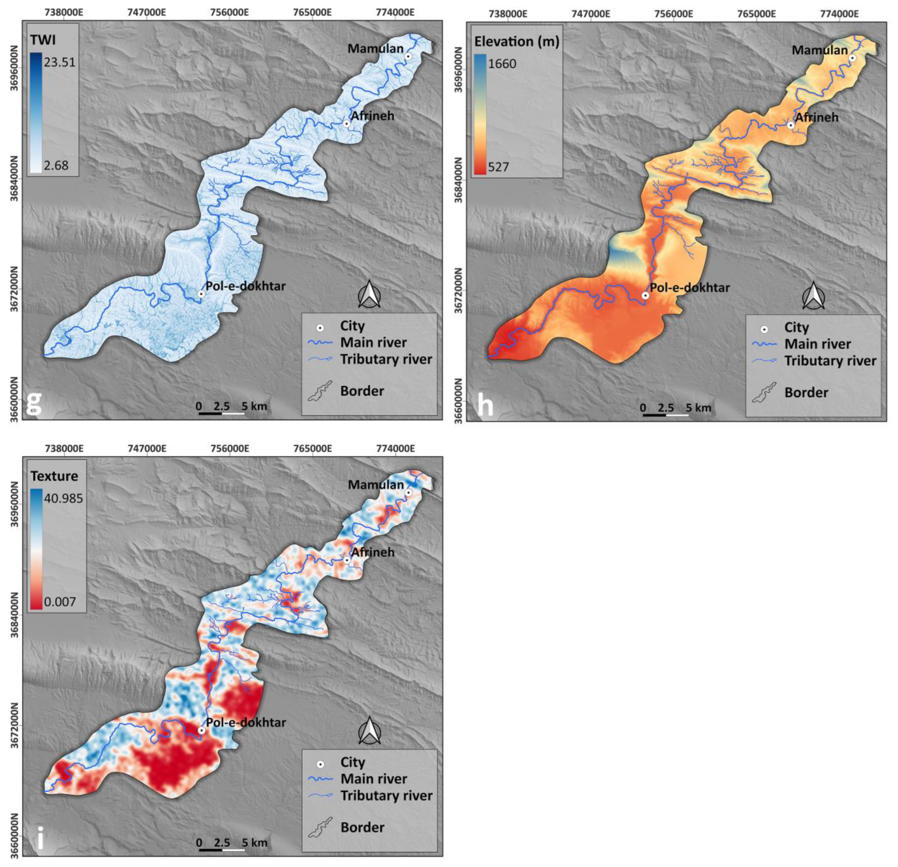
• In order to assess the topographic influences on hydrological processes [43], we employed the topographic Wetness Index (TWI). The TWI serves as a quantitative measure to capture the impact of topography on water flow (Figure 2g). Generally, higher TWI values are indicative of areas prone to flooding.
• Flooding susceptibility is significantly influenced by elevation [44]. Generally, regions situated at lower elevations are more susceptible to flooding in comparison to more elevated areas. In our study, the Shuttle Radar Topography Mission (SRTM) digital elevation model was utilized as the raster layer to represent elevation data (Figure 2h).
• The Surface Texture Index serves as a quantitative metric to depict the roughness or variation of a DEM surface. This index enables the representation of spatial variability across the terrain and is particularly advantageous for analyzing topographic features at different scales (Figure 2i).

2.2.2. Training Data Collection

The accuracy of RF output maps is heavily contingent upon the composition and caliber of the training samples employed. Particularly in the context of mapping flood-prone areas, the efficacy of both the testing and training datasets wields a substantial influence over the dependability of the resultant outcomes. Thus, underscored by its critical significance, this phase emerges as a pivotal determinant in the entire process.

In this research, a total of 1100 sample points were collected, with an equal distribution between areas affected by flooding and those that were not. This resulted in 550 samples being attributed to flooded areas (with an assigned value of 1), and an additional 550 samples assigned to non-flooded regions (with an assigned value of 0), which were overlaid with the nine flood conditioning factors. The collection process involved visually inspecting true color compositions derived from Landsat 8 OLI and Sentinel-2 optical imagery, and utilizing the NDWI raster layer derived from these satellite images. NDWI was calculated using the blue and short-wave infrared (SWIR) bands of Landsat 8 OLI (bands 2 and 6) and Sentinel-2 (bands 2 and 11) satellite imageries. These images were specifically associated with the flooding event that occurred in March 2019. Out of the entire set of collected samples, 75% were designated for training purposes, while the remaining 25% were allocated for testing. Figure 1 shows the distribution of flooded and non-flooded sample points across the study area.

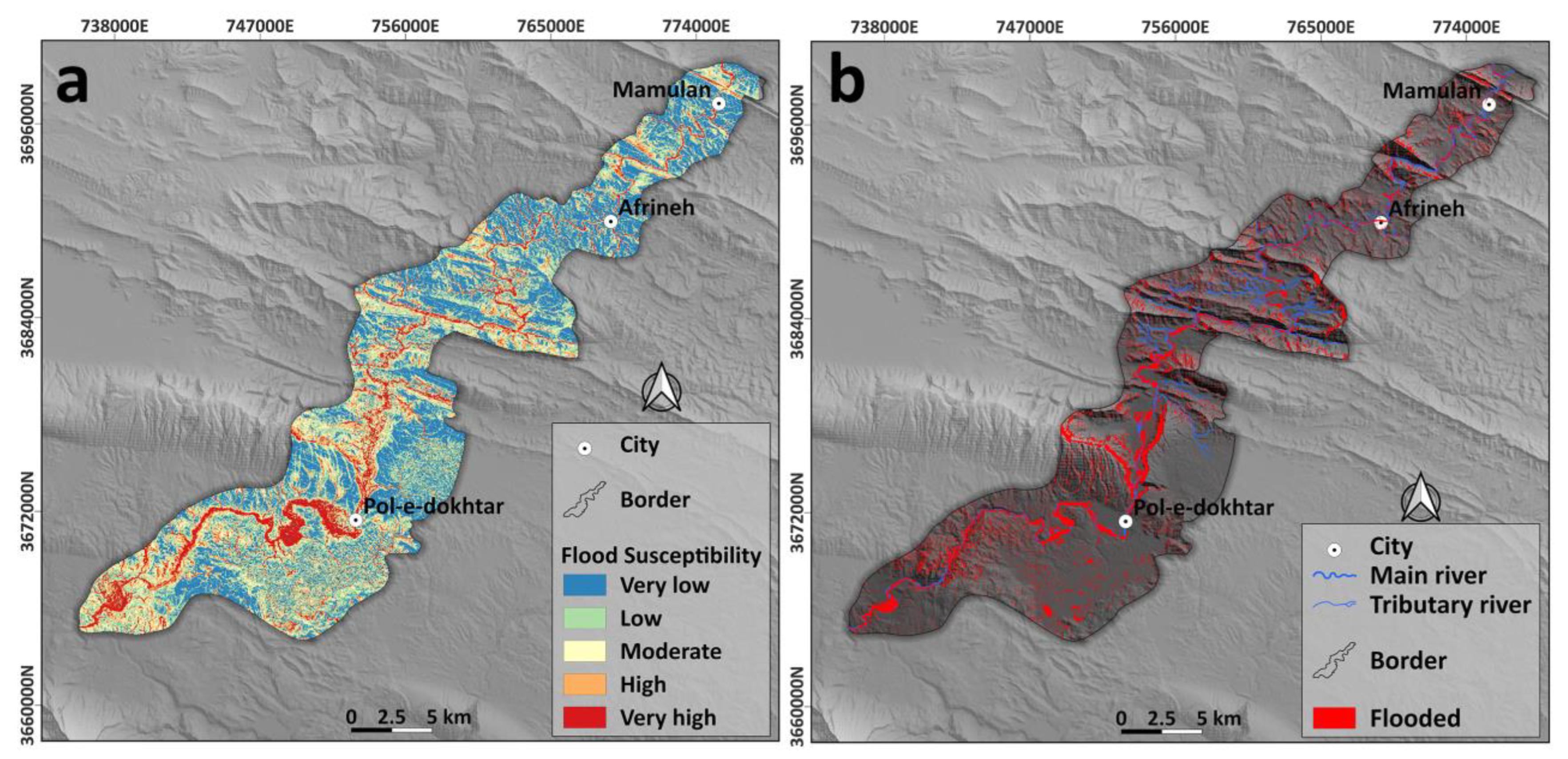
2.2.3. Flood Map Generation

After generating a flood susceptibility map using an RF algorithm, we proceeded to categorize the output map into five distinct classes: very low (0–0.15), low (0.16–0.31), moderate (0.32–0.5), high (0.51–0.73) and very high (0.74–1) susceptibility levels (Figure 3a). This classification was achieved through the application of the natural break method, a statistical approach commonly employed in numerous flood mapping studies involving RF [4,11,17]. The natural break method serves as a valuable tool for data classification, especially within the context of flood mapping. It functions by discerning inherent patterns and breakpoints within the data distribution, effectively grouping the flood map data into meaningful categories. Given the dynamic nature of flood maps, which often exhibit varying intensities and extents, the natural break method is adept at accurately capturing these fluctuations. Additionally, the natural break method plays a pivotal role in minimizing the variance within each class while simultaneously maximizing the variance between classes. This dual effect contributes to the creation of well-defined, clearly distinguishable categories. Such precision is crucial to the meaningful interpretation of flood severity, enhancing the overall significance of the results.

2.3. Validation and Accuracy Assessment

Validation and accuracy assessment play a crucial role in the modeling of natural phenomena [42]. In this study, we employed SAR-based flood/inundation maps to validate our flood-prone map generated through the RF technique. By utilizing SAR-based flood maps, we were able to observe actual instances of flooding and identify the specific areas that experienced flooding during a real flood event. This enabled us to assess whether the RF method accurately identified the areas prone to flooding along the Kashkan River. To accomplish this, we utilized Sentinel-1 SAR imagery from the flooding events in March 2019 and the SNAP software. To extract the flooded/inundated areas from the SAR imagery, we applied the OTSU thresholding method [43], which is widely used for this purpose. The Otsu thresholding algorithm is capable of automatically determining an optimal threshold by maximizing the variance between different classes and minimizing the variance within each class. It has been proven to be a straightforward and effective technique for mapping surface water, even in challenging scenarios involving complex water bodies such as areas with submerged vegetation, sedimented water, and turbid water.

To evaluate the effectiveness and reliability of our RF map for identifying flood-prone areas, we utilized the Area Under the Curve (AUC), sensitivity, and specificity. These metrics are frequently employed to assess the model’s ability to accurately classify distinct classes. AUC is widely employed in natural hazard investigations due to its comprehensive nature and ability to produce meaningful and easily interpretable results [44]. The AUC method generates a value ranging from zero to one, with a value of one indicating 100% success. Therefore, the closer the AUC value is to one, the higher the accuracy of the technique in question. In general, the AUC provides a single number that quantifies the overall performance of the model across different threshold values. Sensitivity, also known as true positive rate (TPR), measures the proportion of actual positive cases that are correctly identified by the model. High sensitivity indicates that the model is effective at correctly identifying positive cases. Specificity or true negative rate (TNR) measures the proportion of actual negative cases that are correctly identified by the model. High specificity indicates that the model is effective at correctly identifying negative cases.

Table 1. Values of AUC, sensitivity, and specificity.

Parameter	Value
AUC	0.8656
Sensitivity	0.9236
Specificity	0.9

displays the values for Area Under the Curve (AUC), sensitivity, and specificity.

3. Results

In this study, we employed the random forest machine learning algorithm to detect areas prone to flooding along the Kashkan river in the Zagros Mountain range. Additionally, we examined the influence of morphology/topography on the occurrence of flooding and inundation specifically at the meander locations along the river. Figure 3a illustrates the flood-prone areas determined by the RF algorithm, while Figure 3b displays the flooded/inundated areas identified through Sentinel-1 SAR imagery during the March 2019 flooding event. According to Figure 3a, the RF map’s “very high” and “high” susceptible flood areas significantly align with the flooded/inundated regions depicted in Figure 3b. The majority of flood-prone areas are concentrated along the primary course of the Kashkan river and around the meander locations, as observed in Figure 3. Moreover, the southern regions of the study area exhibit a larger extent of “very high” and “high” flood-prone classes compared to the northern regions. Figure 3 also reveals that meanders near Pol-e-dokhtar city encompass substantial areas classified as “very high” and “high” flood-prone. Conversely, “moderate”, “low”, and “very low” flood-prone areas are predominantly found in more distant regions from the river, primarily in mountainous areas and higher elevations.

The importance of each factor influencing flooding is displayed in

Table 2. Importance of flood conditioning factors using RF method.

Conditioning Factor	Mean Decrease Accuracy
Aspect	22.41
Slope	20.67
Geomorphons	47.90
Plan Curvature	1.41
Profile Curvature	23.24
TRI	25.45
Texture	26.97
TWI	71.36
Elevation	79.49

using a measure called Mean Decrease Accuracy. This method helps us to evaluate the importance of features based on how much they contribute to the overall accuracy of the model. Essentially, it reveals the factors with the greatest impact on the model’s predictions. The results from the mean decrease accuracy indicate that elevation (79.49), TWI (71.36), and Geomorphons (47.90) hold the highest importance in our study area for predicting flood-prone areas. Following this, surface texture (26.97), TRI (25.45), profile curvature (23.24), aspect (22.41), slope (20.67), and plan curvature (1.41) exhibit the next level of importance in our study area. Understanding the importance of each factor can offer valuable insights for decision-makers, aiding them in making more effective flood management choices and reducing flood-related damage. Moreover, researchers can utilize this information to gain a better grasp of how the physical characteristics of the landscape, like its morphology, relate to the flooding of riverbanks.

In the March 2019 flooding event, a total of 63.02 km² experienced flooding/inundation according to the SAR-based flood map (

Table 3. Areas of flooded/inundated regions of March 2019 flooding event and the different classes of the RF flood susceptibility map.

Class	Area km2
Flooded/inundated (SAR)	63.02
Very high (RF)	31.3
High (RF)	43.2
Moderate (RF)	62.59
Low (RF)	85.88
Very low (RF)	123.61
Total area of the study area	346.58

). The RF flood susceptibility map analysis reveals that, within the study area, 31.3 km² fall under the category of “very high” flood susceptibility, while 43.2 km² are classified as having “high” susceptibility. The combined area of the “very high” and “high” susceptibility classes in the RF map corresponds to the extent of the flooded/inundated regions identified through SAR imagery, as illustrated in Figure 3. Furthermore, the analysis indicates that the “moderate”, “low”, and “very low” susceptible regions encompass areas measuring 62.59, 85.88, and 123.58 km², respectively.

Figure 4 illustrates the location of the first cross-section and depicts the extent of the flooding event in 2019 (Figure 4b). It also displays the regions classified as “very high” and “high” flood susceptibility on the profile (Figure 4c). At the first cross-section, the flood covered a larger expanse on the outer bank of the meander, while a smaller portion of the inner bank was inundated. The outer bank exhibits a greater coverage of the “very high” susceptible class compared to the inner bank. In contrast, the outer bank has a smaller area covered by the “high” susceptible class compared to the inner bank. Upon observing Figure 4c, it becomes evident that surface slope of the “very high” category demonstrates a smoother gradient on the outer bank, whereas the same category on the inner bank possesses a steeper slope. Consequently, the “very high” category encompasses a larger area of the outer bank than the inner bank, which aligns with the flooded area during the 2019 flooding event. Additionally, the “high” susceptible class on the outer bank displays a steeper slope than the inner bank. This class covers a smaller area of the outer bank but exhibits a larger coverage of the inner bank.

In the second cross-section, similar to the first one, the outer bank experienced extensive flooding in comparison to the inner bank. Despite the main river channel being closer to the inner banks, the wider space and gentler slope on the outer bank allowed for the floodwaters to cover a larger area. Figure 5c further demonstrates that the outer bank has a significantly larger region classified as having “very high” flood susceptibility compared to the inner bank. According to Figure 5, during the 2019 flooding event, the flood reached the “high” susceptible class on the outer bank, whereas it did not reach the maximum elevation of the “very high” flood susceptible class on the inner bank.

Figure 6 illustrates the third cross-section within the study area. In this cross-section, the inner bank has a greater extent of flooding/inundation compared to the outer bank; however, the flood flow on the outer bank reached a higher level (Figure 6c). In this specific cross-section, both the inner and outer banks experienced flooding in the area designated as having a “very high” flood susceptibility. The outer bank of the valley has a steep slope, while the inner bank has relatively gentler slopes. On the outer bank, the “high” flood susceptibility class covers a smaller area, whereas at the inner bank of the meanders, the “high” class has a larger coverage. As shown in Figure 6c, the flood flow inundated significant portions of the “high” class on the inner bank, surpassing the coverage on the outer bank.

According to Figure 7b, similar to the previous cross-section, the inner bank of the meander experienced more extensive flooding. The RF map (Figure 7a) also illustrates that a larger portion of the inner bank is categorized as having “very high” susceptibility to floods, in contrast to the outer bank. Figure 7c demonstrates that the inner bank possesses a gentler slope and topography, whereas the outer bank exhibits a steep and abrupt slope. Interestingly, the maximum boundary of the “very high” category and the maximum extent of the flooded area during the 2019 flooding event coincide and align with each other. Additionally, the “high” category covers a larger area of the inner bank of the meander compared to the outer bank.

Figure 8 shows a long profile covering three significant meanders. It demonstrates that the floodplain where the city of Pol-e-dokhtar is situated is highly prone to flooding, as a substantial portion of land along this profile falls into the categories of “very high” and “high” susceptibility to flooding. Additionally, Figure 8b illustrates that the inner banks of the meanders were flooded during the flooding event in March 2019. The RF map (Figure 8a) indicates that a considerable portion of the floodplain is in the “very high” and “high” flood susceptibility classes, while the right side of the cross-section, where the first meander is located, displays a small area classified as “highly” susceptible to flooding. Conversely, the larger area on the right side of the profile falls into the “high” susceptibility class due to its gentler slope and smoother topography.

Utilizing the RF algorithm, the inner bank of the fifth cross-section was categorized as having ‘very high’ and ‘high’ susceptibility to flooding, as depicted in Figure 9a. By comparing this classification with the flooded areas shown in Figure 9b, it becomes evident that the algorithm accurately identified the flood-prone areas and correctly categorized them as having “very high” and “high” susceptibility to floods, as they correspond to the flooded areas during the 2019 flooding event. In general, the inner bank of this cross-section can be characterized by its gentle slope, while the outer bank exhibits a steep slope adjacent to the river channel. The “very high” class on the outer bank could extend to higher elevations compared to the inner bank. Conversely, on the inner bank, the same class covers a larger area.

4. Discussion

4.1. Model Capability to Identify Flood-Prone Areas

This study utilized topographical/morphological data extracted from the DEM of the study area with a 30 m resolution, as well as the RF machine learning algorithm, to identify flood-prone areas along the Kashkan river. To verify the accuracy of the flood susceptibility map generated by the random forest algorithm, Sentinel-1 SAR imagery and the OTSU thresholding method were employed to extract flooded areas during a specific flooding event that occurred in the study area in March 2019.

A visual comparison of the RF susceptibility map and the SAR-based flood map revealed a strong correlation, indicating the model’s accuracy in classifying flood-prone areas (Figure 3). Specifically, the “very high” and “high” flood susceptibility categories identified by the RF algorithm corresponded to the regions that experienced flooding during the 2019 flooding event (Figure 3). This demonstrates the effectiveness of the model in accurately identifying areas at high risk of flooding. Moreover, the results of the study shed light on the importance of topographical and morphological factors in determining flood-prone areas using machine learning algorithms, such as RF. By considering the topography and morphology of the study area, the RF model successfully identified the meandering banks as the primary locations prone to flooding. This observation was further supported by the SAR map, which showed that almost all of the meander banks experienced inundation during the 2019 flooding event. The consistency between the study’s findings and the existing literature on flood-prone areas adds further credibility to the results. The fact that the RF model accurately identified and classified the areas prone to flooding aligns with previous research [45,46], strengthening the validity and reliability of the study’s conclusions.

Examining ‘very high’ and ‘high’ flood-prone regions along cross-sections revealed distinct variations in maximum elevation on the outer and inner sides of the meander. When investigating flood-prone areas, it is crucial to consider that the model identifies these areas independently of potential flood flow elevations and regardless of their position as outer or inner sides of the meander. As a result, the model determined flood-prone areas based on the given morphological and topographical data. Consequently, this implies that the highlighted areas may have either “very high” or “high” susceptibility to flooding/inundation. Across all cross-sections, the inundated areas during the March 2019 flooding event exhibited higher elevations on one side of the meander compared to the other side. This occurrence can be partly attributed to the SAR images classifying wet areas as flooded. During flooding, saturated ground due to rainfall may be mistakenly considered flooded/inundated in the SAR image, despite not experiencing actual flooding. Additionally, the accuracy of the DEM is crucial to ensure that the flooded areas precisely align with the correct elevation. Studies indicate that the SRTM DEM possesses a vertical accuracy of approximately ±5 m, which can vary across different regions [47,48]. Consequently, these represent the primary limitations when using SAR imagery and medium-resolution DEM in flood-prone area investigations.

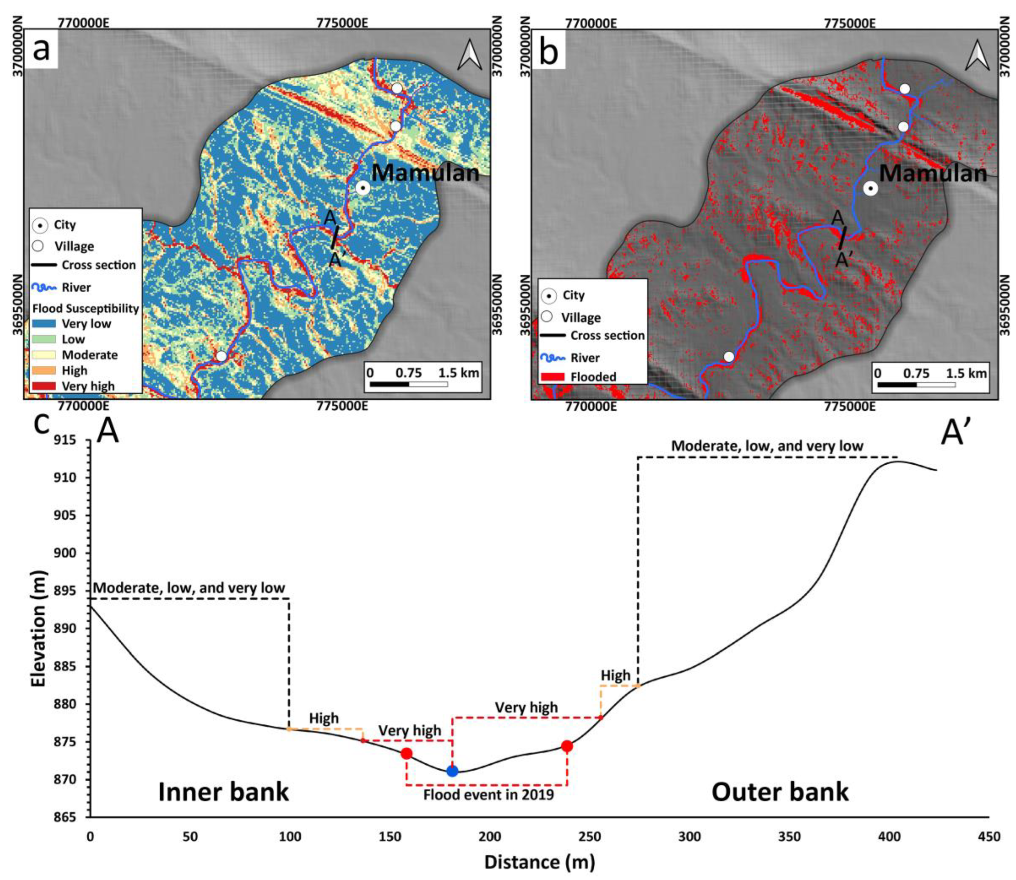
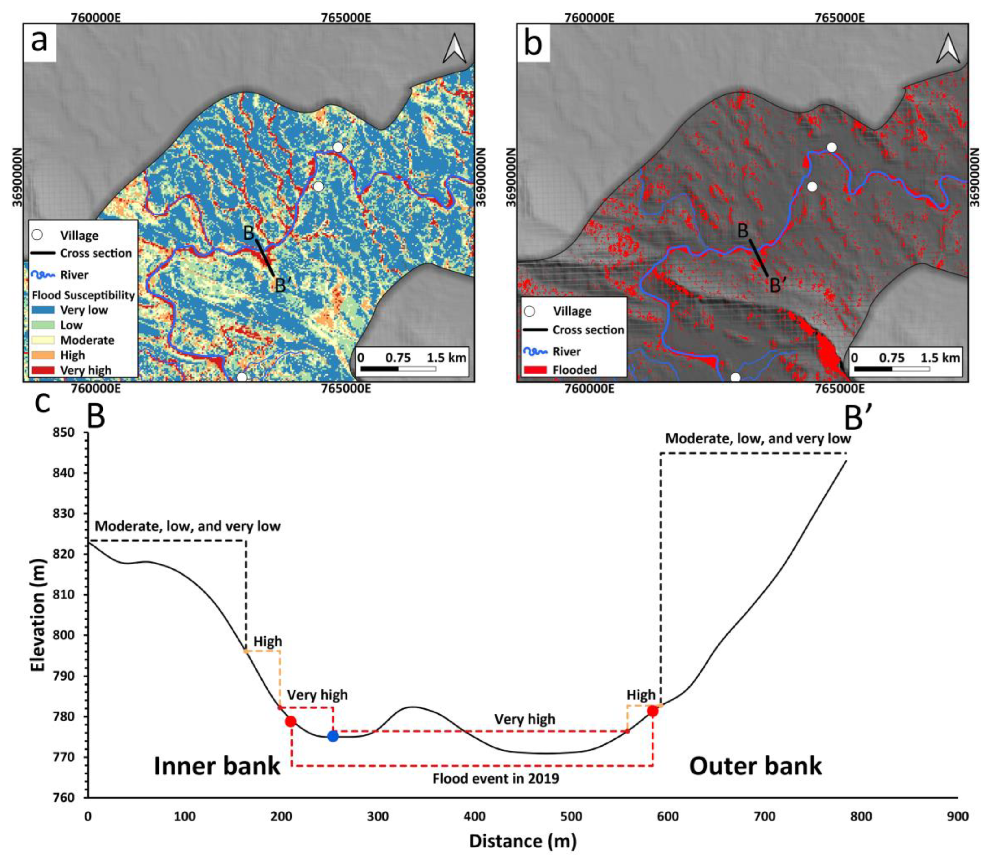
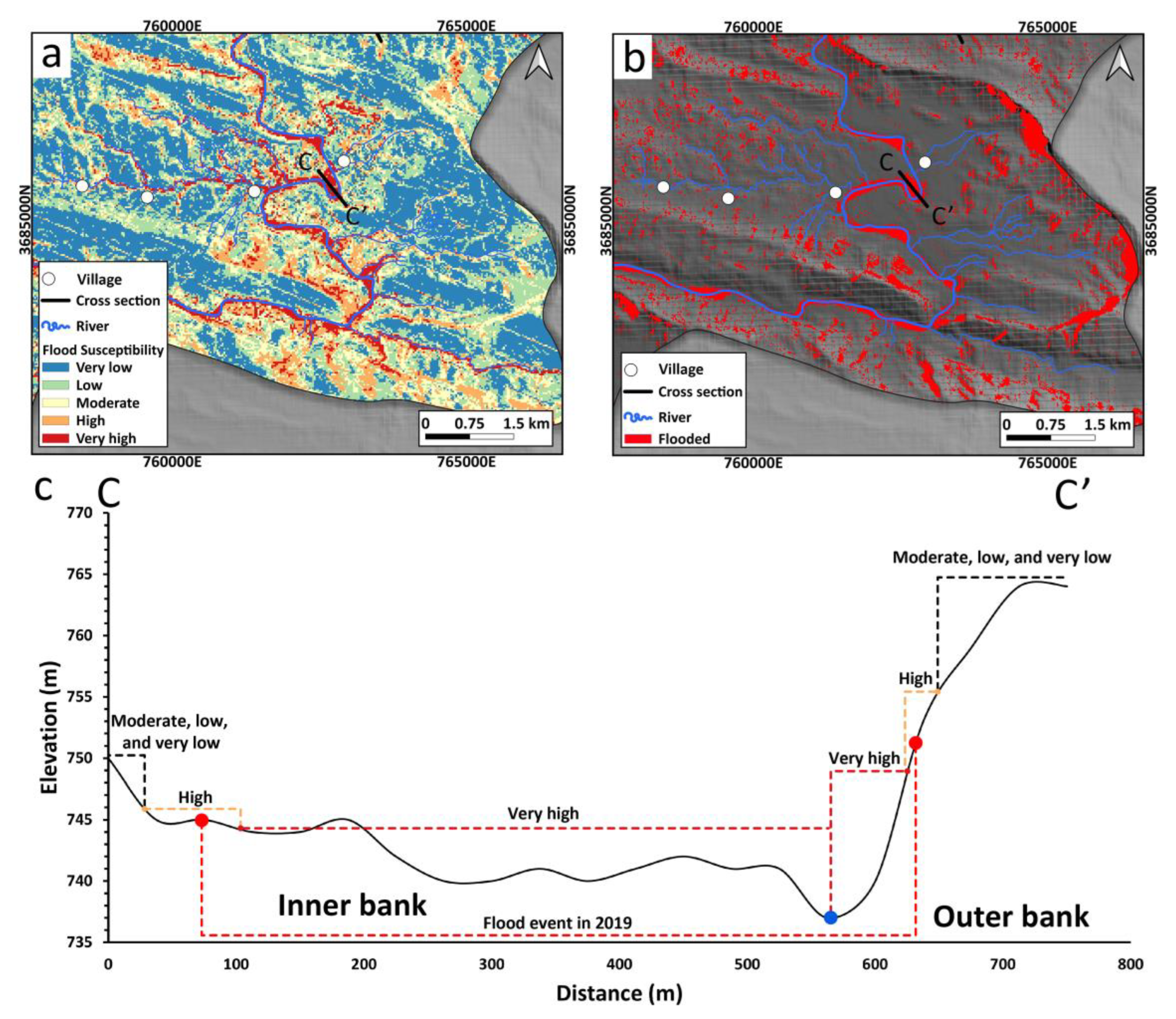
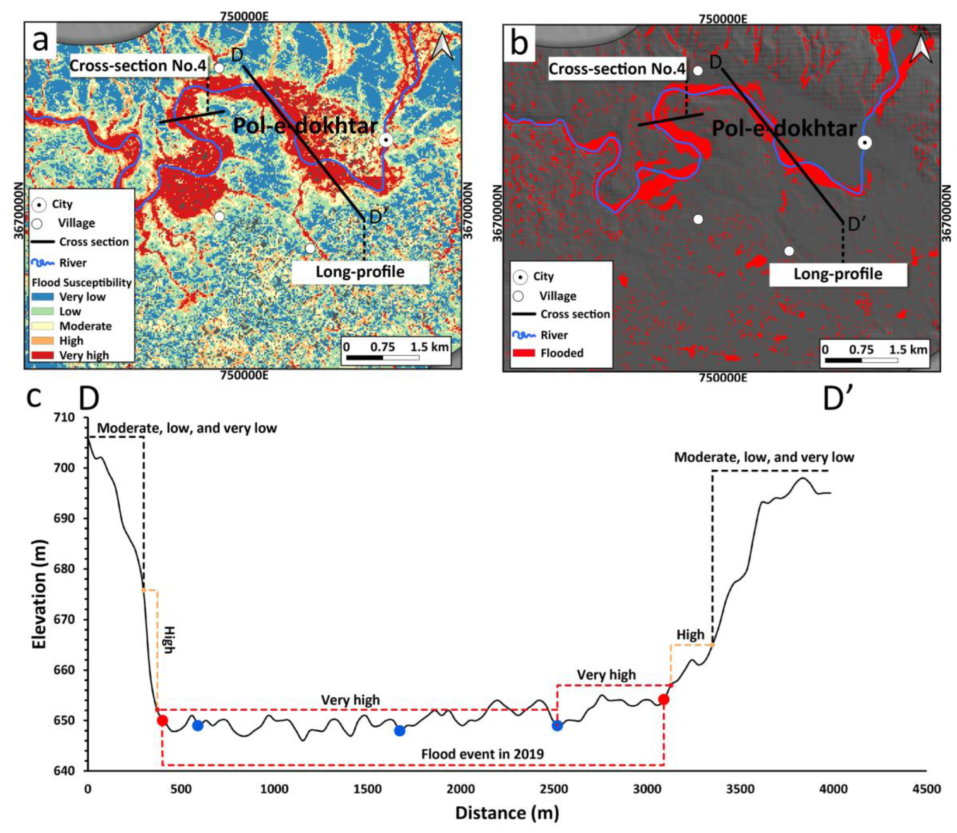
4.2. Impact of Topography on Inundation

The inundation of meander banks, whether inner or outer, is influenced by various factors, including flow velocity, meander sinuosity and channel roughness. This study specifically focused on investigating how topography affects the flooding of inner and outer banks in the Kashan River. Regardless of the river’s hydrological characteristics, the findings revealed that topographical confinement plays a significant role in the inundation of meander banks. By analyzing cross-sections, it was observed that when a meander is laterally confined, the unconfined side is more susceptible to flooding. However, the flood flow may be substantially higher in the confined bank, likely due to the flow velocity and discharge volume during flooding events. The study results demonstrated that the smoother relief on the inner banks makes them more prone to inundation during floods. This factor is important because, during flooding, the smooth relief and unconfined topography provide suitable space for the flood to overflow. The unconfined topography also assists in reducing the flow elevation on the confined opposite bank. Consequently, it can be concluded that, compared to the topographically unconfined inner banks, the outer banks are less susceptible to flooding. However, if the outer bank offers a smoother relief and space for overflow, as depicted in Figure 4c, it becomes the most flood-prone area compared to the inner banks. Therefore, topographical confinement primarily determines inundation, regardless of the river’s hydrological characteristics. The analysis of the RF flood susceptibility map and SAR-based flood map revealed that the inner banks of the Kashkan River are more susceptible to flooding compared to the outer banks. This can primarily be attributed to the smoother relief and unconfined topography of the inner banks in contrast to the outer banks.

The analysis of the cross-sections revealed that investigating the role of topography and morphology depends on the scale of the landforms. For instance, when studying small-scale landforms like point bars or channel bed morphology, a high-resolution DEM is necessary. On the other hand, for large-scale landforms like flood plains and major terraces, the 30 m DEM suffices. The study’s findings indicated that, during floods, the slopes along the river also experienced inundation. This can be attributed to the overall valley cross-section; a wider and deeper cross-section allows for water to spread out, reducing flow velocities and minimizing erosive forces that contribute to flooding. Conversely, a narrow and shallow cross-section results in higher flow velocities and elevated water levels, eventually leading to inundation of the slopes.

It is worth emphasizing that while there are numerous factors that govern flooding and inundation in meandering rivers, the primary focus of this study was twofold. Firstly, it aimed to identify the areas along the Kashkan River that are susceptible to flooding by employing a precise methodology and utilizing topographical data. Secondly, the study sought to examine the influence of topography on inundation in a meandering river.

Overall, this study demonstrated that employing the RF model and utilizing morphological data can offer a rapid and dependable approach to identifying flood-prone areas along a mountainous meandering river. However, certain limitations, particularly those related to the vertical and spatial accuracy of the DEM, were observed. Despite these limitations, the method proved to be highly valuable in regions lacking sufficient measured data and in remote areas. The RF flood susceptibility map generated from this approach can be a valuable tool for decision-makers to implement effective measures in mitigating the damage caused by future floods.

5. Conclusions

Flooding is an increasingly prevalent natural hazard at a global scale. Therefore, it is crucial to identify areas that are prone to flooding to mitigate future flood damage. The Kashkan river, located in the Zagros Mountain range in western Iran, experiences significant flooding annually. The findings of this study demonstrated that by utilizing topographical data and employing the RF machine learning algorithm, flood-prone areas along the Kashkan river can be accurately identified. Moreover, the study revealed that the topographical confinement of the river’s meanders significantly influences the inundation of the inner and outer banks. In the majority of cases in the Kashkan river, the inner banks exhibit a higher susceptibility to flooding compared to the outer banks. This can be primarily attributed to the smoother relief, which allows for suitable overflow space, as well as the unconfined topography of the inner banks.

References

1. Lazzarin, T.; Defina, A.; Viero, D.P. Assessing 40 Years of Flood Risk Evolution at the Micro-Scale Using an Innovative Modeling Approach: The Effects of Urbanization and Land Planning. Geosciences 2023, 13, 112. [Google Scholar] [CrossRef]
2. Arnell, N.W.; Gosling, S.N. The impacts of climate change on river flood risk at the global scale. Clim. Chang. 2016, 134, 387–401. [Google Scholar] [CrossRef]
3. Ha, J.; Kang, J.E. Assessment of flood-risk areas using random forest techniques: Busan Metropolitan City. Nat. Hazards 2022, 111, 2407–2429. [Google Scholar] [CrossRef]
4. Esfandiari, M.; Abdi, G.; Jabari, S.; McGrath, H.; Coleman, D. Flood Hazard Risk Mapping Using a Pseudo Supervised Random Forest. Remote Sens. 2020, 12, 3206. [Google Scholar] [CrossRef]
5. Khosravi, K.; Panahi, M.; Golkarian, A.; Keesstra, S.D.; Saco, P.M.; Bui, D.T.; Lee, S. Convolutional neural network approach for spatial prediction of flood hazard at national scale of Iran. J. Hydrol. 2020, 591, 125552. [Google Scholar] [CrossRef]
6. Amitrano, D.; Di Martino, G.; Iodice, A.; Riccio, D.; Ruello, G. Unsupervised rapid flood mapping using Sentinel-1 GRD SAR images. IEEE Trans. Geosci. Remote Sens. 2018, 56, 3290–3299. [Google Scholar] [CrossRef]
7. CEOS. The Use of Earth Observing Satellites for Hazard Support: Assessments & Scenarios. 2018. Available online: http://drm.cenn.org/Trainings/Multi%20Hazard%20Risk%20Assessment/Lectures_ENG/Session%2002%20Spatial%20data%20requirements%20for%20risk%20assessment/background/CEOS_DMSG_Final_Hazards_Report10_02.pdf (accessed on 20 June 2023).
8. Ghahraman, K.; Nagy, B. Flood risk on arid alluvial fans: A case study in the Joghatay Mountains, Northeast Iran. J. Mt. Sci. 2023, 20, 1183–1200. [Google Scholar] [CrossRef]
9. Khosravi, K.; Pourghasemi, H.R.; Chapi, K.; Bahri, M. Flash flood susceptibility analysis and its mapping using different bivariate models in Iran: A comparison between Shannon’s entropy, statistical index, and weighting factor models. Environ. Monit. Assess. 2016, 188, 656. [Google Scholar] [CrossRef]
10. Feng, Q.; Gong, J.; Liu, J.; Li, Y. Flood Mapping Based on Multiple Endmember Spectral Mixture Analysis and Random Forest Classifier—The Case of Yuyao, China. Remote Sens. 2015, 7, 12539–12562. [Google Scholar] [CrossRef]
11. Rafiei-Sardooi, E.; Azareh, A.; Choubin, B.; Mosavi, A.H.; Clague, J.J. Evaluating urban flood risk using hybrid method of TOPSIS and machine learning. Int. J. Disaster Risk Reduct. 2021, 66, 102614. [Google Scholar] [CrossRef]
12. Deroliya, P.; Ghosh, M.; Mohanty, M.P.; Ghosh, S.; Rao, K.D.; Karmakar, S. A novel flood risk mapping approach with machine learning considering geomorphic and socio-economic vulnerability dimensions. Sci. Total Environ. 2022, 851, 158002. [Google Scholar] [CrossRef] [PubMed]
13. Farhadi, H.; Najafzadeh, M. Flood risk mapping by remote sensing data and random forest technique. Water 2021, 13, 3115. [Google Scholar] [CrossRef]
14. Lee, S.; Kim, J.-C.; Jung, H.-S.; Lee, M.J.; Lee, S. Spatial prediction of flood susceptibility using random-forest and boosted-tree models in Seoul metropolitan city, Korea. Geomat. Nat. Hazards Risk 2017, 8, 1185–1203. [Google Scholar] [CrossRef]
15. Khosravi, K.; Pham, B.T.; Chapi, K.; Shirzadi, A.; Shahabi, H.; Revhaug, I.; Prakash, I.; Bui, D.T. A comparative assessment of decision trees algorithms for flash flood susceptibility modeling at Haraz watershed, northern Iran. Sci. Total Environ. 2018, 627, 744–755. [Google Scholar] [CrossRef]
16. Cao, C.; Xu, P.; Wang, Y.; Chen, J.; Zheng, L.; Niu, C. Flash flood hazard susceptibility mapping using frequency ratio and statistical index methods in coalmine subsidence areas. Sustainability 2016, 8, 948. [Google Scholar] [CrossRef]
17. Mangukiya, N.K.; Sharma, A. Flood risk mapping for the lower Narmada basin in India: A machine learning and IoT-based framework. Nat. Hazards 2022, 113, 1285–1304. [Google Scholar] [CrossRef]
18. Goffi, A.; Stroppiana, D.; Brivio, P.A.; Bordogna, G.; Boschetti, M. Towards an automated approach to map flooded areas from Sentinel-2 MSI data and soft integration of water spectral features. Int. J. Appl. Earth Obs. Geoinf. 2020, 84, 101951. [Google Scholar] [CrossRef]
19. Zhang, M.; Chen, F.; Liang, D.; Tian, B.; Yang, A. Use of Sentinel-1 GRD SAR images to delineate flood extent in Pakistan. Sustainability 2020, 12, 5784. [Google Scholar] [CrossRef]
20. Singha, M.; Dong, J.; Sarmah, S.; You, N.; Zhou, Y.; Zhang, G.; Doughty, R.; Xiao, X. Identifying floods and flood-affected paddy rice fields in Bangladesh based on Sentinel-1 imagery and Google Earth Engine. ISPRS J. Photogramm. Remote Sens. 2020, 166, 278–293. [Google Scholar] [CrossRef]
21. Twele, A.; Cao, W.; Plank, S.; Martinis, S. Sentinel-1-based flood mapping: A fully automated processing chain. Int. J. Remote Sens. 2016, 37, 2990–3004. [Google Scholar] [CrossRef]
22. Voigt, S.; Kemper, T.; Riedlinger, T.; Kiefl, R.; Scholte, K.; Mehl, H. Satellite image analysis for disaster and crisis-management support. IEEE Trans. Geosci. Remote Sens. 2007, 45, 1520–1528. [Google Scholar] [CrossRef]
23. Wang, Z.; Lai, C.; Chen, X.; Yang, B.; Zhao, S.; Bai, X. Flood hazard risk assessment model based on random forest. J. Hydrol. 2015, 527, 1130–1141. [Google Scholar] [CrossRef]
24. Rawat, S.; Saini, R.; Singh, A. Mapping of Waterlogged Areas and Silt-Affected Areas After the Flood Using the Random Forest Classifier on the Sentinel-2 Dataset. In Machine Intelligence Techniques for Data Analysis and Signal Processing: Proceedings of the 4th International Conference MISP 2022, Online, 12–14 March 2022; Springer Nature: Singapore, 2023; Volume 1. [Google Scholar]
25. Arlisa, S.D.; Handayani, H.H. Flood Vulnerability Analysis using Random Forest Method in Gresik Regency, Indonesia. In IOP Conference Series: Earth and Environmental Science; IOP Publishing: Bristol, UK, 2023. [Google Scholar]
26. Mirkazemi, S.M.; Jalalkamali, N.; Irandoost, M. Spatial Flood Forecasting Modeling under Lack of Data Using RS and Optimized Support Vector Machine: A Case Study of the Zahedan Watershed. Nat. Hazards Rev. 2023, 24, 05023005. [Google Scholar] [CrossRef]
27. Youssef, A.M.; Pradhan, B.; Dikshit, A.; Mahdi, A.M. Comparative study of convolutional neural network (CNN) and support vector machine (SVM) for flood susceptibility mapping: A case study at Ras Gharib, Red Sea, Egypt. Geocarto Int. 2022, 37, 11088–11115. [Google Scholar] [CrossRef]
28. Sarigöl, M.; Yesilyurt, S.N. Flood routing calculation with ANN, SVM, GPR, and RTE methods. Pol. J. Environ. Stud. 2022, 31, 5221–5228. [Google Scholar] [CrossRef]
29. Ghosh, A.; Dey, P.; Ghosh, T. Integration of RS-GIS with Frequency Ratio, Fuzzy Logic, Logistic Regression and Decision Tree Models for Flood Susceptibility Prediction in Lower Gangetic Plain: A Study on Malda District of West Bengal, India. J. Indian Soc. Remote Sens. 2022, 50, 1725–1745. [Google Scholar] [CrossRef]
30. Filipova, V.; Hammond, A.; Leedal, D.; Lamb, R. Prediction of flood quantiles at ungauged catchments for the contiguous USA using Artificial Neural Networks. Hydrol. Res. 2022, 53, 107–123. [Google Scholar] [CrossRef]
31. Breiman, L. Random forests. Mach. Learn. 2001, 45, 5–32. [Google Scholar] [CrossRef]
32. Feng, Q.; Liu, J.; Gong, J. UAV remote sensing for urban vegetation mapping using random forest and texture analysis. Remote Sens. 2015, 7, 1074–1094. [Google Scholar] [CrossRef]
33. Rodriguez-Galiano, V.F.; Ghimire, B.; Rogan, J.; Chica-Olmo, M.; Rigol-Sanchez, J.P. An assessment of the effectiveness of a random forest classifier for land-cover classification. ISPRS J. Photogramm. Remote Sens. 2012, 67, 93–104. [Google Scholar] [CrossRef]
34. Dehghani, R.; Torabi Poudeh, H.; Younesi, H.; Shahinejad, B. Forecasting daily river flow using an artificial flora–support vector machine hybrid modeling approach (case study: Karkheh Catchment, Iran). Air Soil Water Res. 2020, 13, 1178622120969659. [Google Scholar] [CrossRef]
35. Geravand, F.; Hosseini, S.M.; Ataie-Ashtiani, B. Influence of river cross-section data resolution on flood inundation modeling: Case study of Kashkan river basin in western Iran. J. Hydrol. 2020, 584, 124743. [Google Scholar] [CrossRef]
36. Hosseini, F.S.; Liu, Q.; Meng, F.; Yang, C.; Wen, W. Safeguarding the Intelligence of Neural Networks with Built-in Light-weight Integrity MArks (LIMA). In Proceedings of the 2021 IEEE International Symposium on Hardware Oriented Security and Trust (HOST), Tysons Corner, VA, USA, 12–15 December 2021. [Google Scholar]
37. Fu, G.; Schmid, W.; Castellazzi, P. Understanding the Spatial Variability of the Relationship between InSAR-Derived Deformation and Groundwater Level Using Machine Learning. Geosciences 2023, 13, 133. [Google Scholar] [CrossRef]
38. Trucchia, A.; Izadgoshasb, H.; Isnardi, S.; Fiorucci, P.; Tonini, M. Machine-Learning Applications in Geosciences: Comparison of Different Algorithms and Vegetation Classes’ Importance Ranking in Wildfire Susceptibility. Geosciences 2022, 12, 424. [Google Scholar] [CrossRef]
39. Kia, M.B.; Pirasteh, S.; Pradhan, B.; Mahmud, A.R.; Sulaiman, W.N.A.; Moradi, A. An artificial neural network model for flood simulation using GIS: Johor River Basin, Malaysia. Environ. Earth Sci. 2012, 67, 251–264. [Google Scholar] [CrossRef]
40. Jasiewicz, J.; Stepinski, T.F. Geomorphons—A pattern recognition approach to classification and mapping of landforms. Geomorphology 2013, 182, 147–156. [Google Scholar] [CrossRef]
41. Luo, W.; Liu, C.-C. Innovative landslide susceptibility mapping supported by geomorphon and geographical detector methods. Landslides 2018, 15, 465–474. [Google Scholar] [CrossRef]
42. Bui, D.T.; Lofman, O.; Revhaug, I.; Dick, O. Landslide susceptibility analysis in the Hoa Binh province of Vietnam using statistical index and logistic regression. Nat. Hazards 2011, 59, 1413–1444. [Google Scholar] [CrossRef]
43. Otsu, N. A threshold selection method from gray-level histograms. IEEE Trans. Syst. Man Cybern. 1979, 9, 62–66. [Google Scholar] [CrossRef]
44. Shafapour Tehrany, M.; Kumar, L.; Neamah Jebur, M.; Shabani, F. Evaluating the application of the statistical index method in flood susceptibility mapping and its comparison with frequency ratio and logistic regression methods. Geomat. Nat. Hazards Risk 2019, 10, 79–101. [Google Scholar] [CrossRef]
45. Moghim, S.; Gharehtoragh, M.A.; Safaie, A. Performance of the flood models in different topographies. J. Hydrol. 2023, 620, 129446. [Google Scholar] [CrossRef]
46. Mehrabi, A. Monitoring the Iran Pol-e-Dokhtar flood extent and detecting its induced ground displacement using sentinel 1 imagery techniques. Nat. Hazards 2021, 105, 2603–2617. [Google Scholar] [CrossRef]
47. Mukherjee, S.; Joshi, P.K.; Mukherjee, S.; Ghosh, A.; Garg, R.; Mukhopadhyay, A. Evaluation of vertical accuracy of open source Digital Elevation Model (DEM). Int. J. Appl. Earth Obs. Geoinf. 2013, 21, 205–217. [Google Scholar] [CrossRef]
48. Elkhrachy, I. Vertical accuracy assessment for SRTM and ASTER Digital Elevation Models: A case study of Najran city, Saudi Arabia. Ain Shams Eng. J. 2018, 9, 1807–1817. [Google Scholar] [CrossRef]
Figure 1. Location of the study area in Iran (A) and Lorestan province (B). Distribution of flooded and non-flooded points, and the location of cross-sections (C).
Geosciences 13 00267 g001
Figure 2. Map of flood impacting factors: aspect (a), slope (b), geomorphons (c), plan curvature (d), profile curvature (e), terrain roughness index (f), terrain wetness index (g), elevation (h), and (i) texture.
Geosciences 13 00267 g002aGeosciences 13 00267 g002b
Figure 3. Flood prone-prone areas determined by RF algorithm (a); flooded/inundated areas of March 2019 flooding event obtained from Sentinel-1 SAR imagery (b).
Geosciences 13 00267 g003
Figure 4. Location of the first cross-section with RF (a), and SAR (b) flood maps as the background. (c) illustrates the cross-section, extent of flooding event in 2019, and maximum extent of different classes of the RF susceptibility map. Blue point indicates the location of the main channel.
Geosciences 13 00267 g004
Figure 5. Location of the second cross-section with RF (a), and SAR (b) flood maps as the background. (c) illustrates the cross-section, extent of flooding event in 2019, and maximum extent of different classes of the RF susceptibility map. Blue point indicates the location of the main channel.
Geosciences 13 00267 g005
Figure 6. Location of the third cross-section with RF (a), and SAR (b) flood maps as the background. (c) illustrates the cross-section, extent of flooding event in 2019, and maximum extent of different classes of the RF susceptibility map. Blue point indicates the location of the main channel.
Geosciences 13 00267 g006
Figure 7. Location of the fourth cross-section with RF (a), and SAR (b) flood maps as the background. (c) illustrates the cross-section, extent of flooding event in 2019, and maximum extent of different classes of the RF susceptibility map. Blue point indicates the location of the main channel.
Geosciences 13 00267 g007
Figure 8. Location of the long profile with RF (a), and SAR (b) flood maps as the background. (c) illustrates the cross-section, extent of flooding event in 2019, and maximum extent of different classes of the RF susceptibility map. Multiple blue points indicate the location of the main channel along the long profile. The river enters from the furthest point on the right side of the cross-section.
Geosciences 13 00267 g008
Figure 9. Location of the fifth cross-section with RF (a), and SAR (b) flood maps as the background. (c) illustrates the cross-section, extent of flooding event in 2019, and maximum extent of different classes of the RF susceptibility map. Blue point indicates the location of the main channel.
Geosciences 13 00267 g009