Article

A Novel Approach for Bathymetry Estimation through Bayesian Gravity Inversion

by
Daniele Sampietro
*,† and
Martina Capponi
Geomatics Research & Development srl, 22074 Lomazzo, Italy
*
Author to whom correspondence should be addressed.
These authors contributed equally to this work.
Geosciences 2023, 13(8), 223; https://doi.org/10.3390/geosciences13080223
Submission received: 14 June 2023 / Revised: 21 July 2023 / Accepted: 25 July 2023 / Published: 26 July 2023
(This article belongs to the Section Geophysics)

Abstract

:
The bathymetry is the most superficial layer of the Earth’s crust on which it is possible to perform direct measurements. However, it is also well known that water covers more than 70% of the Earth’s surface, so an enormous expenditure of acquisition campaigns should be performed to produce a high-resolution map of this layer. Currently exploiting mainly commercial navigation routes, the sea floor coverage with shipborne sounding is only at 11%, and the remaining part is currently modeled by classical interpolation techniques or satellite-based gravity inversion methods. In the present work, a new method to refine bathymetry modeling based on the exploitation of global gravity field models is presented. In the proposed solution, once modeled and removed from the observed gravity field, the gravitational signals related to the deepest structures, a 3D Bayesian inversion algorithm is used to improve the actual knowledge of bathymetry. The proposed inversion method also enables limiting the solution to shipborne sounding measurements in such a way as to improve the seafloor grid where no local, high-quality information is available. Two test cases are discussed in the Mediterranean Sea region. Promising results are presented, opening the possibility of applying an analogous method to refine the bathymetry modeling at larger scales up to the global one.

1. Introduction

The study of the water bodies’ floor, namely the bathymetry, is extremely important for a wide variety of applications related to the understanding of currents circulation and tides, of underwater geo-hazards, and potential tsunami patterns as well as many other geophysical and marine geological studies.
The data commonly exploited to infer the water depth and, consequently, the underwater topography include direct measurements from shipborne sounding and indirect observations such as satellite-derived gravity fields. As described in [1,2], shipborne sounding data cover approximately 11% of the ocean floor at a resolution of 15 arc seconds (corresponding to approximately 18% at 30 arc seconds). The remaining part is modeled by means of classical interpolation techniques or by exploiting gravity data inversion methods. The latest global gravity field models can, in fact, thanks to satellite radar altimetry and gravimetry, nowadays reach spatial resolutions in offshore areas of a few km (i.e., about 2 km) with an accuracy of the order of a few mGals (1 mGal = 10 5 m/s 2 ) [3], so they can be useful for bathymetry modeling.
According to the works of [2,4], the standard procedure for estimating bathymetry consists in creating a first rough model of the sea floor at one arc minute spatial resolution by combining satellite and shipborne data; in a second phase, this model is refined where high-resolution sounding data are available (reaching the 15-arc second resolution). The former low-resolution bathymetry model is estimated with the approach developed by [2,4] and outlined in [1]. Following this latter publication, we briefly summarise in the following paragraphs this approach commonly used for bathymetric modeling.

1.1. The Standard Procedure

First of all, the available shipborne soundings are used to build an initial bathymetry grid that, by means of a Gaussian filter (e.g., 0.5 gain at 160 km full wavelength), is separated into short and long wavelength components [1]. This same filter is also exploited to separate high-frequency signals from gravity data, which are then downward continued using Laplace’s equation. The downward continuation is stabilized with a depth-dependent Wiener filter [1].
At this point, the ratio of topography to gravity is supposed to be wavelength independent, so a linear regression can be used in the space domain to estimate the former from the latter. In areas without sediments, where the relief is much lower than the mean ocean depth, the topography to gravity transfer function should be constant and equal to ( 2 π G Δ ρ ) 1 , where Δ ρ is the density contrast between crust and water (i.e., 13.25 m/mGal for a crustal density of 2800 kg/m 3 as reported in [1]). This transformation works well where the sediment cover is thin such as for a young seafloor. In areas where the sediments are thick and the seafloor is flat. Instead, topography and gravity are poorly correlated (≤0.3), so the sea floor is assumed flat, and the topography-to-gravity ratio is set to zero. Of course, there are intermediate cases where topographic depressions are filled with sediments while the highs protrude above them, and in these cases, the topography-to-gravity relationship is nonlinear. In these areas, two topography to gravity slopes, for positive and negative gravity, respectively, are estimated [1]. These types of areas are those that, together with continental margins and shelves, make the bathymetric estimate a complex task.
The computed topography-to-gravity ratio is then gridded and multiplied by the high-pass filtered/downward-continued gravity in order to obtain the corresponding high-pass filtered predicted bathymetry. Finally, the total predicted bathymetry is retrieved by summing the high-pass filtered predicted bathymetry with the low-pass filtered bathymetry obtained at the beginning.
As the last step, the grid points constrained by ship soundings (or coastline data) are reset to the measurements, and a minimum curvature interpolation routine is used to perturb the surrounding predicted values toward the measured ones. Moreover, coastline points that provide the zero-depth estimates are used to define an ocean mask to remove false islands by resetting these pixels to a depth of −10 m [1].
The described procedure is based on many assumptions, the most important one being the linear relation between gravity and bathymetry depth. As a consequence, the obtained bathymetry model, commonly used for geophysical purposes, can be affected by artifacts. Since a large part of the world is not fully covered by direct seafloor observations, there are still several regions with a rough bathymetry model.

1.2. The Proposed Procedure

The present work proposes an innovative method to estimate bathymetry based on a 3D Bayesian gravity inversion. In detail, the observed gravity is firstly reduced for the gravitational effect of deep mass variations, and then inverted, exploiting a Bayesian approach that maximizes the degree of fit with the data (evaluating the effect by means of the forward operator of the 3D model) and allows to introduce various constraints such as the direct seafloor measurements. To apply the Bayesian gravity inversion, it is necessary to build an initial realistic 3D structural model of the entire area, which is then modified during the inversion. The result is a new 3D model with improved bathymetry with realistic features, adjusted automatically by the algorithm in order to be coherent with the gravity signal observed and with the direct bathymetric measurements (where available).
In the following, the gravity inversion used in the current work is briefly presented, sending the interested reader to Sections 9.6 and 9.7 of [5] and to [6,7,8] for a detailed explanation of the Bayesian approach, the optimisation method, and its complete implementation.
The inversion method is based on the discretization of the studied volume into voxels that, under the assumption of planar approximation, correspond to right rectangular prisms. It is important to note that the planar approximation, while not strictly mandatory for the inversion algorithm, is employed to minimize computational time and is reliably applicable even for extensive regions such as the entire Mediterranean Sea area. Empirical algorithms to determine the suitability of this approximation given the study area are described in [3,9]. For each of these voxels, two unknown parameters are identified, namely the label and the density. The former is a discrete categorical variable that is used to identify the geological unit (e.g., sediment, salt bodies, continental crust, oceanic crust, upper mantle, etc.). The latter is a continuous variable that identifies the voxel density value. Before performing an inversion, the first operation is the definition of a starting 3D model in terms of labels and densities for each element of the volume. This means exploiting all available regional studies, maps, seismic images, well logs, etc., to set the 3D structural model. Since this inversion is based on a probabilistic approach, it is also necessary to provide information about the uncertainty of the labels and density models. For the labels, the uncertainty defines the possible areas in which lithological changes could happen, and their probability distribution is mathematically formalized with an exponential function, with the parameters depending on the initial knowledge of the area. The density is instead supposed to be normally distributed, and so for each voxel, apart from the average density value, a corresponding standard deviation (STD) to set the admissible ranges of variability is assigned. More details on the probability distributions can be found in [5].
The a priori information is used to model the prior probability distribution and the Bayesian theorem is then employed to evaluate the posterior probability distribution of the unknown parameters, given the observations (namely the gravity field anomalies). Due to the highly nonlinear/nonconvex nature of the posterior probability function, coupled with a significant number of unknowns, exhaustive sampling becomes a challenging endeavor. Hence, within the inversion, we limit ourselves to finding the set of parameters that maximizes the posterior distribution. This is done by means of a simulated annealing algorithm combined with a Gibbs sampler.
The application of this algorithm to the bathymetry estimate problem means assigning one label to ocean water, supposing a uniform and constant density at 1030 kg/m 3 all over the study area. For all the area, up to the maximum depth of bathymetry, a starting 3D model is defined in terms of density and horizons and, according to the level of trust of the available information, larger or smaller uncertainties are assigned to both these initial densities and the geometries. As an example, other labels such as sedimentary layers, salt domes, or magmatic intrusions can also be included in the modeling if required. Typically, aside from the density of oceanic water, accurate information on density distributions and geometries for the other layers and structures is often lacking. Consequently, the inversion algorithm is employed to adjust and rectify these parameters, encompassing both geometries and density distributions, resulting in an updated comprehensive 3D model. The inversion allows to directly constrain the bathymetry layer with shipborne sounding observations and refine it just locally, computing an improved seafloor grid. In practice, this means that where direct seafloor observations are available, the a priori bathymetry layers will have zero uncertainty, and the inversion will not be allowed to modify the geometry. Elsewhere, the inversion algorithm will change the geometries according to the range of variability set from the uncertainty of the layer.
In the following sections, we will provide details on retrieving the initial a priori information in the general case of the bathymetry estimate; we will then focus on two case studies in the Mediterranean Sea region, presenting the exploited data and the obtained results.

2. Method and Data

2.1. Method

The proposed methodology to improve bathymetry modeling, compared to the standard described in Section 1.1, has a more linear workflow. A schematic representation of the new workflow is reported in Figure 1. As a first step, direct bathymetric observations are used to compute an initial map of the seafloor over a certain study area; this can be done by means of a kriging algorithm [10] or a least squares collocation algorithm [11]. Note that both the interpolation algorithms also provide an estimate of the accuracy, in terms of STD, of the obtained grid. From a statistical point of view, we can expect the actual bathymetry to be in the range ± 3 times the STD from the estimated grid. This information is used to define the a priori bathymetry and its range of variability within the Bayesian inversion.
After that, once the grid of gravity anomalies observations is selected, it is reduced for the gravitational effect of deep layers (i.e., from the maximum depth of the bathymetry in the area to the upper mantle), calculated from available crustal models. The crustal model generally comes from regional or even global studies (if there is no better information available in the literature). The reduced gravity observations are the data to be inverted by the Bayesian algorithm. Another input required by the inversion is the 3D a priori model. It includes the rough bathymetry layer and, eventually, sedimentary layers present in the depths between the a priori bathymetry and the maximum depth considered in the study. For these additional geological units, mass density variations should be modeled and included in terms of average density and range of variability.
In the end, given the reduced observations, the initial 3D structural model and its corresponding uncertainty, the Bayesian inversion [7] can be exploited to obtain in return a new, improved model of the bathymetry, fitting the gravity data and respecting all the ranges of variability and constraints inserted in the a priori model.

2.2. Data

To apply the proposed method, the first important point is to be able to distinguish the direct observations of the bathymetric sea floor from interpolated values. For our tests, we exploited one of the latest global bathymetric models, namely the General Bathymetric Chart of the Oceans (GEBCO) model [12], freely available, which provides not only a grid of bathymetry depths worldwide, but also the corresponding grid of an index, called Type IDentifier (TID). The TID specifies for each cell the main source of information from which the bathymetry has been derived (e.g., direct measurement, satellite gravity data, etc.). An example of TID values with the relative description is shown in Table 1, while a complete description of TID can be found on the GEBCO webpage.
The second kind of data required by the proposed methodology is gravity data. In this work, we used the global gravitational field model XGM2019e [13]. XGM2019e is one of the latest global gravity field models developed by the Institute of Astronomical and Physical Geodesy of the Technical University of Munich. It is represented in spheroidal harmonics up to a maximum degree and order (d/o) of 5399. This high d/o guarantees a nominal final spatial resolution of 2 arc min (∼4 km). The model is a combined model, composed of the satellite model GOCO06s (which collects data from GOCE and GRACE missions) to cover the low degrees d/o up to 300, and by two different ground gravity datasets: a 15 arc min (∼28 km) and a 1 arc min (∼2 km) augmentation dataset, to resolve the shorter wavelengths. The first ground dataset at 15 arc min, developed by NGA (US National Geospatial-Intelligence Agency), is for land and ocean gravity observation and is limited to d/o 719; the second one at 1 arc min is derived from altimetry and topography observations, and is used for the high-resolution part of the model, resolving the band from d/o 719 up to 5399. By comparing the XGM2019e model with other independent ground (shipborne) data, it can be found that this model allows reaching (in offshore areas) an accuracy of about 3 mGal with a spatial resolution of about 2 km [3,14].
As described in the previous subsection, the gravity observations before being used should be reduced for the gravitational effect of deep layers below the maximum level of bathymetry. For this purpose, a crustal model has to be exploited. In our tests, we selected the crustal model from [15]. Our test cases were, in fact, selected in the Mediterranean Sea region, and this model gives a complete description of the whole Mediterranean Sea crust, with a spatial resolution of 15 km, providing the 3D density distribution up to a depth of 50 km, together with the geometries of main geological units. For more general cases, depending on the region of the world of interest and in the absence of better information, even global models such as those presented in [16,17,18,19] could be used for this purpose.

3. Numerical Tests

3.1. First Test

The first inversion was carried out in the area ranging between 4.1729 ° W and 4.9979 ° W and 38.5021 ° N and 39.4937 ° N (see Figure 2).
We started from the latest GEBCO bathymetry model [12] on the considered region. Looking at the TID grid reported in Figure 2-right, we can note that all the eastern part of the region is covered by direct bathymetry observation (TID = 17 means, in fact, “Combination of direct measurement methods”), while the remaining part (TID = 41) is just a mathematical interpolation. This is, in fact, one of the regions where the classical method presented in the Introduction is known to fail. The area was chosen because it is characterized by large variations in bathymetric depths (between 1000 m and 2900 m), and a large part of the region is well-known from direct observations. In this study, in order to mimic a real case situation, we considered as known the whole bathymetry as a part of a region in the northwest corner where depths are smaller than 2000 m. In this way, we removed part of the data where the bathymetry was available from direct observations. We used the proposed methodology to re-estimate the bathymetry, and we evaluated the quality of the results by comparing the obtained map with the bathymetry derived from direct measurements.
Following the procedure outlined in the Introduction, we first of all computed a map of the bathymetry from the simulated observations by means of a kriging procedure. The result is reported in Figure 3 together with the predicted accuracy.
Note that the accuracy is in terms of STD, so variations of the a priori bathymetry up to three times the accuracy map are admissible.
The main objective of this first test was to prove that the proposed inversion algorithm would improve the a priori bathymetry. Note also that, where no direct observations are available, the GEBCO model does not use in this region the gravity field since it is a shelf, where the GEBCO inversion is known to be problematic.
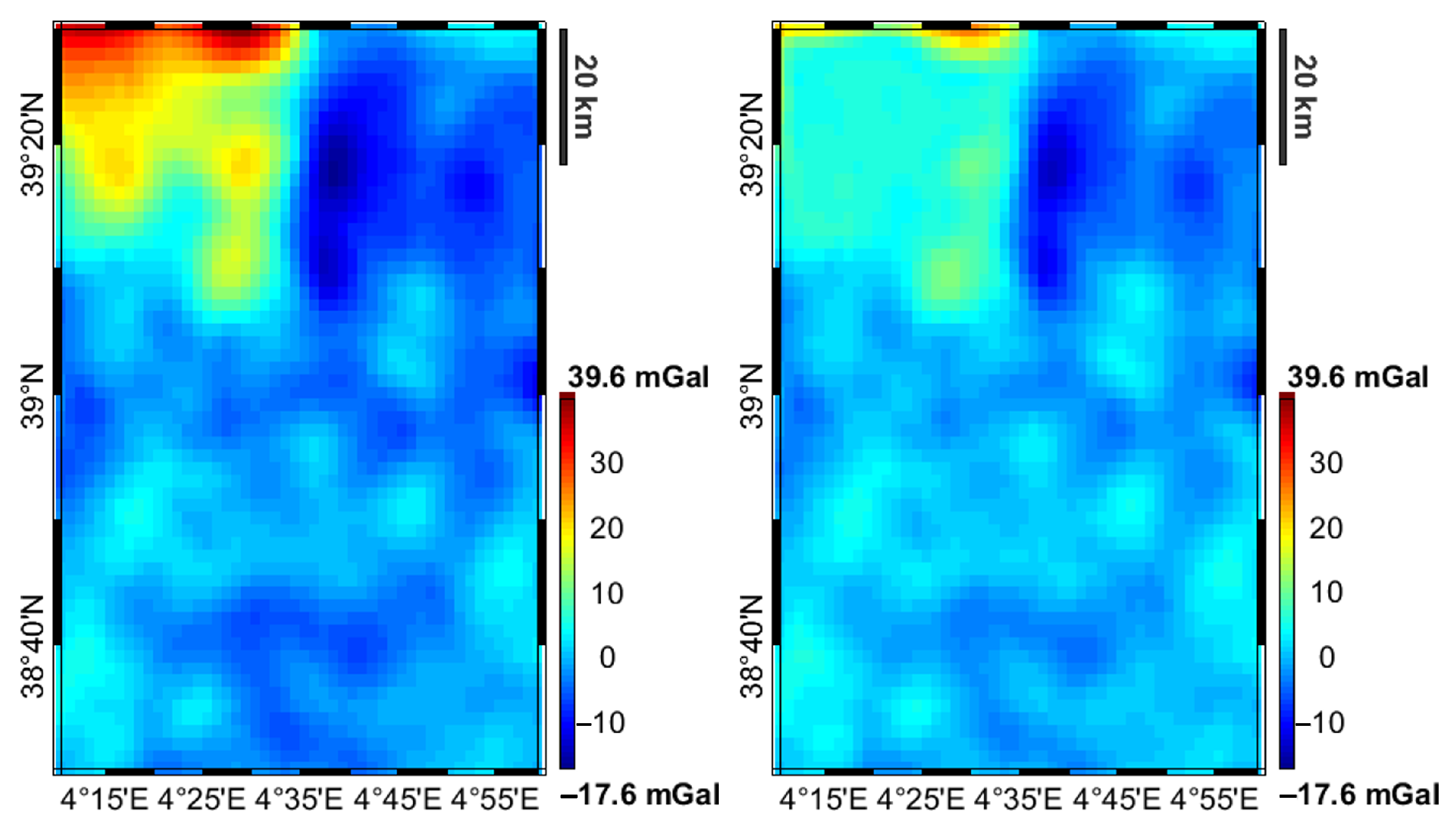
We fixed the maximum depth of the model built to perform the inversion at 3200 m. We then removed from the XGM2019e gravity model, synthesized in terms of gravity anomaly at zero level, the gravitational effect of the density variations around and below the study volume. For this purpose, we exploited the 3D crustal model of the whole Mediterranean region obtained in the European Space Agency XORN project [15]. The resulting gravitational field is shown, together with the original free-air anomalies, in Figure 4.
Within the inversion volume, also the base of Plio-Quaternary and Messinian sediments are present. For these two layers, we used the surfaces estimated in the regional model, supposing an uncertainty of 100 m. As for the density, we used 1030 kg/m 3 for the seawater, and again the crustal model density distribution for the other two layers. Figure 5 shows the residuals in terms of gravity anomaly before and after the inversion.
We note that the residuals, if evaluated in terms of STD, decrease from 8.3 mGal in the a priori model to 4.2 mGal of the a posteriori one. We compare in Figure 6 the true bathymetry with the a priori and a posteriori ones.
The figure shows how the inversion algorithm has improved the a priori bathymetry, without creating artifacts and without modifying the a priori model, where considered reliable. This is confirmed also by the statistics, differences between the a priori and true bathymetry shows an STD of 126.8 m, which decreases to 60.1 m when the differences between the a posteriori and the true model are considered. Before concluding this section, we also report in Figure 7 a 3D representation of the a priori and a posteriori volumes in terms of labels. It is evident that the inversion algorithm not only modifies the seafloor where direct observations are lacking, preserving it unchanged in the other regions, but also slightly alters the shape of the boundary between Plio-Quaternary and Messinian sediments to further improve the gravity fitting.

3.2. Second Test

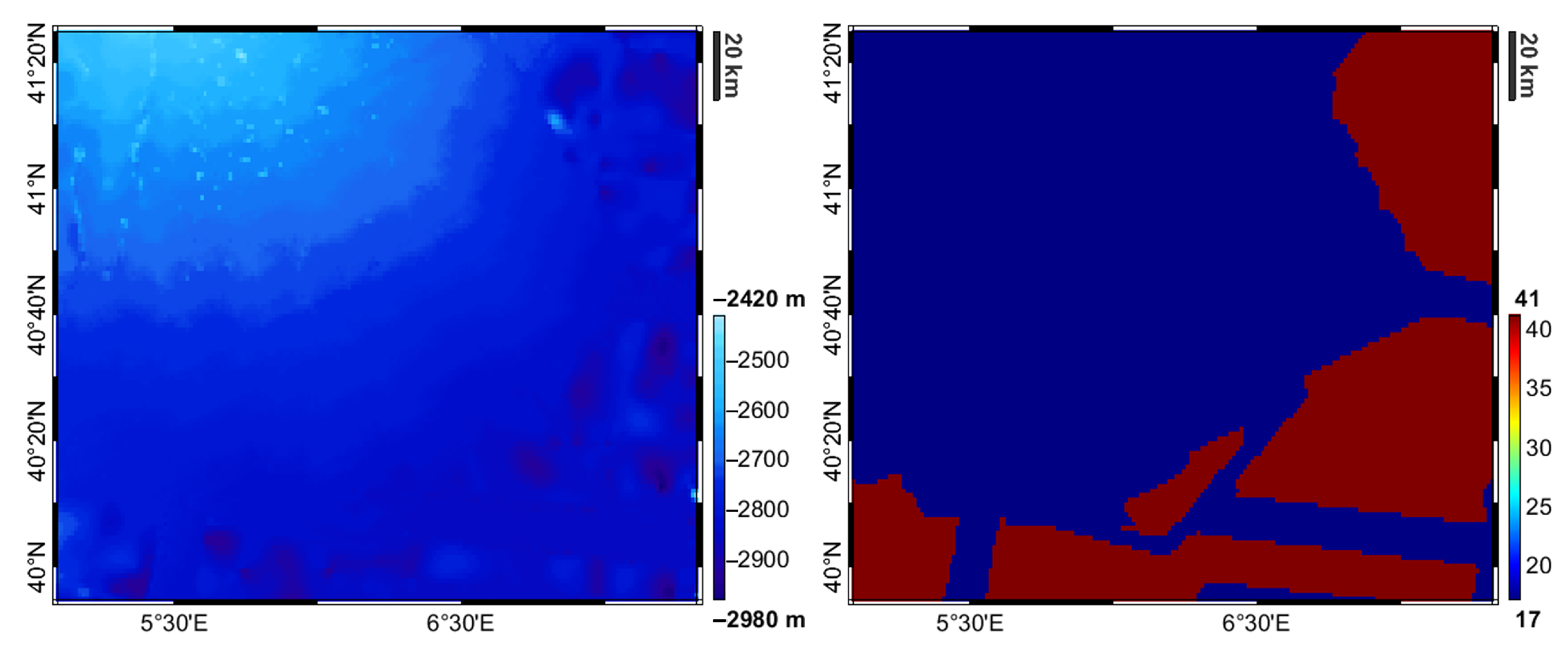
We performed a second test to estimate bathymetry in the area ranging between 5 ° W and 7.5 ° W and 39.9 ° N and 41.4 ° N. The area is characterized by an almost flat bathymetry that deepens from 2340 m to about 3000 m towards the southwest. In the GEBCO model, a large part of the area is obtained by direct observations, whereas the borders are estimated by means of a simple interpolation procedure. The GEBCO bathymetry and the corresponding TID maps are shown in Figure 8.
We noticed from the figure a set of anomalous undulations (probably artifacts) in the region with TID equal to 41. The main objective of the second test was to check whether the proposed algorithm would allow us to obtain a bathymetry model without these artifacts. Similarly to the previous test, we started by interpolating, by means of a kriging procedure, the bathymetry from the points with TID equal to 17 to the whole area. The resulting map, with the corresponding predicted accuracy, is reported in Figure 9.
Following the proposed procedure, we reduced the gravity observations for the deep layers, taken again from the XORN regional model. In this test, we performed the gravity inversion considering as observations gravity anomalies and the second radial derivative of the anomalous potential (for the definition of both these functionals of the gravitational field, we refer to [20]). What we discovered was that the gravity residuals are slightly reduced, from 3.1 mGal and 6.2 E of the a priori model to 2.8 mGal and 5.5 E of the a posteriori one. Note that in any case, in such a flat area, even the residuals for the a priori model are very close to the observation error (3 mGal [3]). In Figure 10 we report the a priori, a posteriori, and GEBCO bathymetry maps.
Similarly to Section 3.1, also for this second test, we report in Figure 11, the a priori and a posteriori 3D model in terms of label.
In addition, in test 2, we see that the inversion has changed not only the bathymetry but also the shape of the boundary between the Plio-Quaternary and the Messinian sediments.

4. Final Remarks and Conclusions

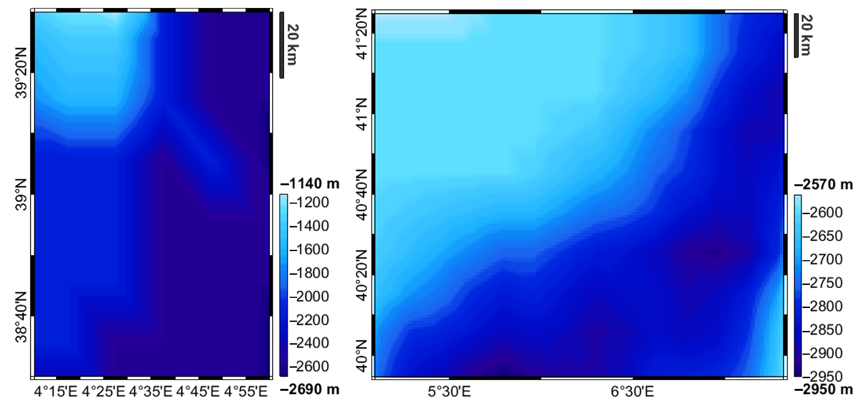
In both the tests performed, the proposed algorithm seemed to give better results than the GEBCO classical procedure. Due to the proposed procedure and the fact that the regional model used to reduce the data was obtained by means of gravity inversion, one can guess that the bathymetry obtained is just a copy of the bathymetry exploited when estimating the regional model. This is not the case for two main reasons: the former is that the spatial resolution of the gravity observations and of the 3D volume used for the regional modeling is coarser than that used for the local inversion, and the latter is that in the local inversion, the new bathymetry is forced by the algorithm to be close (accordingly to the predicted accuracy) to the a priori model. This is confirmed by looking at the bathymetry in the regional model shown in Figure 12.
What we can conclude is that the proposed algorithm allows us to improve (with respect to the classical inversion scheme used, e.g., for the GEBCO global bathymetry) the estimate of bathymetric depths. The main pros are that the procedure is more linear and simpler than the classical algorithm and can be applied in any scenario: it does not suffer from the presence of shelves, continental margins, etc. As for the cons, we have to underline that the procedure requires modeling and stripping the effect of regional density variations from gravity observations. Moreover, the proposed procedure is more demanding in terms of computational time, it required about 8 h for each test on an Intel i3 workstation. However, due to the intrinsic sequentiality of the Gibbs sampler exploited to perform the inversion, only a single processor with just 1 GB of RAM is used. As a consequence of the pros and cons mentioned above, a possibility could be to update the bathymetry with the proposed approach only in the most problematic regions, such as, for instance, in some parts of the Mediterranean Sea area (which are known to be quite complex) that do not have a homogeneous full coverage of direct bathymetric data. In this respect, since the algorithm is based on a planar approximation, and since it requires large computational times to estimate high spatial resolution bathymetry even on relatively small regions, a possible solution is to divide large regions into small patches, similar to those analyzed in the current work, process each patch independently (even in parallel) and then merge the different results. This would allow, for instance, to retrieve an improved bathymetry in the whole Mediterranean Sea region, exploiting the eight cores of our workstation, in less than 15 days. This is even more true since the entire procedure can be automated.

Author Contributions

Conceptualization, D.S. and M.C.; software, D.S. and M.C.; validation, D.S.; data curation, M.C.; writing—original draft preparation, D.S.; writing—review and editing, M.C.; project administration, D.S.; funding acquisition, D.S. and M.C. All authors have read and agreed to the published version of the manuscript.

Funding

This research was funded by the European Space Agency grant number 4000136884/21/I-DT-lr.

Data Availability Statement

XGM2019e model can be downloaded at http://icgem.gfz-potsdam.de/home [21], accessed on 19 September 2022. GEBCO bathymetry data can be downloaded at https://download.gebco.net/ [12], accessed on 19 September 2022.

Conflicts of Interest

The authors declare no conflict of interest. The funders had no role in the design of the study; in the collection, analyses, or interpretation of data; in the writing of the manuscript; or in the decision to publish the results.

References

  1. Tozer, B.; Sandwell, D.T.; Smith, W.H.; Olson, C.; Beale, J.; Wessel, P. Global bathymetry and topography at 15 arc sec: SRTM15+. Earth Space Sci. 2019, 6, 1847–1864. [Google Scholar] [CrossRef]
  2. Smith, W.H.; Sandwell, D.T. Global sea floor topography from satellite altimetry and ship depth soundings. Science 1997, 277, 1956–1962. [Google Scholar] [CrossRef] [Green Version]
  3. Sampietro, D.; Capponi, M.; Thébault, E.; Gailler, L. An empirical method for the optimal setting of the potential fields inverse problem. Geophys. Prospect. 2023, 71, 350–365. [Google Scholar] [CrossRef]
  4. Smith, W. Bathymetric prediction from dense altimetry and sparse shipboard bathymetry. J. Geophys. Res. 1994, 99, 21–803. [Google Scholar] [CrossRef]
  5. Sansó, F.; Sampietro, D. Analysis of the Gravity Field: Direct and Inverse Problems; Birkhäuser: Cham, Switzerland, 2021. [Google Scholar]
  6. Rossi, L. Bayesian Gravity Inversion by Monte Carlo Methods. Ph.D. Thesis, Politecnico di Milano, Milan, Italy, 2017. [Google Scholar]
  7. Sampietro, D.; Capponi, M. Seismic Constrained Gravity Inversion: A Reliable Tool to Improve Geophysical Models Away from Seismic Information. Geosciences 2021, 11, 467. [Google Scholar] [CrossRef]
  8. Sampietro, D.; Capponi, M.; Maurizio, G. 3D Bayesian Inversion of Potential Fields: The Quebec Oka Carbonatite Complex Case Study. Geosciences 2022, 12, 382. [Google Scholar] [CrossRef]
  9. Sampietro, D.; Capponi, M. Practical tips for 3D regional gravity inversion. Geosciences 2019, 9, 351. [Google Scholar] [CrossRef] [Green Version]
  10. Wackernagel, H. Multivariate Geostatistics: An Introduction with Applications; Springer Science & Business Media: New York, NY, USA, 2013. [Google Scholar]
  11. Sampietro, D.; Capponi, M.; Mansi, A.; Gatti, A.; Marchetti, P.; Sansò, F. Space-Wise approach for airborne gravity data modelling. J. Geod. 2017, 91, 535–545. [Google Scholar] [CrossRef] [Green Version]
  12. GEBCO Compilation Group. GEBCO 2020 Grid; British Oceanographic Data Centre, National Oceanography Centre: Liverpool, UK; NERC: Atlanta, GA, USA, 2020. [Google Scholar]
  13. Rexer, M.; Hirt, C.; Pail, R. High-resolution global forward modelling: A degree-5480 global ellipsoidal topographic potential model. In Proceedings of the EGU General Assembly Conference Abstracts, Proceeding of EGU General Assembly 2017, Vienna, Austria, 23–28 April 2017; p. 7725. [Google Scholar]
  14. Zingerle, P.; Pail, R.; Gruber, T.; Oikonomidou, X. The combined global gravity field model XGM2019e. J. Geod. 2020, 94, 66. [Google Scholar] [CrossRef]
  15. Sampietro, D.; Capponi, M.; Thébault, E.; Gailler, L. An enhanced view on the Mediterranean Sea crust from potential fields data. Sci. Rep. 2023, 13, 8298. [Google Scholar] [CrossRef] [PubMed]
  16. Laske, G.; Masters, G.; Ma, Z.; Pasyanos, M. Update on CRUST1.0—A 1-degree global model of Earth’s crust. In Proceedings of the EGU General Assembly 2013, Geophysical Research Abstracts, Vienna, Austria, 7–12 April 2013; Volume 15, p. 2658. [Google Scholar]
  17. Reguzzoni, M.; Sampietro, D. GEMMA: An Earth crustal model based on GOCE satellite data. Int. J. Appl. Earth Obs. Geoinf. 2015, 35, 31–43. [Google Scholar] [CrossRef]
  18. Szwillus, W.; Afonso, J.C.; Ebbing, J.; Mooney, W.D. Global crustal thickness and velocity structure from geostatistical analysis of seismic data. J. Geophys. Res. Solid Earth 2019, 124, 1626–1652. [Google Scholar] [CrossRef]
  19. Fullea, J.; Lebedev, S.; Martinec, Z.; Celli, N. WINTERC-G: Mapping the upper mantle thermochemical heterogeneity from coupled geophysical–petrological inversion of seismic waveforms, heat flow, surface elevation and gravity satellite data. Geophys. J. Int. 2021, 226, 146–191. [Google Scholar] [CrossRef]
  20. Barthelmes, F. Definition of Functionals of the Geopotential and Their Calculation from Spherical Harmonic Models: Theory and Formulas Used by the Calculation Service of the International Centre for Global Earth Models (ICGEM); Deutsches GeoForschungsZentrum GFZ: Potsdam, Germany, 2009; Available online: http://icgem.gfz-potsdam.de (accessed on 19 September 2022).
  21. Ince, E.S.; Barthelmes, F.; Reißland, S.; Elger, K.; Förste, C.; Flechtner, F.; Schuh, H. ICGEM—15 years of successful collection and distribution of global gravitational models, associated services, and future plans. Earth Syst. Sci. Data 2019, 11, 647–674. [Google Scholar] [CrossRef] [Green Version]
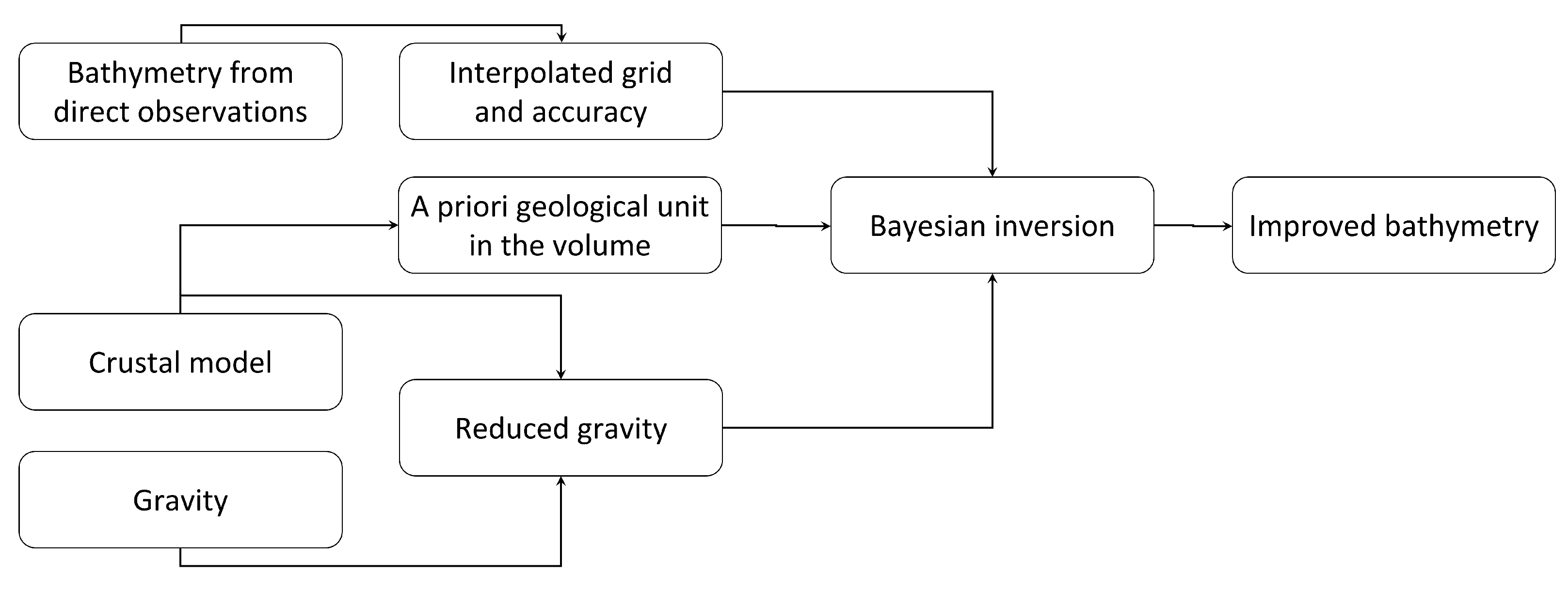
Figure 1. Workflow of the proposed methodology to improve the bathymetry modelling.
Geosciences 13 00223 g001
Figure 2. GEBCO bathymetry depth (left) and TID (right) on the first considered area.
Geosciences 13 00223 g002
Figure 3. A priori bathymetry (left) and predicted accuracy (right).
Geosciences 13 00223 g003
Figure 4. Observed free-air gravity anomaly (left) and gravity anomaly reduced for the regional crustal model (right).
Geosciences 13 00223 g004
Figure 5. Gravity residuals before (left) and after the inversion (right).
Geosciences 13 00223 g005
Figure 6. A posteriori (left), a priori (center) and true (right) bathymetry.
Geosciences 13 00223 g006
Figure 7. A priori (up) and a posteriori (down) volumes for test 1 in term of labels.
Geosciences 13 00223 g007
Figure 8. GEBCO bathymetry (left) and TID map (right).
Geosciences 13 00223 g008
Figure 9. A priori bathymetry (left) and predicted a priori bathymetry accuracy (right).
Geosciences 13 00223 g009
Figure 10. A posteriori (left), a priori (center) and GEBCO (right) bathymetry.
Geosciences 13 00223 g010
Figure 11. A priori (up) and a posteriori (down) volumes for test 2 in term of labels.
Geosciences 13 00223 g011
Figure 12. XORN regional model bathymetry for the first (left) and second (right) test.
Geosciences 13 00223 g012
Table 1. Examples of GEBCO TID.
TIDDefinition
0Land
Direct measurements
10Singlebeam—depth value collected by a single beam echo-sounder
11Multibeam—depth value collected by a multibeam echo-sounder
12Seismic—depth value collected by seismic methods
13Isolated sounding—depth value that is not part of a regular survey or trackline
14ENC sounding—depth value extracted from an Electronic Navigation Chart (ENC)
15Lidar—depth derived from a bathymetric lidar sensor
16Depth measured by optical light sensor
17Combination of direct measurement methods Indirect measurements
Indirect measurements
40Predicted based on satellite-derived gravity data—depth value is an interpolated value guided by satellite-derived gravity data
41Interpolated based on a computer algorithm—depth value is an interpolated value based on a computer algorithm (e.g., Generic Mapping Tools)
Disclaimer/Publisher’s Note: The statements, opinions and data contained in all publications are solely those of the individual author(s) and contributor(s) and not of MDPI and/or the editor(s). MDPI and/or the editor(s) disclaim responsibility for any injury to people or property resulting from any ideas, methods, instructions or products referred to in the content.