Abstract
Constraining the timing and rate of Laurentide Ice Sheet (LIS) retreat through the northeastern United States is important for understanding the co-evolution of complex climatic and glaciologic events that characterized the end of the Pleistocene epoch. However, no in situ cosmogenic 10Be exposure age estimates for LIS retreat exist through large parts of Connecticut or Massachusetts. Due to the large disagreement between radiocarbon and 10Be ages constraining LIS retreat at the maximum southern margin and the paucity of data in central New England, the timing of LIS retreat through this region is uncertain. Here, we date LIS retreat through south-central New England using 14 new in situ cosmogenic 10Be exposure ages measured in samples collected from bedrock and boulders. Our results suggest ice retreated entirely from Connecticut by 18.3 ± 0.3 ka (n = 3). In Massachusetts, exposure ages from similar latitudes suggest ice may have occupied the Hudson River Valley up to 2 kyr longer (15.2 ± 0.3 ka, average, n = 2) than the Connecticut River Valley (17.4 ± 1.0 ka, average, n = 5). We use these new ages to provide insight about LIS retreat timing during the early deglacial period and to explore the mismatch between radiocarbon and cosmogenic deglacial age chronologies in this region.
1. Introduction
Accurately constraining Laurentide Ice Sheet (LIS) retreat is important for understanding the co-evolution of the inter-related climatic, oceanographic, and glacial events during the late glacial period [1], the impact of LIS deglaciation on ocean water volume and thus sea level [2,3], and local impacts on landscape evolution [4]. The southeastern LIS covered the New England region of the northeastern United States during Marine Isotope Stage 2 ([5]; Figure 1), expanding to its southernmost extent by at least 27 to 24 ka (thousand years ago) [6,7,8,9,10]. Following the Last Glacial Maximum (LGM), the LIS margin retreated northward through New England [5,11]. The exact timing of the LIS retreat initiation in New England is debated but is often interpreted to have started by at least 20 ka [1,5,12], despite persistent stadial conditions in the Northern Hemisphere until approximately 17 ka [13]. Complicating the uncertainty is a 10 kyr difference between the organic 14C ages and in situ 10Be exposure ages estimating LIS retreat initiation near its terminal moraine [10,14,15].
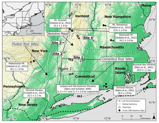
Figure 1.
Map showing study location and regional topography in northeastern North America. Field sites from this study are marked (open white circles) as well as previous work in New England using in situ 10Be exposure dating [1,7,14,16] (solid black circles; recalculated using LSDn scaling and global production rate where necessary). Thick dashed line represents the LIS terminal moraine as mapped by Dyke et al. [11]; thin dashed lines represent retreat isochrons during the last deglacial period, with estimated ages (ka) shown in bold numbers, from Dalton et al. [5]. Additional locations described in the text are labeled for regional context.
Despite the relatively large number of glacier chronology studies in New England, a lack of 10Be exposure dating through most of Connecticut and Massachusetts makes LIS retreat timing (and corresponding timing to regional climate) less certain [10,16]. Glacial retreat in central New England is dated only by organic 14C in central Massachusetts [17,18,19] and the New North American Varve Chronology (NAVC) in the Connecticut River Valley (Figure 2; [12]). There are no 10Be age constraints between the Ledyard Moraine (abandoned 21.4 ± 0.7 ka; Figure 1) and the Old Saybrook Moraine (abandoned 21.3 ± 0.9 ka; Figure 1) in southern Connecticut [1] and Mt. Greylock (15.2 ± 1.4 ka; Figure 1) in northern Massachusetts [16]. This leaves a spatial gap in the 10Be chronology of approximately 125 km and more than 6 kyr, coinciding with the timing of LIS retreat during a changing late glacial New England climate [20,21]. Furthermore, the presence of two different ice lobes (one in the Hudson and the other in Connecticut River Valley, separated by the Berkshire Massif in Massachusetts) likely leads to more complexity in LIS marginal positions than is represented by larger-scale reconstructions (e.g., [5,11]; Figure 1).
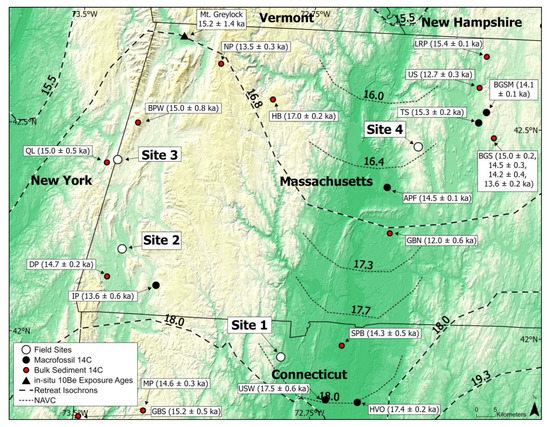
Figure 2.
Map showing local topography around field sites (open white circles) and current deglacial constraints (in ka) based on Dalton et al. [5] (large black and white dashed lines) and Ridge et al. [12] (small black dashed lines). We identify all previously published, minimum-limiting deglacial organic 14C ages (see Table 1, solid black circles and red circles with black outline), with abbreviated names corresponding to the table entries and 10Be exposure ages (solid black triangle; Halsted et al. [16]) from the region.
To understand better the history of the LIS retreat through northern Connecticut and Massachusetts, we determined the timing of deglaciation using 14 new in situ 10Be exposure ages from 11 boulders and 3 bedrock samples. Our data, which fills an existing spatial gap, allow us to make inferences about the position of the LIS margins in central New England between 20 ka and 15 ka, coinciding with the onset of major deglaciation in the Northern Hemisphere [3,22].

Table 1.
Compilation of previously published organic 14C ages used to provide minimum limiting ages of deglaciation for the LIS in the study area.
Table 1.
Compilation of previously published organic 14C ages used to provide minimum limiting ages of deglaciation for the LIS in the study area.
| Location | Map Code | Latitude (°N) | Longitude (°W) | Elevation (m) | Material Type | 14C Age and Uncertainty (14C yr BP) * | Calibrated Age and Uncertainty (yr BP) ** | Reference and Sample ID |
|---|---|---|---|---|---|---|---|---|
| Amherst, MA | APF | 42.360 | 72.510 | 43 | Terrestrial plant fragments | 12,370 ± 120 | 14,500 ± 120 | Rittenour [19], Beta-124780 |
| Black Gum Swamp, MA | BGS | 42.480 | 72.167 | 357 | Bulk Sediment | 12,400 ± 80 | 14,520 ± 270 | Anderson et al. [23], AA-40809 |
| Black Gum Swamp, MA | BGS | 42.480 | 72.167 | 357 | Bulk Sediment | 12,610 ± 80 | 15,000 ± 150 | Anderson et al. [23], AA-40812 |
| Black Gum Swamp, MA | BGS | 42.480 | 72.167 | 357 | Bulk Sediment | 11,690 ± 140 | 13,560 ± 160 | Foster and Zebryk [24], Beta-31366 |
| Black Gum Swamp, MA | BGS | 42.480 | 72.167 | 357 | Bulk Sediment | 12,240 ± 110 | 14,240 ± 380 | Anderson et al. [23], Beta-42117 |
| Black Gum Swamp, MA | BGSM | 42.542 | 72.192 | 358 | Picea fragments | 12,190 ± 60 | 14,100 ± 70 | Lindbladh et al. [18], Beta-192020 |
| Berry Pond, MA | BPW | 42.506 | 73.319 | 631 | Bulk Sediment | 12,680 ± 480 | 15,040 ± 750 | Whitehead [25], OWU-481 |
| Davis Pond, MA | DP | 42.136 | 73.408 | 213 | Bulk Sediment | 12,500 ± 50 | 14,700 ± 210 | Newby et al. [26,27], OS-55125 |
| Granby Bog, MA | GBN | 42.250 | 72.500 | 110 | Bulk Sediment | 10,300 + 370 | 12,020 ± 610 | Valastro et al. [26], TX-2946 |
| Gross Bog, CT | GBS | 41.800 | 73.491 | 330 | Bulk Sediment | 12,750 ± 230 | 15,160 ± 500 | Newman et al. [28], RL-245 |
| Hawley Bog, MA | HB | 42.567 | 72.883 | 549 | Bulk Sediment | 14,000 ± 130 | 17,020 ± 220 | Bender et al. [29], WIS-1122 |
| Hitchcock Varve Outcrop, CT | HVO | 41.845 | 72.598 | 0 | Terrestrial plant leaves, mostly Dryas integrifolia | 14,300 ± 60 | 17,390 ± 150 | Ridge et al. [12], OS-77140 |
| Ivory Pond, MA | IP | 42.117 | 73.250 | 0 | Picea glauca cones | 11,630 ± 470 | 13,640 ± 570 | Moeller [17], GX-9259 |
| Little Royalston Pond, MA | LRP | 42.675 | 72.192 | 362 | Bulk Sediment | 12,910 ± 80 | 15,440 ± 130 | Oswald et al. [30], AA-58099 |
| Mohawk Pond, CT | MP | 41.817 | 73.283 | 360 | Bulk Sediment | 12,460 ± 110 | 14,630 ± 300 | Steventon and Kutzbach [31], WIS-1405 |
| North Pond, MA | NP | 42.650 | 73.053 | 586 | Bulk Sediment | 11,600 ± 280 | 13,500 ± 290 | Huvane and Whitehead [32], GX-4490 |
| Queechy Lake, NY | QL | 42.408 | 73.417 | 311 | Bulk Sediment | 12,680 ± 200 | 15,040 ± 450 | Stuiver [33], Y-2247 |
| Suffield Peat Bog, CT | SPB | 41.980 | 72.650 | 47 | Bulk Sediment | 12,200 ± 350 | 14,340 ± 540 | Rubin and Alexander [34], W-828 |
| Tom Swamp, MA | TS | 42.517 | 72.217 | 232 | Vascular plant macrofossils | 12,830 ± 120 | 15,330 ± 180 | Miller [35], WIS-1210 |
| Unnamed Swamp, MA | US | 42.601 | 72.215 | 212 | Bulk Sediment | 10,800 ± 250 | 12,740 ± 300 | Rubin and Alexander [36], W-361 |
| Unnamed Pond, CT | USW | 41.850 | 72.700 | 0 | Salix wood fragments | 14,330 ± 430 | 174,70 ± 560 | Stone and Ashley [37], Beta-35211 |
* 14C ages (uncalibrated) as reported in source publications. BP = years before present (1950 AD). ** Calibrated years before present (calendar years before 1950 AD) were calculated using the MatCal software from Lougheed and Obrochta, [38] and the IntCal20 calibration curve from Reimer et al. [39]. Uncertainties reported here are one half of the 68.2% probability distribution range of calibrated ages.
2. Background
2.1. Geographic Setting: Connecticut River and Hudson River Valleys
The study area encompasses sites in north-central Connecticut and west-central Massachusetts (Figure 2) within the Connecticut River and Hudson River Valleys that hosted LIS lobes and, later, large glacial lakes [12,40]. These valleys are separated by the Berkshire Massif [41], which is ~600 m higher than the Hudson River Valley and ~550 m higher than the Connecticut River Valley, possibly attributable to erosion-resistant metamorphic and igneous bedrock underlying the upland [42]. During deglaciation, the Hudson and Connecticut River Valleys constrained and channeled ice flow parallel to regional topography, resulting in south-flowing ice lobes from the LIS that persisted longer in the lowlands than in the highlands [5,11,12,16,43]. Upland areas, where bedrock is not exposed at the surface, are mantled by till [43], and often contain large boulders suitable for cosmogenic nuclide dating. In lowland areas, drainage basins trapped glacio-lacustrine sediment in proglacial lakes, allowing for the deposition of rhythmic glacial sediment, interpreted as varves [40,44,45].
2.2. In Situ Cosmogenic Nuclide Exposure Dating
The accumulation of cosmogenic nuclides in rocks exposed to cosmic rays at the Earth’s surface is used to estimate exposure duration and therefore to determine the timing of past geomorphic events [46,47]. Spallation reactions occurring in minerals (for example, quartz) bombarded by cosmic rays result in the production of cosmogenic nuclides at and near the Earth’s surface [48,49]. During ice occupation in formerly glaciated regions, cosmogenic nuclides do not accumulate due to the shielding of rock surfaces by overriding ice [50]. When the ice retreats and surfaces are exposed, cosmogenic nuclides accumulate at predictable rates [46]. Measuring the concentration of specific cosmogenic nuclides (most commonly 10Be) provides insight about the duration of exposure following ice retreat [1,14,49,51].
The use of cosmogenic nuclide dating to constrain the timing of glacial retreat depends on the assumptions of the material being dated. One assumption is subglacial erosion occurred deep enough to remove in situ 10Be produced during prior periods of exposure. Where warm-based ice occupies the landscape for thousands of years, meters of erosion occur, reducing the 10Be concentration in outcrops to low levels [50]. However, if ice is cold-based and non-erosive, and/or has a short period of occupation, erosion depth is limited and nuclides from previous exposure periods can remain in rocks [52,53]. If 10Be from prior periods of exposure is not removed by erosion, calculated exposure ages will overestimate the true timing of deglaciation [51,54]. If boulders are disturbed (e.g., rolled) or shielded following exposure, and then subsequently exhumed, exposure ages will underestimate the timing of local deglaciation [55].
2.3. Previous Work: LIS Retreat Timing in New England
Early work to constrain ice retreat through New England relied on stratigraphic relationships and sedimentological observations [44,45,56,57,58,59]. With the advent of numerical dating methods, current constraints on deglaciation in most of Massachusetts and Connecticut now rely on glacial varve chronologies [12,44,45] and organic 14C ages (from bulk sediment or macrofossil samples) from the bottom of lake or bog sediment cores [5,11,15]. Organic 14C ages indicate the timing of post-glacial re-vegetation and are often interpreted as minimum limits on the timing of local deglaciation [60]. 14C ages from both bulk sediment and macrofossil samples are used in New England deglacial chronologies, but age discrepancies between these methods have previously been noted [10,15]. Older bulk sediment ages are often attributed to incorporation in samples of carbon-bearing materials unrelated to deglaciation [61], and so younger 14C ages from macrofossil samples are typically viewed as more accurately corresponding to the timing of post-glacial re-vegetation [15]. Both radiocarbon and varve-based chronologies suggest that ice retreated fully from Connecticut by 17.5–17.7 ka and from Massachusetts by 15.5 ka [5,12]. The North American Varve Chronology (NAVC) utilizes organic 14C ages to anchor it to calendar years and Dalton et al.’s [5] chronology is based on the NAVC, adjusting the margins from Dyke’s [11] isochrons and then extending them east and west of the Connecticut River Valley. More recent studies utilize in situ 10Be exposure ages from erratic boulders, moraine boulders, or glacially scoured bedrock to estimate the timing of ice retreat; however, there are no published cosmogenic nuclide data in central New England [1,14,51,62,63,64].
2.4. Paleoclimate during LIS Retreat through New England
The global climate system changed significantly after the LGM. Summer insolation began increasing ~24 ka at high northern latitudes [13,65], increasing the duration and intensity of radiative forcing over the LIS [66]. Northward oceanic heat transport via the Gulf Stream was strong during the LGM but weakened significantly from 19 to 15 ka [67], reducing oceanic heat supply off the New England coast. Atmospheric CO2 concentrations began increasing globally approximately 17 ka and were a major driver of Northern Hemisphere warming during deglaciation [68]. However, prior to 17 ka, global mean surface temperatures remained cold, particularly in regions surrounding the North Atlantic [13,66].
3. Study Sites
Our work focuses on four study sites within New England (Figure 1). We selected one site in Connecticut within the Connecticut River Valley Basin (Site 1) and three sites in Massachusetts: two in or near the Hudson River Valley (Sites 2 and 3) and one in the Connecticut River Valley (Site 4; Figure 2). All sites are above glaciolacustrine limits and are spatially separate, forming two N-S trending profiles allowing us to assess the LIS as it retreated northward at the end of the LGM. Additionally, sampling from two separate river valleys allows us to assess the dynamics of sub-lobes of the LIS.
3.1. Connecticut River Valley, Northern Connecticut (Site 1)
We collected samples from two schist bedrock outcrops and two boulders (one schist and one granite) near Broad Hill in West Granby, Connecticut (41°57.37′ N, 72°50.64′ W). Sampling occurred near a 20 m cliff face with scree scattered near the base. We sampled boulders more than 500 m away from the cliff face to minimize the possibility that boulders were emplaced by rock fall off the cliff and instead are part of the surficial till. The landscape away from the cliff is hummocky and has abundant large rounded to subrounded boulders present at the surface (Figure 3). Intermittent bedrock outcrops of the Goshen formation (Devonian schist; [69]) are visible at the surface and contain abundant quartz veins that protrude 2–3 cm in positive relief.
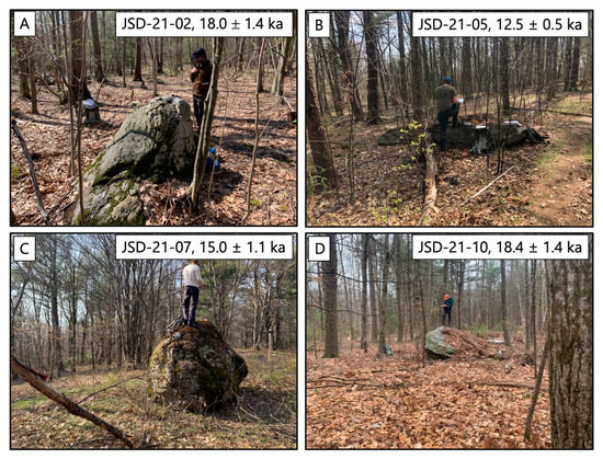
Figure 3.
Representative samples from each study site showing the relatively flat deciduous forest landscape where we collected samples. (A) Connecticut River Valley in Northern Connecticut (Site 1; n = 4), (B) Housatonic Valley in Western Massachusetts (Site 2; n = 1), (C) Hudson River Valley drainage divide in Western Massachusetts (Site 3; n = 4), (D) Connecticut River Valley in Central Massachusetts (Site 4; n = 5). Labels show sample ID and exposure age ± external uncertainty.
3.2. Housatonic Valley, Western Massachusetts (Site 2)
We collected one sample from the quartz vein on top of a schist boulder near Lake Mansfield in Great Barrington, Massachusetts (42°12.206′ N, 73°22.069′ W) located in the Housatonic Valley of western Massachusetts (the watershed bordering the Hudson River Valley in the east). This site was selected due to the presence of the Great Barrington Boulder Train identified in 1910 by Frank Taylor [70]. The local topography is low relief (less than 50 m elevation change) with some boulders (5 m in diameter) scattered at the surface (Figure 3). The site is near the Housatonic River, but well above its floodplain, and boulders occur on a local topographic high, suggesting that no post-glacial movement following deposition occurred.
3.3. Hudson River Valley Drainage Divide, Western Massachusetts (Site 3)
We sampled one phyllite bedrock outcrop and three boulders (one phyllite and two quartz veins on schist) near Perry’s Peak in Richmond, Massachusetts (42°24.823′ N, 73°22.771′ W). Located on a ridge of the Nassau Formation [71], the site is ~400–500 m above the Hudson River Valley to the west on the drainage divide with the Housatonic Valley ~200–300 m below to the east. Few boulders are present, despite the literature suggesting that this region was rich in boulders from the Richmond Boulder Train [70]. Boulders did not appear to represent the Nassau formation, so were likely erratic. However, this land was farmed extensively in the 18th and 19th centuries, as indicated by the presence of stone walls. At that time, farmers may have moved the boulders. Few bedrock outcrops were present, mostly at higher elevations.
3.4. Connecticut River Valley, Central Massachusetts (Site 4)
We sampled five boulders near Shutesbury, Massachusetts (42°27.472′ N, 72°24.694′ W). The study site is on the upland between the Ashuelot and Chicopee River watersheds, both of which drain into the Connecticut River Valley. This location was above the paleo-shoreline of Glacial Lake Hitchcock. Large boulders are scattered across the area, some in very close proximity to each other; all are coarse-grained gneiss with large quartz veins (Figure 3). The terrain is hummocky, possibly due to kame and kettle terrain formed during ice retreat.
4. Methods
4.1. Field Sampling
We sampled boulders (n = 11) and bedrock (n = 3) from the four sites in April 2021 (Table 2). Sub-rounded boulders, assumed to be glacially entrained, were selected if they showed no indication of post-glacial movement, shielding, or sub-aerial erosion. We selected bedrock in locations near boulders and only where there was no evidence of post-glacial shielding by soil or sediment. We removed the top few centimeters of rock with a hammer and chisel. We recorded site parameters for 10Be production rate estimation, including latitude, longitude, elevation, rock surface strike and dip at the sampled location, and the azimuth and elevation of local topography for shielding calculations using the online topographic shielding calculator described in Balco et al. [72].
Table 2.
Sample location and field data for 14 boulder and bedrock samples.
4.2. Sample Preparation and Measurement
We measured the average sample thickness for each sample, and then isolated quartz at the University of Vermont according to methods described in Kohl and Nishiizumi, [73]. We verified quartz purity using a Perkin Elmer, Avio 200 Inductively Coupled Plasma Optical Emission Spectrometer. We isolated and purified beryllium at the National Science Foundation/University of Vermont Community Cosmogenic Facility with the methods described in Corbett et al. [74]. We prepared samples in two separate batches, each including one blank and one liquid reference material [75]. We digested between 17.5 and 21.1 g of quartz and added 250 µg 9Be to each using an in-house diluted carrier, termed UVM-SPEX, created from the dilution of SPEX 10,000 ppm Be standard, with a resulting concentration of 304 µg mL−1 (Table 3).
Table 3.
Sample preparation and laboratory information for 10Be/9Be analysis.
Accelerator Mass Spectrometer (AMS) measurements of 10Be/9Be were performed at Purdue Rare Isotope Measurement (PRIME) Laboratory. Samples were normalized to the primary standard of 07KNSTD3110 with an assumed 10Be/9Be ratio of 2.850 × 10⁻¹² [76]. Measured sample ratios ranged from 5.19 × 10⁻¹⁴ to 12.2 × 10⁻¹⁴. We corrected for backgrounds by subtracting the blank ratio (3.40 ± 0.68 × 10⁻¹⁵) from the sample ratios and propagating uncertainties in quadrature.
4.3. Age Calculation
Exposure age estimates were calculated using Version 3 of the online exposure age calculator described in Balco et al. [72], calculated with the global production rate from Borchers et al. [77], using the LSDn scaling scheme from Lifton et al. [78], and assuming a quartz density of 2.65 g cm−3. We selected the global production rate because we are comparing ages to organic 14C dates and the North American Varve Chronology, both of which were used to calibrate the Northeastern North America production rate [79]. Exposure ages assume no nuclide inheritance from previous exposure and that no shielding or erosion occurred since deglaciation. We assessed for outliers using the iceTEA “Remove Outliers” tool from Jones et al. [80].
5. Results
Cosmogenic exposure ages range from 12.5 ± 0.7 ka to 22.4 ± 1.7 ka (Table 4; Figure 4 and Figure 5; internal uncertainties). Given independent constraints on the LIS margin reaching northern New England by at least 14 ka, (e.g., [12,16,51,62,81,82,83]), we exclude three implausibly young values (JSD-21-07 from Site 2, and JSD-21-08 and JSD-21-09 from Site 3; Table 4; Figure 5). These boulders may have been disturbed following glacial retreat by widespread anthropogenic landscape change that occurred in the 17th–20th centuries in New England and resulted in the movement and removal of boulders to clear fields for agriculture [84]. In addition, these boulders may have experienced partial shielding by soil thus causing measured ages to record processes other than simple exposure.
Table 4.
Calculated exposure ages based on in situ 10Be concentrations.
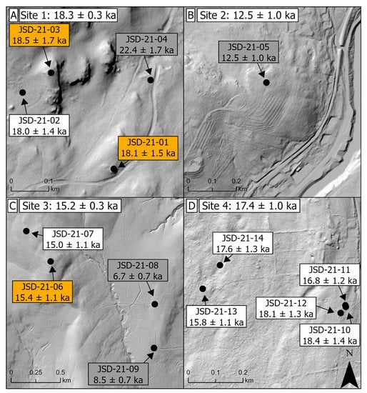
Figure 4.
Map of each of four field sites showing sample locations overlain on 1 m LiDAR hillshade. Calculated exposure age ± external uncertainty for each sample and average of accepted samples ± 1 SD for each site. Samples with orange highlight are bedrock, all other samples are boulders. Samples that we consider outliers are indicated by a grey background. (A) Site 1—Northern Connecticut in the Connecticut River Valley, (B) Site 2—Western Massachusetts in the Housatonic River Valley, (C) Site 3—Western Massachusetts on the Hudson River Valley drainage divide, (D) Site 4—Central Massachusetts in the Connecticut River Valley.
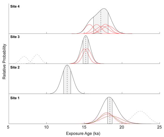
Figure 5.
Kernel density functions of exposure ages for each site in this study (black). Probability density functions for individual 10Be ages are plotted in red. Ages identified as outliers are plotted as gray dashed lines.
The average exposure age for Site 1 in the Connecticut River Valley near the Connecticut and Massachusetts border is 18.3 ± 0.3 ka (n = 3; mean ± 1 SD; Figure 5). Bedrock (18.3 ± 0.3 ka, n = 2; mean ± 1 SD) and boulder (20.2 ± 3.1 ka, n = 2) samples agree within uncertainties. According to a two-tailed generalized extreme Studentized deviate test [80], sample JSD-21-04 was identified as an outlier at Site 1. This may be explained by inheritance from previous exposure; however, due to the small sample size, it is difficult to confidently discard this sample as an outlier; if it is included, the average exposure age for Site 1 becomes 19.3 ± 2.1 ka (n = 4; mean ± 1 SD). For Site 2 in western Massachusetts, there is a single 12.5 ± 0.7 ka (internal uncertainty) sample (Table 4; Figure 4). At Site 3 in Western Massachusetts north of Site 2, the average age of samples is 15.2 ± 0.3 ka (n = 2). Site 4 in the Connecticut River Valley has an average exposure age of 17.4 ± 1.0 ka (n = 5).
The distributions of ages in the Connecticut and Hudson River Valleys appear to differ from one another. Samples from northern Connecticut (Site 1) suggest exposure by 18.3 ± 0.3 ka. Samples from Central Massachusetts, 60 km north (Site 4), suggest exposure by at least 17.4 ± 1.0 ka (Figure 2). Samples from Site 3 in the Hudson River Valley suggest exposure occurred 15.2 ± 0.3 ka, which is approximately 2 kyr later than at Site 4 at a similar latitude in the Connecticut River Valley (Figure 2 and Figure 5).
6. Discussion
6.1. Regional Significance of Exposure Ages
Exposure ages from study sites in the Connecticut River Valley decrease from south to north (Figure 5), but deglaciation in the central Connecticut River Valley (17.4 ± 1.0 ka, n = 5, Site 1) may have occurred earlier than in the Hudson River Valley at a similar latitude (15.2 ± 0.3, n = 2, Site 3). The small number of samples at each site limits our ability to reliably constrain retreat timing differences between the two lobes. Samples in the Connecticut River Valley support deglaciation to the border of Connecticut and Massachusetts by 18.3 ± 0.3 ka (Site 1, n = 3), with the LIS margin reaching central Massachusetts by 17.4 ± 1.0 ka (Site 1, n = 5). Given the uncertainty on ages for these two sites, our ages suggest rapid ice sheet retreat through this area. Other reconstructions suggest that ice retreated at approximately the same time through these valleys [5,12].
The sample sites we explore here are bracketed in southern Connecticut by the cosmogenic exposure ages from the Ledyard (21.4 ± 0.7 ka) and Old Saybrook (21.3 ± 0.9 ka) moraines [1] and Mt. Greylock in northern Massachusetts (15.2 ± 1.4 ka) [16]; hence, our data fill in the previously existing gap in the 10Be exposure age chronology in New England (Figure 6). Considered together, the cosmogenic data suggest continuous and likely rapid ice sheet retreat through Connecticut and Massachusetts between 20 and 15 ka, a time when persistently cold stadial conditions existed in the region.
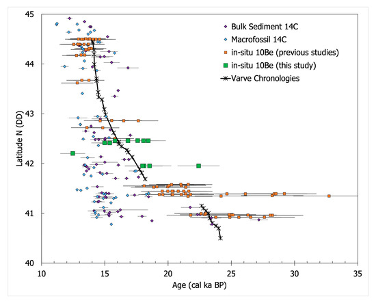
Figure 6.
Plot of age versus latitude for all samples corresponding to LIS deglaciation in New England. New ages for this study are in green and fill a conspicuous hole in the previously published 10Be chronology (ages for JSD-21-08 and -09 are not shown). 10Be exposure ages agree better with the varve chronology than organic radiocarbon ages. The results of all three chronometers converge to the north. All 14C values are recalibrated using the same method as described in Table 1.
6.2. Comparison to Other Regional LIS Retreat Chronologies
Our findings are consistent with the NAVC; both records suggest similar timing for deglaciation and thus the rate of LIS retreat in the Connecticut River Valley. At the southernmost site (1), the ice retreated by 18.3 ± 0.3 ka and reached the northernmost site (~60 km distance, Site 4) at approximately 17.4 ± 1.0 ka. This chronology is similar to, but slightly older than, that suggested by the NAVC, which places ice retreat from northern Connecticut by 18.0 ka and central Massachusetts by 16.4 ka, within the uncertainty of our calculated values. Ice retreat rates estimated from exposure ages are similar to those estimated by the NAVC estimates; we calculate a most-likely retreat rate of 67 m y−1 north (range: 27–>100 m y−1) through the Connecticut River Valley; the range estimated by Ridge et al. [12] through this same region is 30–40 m y−1. Our choice of 10Be production rate calibration data set (Section 4.3) could explain why the most-likely exposure ages are slightly older than the ice retreat dates suggested by the NAVC, as could 10Be inherited from prior periods of exposure. The global calibration data set that we use here [77] implies slightly lower 10Be production rates (~4%), and thus older calculated exposure ages (~0.7 kyr), for central New England compared to a regional calibration data set based on the NAVC ([79]; with LSDn scaling).
Although these new cosmogenic ages align reasonably with NAVC-based retreat dates, they do not always agree well with existing core bottom radiocarbon ages (Figure 2 and Figure 6). Near Site 1 in the Connecticut River Valley near the Connecticut-Massachusetts border, the oldest calibrated radiocarbon ages from macrofossils are 17.5 ± 0.6 ka (USW) and 17.4 ± 0.2 ka (HVO), nearly 1 ka younger than exposure ages slightly farther north (Table 1; Figure 2). At Site 4 in central Massachusetts, the average exposure age is 17.4 ± 1.0 ka, but nearby radiocarbon samples are 14.5 ± 0.1 ka (APF; macrofossil; Figure 2), 15.3 ± 0.2 ka (TS; macrofossil; Figure 2), and 15.0 ± 0.2 ka (BGS; bulk sediment; Figure 2), or 2–3 ka younger. Despite the differences in deglacial ages between chronologies in the Connecticut River Valley, radiocarbon ages agree better at Site 3 in Western Massachusetts. Two radiocarbon ages from bulk sediment nearby are 15.0 ± 0.8 ka (BPW; Table 1; Figure 2) and 15.0 ± 0.5 (QL; Table 1; Figure 2) agreeing with the 15.2 ± 1.6 ka cosmogenic estimate of ice retreat there. Delayed revegetation of the landscape following the initial LIS retreat may account for the larger differences between radiocarbon dates and new exposure ages in the older Connecticut River Valley site (e.g., [10]).
6.3. Possible Paleoclimate Forcings on LIS retreat
The timing of LIS retreat through Connecticut and Massachusetts between 18.3 and 15.2 ka is coincident with a cold stadial period across the Northern Hemisphere [13]. Existing paleoclimate reconstructions suggest that prior to 17 ka, rising summer insolation was the primary driver of deglaciation [13,66]. Some suggest that LIS retreat during a cold period is unlikely and thus conclude, based on radiocarbon ages, that LIS retreat did not begin until approximately 16 ka [15]. However, the change in solar insolation starting at 24 ka [65] has been linked to LIS recession elsewhere along the southern margin [66]. Following the initial retreat of the LIS, the Gulf Stream slowed significantly beginning at approximately 19 ka, bringing less warmth from the equatorial regions to the North Atlantic. Despite this, we measure exposure ages from northern Connecticut at approximately 18.3 ka, prior to the onset of major global deglaciation at 17 ka due to rising CO2. Additionally, we find exposure ages from central Massachusetts, 60 km north, 2 kyr later, suggesting that during this period the LIS in New England was actively retreating. Retreat during this time is supported by the NAVC. Together, these observations suggest that rising summer insolation, identified elsewhere as being responsible for LIS retreat [66], may be a cause for margin retreat in central New England as well, given that we date retreat prior to the re-strengthening of the Gulf Stream and rising CO2 levels.
7. Conclusions
Constraining the timing of deglaciation of the LIS in central New England is important for understanding the co-evolution of regional climate with deglaciation at the end of the Last Glacial Maximum. Fourteen new in situ 10Be exposure ages from Northern Connecticut and Massachusetts fill a conspicuous gap in cosmogenic dates of LIS retreat and allow a better understanding of the LIS and climate co-evolution at the end of the LGM. We determined that ice in the Connecticut River Valley retreated from Connecticut by approximately 18.3 ka and retreated ~60 km north through central Massachusetts by 17.4 ka. In western Massachusetts, ice from the Hudson Valley lobe reached a similar latitude by 15.2 ka. These data suggest that the LIS margin in central New England continued retreating during a stadial period when the Gulf Stream was weak, and the Northern Hemisphere was cold.
Author Contributions
Conceptualization, J.S.D., C.T.H. and P.R.B.; methodology, L.B.C. and P.R.B.; formal analysis, J.S.D. and C.T.H.; investigation, J.S.D., C.T.H., L.B.C. and M.W.C.; resources, L.B.C., P.R.B. and M.W.C.; data curation, C.T.H.; writing—original draft preparation, J.S.D.; writing—review and editing, C.T.H., L.B.C., P.R.B. and M.W.C.; visualization, J.S.D. and C.T.H.; supervision, C.T.H., L.B.C. and P.R.B.; project administration, P.R.B.; funding acquisition, J.S.D. and P.R.B. All authors have read and agreed to the published version of the manuscript.
Funding
This research was funded by the University of Vermont (UVM) Geology Department, Hawley Mudge grant; UVM College of Arts and Sciences, APLE Award; the Geological Society of America Northeastern Section, Stephen G. Pollock Undergraduate Student Research Grant; UVM Summer Undergraduate Research Fellowship, Sustainability Summer Fellowship; and by funding provided to P.R.B. by the National Science Foundation under NSF-EAR-1735676 and NSF-EAR-1602280.
Data Availability Statement
Data associated with this project will be made available on the ICE-D: Laurentide database upon publication of this work. ICE-D can be accessed at ice-d.org.
Acknowledgments
We thank Al Werner for his assistance finding suitable boulders to sample in Western Massachusetts.
Conflicts of Interest
The authors declare no conflict of interest. The funders had no role in the design of the study; in the collection, analysis, or interpretation of the data; in the writing of the manuscript; or in the decision to publish the results.
References
- Balco, G.; Schaefer, J.M. Cosmogenic-nuclide and varve chronologies for the deglaciation of southern New England. Quat. Geochronol. 2006, 1, 15–28. [Google Scholar] [CrossRef]
- Clark, P.U.; Tarasov, L. Closing the sea level budget at the Last Glacial Maximum. Proc. Natl. Acad. Sci. USA 2014, 111, 15861–15862. [Google Scholar] [CrossRef]
- Lambeck, K.; Rouby, H.; Purcell, A.; Sun, Y.; Sambridge, M. Sea level and global ice volumes from the Last Glacial Maximum to the Holocene. Proc. Natl. Acad. Sci. USA 2014, 111, 15296–15303. [Google Scholar] [CrossRef] [PubMed]
- Stone, B.D.; Borns, H.W. Pleistocene glacial and interglacial stratigraphy of New England, Long Island, and adjacent Georges Bank and Gulf of Maine. Quat. Sci. Rev. 1986, 5, 39–52. [Google Scholar] [CrossRef]
- Dalton, A.S.; Margold, M.; Stokes, C.R.; Tarasov, L.; Dyke, A.S.; Adams, R.S.; Allard, S.; Arends, H.E.; Atkinson, N.; Attig, J.W.; et al. An updated radiocarbon-based ice margin chronology for the last deglaciation of the North American Ice Sheet Complex. Quat. Sci. Rev. 2020, 234, 106223. [Google Scholar] [CrossRef]
- Sirkin, L.; Stuckenrath, R. The Portwashingtonian warm interval in the northern Atlantic coastal plain. GSA Bull. 1980, 91, 332–336. [Google Scholar] [CrossRef]
- Corbett, L.B.; Bierman, P.R.; Stone, B.D.; Caffee, M.W.; Larsen, P.L. Cosmogenic nuclide age estimate for Laurentide Ice Sheet recession from the terminal moraine, New Jersey, USA, and constraints on latest Pleistocene ice sheet history. Quat. Res. 2017, 87, 482–498. [Google Scholar] [CrossRef]
- Stanford, S.D.; Stone, B.D.; Ridge, J.C.; Witte, R.W.; Pardi, R.R.; Reimer, G.E. Chronology of Laurentide glaciation in New Jersey and the New York City area, United States. Quat. Res. 2021, 99, 142–167. [Google Scholar] [CrossRef]
- Munroe, J.S.; Perzan, Z.M.; Amidon, W.H. Cave sediments constrain the latest Pleistocene advance of the Laurentide Ice Sheet in the Champlain Valley, Vermont, USA. J. Quat. Sci. 2016, 31, 893–904. [Google Scholar] [CrossRef]
- Halsted, C.T.; Bierman, P.R.; Shakun, J.D.; Davis, P.T.; Corbett, L.B.; Drebber, J.D.; Ridge, J.C. A Critical Re-Analysis of Constraints on the Timing and Rate of Laurentide Ice Sheet Recession in the Northeastern United States. J. Quat. Sci. 2023; in review. [Google Scholar]
- Dyke, A.S.; Moore, A.; Robertson, L. Deglaciation of North America; Geological Survey of Canada: Ottawa, ON, Canada, 2003. [Google Scholar]
- Ridge, J.C.; Balco, G.; Bayless, R.L.; Beck, C.C.; Carter, L.B.; Dean, J.L.; Voytek, E.B.; Wei, J.H. The new North American Varve Chronology: A precise record of southeastern Laurentide Ice Sheet deglaciation and climate, 18.2–12.5 kyr BP, and correlations with Greenland ice core records. Am. J. Sci. 2012, 312, 685–722. [Google Scholar] [CrossRef]
- Osman, M.B.; Tierney, J.E.; Zhu, J.; Tardif, R.; Hakim, G.J.; King, J.; Poulsen, C.J. Globally resolved surface temperatures since the Last Glacial Maximum. Nature 2021, 599, 239–244. [Google Scholar] [CrossRef] [PubMed]
- Balco, G.; Stone, J.O.; Porter, S.C.; Caffee, M.W. Cosmogenic-nuclide ages for New England coastal moraines, Martha’s Vineyard and Cape Cod, Massachusetts, USA. Quat. Sci. Rev. 2002, 21, 2127–2135. [Google Scholar] [CrossRef]
- Peteet, D.M.; Beh, M.; Orr, C.; Kurdyla, D.; Nichols, J.; Guilderson, T. Delayed deglaciation or extreme Arctic conditions 21–16 cal. kyr at southeastern Laurentide Ice Sheet margin? Geophys. Res. Lett. 2012, 39, L11706. [Google Scholar] [CrossRef]
- Halsted, C.T.; Bierman, P.R.; Shakun, J.D.; Davis, P.T.; Corbett, L.B.; Caffee, M.W.; Hodgdon, T.S.; Licciardi, J.M. Rapid southeastern Laurentide Ice Sheet thinning during the last deglaciation revealed by elevation profiles of in situ cosmogenic 10Be. GSA Bull. 2022, 135, 2075–2087. [Google Scholar] [CrossRef]
- Moeller, R.W. The Ivory Pond Mastodon Project. North Am. Archaeol. 1984, 5, 1–12. [Google Scholar] [CrossRef]
- Lindbladh, M.; Oswald, W.W.; Foster, D.R.; Faison, E.K.; Hou, J.; Huang, Y. A late-glacial transition from Picea glauca to Picea mariana in southern New England. Quat. Res. 2007, 67, 502–508. [Google Scholar] [CrossRef]
- Rittenour, T.M. Drainage History of Glacial Lake Hitchcock, Northeastern USA. Master’s Thesis, University of Massachusetts, Amherst, MA, USA, 1999. [Google Scholar]
- Jacobson, G.L.; Webb, T.; Grimm, E.C. Patterns and Rates of Vegetation Change during the Deglaciation of Eastern North America. In North America and Adjacent Oceans during the Last Deglaciation; Ruddiman, W.F., Wright, H.E., Jr., Eds.; Geological Society of America: Boulder, CO, USA, 1987; Volume K-3, pp. 277–288. ISBN 9780813754628. [Google Scholar]
- Davis, M.B. Climatic Changes in Southern Connecticut Recorded by Pollen Deposition at Rogers Lake. Ecology 1969, 50, 409–422. [Google Scholar] [CrossRef]
- Carlson, A.E.; Clark, P.U. Ice sheet sources of sea level rise and freshwater discharge during the last deglaciation. Rev. Geophys. 2012, 50, RG4007. [Google Scholar] [CrossRef]
- Anderson, R.L.; Foster, D.R.; Motzkin, G. Integrating lateral expansion into models of peatland development in temperate New England. J. Ecol. 2003, 91, 68–76. [Google Scholar] [CrossRef]
- Foster, D.R.; Zebryk, T.M. Long-Term Vegetation Dynamics and Disturbance History of a Tsuga-Dominated Forest in New England. Ecology 1993, 74, 982–998. [Google Scholar] [CrossRef]
- Whitehead, D.R. Late-Glacial and Postglacial Vegetational History of the Berkshires, Western Massachusetts. Quat. Res. 1979, 12, 333–357. [Google Scholar] [CrossRef]
- Valastro, S.; Davis, E.M.; Varela, A.G.; Ekland-Olson, C. University of Texas at Austin Radiocarbon Dates XIV. Radiocarbon 1980, 22, 1090–1115. [Google Scholar] [CrossRef][Green Version]
- Newby, P.E.; Shuman, B.N.; Donnelly, J.P.; MacDonald, D. Repeated century-scale droughts over the past 13,000 yr near the Hudson River watershed, USA. Quat. Res. 2011, 75, 523–530. [Google Scholar] [CrossRef]
- Newman, W.S. Late Quaternary Paleoenvironmental Reconstruction: Some Contradictions from Northwestern Long Island, New York. Ann. N. Y. Acad. Sci. 1977, 288, 545–570. [Google Scholar] [CrossRef]
- Bender, M.M.; Baerreis, D.A.; Bryson, R.A.; Steventon, R.L. University of Wisconsin Radiocarbon Dates XVIII. Radiocarbon 1981, 23, 145–161. [Google Scholar] [CrossRef]
- Oswald, W.W.; Faison, E.K.; Foster, D.R.; Doughty, E.D.; Hall, B.R.; Hansen, B.C.S. Post-glacial changes in spatial patterns of vegetation across southern New England. J. Biogeogr. 2007, 34, 900–913. [Google Scholar] [CrossRef]
- Steventon, R.L.; Kutzbach, J.E. University of Wisconsin Radiocarbon Dates XX. Radiocarbon 1983, 25, 152–168. [Google Scholar] [CrossRef][Green Version]
- Huvane, J.K.; Whitehead, D.R. The paleolimnology of North Pond: Watershed-lake interactions. J. Paleolimnol. 1996, 16, 323–354. [Google Scholar] [CrossRef]
- Stuiver, M. Climate Versus Changes in 13C Content of the Organic Component of Lake Sediments During the Late Quarternary. Quat. Res. 1975, 5, 251–262. [Google Scholar] [CrossRef]
- Rubin, M.; Alexander, C.U.S. Geological Survey Radiocarbon Dates V. Radiocarbon 1960, 2, 129–185. [Google Scholar] [CrossRef]
- Miller, N.G. Pleistocene and Holocene Floras of New England as a Framework for Interpreting Aspects of Plant Rarity. Rhodora 1989, 91, 49–69. [Google Scholar]
- Rubin, M.; Alexander, C.U.S. Geological Survey Radiocarbon Dates IV. Science 1958, 127, 1476–1487. [Google Scholar] [CrossRef] [PubMed]
- Stone, J.R.; Ashley, G.M. Ice-Wedge Casts, Pingo Scars, and the Drainage of Glacial Lake Hitchcock; University of Massachusetts: Amherst, MA, USA, 1992. [Google Scholar]
- Lougheed, B.C.; Obrochta, S.P. MatCal: Open Source Bayesian 14C Age Calibration in Matlab. J. Open Res. Softw. 2016, 4, 42. [Google Scholar] [CrossRef]
- Reimer, P.J.; Austin, W.E.N.; Bard, E.; Bayliss, A.; Blackwell, P.G.; Ramsey, C.B.; Butzin, M.; Cheng, H.; Edwards, R.L.; Friedrich, M.; et al. The IntCal20 Northern Hemisphere Radiocarbon Age Calibration Curve (0–55 cal kBP). Radiocarbon 2020, 62, 725–757. [Google Scholar] [CrossRef]
- Ridge, J.C. The Quaternary glaciation of western New England with correlations to surrounding areas. Dev. Quat. Sci. 2004, 2, 169–199. [Google Scholar] [CrossRef]
- Stanley, R.S.; Hatch, N.L., Jr. The Bedrock Geology of Massachusetts—A. The Pre-Silurian Geology of the Rowe-Hawley Zone; United States Government Printing Office: Washington, DC, USA, 1988. [Google Scholar]
- Jahns, R.H. Geologic Features of the Connecticut Valley, Massachusetts as Related to Recent Floods; United States Geological Survey: Washington, DC, USA, 1947. [Google Scholar]
- Bierman, P.R.; Dethier, D.P. Lake Bascom and the Deglaciation of Northwestern Massachusetts. Northeast. Geol. 1986, 8, 32–43. [Google Scholar]
- Antevs, E. The Recession of the Last Ice Sheet in New England; No. 11.; American Geographical Society: New York, NY, USA, 1922. [Google Scholar]
- Ernst, A. The Last Glaciation, with Special Reference to the Ice Sheet in Northeastern North America; American Geographical Society: New York, NY, USA, 1928. [Google Scholar]
- Lal, D. Cosmic ray labeling of erosion surfaces: In situ nuclide production rates and erosion models. Earth Planet. Sci. Lett. 1991, 104, 424–439. [Google Scholar] [CrossRef]
- von Blanckenburg, F.; Willenbring, J. Cosmogenic Nuclides: Dates and Rates of Earth-Surface Change. Elements 2014, 10, 341–346. [Google Scholar] [CrossRef]
- Gosse, J.C.; Phillips, F.M. Terrestrial in situ cosmogenic nuclides: Theory and application. Quat. Sci. Rev. 2001, 20, 1475–1560. [Google Scholar] [CrossRef]
- Ivy-Ochs, S.; Briner, J.P. Dating Disappearing Ice with Cosmogenic Nuclides. Elements 2014, 10, 351–356. [Google Scholar] [CrossRef]
- Balco, G. Glacier Change and Paleoclimate Applications of Cosmogenic-Nuclide Exposure Dating. Annu. Rev. Earth Planet. Sci. 2020, 48, 21–48. [Google Scholar] [CrossRef]
- Corbett, L.B.; Bierman, P.R.; Wright, S.F.; Shakun, J.D.; Davis, P.T.; Goehring, B.M.; Halsted, C.T.; Koester, A.J.; Caffee, M.W.; Zimmerman, S.R. Analysis of multiple cosmogenic nuclides constrains Laurentide Ice Sheet history and process on Mt. Mansfield, Vermont’s highest peak. Quat. Sci. Rev. 2019, 205, 234–246. [Google Scholar] [CrossRef]
- Nishiizumi, K.; Winterer, E.L.; Kohl, C.P.; Klein, J.; Middleton, R.; Lal, D.; Arnold, J.R. Cosmic ray production rates of 10Be and 26Al in quartz from glacially polished rocks. J. Geophys. Res. 1989, 94, 17907–17915. [Google Scholar] [CrossRef]
- Balco, G. Contributions and unrealized potential contributions of cosmogenic-nuclide exposure dating to glacier chronology, 1990–2010. Quat. Sci. Rev. 2011, 30, 3–27. [Google Scholar] [CrossRef]
- Briner, J.P.; Goehring, B.M.; Mangerud, J.; Svendsen, J.I. The deep accumulation of 10Be at Utsira, southwestern Norway: Implications for cosmogenic nuclide exposure dating in peripheral ice sheet landscapes. Geophys. Res. Lett. 2016, 43, 9121–9129. [Google Scholar] [CrossRef]
- Putkonen, J.; Swanson, T. Accuracy of cosmogenic ages for moraines. Quat. Res. 2003, 59, 255–261. [Google Scholar] [CrossRef]
- Hitchcock, E.; Hitchcock, E., Jr.; Hager, A.D.; Hitchcock, C.H. Report on the Geology of Vermont: Descriptive, Theoretical, Economical, and Scenographical; Claremont Manufacturing Company: Claremont, NH, USA, 1861; Volume I. [Google Scholar]
- Hitchcock, E. Final Report on the Geology of Masachusetts: Vol. 1; Columbia University Library: New York, NY, USA, 1841. [Google Scholar]
- Emerson, B.K. Geology of Old Hampshire County, Massachusetts Comprising Franklin, Hampshire, and Hampden Counties; United States Government Printing Office: Washington, DC, USA, 1898. [Google Scholar]
- Goldthwait, J.W. The Sand Plains of Glacial Lake Sudbury. Bull. Mus. Comp. Zool. 1905, 42, 263–301. [Google Scholar]
- Bryson, R.A.; Wendland, W.M.; Ives, J.D.; Andrews, J.T. Radiocarbon Isochrones on the Disintegration of the Laurentide Ice Sheet. Arct. Alp. Res. 1969, 1, 1–13. [Google Scholar] [CrossRef]
- Grimm, E.C.; Maher, L.J.; Nelson, D.M. The magnitude of error in conventional bulk-sediment radiocarbon dates from central North America. Quat. Res. 2009, 72, 301–308. [Google Scholar] [CrossRef]
- Bromley, G.R.; Hall, B.L.; Thompson, W.B.; Kaplan, M.R.; Garcia, J.L.; Schaefer, J.M. Late glacial fluctuations of the Laurentide Ice Sheet in the White Mountains of Maine and New Hampshire, U.S.A. Quat. Res. 2015, 83, 522–530. [Google Scholar] [CrossRef]
- Hall, B.L.; Borns, H.W.; Bromley, G.R.; Lowell, T.V. Age of the Pineo Ridge System: Implications for behavior of the Laurentide Ice Sheet in eastern Maine, U.S.A., during the last deglaciation. Quat. Sci. Rev. 2017, 169, 344–356. [Google Scholar] [CrossRef]
- Koester, A.J.; Shakun, J.D.; Bierman, P.R.; Davis, P.T.; Corbett, L.B.; Braun, D.; Zimmerman, S.R. Rapid thinning of the Laurentide Ice Sheet in coastal Maine, USA, during late Heinrich Stadial 1. Quat. Sci. Rev. 2017, 163, 180–192. [Google Scholar] [CrossRef]
- Laskar, J.; Fienga, A.; Gastineau, M.; Manche, H. La2010: A new orbital solution for the long-term motion of the Earth. Astron. Astrophys. 2011, 532, A89. [Google Scholar] [CrossRef]
- Ullman, D.J.; Carlson, A.E.; LeGrande, A.N.; Anslow, F.S.; Moore, A.K.; Caffee, M.; Syverson, K.M.; Licciardi, J.M. Southern Laurentide ice-sheet retreat synchronous with rising boreal summer insolation. Geology 2015, 43, 23–26. [Google Scholar] [CrossRef]
- McManus, J.F.; Francois, R.; Gherardi, J.-M.; Keigwin, L.D.; Brown-Leger, S. Collapse and rapid resumption of Atlantic meridional circulation linked to deglacial climate changes. Nature 2004, 428, 834–837. [Google Scholar] [CrossRef]
- Shakun, J.D.; Clark, P.U.; He, F.; Marcott, S.A.; Mix, A.C.; Liu, Z.; Otto-Bliesner, B.; Schmittner, A.; Bard, E. Global warming preceded by increasing carbon dioxide concentrations during the last deglaciation. Nature 2012, 484, 49–54. [Google Scholar] [CrossRef]
- Simpson, H.E. Bedrock Geology of the Bristol Quadrangle, Hartford Litchfield, and New Haven Counties, Connecticut; US Geological Survey Bulletin: Reston, VA, USA, 1990. [Google Scholar]
- Kelley, G.C.; Newman, W.S. Boulder Trains in Western Massachusetts—Revisited; NEIGC Trips: New York, NY, USA, 1975. [Google Scholar]
- Zen, E.; Goldsmith, R.; Ratcliffe, N.M.; Robinson, P.; Stanley, R.S.; Hatch, N.L.; Shride, A.F.; Weed, E.G.A.; Wones, D.R. Bedrock Geologic Map of Massachusetts; US Geological Survey: Reston, VA, USA, 1983. [Google Scholar]
- Balco, G.; Stone, J.O.; Lifton, N.A.; Dunai, T.J. A complete and easily accessible means of calculating surface exposure ages or erosion rates from 10Be and 26Al measurements. Quat. Geochronol. 2008, 3, 174–195. [Google Scholar] [CrossRef]
- Kohl, C.; Nishiizumi, K. Chemical isolation of quartz for measurement of in-situ -produced cosmogenic nuclides. Geochim. Cosmochim. Acta 1992, 56, 3583–3587. [Google Scholar] [CrossRef]
- Corbett, L.B.; Bierman, P.R.; Rood, D.H. An approach for optimizing in situ cosmogenic 10Be sample preparation. Quat. Geochronol. 2016, 33, 24–34. [Google Scholar] [CrossRef]
- Corbett, L.B.; Bierman, P.R.; Woodruff, T.E.; Caffee, M.W. A homogeneous liquid reference material for monitoring the quality and reproducibility of in situ cosmogenic 10Be and 26Al analyses. Nucl. Instrum. Methods Phys. Res. Sect. B Beam Interact. Mater. Atoms 2019, 456, 180–185. [Google Scholar] [CrossRef]
- Nishiizumi, K.; Imamura, M.; Caffee, M.W.; Southon, J.R.; Finkel, R.C.; McAninch, J. Absolute calibration of 10Be AMS standards. Nucl. Instrum. Methods Phys. Res. Sect. B Beam Interact. Mater. Atoms 2007, 258, 403–413. [Google Scholar] [CrossRef]
- Borchers, B.; Marrero, S.; Balco, G.; Caffee, M.; Goehring, B.; Lifton, N.; Nishiizumi, K.; Phillips, F.; Schaefer, J.; Stone, J. Geological calibration of spallation production rates in the CRONUS-Earth project. Quat. Geochronol. 2015, 31, 188–198. [Google Scholar] [CrossRef]
- Lifton, N.; Sato, T.; Dunai, T.J. Scaling in situ cosmogenic nuclide production rates using analytical approximations to atmospheric cosmic-ray fluxes. Earth Planet. Sci. Lett. 2014, 386, 149–160. [Google Scholar] [CrossRef]
- Balco, G.; Briner, J.; Finkel, R.C.; Rayburn, J.A.; Ridge, J.C.; Schaefer, J.M. Regional beryllium-10 production rate calibration for late-glacial northeastern North America. Quat. Geochronol. 2009, 4, 93–107. [Google Scholar] [CrossRef]
- Jones, R.; Small, D.; Cahill, N.; Bentley, M.; Whitehouse, P. iceTEA: Tools for plotting and analysing cosmogenic-nuclide surface-exposure data from former ice margins. Quat. Geochronol. 2019, 51, 72–86. [Google Scholar] [CrossRef]
- Thompson, W.B.; Dorion, C.C.; Ridge, J.C.; Balco, G.; Fowler, B.K.; Svendsen, K.M. Deglaciation and late-glacial climate change in the White Mountains, New Hampshire, USA. Quat. Res. 2017, 87, 96–120. [Google Scholar] [CrossRef]
- Bromley, G.R.; Hall, B.L.; Thompson, W.B.; Lowell, T.V. Age of the Berlin moraine complex, New Hampshire, USA, and implications for ice sheet dynamics and climate during Termination 1. Quat. Res. 2020, 94, 80–93. [Google Scholar] [CrossRef]
- Koester, A.J.; Shakun, J.D.; Bierman, P.R.; Davis, P.T.; Corbett, L.B.; Goehring, B.M.; Vickers, A.C.; Zimmerman, S.R. Laurentide Ice Sheet Thinning and Erosive Regimes at Mount Washington, New Hampshire, Inferred from Multiple Cosmogenic Nuclides. In Untangling the Quaternary Period—A Legacy of Stephen C. Porter: Geological Society of America Special Paper 548; Geological Society of America: Boulder, CO, USA, 2021; Volume 548, pp. 299–314. [Google Scholar]
- Johnson, K.M.; Ouimet, W.B. Physical properties and spatial controls of stone walls in the northeastern USA: Implications for Anthropocene studies of 17th to early 20th century agriculture. Anthropocene 2016, 15, 22–36. [Google Scholar] [CrossRef]


Disclaimer/Publisher’s Note: The statements, opinions and data contained in all publications are solely those of the individual author(s) and contributor(s) and not of MDPI and/or the editor(s). MDPI and/or the editor(s) disclaim responsibility for any injury to people or property resulting from any ideas, methods, instructions or products referred to in the content. |
© 2023 by the authors. Licensee MDPI, Basel, Switzerland. This article is an open access article distributed under the terms and conditions of the Creative Commons Attribution (CC BY) license (https://creativecommons.org/licenses/by/4.0/).