Abstract
Subsea permafrost stability is the key to whether pre-performed methane sequestered in hydrate deposits escapes to the overlying strata. By making use of the 1D numerical modeling and field data, we analyze the capabilities of the time-domain (transient) electromagnetic method (TDEM) when being applied for subsea permafrost mapping, and study the effect of the background resistivity structure on the inversion models’ accuracy for a series of settings typical for the East Siberian Arctic Shelf—the broadest and shallowest shelf in the world ocean, which represents more than 70% of the subsea permafrost. The synthetic response analysis included the construction of a series of resistivity models corresponding to different settings (presence/absence of ice-bonded permafrost layer, different position of its top and bottom boundaries, different width and thickness of thawed bodies or taliks, variable seawater depth and its resistivity), and calculation of synthetic apparent resistivity responses used to assess their sensitivity to changes in the target parameters of the resistivity structure. This was followed by regularized inversion of synthetic responses and comparing resulting models with original (true) ones, which allowed us to understand the possible uncertainties in the geometry and resistivity of the reconstructed permafrost layer, depending on seawater depth and unfrozen layer thickness, as well as confirm the overall efficacy of TDEM technology for the subsea permafrost imaging. That is crucially important for understanding the current state of the subsea permafrost-hydrate system and possible future dynamics.
1. Introduction
Significant reserves of methane (CH4) are held in the Arctic seabed, but the release of CH4 to the overlying ocean and, subsequently, to the atmosphere has been believed to be restricted by impermeable subsea permafrost, which has sealed the upper sediment layers for thousands of years [1]. Subsea permafrost and shallow hydrate deposits are predicted to occupy almost 60% of the East Siberian Arctic Shelf (ESAS), which is the broadest and shallowest shelf of the world ocean [2,3,4]. Until very recently, understanding of the current state and stability of the subsea permafrost system in the ESAS was primarily based on modeling results showing that degradation of subsea permafrost and destabilization of shelf Arctic hydrates was hypothesized to be negligible on a decadal century scale [5]. Moreover, the northern thermokarst lakes were proposed as the major regional source of atmospheric CH4 [6]. However, recent observational data collected from the ESAS demonstrated that this vast yet shallow region is a key area of the Arctic Ocean for atmospheric venting contributing annually two-three times more than the entire world ocean, and no less than terrestrial Arctic ecosystems, and [7,8], but unlike terrestrial ecosystems, the ESAS emits CH4 year-round due to its partial open during the winter when terrestrial ecosystems are dormant [3,9]. Observational data became a subject for theoretical and experimental work targeted at understanding the ESAS permafrost stability and its mapping.
In recent years, a number of surveys have been launched and are continuing in the ESAS region, with a primary focus on permafrost mapping, which is crucial to understand its current state and possible greenhouse effect-associated potential. The subsea permafrost (ice-bonded permafrost, IBP) now has temperatures 8–10 degrees higher compared to ground permafrost, which is close to the thawing conditions, and the latter has been shown to cause a massive release of bubble methane in mega-sips. The studies are mainly based on shallow drilling and logging, seismic and electrical imaging, temperature and geochemical observations, as well as heat transfer modeling [10,11].
Due to the significant effect of freezing/thawing transition on the electrical resistivity of fluid-saturated sedimentary rock, electrical and EM methods are particularly beneficial for IBP and gas hydrate imaging, and have found extensive application in permafrost-related studies [12,13,14].
A large part of resistivity-based studies uses the direct current (DC) electrical resistivity tomography (ERT) method to image the seafloor rock structure in shallow water coastal Arctic environments [15,16,17,18]. These studies provide evidence for substantially inhomogeneous permafrost structure associated with intermittent thawed zones and resistive frozen regions and reveal the IBP top boundary down to 20 m depth. Being efficient in shallow water (1–3 m) coastal environments, ERT has essential limitations in terms of the depth of investigation (DOI) barely exceeding 30–40 m, although constraining particular inversion parameters, (seawater resistivity and thickness) may increase sensitivity to deeper structure and help reduce non-uniqueness when inverting for IBP resistivity and geometry [19].
A deeper water setting requires the application of the technique providing higher DOI, and controlled source EM [20,21,22,23,24] based on measuring transient EM field arising in response to injected square waveform current pulses due to induction (time-domain electromagnetics, or TDEM, sometimes called transient electromagnetics, or TEM), is one of such methods [25,26,27]. Near-field TDEM sounding modification, which is based on the measurement of the late-stage transient EM process probing subsurface conductivity structure even at a zero source–receiver offset, offers the highest level of detail (resolution capability) among all electromagnetic survey techniques, except for ground penetrating radar [28], being efficient in investigating structural features of the subsurface as well as in estimating reservoir (filtration-related) properties of specific formations. Marine TEM sounding modification is also an efficient sounding technique [29,30] that has been widely used in recent years in the studies of the sedimentary strata and permafrost rock in the shallow water of the Arctic shelf [12,31]. The basic limitations of this technique are associated with the need for accurately measuring the late-time portion of the transient response curve, where the signal is usually extremely low and biased due to rapid decay. On the other hand, TDEM data have a relatively high sensitivity to low resistivity regions associated with taliks, but are not always capable of providing sufficient depth resolution when determining the position of the upper and lower boundaries of resistive formation. The latter is crucial when the method is applied for IBP mapping, and this study is aimed at the simulation-based analysis of the TDEM capabilities in determining the parameters of the unfrozen sea bottom sediments, the IBP itself, and sub-permafrost structure strata.
This paper summarizes the synthetic response analyses and uncertainties of the time-domain electromagnetic (EM) technique to be used for the subsea permafrost mapping regarding use and estimates from numerical modeling data.
2. Materials and Methods
2.1. Time-Domain Electromagnetic (TDEM) Method
Time-domain (also referred to as transient) electromagnetics (TDEM or TEM) is based on a controlled-source technique in which the transient electromagnetic response arising in the conducting medium due to EM induction (Faraday’s Law) is measured after the source current cut-off [25,26]. The source and receiver can be implemented either in the form of electric dipoles or magnetic antennas (loops) and allow measuring transient response data (TDEM data) in the form of voltage (if measured by dipole) or magnetic field change rate (if measured by loop). The measured transient signal, also called a response or decay curve, is a function of time passed after the current is cut off, and the shape of this curve (commonly plotted in log-log scale) is dependent on the depth-resistivity profile (assuming 1D structure, usually acceptable in low-lateral-contrast setting). The sounding depth is determined by the time variable, in such a way that the signal at a later time corresponds to a greater depth. Interpretation implies an inversion of the transient response curves by making use of optimization codes to obtain the subsurface resistivity distribution [32].
Ground-based TDEM surveys mostly utilize loop configurations where the vertical magnetic field is measured since it is immune to galvanic distortions and less sensitive to the small-scale heterogeneity of the shallow part of the subsurface, which might cause substantial errors in interpreted data. The marine setting is quite different from onshore due to the presence of conductive water and seafloor sediments, both of which have a high degree of lateral homogeneity, thus nearly eliminating distortion-related issues. Except for some exotic configurations, involving remotely operated vehicles [33] and seafloor-placed receivers [34], offshore TDEM operations commonly employ towed dipole–dipole arrays, in which electric current pulses are transmitted via the line, providing galvanic contact between the seawater and the electrodes placed at the ends of the source dipole. The received signal is a voltage measured between two other electrodes, towed behind the transmitter line. Both lines can be submerged or float on the water’s surface. The geometry of the particular array used in this study is shown in Figure 1.
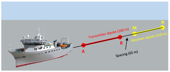
Figure 1.
Schematic layout of the towed galvanic-excitation TDEM array used for field acquisition in ESAS in 2020 [35] and synthetic modeling analysis in this study.
In the towing process, the source injects current into water, with a certain pulse duration and time delay between consecutive pulses, and once each pulse ends, the transient voltage signal is recorded. In typical Arctic shelf surveys [35], individual responses (stations) are collected every 4 s (having 1 ms sampling rate) within 2 s intervals following another 2 s current transmission phase. Depending on the vessel speed (4–10 knots), the station spacing varies from 13 to 50 m. Practically, the transmitted current value (pulse amplitude) is between 170 and 200 A and is continuously recorded along with voltage measurements with the same sampling rate.
2.2. Construction of Quasi 2D Resistivity Model Set
The initial point of this study was the construction of a set of characteristic quasi-2D resistivity models reflecting the structural features of the permafrost formation corresponding to a different setting, including the presence/absence of ice-bonded permafrost layer, different geometry of its top and bottom boundaries, different width and thickness of thawed bodies or taliks, variable seawater depth and its resistivity. This was done based on the analysis of field-data inversions employing TDEM datasets collected in ESAS in recent years [35,36]. The 2D models are effectively the collections of 1D depth-resistivity models assembled to form the images referenced with respect to the distance (0–2 km range) and depth (0–200 m). Each 1D column has a horizontal span of 25 m.
The constructed model set includes 5 models (A to E, Figure 2 and Figure 3) featuring 4 layers (top to bottom conductive seawater, less conductive unfrozen sea bottom sediments, resistive IBP and conductive sub-permafrost sediments), in which model A is a baseline reference model (Figure 2a) with the following parameters: seawater resistivity 0.3 Ohm·m, thickness varies from 5 to about 60 m; unfrozen sea bottom sediments resistivity 2 Ohm·m, thickness varies from 10 to about 70 m; homogenous IBP with resistivity of 100 Ohm·m and thickness varying between 100 and 30 m, homogenous sub-permafrost semi-infinite layer with 10 Ohm·m resistivity. Models B (Figure 2b) and C (Figure 2c) are essentially the same as model A but have lower resistivity of the IBP layer (30 Ohm·m for model B and 5 Ohm·m for model C). Model D (Figure 3b) differs from model A only in a way that its IBP thickness is doubled, while model E (Figure 3c) has the same geometry as model A, but all the resistivities (except for the sub-permafrost layer) vary smoothly in a horizontal direction to simulate variable salinity in the water layer, non-uniformity of the unfrozen seafloor sediments and the presence of thawed regions (taliks) within IBP formation.
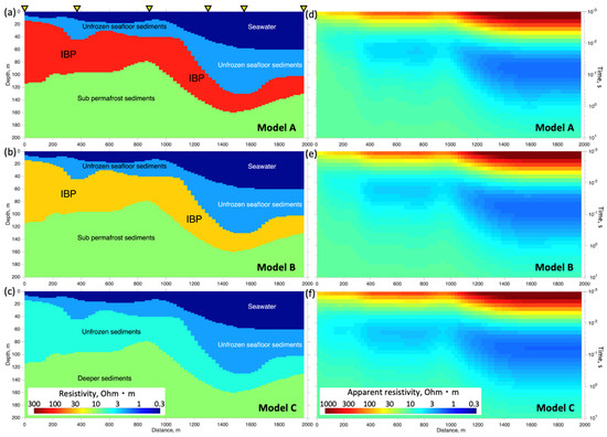
Figure 2.
Synthetic resistivity models (left-hand panels) and modeled apparent resistivity pseudo-sections (right-hand panels): (a) resistivity image for model A. Yellow inverted triangles show the locations where individual responses used in further analysis were calculated; (b) resistivity image for model B; (c) resistivity image for model C; (d) apparent resistivity pseudo-section for model A; (e) apparent resistivity pseudo-section for model B; (f) apparent resistivity pseudo-section for model C.
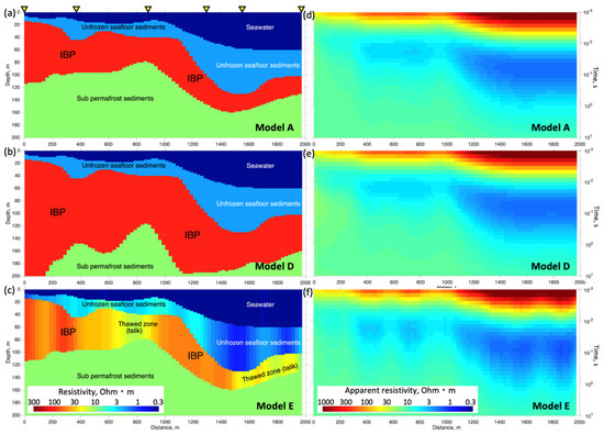
Figure 3.
Synthetic resistivity models (left-hand panels) and modeled apparent resistivity pseudo-sections (right-hand panels): (a) resistivity image for model A. Yellow inverted triangles show the locations where individual responses used in further analysis were calculated; (b) resistivity image for model D; (c) resistivity image for model E; (d) apparent resistivity pseudo-section for model A; (e) apparent resistivity pseudo-section for model D; (f) apparent resistivity pseudo-section for model E.
When interpreting the inversion results, given the equality of the models obtained, we also use conductance. For an arbitrary 1D resistivity profile, the conductance, also known as integrated conductivity, is calculated as
where is the integration variable over depth. In the case of N-layer resistivity structure, the conductance of its portion from the surface down to the bottom of the ith layer is written as
In addition to analyzing models A to E, we also generated a cloud consisting of around 105 1D 3-layer models, simulating variable combinations of resistivity and geometry parameters for the upper part of the submarine structure. These are covered in full detail in Section 3.3.
2.3. 1D Forward Modeling of Synthetic TDEM Data
The above model set was used as input data for TDEM response modeling assuming real towed dipole–dipole array configuration, employed in ESAS surveys [35] and shown in Figure 1. Both 160 m long transmitter and 150 m long receiver horizontal arrays a submerged 1 m beneath water and aligned along the towing line. Source dipole current was set at 180 A, with a pulse duration of 2 s.
Despite the substantial lateral variations seen in constructed hypothetical resistivity models, the maximum lateral station-to-station gradient is about 15–20%, and these models remain within limits, where 1D locality is expected to hold (lateral size of locality domain is nearly the same as the depth of investigation) [37]. Moreover, the models exaggerate typical contrasts found in the real setting of the Arctic shelves [35], with very smooth changes in bathymetry and subbottom geology. The above arguments justify the implementation of the fast and efficient 1D codes for TDEM response simulation and inversion instead of far more resource-consuming 2.5D software.
To calculate the 1D synthetic responses, we applied the frequency-domain DIPOLE1D code by K. Key [38] enabling high-accuracy numerical modeling of electric and magnetic field components, taking the finite source dipole length into account. Modeled frequency responses are then converted into the time domain through a convolution transform. Finally, transient responses (voltages) are obtained for each of the collections of 1D models forming 2D resistivity images shown in the left-hand panels of Figure 2 and Figure 3. Transient voltages are transformed into apparent resistivities assuming late-stage approximation [26]:
where is the transmitted current, and is the magnetic permeability of the vacuum, t is transient time since current cut-off, and AB is transmitter dipole length. Apparent resistivity pseudo-sections are the right-hand panels of Figure 2 and Figure 3.
2.4. 1D Constrained Inversion of TDEM Data
For 1D inversion of marine TDEM data, we applied the MATLAB-based TEM1DInv code (Figure 4) employing Optimization Toolbox functionality [39]. The input dataset was a combination of apparent resistivity responses, calculated earlier for models A and E, decimated to a sparser time grid and for practical reasons taken within the limited time range (1–100 ms), where field data usually have acceptable quality. A nonlinear inversion procedure [32] converts the apparent resistivity response at each station into the one-dimensional (horizontally-layered) resistivity model beneath it. The inverse problem is solved by minimizing the objective function (data misfit), defined as the normalized sum of the squared differences of the logarithms of late-stage apparent resistivities . Summation is done over the time samples on a logarithmic grid:
where ti denotes time samples with logarithmic spacing, Nt is the number of samples in a given response curve; is input synthetic data; characterize data errors (set to 1 in our synthetic experiment); is modeled response, calculated from the N-layer resistivity model m referenced to station x
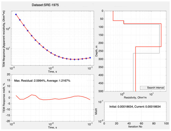
Figure 4.
Graphical user interface (GUI) of the TEM1DInv software. Upper left: input synthetic apparent resistivity (blue points) and calculated (red line) response at current iteration; upper right: initial guess (grey line) and current iteration (red line) depth-resistivity profiles; lower left: response residual between input and calculated responses.
Thus, m is a vector composed of logarithmic resistivities and thicknesses . Hence, and correspond to the water layer, whose thickness is known and resistivity is believed to vary within a relatively narrow range (Table 1). Minimization of the objective function is done with a modification of the gradient descent method, using the functionality of MATLAB’s Optimization Toolbox. In this study, we apply constrained inversion in which the model parameter search is done within the specified bounds for each constituent of model vector m, representing a 4-layer resistivity structure. These are chosen based on available data and estimates (Table 2) [12,20,35,36,40].

Table 1.
Bounds for model parameters used in 4-layer constrained inversion.
Table 2.
Three-layer model parameters’ ranges used to estimate inversion uncertainty.
An important aspect of inversion stabilization (regularization) is that seawater depth is constrained within a 10 percent margin of the known bathymetry data, estimated by averaging the ETOPO1 model and sonar data. This reduces the number of parameters being recovered and greatly facilitates inversion stability.
The code requires the initial guess (starting) model to be specified, and the profile data inversion runs successively in a way that the final model for the current station is used as the initial one for the next station along the line. The resistivity of layer 1 (seawater) is searched within 20% bounds of the initial value, calculated at each station from salinity data assuming the Practical Salinity 1978 model [41]. Further, to provide lateral smoothness of the resulting model, all parameters at each given station are constrained within a 20% margin of those at the previous station in line. The initial guess for the first station in a line is specified according to a priori data and sensitivity tests.
3. Results
Simulated apparent resistivities shown in Figure 2d–f and Figure 3d–f reveal the smoothed patterns with certain features of similarity to the true geometry of the resistivity models. However, these pseudo-sections are only the form of the response, where the vertical dimension is time, and these cannot be directly compared to the original resistivity images (panels a–c in Figure 2 and Figure 3). Nevertheless, the shape of the bluish region representing the response of the conductive portion of the model (water and unfrozen sediments), correlates with the thickness and conductivity of the upper 3 layers, including the IBP layer. The right-hand part of the pseudo-section images, corresponding to greater water depth and higher conductance of the seafloor sediments, have a larger portion of the early-time high-resistivity region (1–7 ms versus 1–3 ms time interval for a shallow-water setting), which is an indication of the fact that far-field behavior lasts longer in a less resistive environment [26].
3.1. Synthetic Study of TDEM Response Sensitivity to Permafrost Parameters in ESAS Setting
To understand the effect of specific resistivity or geometry of the IBP formation, as well as the resistivity of unfrozen sediments above and below the IBP layer, we plotted relative response anomalies as time-distance pseudo-sections in Figure 5. These were calculated from the apparent resistivity time-distance distributions shown in Figure 2 and Figure 3d–f as
where x denotes distance and t is the time passed since the current cut-off.

Figure 5.
Relative anomaly pseudo-sections, calculated from apparent resistivity data: (a) between model B and model A; (b) between model C and model A; (c) between model D and model A; (d) between model E and model A.
Despite the significant prevalence of seawater and bottom sediments’ conductances over those of the underlying IBP formation, all models show substantial anomalies relative to reference model A. Model B in which the IBP layer’s resistivity is ~3 times lower compared to model A, exhibits on average 10% negative anomaly (decreased apparent resistivity), with maximum absolute values seen at small distances (0–300 m), which is due to highest sensitivity to IBP present in this interval associated with the most shallow water layer. Model C, being essentially a no-IBP model, shows intense positive anomaly within an early time range (1–6 ms) followed by a strong negative anomaly in 7 ms−1 s intervals, with the amplitude decaying smoothly (to −5%) in the right-hand part of the plot. Inversely, Model D, having 2-fold increased IBP thickness, shows a weak −5% negative anomaly at early times, and then a clear 10–15% positive anomaly within the 10 ms−1 s time range, which gets slightly lower (around 5%) at distances greater than 1400 m. Finally, model E, being a perturbated version of model A, with resistivities varying smoothly in a lateral direction in all 3 upper layers, shows a mosaic pattern of the time-distance anomaly distribution, which is consistent with alternating series of increased and decreased resistivity regions. In terms of time distribution, the response shows coupled positive and negative anomalies which is the indication of change in the slope of the early-time apparent resistivity curve segment relative to the reference (model A).
Individual responses extracted at 6 specific locations are shown in Figure 6. It can be seen that in a shallow-water setting, all 5 models differ significantly in terms of response curve shape in the time range of 10 to 100 ms (Figure 6a–c). However, those differences become much smaller in the deep-water environment (Figure 6d–f). Despite the upper layer being a conductor, the behavior displayed by the responses clearly indicates the prevalence of the far-field descending segment within the initial time range between 1 ms and 3–10 ms, depending on the local model, i.e., the conductance of the upper formation. Response minima, associated with the conductive layer(s), are typically observed at around 6–10 ms (x = 0 m), 10–20 ms (x = 350; 875 m) and 40–60 ms (x = 1300; 1575; 1975 m), which correlates with the increase in the formations’ thickness towards the greater distances. The minimum value varies between around 10 and 1.5 Ohm·m, consistently getting lower towards the right-hand part of the profile with a conductance increase. Locations x = 0, 350 and 875 m naturally exhibit significant differences between the responses corresponding to Models A–E (location x = 0 shows the largest anomalies, of about 30% within the intermediate time range), which is indicative of high sensitivity to subbottom structure in a shallow-water setting. Oppositely, a deeper-water setting (x = 1300, 1575 and 1975 m) implies much smaller misfits (not exceeding a few percent) between various curves, except for Model E at x = 1575 and 1975 m, which clearly deviates from other responses due to substantial differences in conductivity of water, seafloor sediments and IBP formation.

Figure 6.
Synthetic apparent resistivity responses calculated for 6 specific locations along the simulated profile (shown as yellow inverted triangles in Figure 2a and Figure 3a). Different colors correspond to different synthetic models (A to E): (a) location 0 m, shallow water, thin unfrozen seafloor layer, thicker IBP setting; (b) location 350 m, shallow water, thicker unfrozen seafloor layer, thinner IBP setting; (c) location 875 m, setting is similar to that in (b); (d) location 1300 m, seafloor slope, water thickness is nearly equal to that of unfrozen seafloor layer (about 40 m each), deeper and thinner IBP setting; (e) location 1575 m, deep-water (60 m) setting, increased thickness of unfrozen seafloor layer (about 70 m), deeper and thinner IBP formation; (f) location 1975 m, deep-water (60 m) setting, 40 m unfrozen seafloor layer, shallower and thinner IBP formation.
3.2. Inversion of the Synthetic Responses
In order to understand the practical capabilities and limitations of the galvanic excitation-based TDEM technology in the marine environments for IBP mapping, we applied 1D inversion code to synthetic apparent resistivity datasets calculated for models A and E. The resulting resistivity images in comparison with true models along with misfit pseudo-sections are presented in Figure 7 and Figure 8.

Figure 7.
Synthetic data inversion results for model A: (a) true model resistivity image; (b) inverted model resistivity image. Dashed lines show the true geometry of layer boundaries: seafloor (bottom of layer 1, white dashed line, fixed during inversion), top and bottom of the IBP formation (black dashed lines, layer 3, free during inversion); (c) relative data error pseudo-section for the last iteration. Green color indicates better fit.
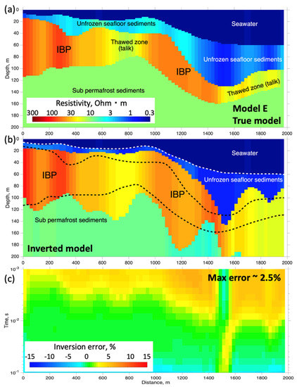
Figure 8.
Synthetic data inversion results for model E: (a) true model resistivity image; (b) inverted model resistivity image. Dashed lines show the true geometry of layer boundaries: seafloor (bottom of layer 1, white dashed line, fixed during inversion), top and bottom of the IBP formation (black dashed lines, layer 3, free during inversion); (c) relative data error pseudo-section for the last iteration. Green color indicates better fit.
Both inverted models show reasonable consistency with the original (true) models, and major resistivity features have been successfully recovered. However, some model elements show erroneous configurations, which is mainly attributed to the underestimated thickness and resistivity of layer 2 (relatively conductive unfrozen seafloor sediments), causing the top of IBP to be mapped with depth error from a few meters in a shallow-water setting to 40 m in a deep-water environment, causing the reduction in sensitivity to the underlying structure. In Figure 9, we evaluate the quality of the inverted models in terms of how they fit the true conductances calculated for individual layers 2 and 3, as well as the total conductance of layers 1 and 2. From the graphs, it can be easily seen that seawater’s (layer 1) conductance (20 to 200 S) is substantially higher than that of the seafloor unfrozen sediments (layer 2, 5–60 S) and largely prevails (by) over conductance of the IBP formation (layer 3, 0.2–2 S). Despite showing substantial errors in layer 2’s thickness and resistivity, the results for both models A and B exhibit a precise fit in terms of combined conductivity of seawater and unfrozen sea bottom sediments (green line indicates the true distribution, and the dotted one corresponds to inversion), which is in agreement with conductance equivalence known for inductive EM methods [26].

Figure 9.
Conductance profiles for the true (solid lines) and inverted (dotted lines) models calculated for individual layers 1, 2 and 3 (black, blue and red lines, respectively), as well as grouped layers 1 and 2 (green line): (a) graphs for model A; (b) graphs for model E.
The most prominent feature of the inverted models is accurate (to within a few percent) recovery of summated conductance of the seawater, layer 1, and unfrozen bottom sediments, layer 2 (green dotted and solid lines in Figure 9 show good fit quality), while the recovered conductance of the layer 2 alone is slightly less accurate (blue line and dots) which is natural due to much lower conductance compared to seawater. Finally, target layer 3 shows the worst conductance fit quality, with errors reaching 5–10 fold of the true value, which generally increases from left to right as the conductance of the overlying formations increases from nearly 20 to over 200 S.
Obviously, this behavior is in agreement with the conductance equivalence principle stating that the recorded decay response is effectively controlled by the total conductance of the upper conductive strata, rather than by individual resistivities and thicknesses of its layers, assuming near-field approximation [26]. Thus, even if the seawater resistivity and thickness are constrained by directly-measured salinity and bathymetry data, given the non-zero bias present in the response, the inversion targeted at mapping the IBP’s top boundary (i.e., the thickness of relatively conductive subbottom sediments) remains non-unique within the conductance-equivalent bounds. Nevertheless, it enables estimating its conductance with reasonable accuracy, which can be used further to constrain thickness if resistivity estimates are available from drilling or seafloor sampling. Conductance can also be used in coupled resistivity—heat transfer modeling through additional constraints.
In Models A and E, the true conductance of the IBP layer is 20 to 800 times lower than that of the overlying formation (including seawater); however, it still has an effect on calculated responses and is reliably and smoothly imaged by the inversion. In Model E inversion results (Figure 8b), both talik zones with reduced resistivity located within distance intervals of 700–900 and 1500–2000 m, respectively, have been imaged by the inverted model.
3.3. Estimating Inversion Uncertainty for TDEM Stations Collected in Shallow-Water and Deep-Water Setting
Given the seawater depth range in ESAS varies from 10 to 100 m, and its typical resistivity value is around 0.3 Ohm·m), the conductance estimates fall between 30 and 300 S, which means that in order to be discriminated by the data, any features of interest in the underlying portion of the section must have a conductance of at least 20–30% of the conductance of overlying layers. Obviously, this implies a rapid decrease in subbottom sensitivity associated with an increase in seawater depth, a factor that mainly controls its conductance.
To estimate and illustrate the effect of sensitivity and inversion uncertainty (equivalent solutions) for the subbottom part of the resistivity structure under various noise settings, we have calculated the response dataset including over 100 k transient curves corresponding to a set of 1D 3-layer models with variable resistivities and thicknesses. The model includes the water layer (resistivity 0.25–0.6 Ohm·m, thickness 10–70 m), bottom sediments (resistivity 1–1000 Ohm·m, thickness 10–1000 m) and a deeper semi-infinite layer (resistivity 1–1000 Ohm·m); see Table 2 for details. All possible combinations of parameter values varying within the above ranges produce a series of models, and a dataset of transient response curves, the latter is shown as a grey-colored cloud in Figure 10. Among those, we have chosen two particular models/response curves, that imitate resistive permafrost (500 Ohm·m) overlaid by thawed bottom sediments and water, differing in water depth (15/60 m), water resistivity (0.4/0.3 Ohm·m), bottom sediment thickness (15/30 m) and resistivity (2/5 Ohm·m). Response for the shallower water model (15 m) is shown in Figure 10 as a red dotted curve, while the one for deeper water (60 m) is indicated as blue points. Those two configurations simulate two different settings, characteristic of the most shallow part of the Laptev shelf (Bour Khaya Gulf), with less saline (and more resistive) water due to freshwater inflow from the Lena delta, and outer part of the shelf, with higher depth (ranging from 50 to 100 m and more) further to the north.

Figure 10.
Synthetic TDEM responses computed for series of 3-layer 1D models with variable resistivities and thicknesses (grey curve cloud, see Table 2 for model parameters). (a) Transient voltages; (b) apparent resistivities. Red and blue dotted curves correspond to shallow-water and deep-water models, respectively.
We calculated the misfits between each of these responses and each of all the responses forming the test dataset (grey cloud in Figure 10, numbered by j) as
where is either “shallow water” or “deep water” transient response, is jth response from a complete simulated dataset, and denote time samples, counting from 1 to . Based on misfit values obtained, we categorized all the models into 4 groups, so that corresponding responses fit curves to within 10, 5, 2 or 1 percent error (averaged over the curve).
Figure 11 illustrates the margins of each category in model space, shown as red, blue, green and red regions, respectively, for 10%, 5%, 2% and 1% data error for each of two specific responses, “shallow-water” (Figure 11a) and “deep-water” (Figure 11b). One obvious conclusion is that a shallow-water setting results in a narrower resistivity range for layers 2 and 3, being of primary interest when resolving the structure in terms of lower resistivity (thawed sediments) or higher resistivity (frozen sediments). In most cases, 1%, 2%, 5% and 10% data errors are all acceptable to enable discriminating between the lower (less than 10 Ohm·m) and higher (more than 10 Ohm·m) resistivity in both layers 2 and 3; 1% data accuracy shows more certain inversion bounds (yellow).
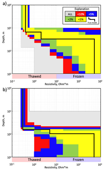
Figure 11.
Inverted model uncertainty plots. (a) Model set for “shallow-water” responses; (b) model set for “deep-water” responses. Colored regions show model space domains containing all models whose responses fit the simulated response (in data space) to within a specified misfit level: 10% (red), 5% (blue), 2% (green) and 1% (yellow). Grey region shows the margins of all models generated in this test. Solid black lines indicate the true models for either case.
In the case of a deep-water setting, the resistivity bounds for 10% and 5% data error are less definitive (Figure 11b) compared to shallow water, which indicates a severe lack of sensitivity to deeper layers’ resistivities. Though 2% and 1% margins still exhibit some moderate sensitivity to the layer 3 resistivity, the measured transient time given is large enough. Note that intermediate layer 2, given its relatively small thickness, is resolved with the largest uncertainty. The above analysis shows the limitations of TDEM inversion precision, pointing to the necessity of high data quality, while in practice keeping the data error within a 2% threshold seems to be problematic, specifically in a late transient time range.
4. Discussion
Permafrost studies, unfolding in recent years on the Arctic shelves, require a reasonably accurate mapping tool, capable of imaging the sedimentary structure down to 200–300 m depth. Although TDEM has been employed for decades in a broad set of environments and applications [25], and its capabilities and limitations are quite well understood [20], this tool remains somewhat exotic in a marine setting. The marine environment implies a strong effect of the saline low-resistivity water layer and water-saturated seafloor sediments obscuring the resistivity structure beneath. Successful implementation of marine TDEM-based systems in deep-ocean environments has been achieved through the employment of submerged source–receiver arrays towed relatively close to the seabed [42,43], or receivers deployed on the seafloor [34], or remotely operated vehicles carrying loop-based instruments [30]. Another approach, promoted by Barsukov and Fainberg [29], is based on vertical electric field measurements, carried out by a dipping receiver towed behind a horizontal dipole source. Locating the transmitter and receiver closer to the seafloor is obviously beneficial in terms of EM response sensitivity, however is costly and performance-limiting, while the present day large-area shallow-water surveys require fast and cheap solutions.
TDEM applications in permafrost studies remain quite limited compared to other fields, such as hydrocarbons and mineral exploration. Yet, since the 1980s there have been attempts to use TDEM for permafrost mapping, along with an investigation of its efficiency. The thesis by G.G. Walker [44] extensively covers practical ground-based TDEM data collected in Alaska with a loop system. From apparent resistivity responses measured mainly within 10−4 to 10−2 s time intervals, by making use of a 1D inversion code, resistivity models have been obtained, showing a resistive permafrost layer with a thickness ranging up to 600 m. A synthetic study [45] also simulating an onshore permafrost setting, found the ability of TDEM response to image lateral inhomogeneities both in permafrost geometry and resistivity of the conductive sediments beneath IBP.
Under typical onshore conditions, with a large-thickness high-resistivity top layer, TDEM data tend to display rapid decay immediately from the early transient time (100 mcs), making it hard to achieve measurable signal at late times (around 1 s), though remain sensitive to conductive formation beneath the resistive layer. On the opposite, in the case of subsea permafrost, the common setting involves low-resistivity layer(s) above the higher-resistivity target structure.
Despite the availability of some amount of onshore resistivity studies, to our knowledge, examples of marine TDEM permafrost studies are rare. Ice-based, yet marine, TDEM measurements taken in shallow (a few meters) waters near Muostakh Island (the coastal part of the Laptev Sea) [36] yielded IBP thickness estimates of nearly 500 m; however, these were loop soundings along the relatively short line with significant spatial separations between the stations.
The recent TDEM onshore loop-system survey by Creighton et al. [46] revealed a nearly 100 m thick low-resistivity (1–2 Ohm·m) talik beneath a thermokarst lake in Alaska, with an overall imaging depth of 200 m and no signs of IBP bottom boundary within this depth range (the IBP is likely much thicker in this area). This resistivity-thickness configuration of the conductive top layer (50 to 100 S in terms of conductance) is roughly equivalent to a marine setting with water depth ranging from 15 to 50 m and water resistivity varying between 0.3 and 0.5 Ohm·m. In the above study TDEM was capable to image resistive (tens Ohm·m) IBP beneath the talik, and, although a different array configuration was used, it is still fairly close to the one we use in our analysis in terms of depth of investigation and sensitivity.
Our dipole–dipole TDEM data from Laptev Sea collected in 2020 in the area with seawater depth varying between 7 and 15 m, and water resistivity between 0.47 and 0.55 Ohm·m, reveal relatively uniform permafrost layer having a thickness of 100–200 m, and distinctive sensitivity to sub-permafrost conductive sediments [35], thus proving the technology efficacy in a shallow-water setting. Notably, the IBP thickness estimates obtained from inverted TDEM data turn out to be substantially lower compared to existing temperature-based models for this area [10].
Thus, in this study we focus on a specific setting involving a marine towed dipole–dipole TDEM system, relatively shallow saline water covering subbottom sedimentary formations which may host a laterally non-homogenous permafrost layer, and apply the numerical study to evaluate the method’s sensitivity and inversion uncertainty to specific properties of the submarine IBP layer and overlying unfrozen sediments, assuming 1D approximation.
Synthetic data analysis included the inversion of simulated response data within a limited time range (1–100 ms, usually available with acceptable quality from the survey data) with constraints imposed on seawater parameters (these are known from bathymetry and salinity data) to evaluate the uncertainty of recovered resistivity images under conditions typical for ESAS environments with variable water depth and IBP characteristics.
Inversion of the response dataset calculated for the model having laterally-variable layer resistivity, including low-resistivity talik regions within the IBP formation (Model E), shows reasonable accuracy and proves the method’s ability to discriminate taliks from intact IBP, except for a particular zone (x = 1500–1600 m), where an overlying structure has conductance over 250 S.
Evaluation of model equivalence bounds based on compiling a large response set assuming the 3 layer structure (water, unfrozen sediments, permafrost) and calculating misfits with the true response, suggests the sufficient accuracy of the model recovery, given the data errors are within 1% threshold over the 1–1000 ms time range, allowing for discrimination between thawed (<10 Ohm·m) and frozen (>10 Ohm·m) states (yellow region in Figure 11) of the basement (permafrost) layer. However, available ESAS survey data usually exhibit substantially higher errors [47], while a 5% error floor is obviously not enough for such discrimination (blue region in Figure 11), especially in deep-water settings.
One of the crucial problems is connected with response distortions [48], mainly presenting as low-frequency bias that leads to a significant shortening of interpretable segments of measured responses, in turn causing the reduction of DOI.
Thus, TDEM acquisition/inversion technique yields large amounts of high-resolution data enabling in situ probing of permafrost thickness and lateral distribution aiming at a better understanding of the extent of the IBP formation in the study area. The peculiarities of transient EM field behavior observed from synthetic data determine the method’s capabilities depending on sea bottom depth, as well as resistivity features of the subbottom structure. Indeed, deeper water results in reduced DOI and sensitivity of TDEM response to the portion of section beneath the seafloor. Provided that transmitter and receiver are placed at the water surface (or slightly submerged), the high conductance of the seawater may play the dominant role, obscuring (or screening) the underlying formations so that the response curve becomes less sensitive to their parameters.
5. Conclusions
We carried out a modeling-based analysis of the towed dipole–dipole TDEM system capabilities with respect to subsea permafrost imaging. In compiling the synthetic resistivity models, we relied on known permafrost-related resistivity patterns [12,20,40] as well as survey data on the bathymetry, water salinity and previous EM studies in the ESAS region [31,35,36]. The study included forward modeling TDEM data (response) analysis for five synthetic models simulating different settings (presence/absence of ice-bonded permafrost layer, different positions of its top and bottom boundaries, different width and thickness of thawed bodies or taliks, variable sea-water depth and its resistivity), inversion of response for particular models and estimation of the inversion uncertainty for shallow-water and deep-water setting.
From the comparison of the modeled responses, it can be seen that the models can be essentially discriminated between each other despite the significant prevalence of the effect of seawater and unfrozen sediments, with all 5 models differing significantly in terms of response curve shape in time range 10 to 100 ms, except for the deep-water portion (water depth over 50 m), where this difference becomes smaller.
Inversion results are found to reproduce the main features of the true models, although the thickness of relatively conductive unfrozen seafloor sediments has some tendency to underestimation. Inverted images show accurate (to within a few percent) recovery of summated conductance of the seawater and unfrozen bottom sediments, while the recovered conductance of the latter alone is slightly less accurate. Finally, the target IBP shows lower conductance fit quality, which generally increases following the increase in conductance of the overlying formations. Nevertheless, talik zones with reduced resistivity have been imaged by the inversion, and IBP conductance still can be estimated with reasonable accuracy. Conductance estimates can be used further to constrain thickness if resistivity estimates are available from drilling or seafloor sampling, and also might be helpful in coupled resistivity—heat transfer modeling through additional constraints.
An uncertainty study involving multiple 1D 3-layer models suggests that the shallow-water (10–20 m) setting results in narrower resistivity ranges for target layers when resolving the structure in terms of lower resistivity (thawed sediments) or higher resistivity (frozen sediments). In most cases discrimination between lower (less than 10 Ohm·m) and higher (more than 10 Ohm·m) resistivity is possible. Deep-water setting (30–70 m) yields a substantial lack of sensitivity to deeper layers’ resistivities. However, the 2% response error margin still exhibits some moderate sensitivity to the lower layer resistivity, given the measured transient time is large enough.
The above analysis shows the limitations of TDEM inversion precision, pointing to the necessity of high data quality, namely, keeping the data error within the 2–3% threshold, especially in deep-water settings.
This study allowed us to understand the possible uncertainties in the geometry and resistivity of the reconstructed permafrost layer, depending on seawater depth and unfrozen layer thickness, and confirm the overall efficacy of TDEM technology for the subsea permafrost imaging, which is crucially important for understanding the current state of the subsea permafrost-hydrate system and possible future dynamics. Furthermore, the obtained modeling results can be used to modify and improve the technology for collecting permafrost mapping data in the ESAS.
Author Contributions
Conceptualization, D.A.A. and A.V.K.; methodology, D.A.A., A.V.K. and N.A.P.; investigation, D.A.A., A.V.K., A.Y.G., E.I.B. and N.E.S.; resources, A.V.K., A.Y.G. and E.I.B.; data curation, D.A.A., A.Y.G. and E.I.B.; writing—original draft preparation, D.A.A. writing—review and editing, all authors; visualization, D.A.A. and E.I.B.; supervision, A.V.K., L.I.L. and I.P.S.; project administration, L.I.L. and I.P.S.; funding acquisition, I.P.S. All authors have read and agreed to the published version of the manuscript.
Funding
This research was funded by Tomsk State University Russian Federation (Project ‘Prioritet-2030’) (study design, model creation) with partial support from the Russian Science Foundation, (Projects no. 21-77-30001, code development, and 22-67-00025, data analysis) and P.P. Shirshov Institute of Oceanology under State Assignment (Project No. FMWE-2021-0005) (numerical modeling, visualization). Authors are also grateful for support from the Russian Ministry of Science and Education (grant 021-2021-0010) for opportunity for the testing experiments at the sea.
Conflicts of Interest
The authors declare no conflict of interest.
References
- Arctic Climate Impact Assessment. ACIA Overview Report; Cambridge University Press: Cambridge, UK, 2005; 1020p. [Google Scholar]
- Soloviev, V.A. Gas-hydrate-prone areas of the ocean and gas-hydrate accumulations. In Proceedings of the Sixth International Conference on Gas in Marine Sediments, St. Petersburg, Russia, 5–9 September 2000. [Google Scholar]
- Shakhova, N.E.; Semiletov, I.P. Methane hydrate feedbacks. In Arctic Climate Feedbacks: Global Implications; Sommerkorn, M., Hassol, S.J., Eds.; WWF International Arctic Programme August: Solna, Sweden, 2009; pp. 81–92. [Google Scholar]
- Shakhova, N.; Semiletov, I.; Chuvilin, E. Understanding the permafrost–hydrate system and associated methane releases in the East Siberian Arctic Shelf. Geosciences 2019, 9, 251. [Google Scholar] [CrossRef]
- Kvenvolden, K.A.; Lilley, M.D.; Lorenson, T.D.; Barnes, P.W.; McLaughlin, E. The Beaufort Sea continental shelf as a seasonal source of atmospheric methane. Geophys. Res. Lett. 1993, 20, 2459–2462. [Google Scholar] [CrossRef]
- Semiletov, I.P.; Pipko, I.I.; Pivovarov, N.Y.; Popov, V.V.; Zimov, S.A.; Voropaev, Y.V.; Daviodov, S.P. Atmospheric carbon emissions from northern lakes: A factor of global significance. Atmos. Environ. 1996, 30, 1657–1671. [Google Scholar] [CrossRef]
- Shakhova, N.; Semiletov, I.; Salyuk, A.; Joussupov, V.; Kosmach, D.; Gustafsson, O. Extensive methane venting to the atmosphere from sediments of the East Siberian Arctic Shelf. Science 2010, 327, 1246–1250. [Google Scholar] [CrossRef] [PubMed]
- Shakhova, N.; Semiletov, I.; Leifer, I.; Sergienko, V.; Salyuk, A.; Kosmach, D.; Chernikh, D.; Stubbs, C.; Nicolsky, D.; Tumskoy, V.; et al. Ebullition and storm-induced methane release from the East Siberian Arctic Shelf. Nat. Geosci. 2014, 7, 64–70. [Google Scholar] [CrossRef]
- Shakhova, N.; Semiletov, I.; Sergienko, V.; Lobkovsky, L.; Yusupov, V.; Salyuk, A.; Salomatin, A.; Chernykh, D.; Kosmach, D.; Panteleev, G.; et al. The East Siberian Arctic Shelf: Towards further assessment of permafrost-related methane fluxes and role of sea ice. Phil. Trans. R. Soc. 2015, 373, 20140451. [Google Scholar] [CrossRef]
- Romanovskii, N.N.; Kholodov, A.L.; Gavrilov, A.V.; Tumskoy, V.E.; Hubberten, H.W.; Kassens, H. Thickness of ice-bonded permafrost in the eastern part of the Laptev Sea shelf. Earth Cryosphere 2003, 65–75. [Google Scholar]
- Nicolsky, D.J.; Romanovsky, V.E.; Romanovskii, N.N.; Kholodov, A.L.; Shakhova, N.E.; Semiletov, I.P. Modeling sub-sea permafrost in the East Siberian Arctic Shelf: The Laptev Sea region. J. Geophys. Res. 2012, 117, F03028. [Google Scholar] [CrossRef]
- Piskunova, E.A.; Palshin, N.A.; Yakovlev, D.V. Electrical conductivity features of the Arctic shelf permafrost and electromagnetic technologies for their studies. Russ. J. Earth Sci. 2018, 18, ES5001. [Google Scholar] [CrossRef]
- Du Frane, W.L.; Stern, L.A.; Constable, S.; Weitemeyer, K.A.; Smith, M.M.; Roberts, J.J. Electrical properties of methane hydrate + sediment mixtures. J. Geophys. Res. Solid Earth 2015, 120, 4773–4783. [Google Scholar] [CrossRef]
- Waite, W.F.; Santamarina, J.C.; Cortes, D.D.; Dugan, B.; Espinoza, D.N.; Germaine, J.; Jang, J.; Jung, J.W.; Kneafsey, T.J.; Shin, H.; et al. Physical properties of hydrate-bearing sediments. Rev. Geophys. 2009, 47, RG4003. [Google Scholar] [CrossRef]
- Overduin, P.P.; Westermann, S.; Yoshikawa, K.; Haberlau, T.; Romanovsky, V.; Wetterich, S. Geoelectric observations of the degradation of nearshore submarine permafrost at Barrow (Alaskan Beaufort Sea). J. Geophys. Res. 2012, 117, F02004. [Google Scholar] [CrossRef]
- Angelopoulos, M.; Westermann, S.; Overduin, P.P.; Faguet, A.; Olenchenko, V.; Grosse, G.; Grigoriev, M.N. Heat and salt flow in subseapermafrost modeled withCryoGRID2. J. Geophys. Res. Earth Surf. 2019, 124, 920–937. [Google Scholar] [CrossRef]
- Angelopoulos, M.; Overduin, P.P.; Jenrich, M.; Nitze, I.; Günther, F.; Strauss, J.; Westermann, S.; Schirrmeister, L.; Kholodov, A.; Krautblatter, M.; et al. Onshore thermokarst primes subsea permafrost degradation. Geophys. Res. Lett. 2021, 48, e2021GL093881. [Google Scholar] [CrossRef]
- Hauck, C.; Mühll, D.V.; Maurer, H. Using DC Resistivity Tomography to detect and characterize mountain permafrost. Geophys. Prosp. 2003, 51, 273–284. [Google Scholar] [CrossRef]
- Arboleda-Zapata, M.; Angelopoulos, M.; Overduin, P.P.; Grosse, G.; Jones, B.M.; Tronicke, J. Exploring the capabilities of electrical resistivity tomography to study subsea permafrost. Cryosphere 2022, 16, 4423–4445. [Google Scholar] [CrossRef]
- Kawasaki, K.; Osterkamp, T.E. Mapping shallow permafrost by electromagnetic induction—Practical considerations. Cold Reg. Sci. Technol. 1988, 15, 279–288. [Google Scholar] [CrossRef]
- Constable, S. Review paper: Instrumentation for marine magnetotelluric and controlled source electromagnetic sounding. Geophys. Prosp. 2013, 61 (Suppl. S1), 505–532. [Google Scholar] [CrossRef]
- Sherman, D.; Kannberg, P.; Constable, S. Surface towed electromagnetic system for mapping of subsea Arctic permafrost. Earth Planet. Sci. Lett. 2017, 460, 97–104. [Google Scholar] [CrossRef]
- Constable, S.C.; Kannberg, P.; Weitemeyer, K.A. Vulcan: A deep-towed CSEM receiver. Geochem. Geophys. Geosyst. 2016, 17, 1042–1064. [Google Scholar] [CrossRef]
- Palshin, N.A. Problems of marine electromagnetic soundings. Geophys. J. 2009, 31, 78–92. [Google Scholar]
- Nabighian, M.; Macnae, J. Time domain electromagnetic prospecting methods. In Electromagnetic Methods in Applied Geophysics; Nabighian, M., Ed.; Society of Exploration Geophysicists: Tulsa, OK, USA, 1991; Volume 2, pp. 427–514. [Google Scholar]
- Kaufman, A.A.; Alekseev, D.; Oristaglio, M. Principles of Electromagnetic Methods in Surface Geophysics, 1st ed.; 45, Methods in Geochemistry and Geophysics Series; Elsevier: Amsterdam, The Netherlands, 2014. [Google Scholar]
- Christiansen, A.V.; Auken, E.; Sørensen, K. The transient electromagnetic method. In Groundwater Geophysics; Kirsch, R., Ed.; Springer: Berlin/Heidelberg, Germany, 2006. [Google Scholar]
- Giannino, F.; Leucci, G. Electromagnetic Methods in Geophysics: Applications in GeoRadar, FDEM, TDEM, and AEM; Wiley: Hoboken, NJ, USA, 2021. [Google Scholar]
- Barsukov, P.O.; Fainberg, E.B. Transient marine electromagnetics in shallow water: A sensitivity and resolution study of the vertical electric field at short ranges. Geophysics 2014, 79, E39–E49. [Google Scholar] [CrossRef]
- Nakayama, K.; Saito, A. Practical marine TDEM systems using ROV for the ocean bottom hydrothermal deposits. In Proceedings of the 2016 Techno-Ocean (Techno-Ocean), Kobe, Japan, 6–8 October 2016; pp. 643–647. [Google Scholar]
- Shakhova, N.; Semiletov, I.; Gustafsson, O.; Sergienko, V.; Lobkovsky, L.; Dudarev, O.; Tumskoy, V.; Grigoriev, M.; Mazurov, A.; Salyuk, K.; et al. Current rates and mechanisms of subsea permafrost degradation in the East Siberian Arctic Shelf. Nat. Commun. 2017, 8, 15872. [Google Scholar] [CrossRef] [PubMed]
- Zhdanov, M.S. Geophysical inverse theory and regularization problems. In Methods in Geochemistry and Geophysics Series; Elsevier: Amsterdam, The Netherlands, 2002; Volume 36. [Google Scholar]
- Nakayama, K.; Saito, A. Marine time-domain electromagnetic technologies using ROV. Geophys. Explor. 2011, 64, 255–266. [Google Scholar]
- Constable, S. Ten years of marine CSEM for hydrocarbon exploration. Geophysics 2010, 75, 75A67–75A81. [Google Scholar] [CrossRef]
- Krylov, A.A.; Ananiev, R.A.; Chernykh, D.V.; Alekseev, D.A.; Balikhin, E.I.; Dmitrevsky, N.N.; Novikov, M.A.; Radiuk, E.A.; Domaniuk, A.V.; Kovachev, S.A.; et al. A Complex of Marine Geophysical Methods for Studying Gas Emission Process on the Arctic Shelf. Sensors 2023, 23, 3872. [Google Scholar] [CrossRef]
- Koshurnikov, A.V.; Tumskoy, V.E.; Shakhova, N.E.; Sergienko, V.I.; Dudarev, A.Y.; Gunar, O.V.; Pushkarev, P.Y.; Semiletov, I.P.; Koshurnikov, A.A. The first ever application of electromagnetic sounding for mapping the submarine permafrost table on the Laptev Sea. Dokl. Earth Sci. 2016, 469, 860–863. [Google Scholar] [CrossRef]
- Barsukov, P.O.; Fainberg, E.B. On the locality of transient electromagnetic soundings with a single-loop configuration. Izv. Phys. Solid Earth 2018, 54, 349–358. [Google Scholar] [CrossRef]
- Key, K. 1D inversion of multicomponent, multi-frequency marine CSEM data: Methodology and synthetic studies for resolving thin resistive layers. Geophysics 2009, 74, F9–F20. [Google Scholar] [CrossRef]
- The MathWorks, Inc. MATLAB and Optimization Toolbox Release 2020b; The MathWorks, Inc.: Natick, MA, USA, 2020. [Google Scholar]
- Osterkamp, T.E. Sub-Sea Permafrost, Encyclopedia of Ocean Sciences, 2nd ed.; Elsevier: Amsterdam, The Netherlands, 2001; pp. 559–569. [Google Scholar]
- Lewis, E.L.; Perkin, R.G. The practical salinity scale 1978: Conversion of existing data. Deep Sea Res. Part A Oceanogr. Res. Pap. 1981, 28, 307–328. [Google Scholar] [CrossRef]
- Johnson, C.D.; Valder, J.F.; White, E.A.; Maurya, P.K.; Hisz, D.; Lane, J.W. Application of a towed time-domain electromagnetic (tTEM) imaging system in Jamestown, North Dakota. In Proceedings of the Symposium on the Application of Geophysics to Engineering and Environmental Problems, Portland, OR, USA, 17–21 March 2019; Environmental & Engineering Geophysical Society: Denver, CO, USA, 2019; pp. 322–325. [Google Scholar] [CrossRef]
- Su, Z.; Tao, C.; Shen, J.; Zhu, Z.; Nie, Z. Marine Transient Electromagnetic Exploration of Seafloor Massive Sulfide Deposits on Southwest Indian Ridge. In Proceedings of the 82nd EAGE Annual Conference & Exhibition, Online, 18–21 October 2021; EAGE: Bunnik, The Netherlands, 2021; pp. 1–5. [Google Scholar]
- Walker, G.G. Transient Electromagnetics for Permafrost. Ph.D. Thesis, University of Alaska, Fairbanks, AK, USA, December 1988; 292p. Available online: https://scholarworks.alaska.edu/bitstream/handle/11122/9354/Walker_G_1988.pdf?sequence=1 (accessed on 30 April 2023).
- Buddo, I.; Misyurkeeva, N.; Shelokhov, I.; Chuvilin, E.; Chernikh, A.; Smirnov, A. Imaging Arctic Permafrost: Modeling for Choice of Geophysical Methods. Geosciences 2022, 12, 389. [Google Scholar] [CrossRef]
- Creighton, A.L.; Parsekian, A.D.; Angelopoulos, M.; Jones, B.M.; Bondurant, A.; Engram, M.; Lenz, J.; Overduin, P.P.; Grosse, G.; Babcock, E.; et al. Transient electromagnetic surveys for the determination of talik depth and geometry beneath thermokarst lakes. J. Geophys. Res. Solid Earth 2018, 123, 9310–9323. [Google Scholar] [CrossRef]
- Goncharov, A.A.; Alekseev, D.A.; Koshurnikov, A.V.; Gunar, A.Y.; Semiletov, I.P.; Pushkarev, P.Y. Using pseudo-random code sequences for improving the efficiency of near-field transient electromagnetic sounding on the Arctic shelf. Izv. Phys. Solid Earth 2022, 58, 744–754. [Google Scholar] [CrossRef]
- Yegorov, I.V.; Palshin, N.A. Excitation of electrokinetic effects at the shallow bottom by surface waves. Oceanology 2015, 55, 417–424. [Google Scholar] [CrossRef]


Disclaimer/Publisher’s Note: The statements, opinions and data contained in all publications are solely those of the individual author(s) and contributor(s) and not of MDPI and/or the editor(s). MDPI and/or the editor(s) disclaim responsibility for any injury to people or property resulting from any ideas, methods, instructions or products referred to in the content. |
© 2023 by the authors. Licensee MDPI, Basel, Switzerland. This article is an open access article distributed under the terms and conditions of the Creative Commons Attribution (CC BY) license (https://creativecommons.org/licenses/by/4.0/).