Low-Cost Real-Time Water Level Monitoring Network for Falling Water River Watershed: A Case Study

Abstract

Streamflow monitoring for flood warning and watershed management applications in the United States is a cost-intensive venture, and usually performed by government agencies such as the US Geological Survey (USGS). With reduced resources across the federal agencies towards environmental monitoring, agencies and stakeholders are challenged to respond with cross-cutting, collaborative, and low-cost alternatives for streamflow monitoring. One such alternative is using low-cost environmental sensors and developing a real-time gage/sensor network using IoT (Internet of Things) devices. With this technology, smaller watersheds (e.g., HUC-8 and HUC-10 level) can be equipped with low-cost gages at many locations and a clear picture of the hydrological response can be obtained. This paper presents the development and implementation of a low-cost real-time water monitoring network for the Falling Water River (FWR) watershed in the middle Tennessee region in the US. To develop and implement this gage network, the following three tasks were performed: (i) assemble a low-cost, real-time internet enabled water level gage, (ii) field-test the sensor prototype and, (iii) deploy the sensors and build a network. A collaborative partnership was developed with stakeholders including the Tennessee Department of Environment and Conservation, Tennessee Department of Transportation, Burgess Falls State Park, City of Cookeville, and Friends of Burgess Falls. The performance of the gages in water level estimation was compared with the water levels measured with a nearby USGS streamgage. The comparison was performed for the 2020–2022 time period and at two levels: event-based comparison and a long-term comparison. Nine storm events were selected for the comparison, which showed “Very Good” agreement in terms of Coefficient of Determination (R²), Nash–Suttcliffe Efficiency (NSE), and percent bias (PBIAS) (except for four events). The mean squared error (MSE) ranged between 0.07 and 1.06 while the root mean squared error (RMSE) ranged between 3 inches and 12 inches. A long-term comparison was performed using Wilcoxon Signed-Rank test and Loess Seasonal Decomposition analysis, which showed that the differences between the two datasets is not significant and that they trended well across the two year period. The gages are currently installed along the main channel and tributaries of the Falling Water River, which also include portions of the Window Cliffs State Natural Area. With continued support from the stakeholders, the number of sensors are projected to increase, resulting in a dense sensor network across the watershed. This will over time enable the stakeholders to have a spatially variable hydrological response of the Falling Water River Watershed.

1. Introduction

Floods continue to significantly impact many regions across the world, including the United States of America (US). According to a study from the National Centers for Environmental Information (NCEI), within the National Oceanic and Atmospheric Administration (NOAA), major flood events (defined as those events that have caused at least USD 1 billion or more in damages) over the past 40 years are responsible for flood damages averaging around USD 10 million per day, in addition to 624 fatalities [1]. Most of these large magnitude floods occur near urban centers, and attract much media and research attention. Smaller and medium magnitude floods that occur near sub-urban and peri-urban areas may be equally devastating, however they may not be widely reported [2].

Preparing for flood disasters and mitigating their impacts require continuous streamflow or water level data monitoring in addition to effective flood risk management policies. However, continuous streamflow monitoring in the US is a very costly venture that includes significant capital costs followed by continuous maintenance of equipment. While the streamgages in US are primarily operated and maintained by the US Geological Survey (USGS), most are funded in partnership with federal, state, local, and tribal agencies [3]. As of 2022, based on estimates from [4], it costs anywhere between USD 25,000 and USD 40,000 to install a standard USGS streamgage, out of which USGS provides around one-third of the total cost [3]. Smaller communities with resource constraints may not be able to afford these expenses, yet be vulnerable to the disastrous effects of floods. Despite the cost-share efforts performed by USGS, streamgage monitoring at semi-urban and rural areas remains a challenge. In this context, a more cost-effective solution for streamgage monitoring is essential for resource-strapped communities. Hence, the objective of this study is to develop a low-cost real-time water level monitoring system for the Falling Water River watershed in the middle Tennessee region in Southeastern US, and test the applicability for monitoring floods.

Related wireless sensor networks and low-cost watershed monitoring systems have been broadly studied and applied worldwide. Ref. [5] presented a concept of a flash flood alerting system for the Andean region of Venezuela using a wireless sensor network for monitoring flood prone areas and tracking the event as it progressed. While comparative analysis of the performance network was not included in that study, the authors argued the potential benefits of these low-cost solutions to countries and regions that lack infrastructure and resources. Ref. [6] presented a cost-effective wireless sensor network deployed across the snow-dominated mountainous region of the upper American River basin in California, US. This network of sensors monitored the meteorological and hydrologic conditions of the basin at 15-min intervals. They reported that the wireless sensor network reduced the uncertainty in water balance measurements by, (i) improving the robustness of temperature lapse-rate estimation, (ii) capturing local variability due to the distributed measurements and constraining uncertainty compared to point-based estimates, and (iii) better characterizing precipitation and the elevation of rain/snow transition. Similarly, Ref. [7] developed a low-cost sensor network using off-the-shelf liquid level sensors, for monitoring catchments in a watershed near Dublin, Ireland. They collected water level information within the watershed, and compared one-month period of data with commercial sensors at four locations. They reported very high Spearman’s and Pearson correlation between the readings from official monitoring stations and their sensors and the low mean absolute errors, and concluded very promising performance.

More recently, there has been several applications of ultrasonic sensors to monitor and control stormwater systems in urban areas [8,9,10]. Ref. [10] presented a smart stormwater system that can monitor water levels real-time (using ultrasonic depth sensors), as well as remotely control stormwater infrastructure. They demonstrated the system by coordinating releases from two internet-controlled stormwater basins to achieve the desired downstream flows and desired interleaved waves. The application of newer and cheaper hardware, electronics, and advances in software technologies for data processing and storage, as evidenced from these past studies, show a bright future for low-cost solutions for streamflow monitoring. These cost-effective solutions for streamgage monitoring at a higher spatial resolution can also be extremely valuable for other watershed management applications such as water supply analysis, wetland restoration, ecological monitoring of sensitive habitats, etc.

The structure of the paper is as follows: Section 2 provides an overview of the study area, and the tasks undertaken to develop the low-cost real-time water level gage. The results and discussion is presented in Section 3 and the summary of the study is presented in Section 4.

2. Materials and Methods

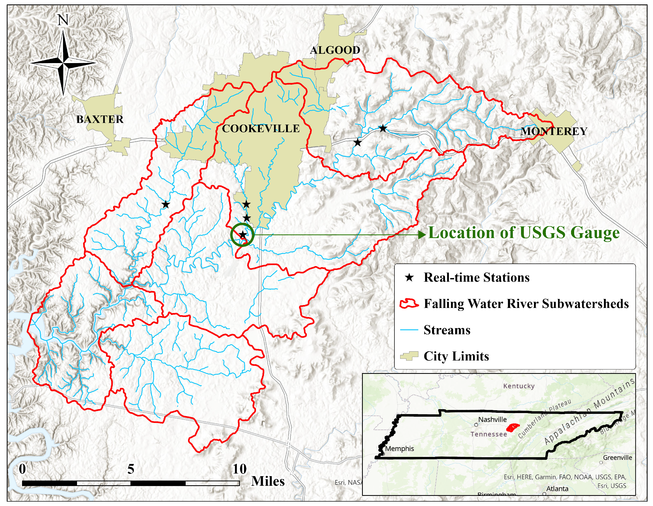
2.1. Case Study

Falling Water River (FWR) watershed was used as the study area for implementing the low-cost real-time water level monitoring system. It is located in middle Tennessee, covering parts of White, Dekalb, and Putnam Counties. At a Hydrologic Unit Code (HUC) level 10, it is a subwatershed of the Caney Fork watershed, which eventually drains into the Cumberland River. FWR watershed (HUC 0513010807), as seen in Figure 1, has an estimated 202 sq. mi., and is drained by the Falling Water River, which originates just west of Monterrey at the edge of Cumberland Plateau and traverses the Eastern Highland Rim before moving towards the Caney Fork River. Based on the National Land Cover Dataset (2011) [11], the land cover of the FWR watershed is 20% developed, 41% forested, and 36% agricultural cover. Most of the developed area is concentrated around Cookeville and Algood areas in the northern part of the watershed, and the headwaters of the tributaries to Falling Water River. At the time of writing this paper, only one USGS gage was available to monitor water level and streamflow along the mainstem of Falling Water River. In recent years, the region has seen significant flooding such as, the flooding in Dry Valley and Cummins Falls State Park [12] in a neighboring watershed. Hence, low-cost real-time water level monitoring solutions such as the system presented in this manuscript is beneficial for flood warning and management.

2.2. Methodology

The low-cost real-time water level monitoring network for the Falling Water River watershed was developed in phases. During the first phase, a working prototype of the water level sensor was developed, and tested in the laboratory for regular and correct distance measurements. The workflow of how the reading was measured and transmitted over the air to an online repository for a data visualization was developed. During the second phase, the prototype sensors were field tested. In the third phase, these field-tested sensors were deployed within the Falling Water River watershed. Finally, the data transmitted by the sensors were collected, stored, and visualized on a user-friendly web-based dashboard.

2.2.1. Assembly of Low-Cost Real-Time Water Level Sensor Prototype

A prototype of the low-cost real-time water level sensor (referred to as TNTech sensor or gage from now on) was developed. It was important for the sensor to have the following physical characteristics: easy-to-build, weather resistant, insect-proof, light-weight, easy to install, and not easily visible. It was also important for the sensor to have the following technical capabilities: internet enabled, low-power consumption, auxillary power, computationally efficient, easily programmable, over-the-air updates, etc. The components of the water level sensor can be categorized into four groups that include: micro-controller, circuit board, ultrasonic level sensor, power supply, and hardware peripherals.

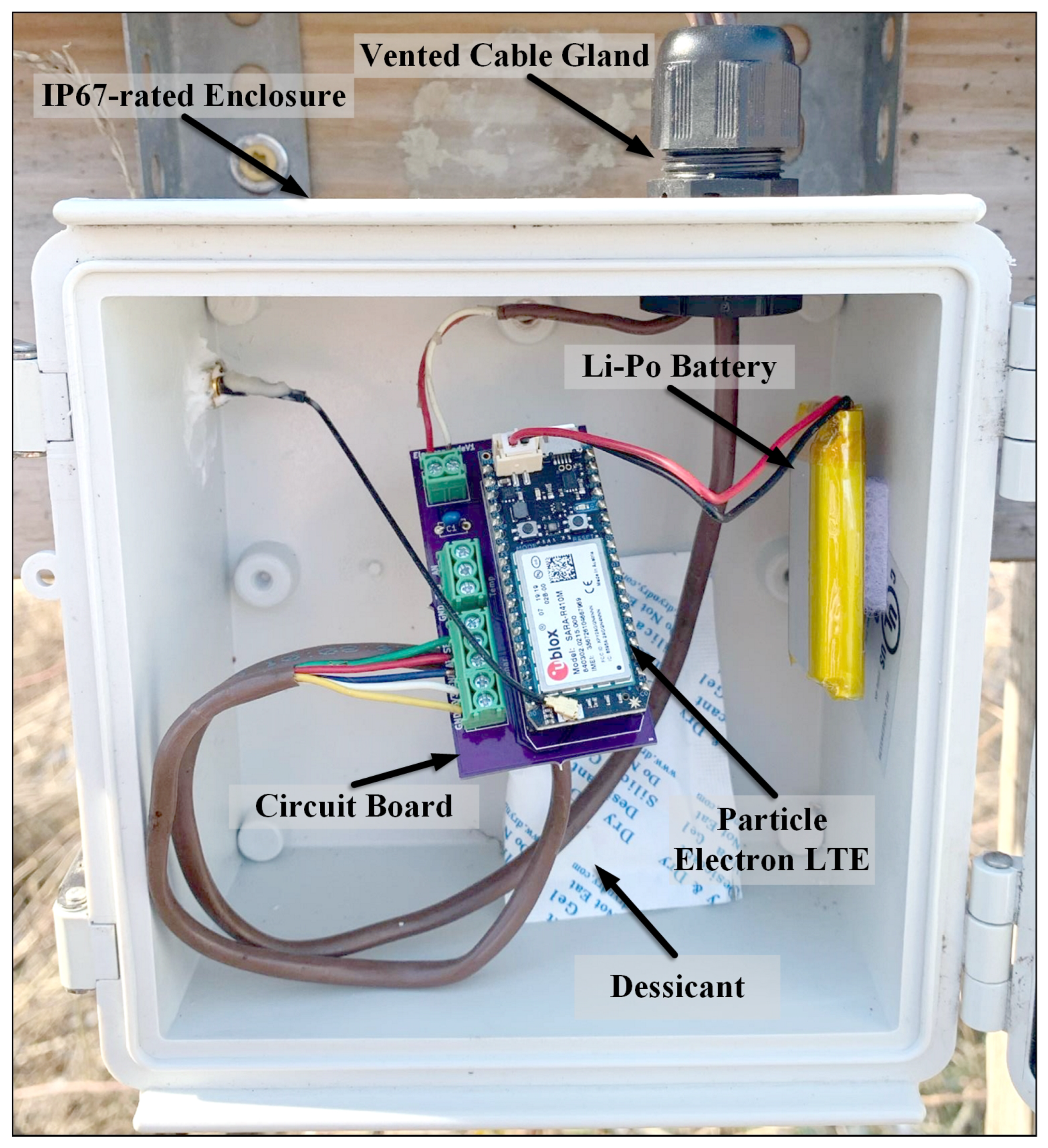
• Micro-controller: Based on these criteria, a sensor prototype was developed that included a Particle Electron LTE micro-controller platform. It is the main component of the sensor. The Particle Electron micro-controller platform follows an open-source design. It includes a STM32F205RGT6 ARM Cortex-M3 micro-controller which operates at a rate of 120 MHz. It can be updated by utilizing OTA updates. The Electron stores variables to carry a regular operation by using 128 KB of RAM and 1 MB of Flash ROM. This micro-controller is built using a MAX17043 battery monitor, which can measure the energy spent by the IoT node. The Particle Electron LTE supports LTE Cat M1 using a cellular module called U-blox SARA-R410M [13], and it enables an IP connection. A cellular antenna is enclosed for the micro-controller to establish a link to a nearby cellular tower [14]. This micro-controller acts as the central processing unit of the sensor. It is programmable to communicate with other electronic devices that are connected to it, and send and receive data from them. It is powered by a 3.7 V 1800 mAH Lithium Ion Polymer (Li-Po) battery and also connected to a 6 V 3.5 W Solar Panel that serves as an auxilliary power supply to recharge the battery;
• Circuit Board: The micro-controller is plugged into a custom-built circuit board as seen in Figure 2. This acts as the central location, to which all the electronics and electrical components are connected. The next crucial component is the ultrasonic water level sensor (see the next item);
• Ultrasonic level sensor: The ultrasonic level sensor used for the prototype is a MaxBotix XL-MaxSonar-WRMA1 sensor [15]. It is a IP-67 rated sensor that emits acoustic waves at 42 kHz and receives the return signal. Using the time elapsed and the speed of sound, calculates the distance traveled by the waves. To measure the water level, the ultrasonic level sensor is placed vertically facing the surface of the water in the waterbody. There may be other strategies to measure water depth, such as affordable pressure transducers. In this study, an ultrasonic sensor was used because it is a non-contact measurement strategy and at any point in the measurement, the equipment would not interact with the fast moving waters or floating debris, hence it can function reliably during high flow conditions. The choice of this particular ultrasonic sensor was based on previous studies conducted by Refs. [8,9,10];
• Power Supply: The main power supply is a 3.7 V 2000 mAh Li-Po battery [16], and the auxilliary power source is a 6 V 3.5 W Solar panel manufactured by Voltaic Systems [17];
• Hardware Peripherals: All the components of the water sensor are placed within a IP67 rated plastic box (approximately 6 inch × 6 inch × 3.5 inch) manufactured by Bud Industries [18]. The wires coming out of the box and connecting the solar panel and the ultrasonic sensors go through a vented cable gland [19], as shown in Figure 2.

The prototype is programmed in such a way that it comes online at regular intervals (e.g., every 15 min), connects to the Particle Cloud [20], and transfers the data (water level in inches and battery voltage) to the cloud, where it is available for data capture and storage in a repository (see Section 2.2.4).

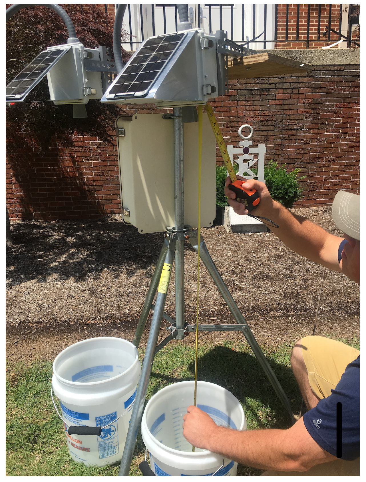
2.2.2. Field Testing of the Sensor Prototype

After the field prototype was developed, it was tested in the laboratory to ensure that the micro-controller comes online and connects to the Particle Cloud, and publishes the accurate data without fail. Following the laboratory testing, the sensor was placed outdoors on a stationary stand, with a bucket of water on the ground directly underneath it, as shown in Figure 3. The observed distance was 48.5 inches and the sensor measured within 5% relative error, which is sufficient for water level monitoring.

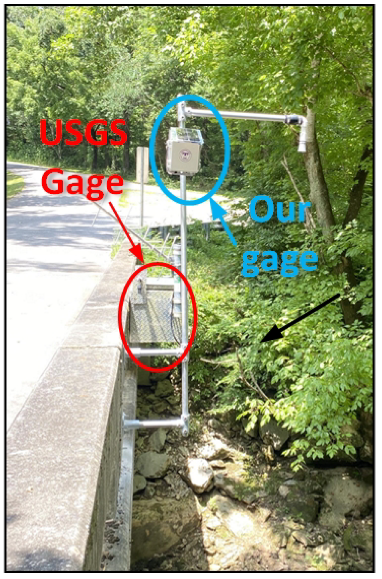
2.2.3. Sensor Deployment and Data Collection

Following the successful field testing of the prototype, six sensors were built, deployed at six locations within the Falling Water River Watershed, as shown by the “★” symbols in Figure 1. The accuracy of the TNTech gage will be estimated by comparing the water levels measured by the TNTech gage that was installed next to the USGS gage at Randolph Mill Rd (USGS Station No. 3423000) [21], as seen in Figure 4. Both the gages are installed on the Randolph Mill Rd bridge. From Figure 4, it is determined that the type of USGS gage is a radar gage.

For more details on the comparative analysis, see Section 2.2.5. It should be noted that the TNTech gages are non-contact devices and measure water surface elevations and also distance from the sensor to the water surface. Equation (1) explains how the water surface elevation (WSE) is converted to the water depth:

$$\mathrm{Water}\mathrm{Depth}=\mathrm{Water}\mathrm{Surface}{\mathrm{Elevation}}_{\mathrm{TNTech}\mathrm{Sensor}}-\mathrm{Invert}\mathrm{Elevation}$$

(1)

The invert elevation can be determined by manually measuring it at site or it can be estimated by using the water depth data from USGS. It should be noted that the accuracy of the TNTech gage is not only dependent on the ultrasonic sensor, but also on the invert elevation measured or estimated at site. In the current study, the invert elevation was estimated using the USGS water depth at known time and by subtracting it from the measured WSE by the TNTech gage to generate “apparent” water depths.

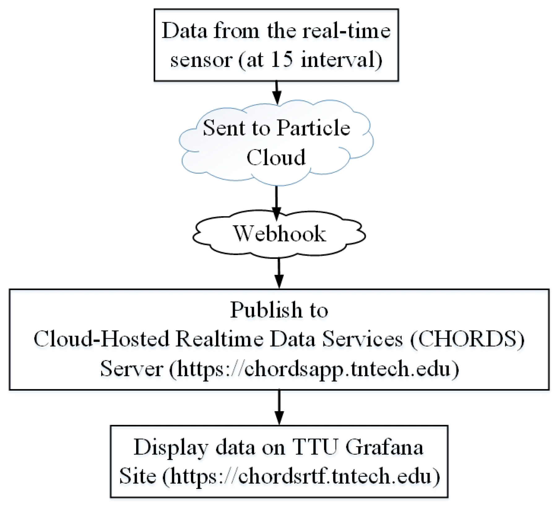
2.2.4. Data Storage and Visualization

The data from the device is not stored on board but transferred to a web-based database for storage and visualization. The web-based database portal is built using a software application called Cloud-Hosted Real-time Data Services (CHORDS), which was developed by scientists and researchers as a part of National Science Foundation’s EarthCube Initiative [22]. A CHORDS portal was launched as a preconfigured instance on Tennessee Tech University’s (TNTech’s) infrastructure, who deployed it with minimal setup overhead. Each TNTech’s CHORDS user would own and manage their own CHORDS instance and interface it with their data streams. A preconfigured web server on the instance hosts a user interface, which is used to define data streams that will be ingested by the instance. The CHORDS portal also has an interactive data visualization application called Grafana, available at Ref. [23], which serves as a front-end application for visualizing the data collected by the sensors. The workflow of data capture and storage is shown in Figure 5, and also explained at the end of Section 2.2.1.

2.2.5. Comparative Analysis

The performance of the low-cost real-time water level sensors developed in this study was tested by comparing its measurements with the USGS gage measurement. The comparison was performed at two levels: (i) event-based comparison and (ii) long-term comparison. For event-based comparison, few flow events from the period of record will be identified, and the datasets from the two gages will be compared using the following statistical metrics: Coefficient of Determination (R²), Nash–Suttcliffe Efficiency (NSE), Percent Bias (PBIAS), Mean Squared Error (MSE), Mean Absolute Error (MAE), and Root Mean Squared Error (RMSE). The performance evaluation criteria for R², NSE, and PBIAS metrics are presented in

Table 1. Statistical comparison metrics and evaluation criteria.

Measure	Performance Evaluation Criteria
	Very Good	Good	Satisfactory	Not Satisfactory
Coefficient of Determination (R2)	$R^2>0.85$	$0.75<R^2\le 0.85$	$0.60<R^2\le 0.75$	$R^2\le 0.60$
Nash–Suttcliffe Efficiency (NSE)	$NSE$ > 0.80	$0.70<NSE\le 0.80$	$0.50<NSE\le 0.70$	$NSE\le 0.50$
PBIAS (%)	$PBIAS<\pm 5$	$\pm 5<PBIAS\le \pm 10$	$\pm 10<PBIAS\le \pm 15$	$PBIAS\ge \pm 15$
MSE	Optimal Value is 0.0
MAE
RMSE

, adapted from Ref. [24]. A review of the literature did not yield any published evaluation criteria for MSE, MAE, and RMSE, but optimal values for these metrics were reported to be 0.0 [24].

The long-term comparison was performed using two statistical analyses, namely Wilcoxon Signed-Rank Test [25] and Loess Seasonal Decomposition [26]. The Wilcoxon Signed-Rank Test was used to evaluate the differences in the datasets.The Loess Seasonal Decomposition allows for a time series to be separated into its trend, seasonal variation, and residual. This analysis allowed us to not only compare the trends seen in the data, but also determine if the long term variations in the data (caused by seasonality) match up between the gages.

3. Results and Discussion

This section presents the results of the comparative analysis of observed water levels from the USGS gage with the water level data measured by our low-cost sensor. The time period of analysis was 2020 to 2022, and it was performed in two levels: (i) event-based comparison and (ii) long-term comparison. For the event-based comparison, nine high-flow events over the period of record were identified, as listed in

Table 2. Selected storm events for analysis.

Event Number	Time Period	Storm Depth (in.)
Event 1	12/9/2021 to 12/14/2021	1.26
Event 2	12/28/2021 to 01/06/2022	3.67
Event 3	01/7/2022 to 01/13/2022	1.54
Event 4	01/14/2022 to 01/19/2022	3.45
Event 5	02/01/2022 to 02/08/2022	1.75
Event 6	02/19/2022 to 03/05/2022	5.7
Event 7	04/09/2022 to 04/21/2022	4.7
Event 8	07/16/2022 to 07/25/2022	2.03
Event 9	09/01/2022 to 09/07/2022	3.18

.

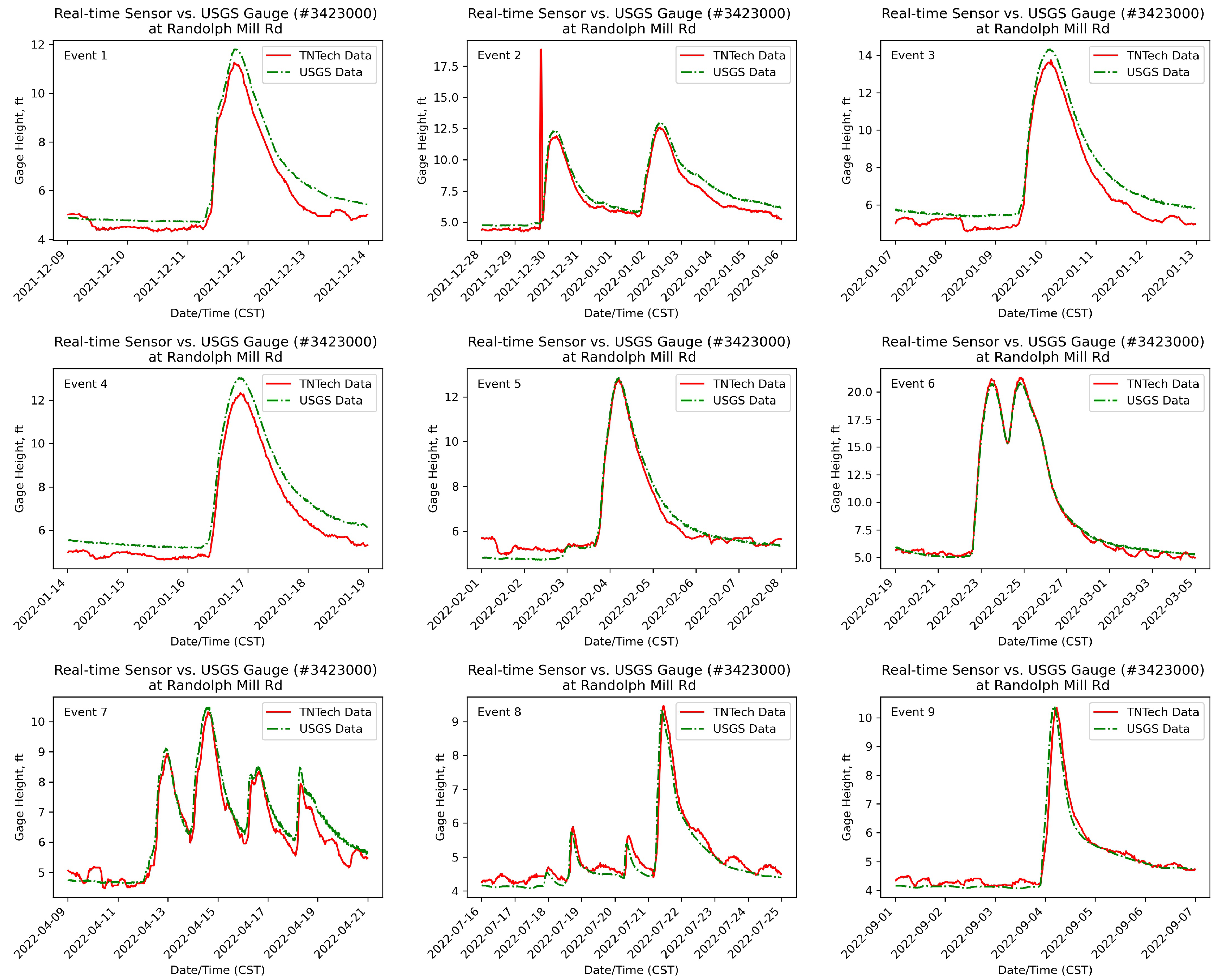
3.1. Event-Based Comparison

The results of the event-based comparison is presented in

Table 3. Event-based comparison and performance.

Event	R2		NSE		PBIAS		MSE (ft2)	MAE (ft)	RMSE (ft)
	Value	Performance	Value	Performance	Value	Performance
Event 1	0.98	Very Good	0.94	Very Good	7.01	Good	0.26	0.45	0.51
Event 2	0.87	Very Good	0.81	Very Good	6.80	Good	1.06	0.61	1.03
Event 3	0.99	Very Good	0.92	Very Good	9.58	Good	0.57	0.71	0.75
Event 4	0.99	Very Good	0.91	Very Good	9.53	Good	0.5	0.68	0.71
Event 5	0.98	Very Good	0.97	Very Good	−0.60	Very Good	0.12	0.28	0.35
Event 6	1.00	Very Good	1.00	Very Good	0.31	Very Good	0.1	0.26	0.31
Event 7	0.96	Very Good	0.94	Very Good	3.51	Very Good	0.15	0.31	0.39
Event 8	0.97	Very Good	0.94	Very Good	−3.56	Very Good	0.07	0.21	0.26
Event 9	0.97	Very Good	0.96	Very Good	−2.25	Very Good	0.07	0.17	0.27

. It is clear from these metrics that our low-cost sensor performed very well in measuring the water depths when compared to the USGS gage for almost all the nine events. The R² value and NSE values were considered “Very Good” for all events, while PBIAS values were considered “Very Good” for five out of nine events. The remaining four events were considered “Good”, as they had slightly higher values of MSE, MAE, and RMSE. These results are confirmed by the hydrograph comparison of all the nine events presented in Figure 6.

It can be observed that during Events 1 through to 4, the water level measured from the low-cost sensor was underestimated, causing the MAE, MSE, and RMSE values to be larger than the remaining events, and resulting in “Good” for R², NSE, and PBIAS values. Overall, at individual event scale, these comparisons clearly indicate that the water levels measured by the low-cost sensor and the USGS gage are very close. In the current study’s context, this error range for water level monitoring is considered acceptable. However, if the water level readings from these low-cost sensors are applied to estimate discharge calculations, these errors can potentially significantly influence discharge estimations. Additional testing of the accuracy of low-cost sensors for discharge calculations may be warranted under those situations.

3.2. Long-Term Comparison

The two datasets were also examined over a longer time period (2020 to 2022) to verify how well the low-cost sensor data compares to the USGS gage data. For this task, two statistical analyses, namely Wilcoxon Signed-Rank Test [25] and Loess Seasonal Decomposition [26], were used.

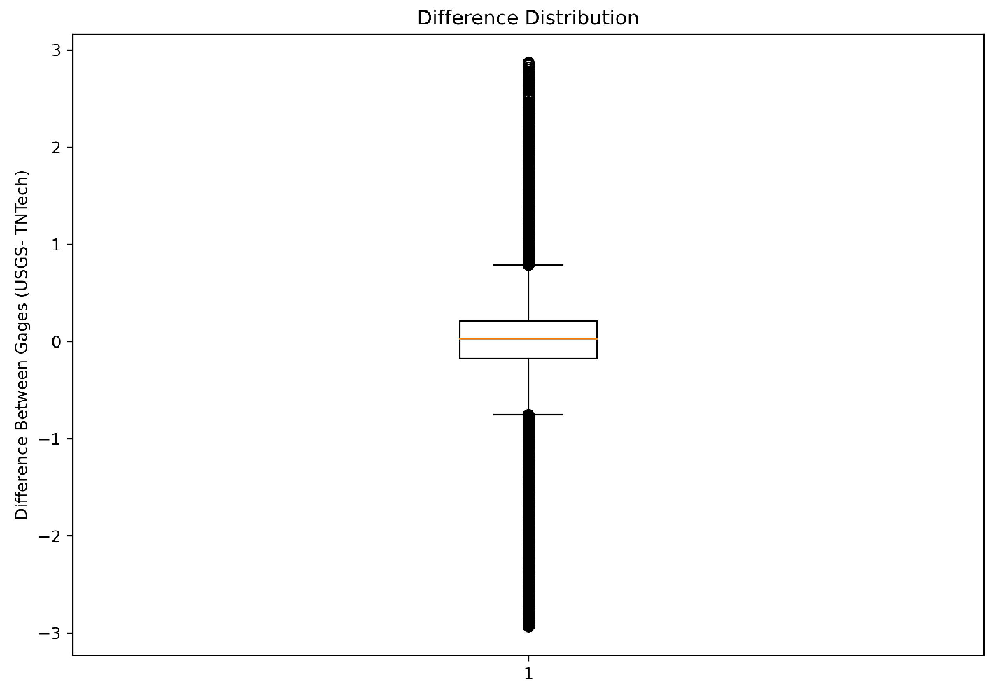
3.2.1. Wilcoxon Signed-Rank Test

The Wilcoxon Signed-Rank test is a nonparametric statistical comparison test. The null hypothesis of the test states that the median difference between the two datasets is 0 [27]. When looking at the complete datasets, it was found that the data is significantly different at the 0.05 alpha level. In order to evaluate where the differences lie, a box plot of the difference of the USGS data and the TNTech data is shown in Figure 7.

It can be seen from this figure that the median is around zero, with the majority of the points falling above one. This shows that the USGS gage tends to measure higher water levels compared to the TNTech gage over the course of the sampling period. However, when the analysis is focused on individual events, the Wilcoxon comes back as non-significant. The same effect can be seen when the datasets are averaged by longer periods (hours, days, etc.) and the test results come back as non-significant. Therefore, it appears that when the datasets were compared in their totality, the number of observations could have led to a significant difference.

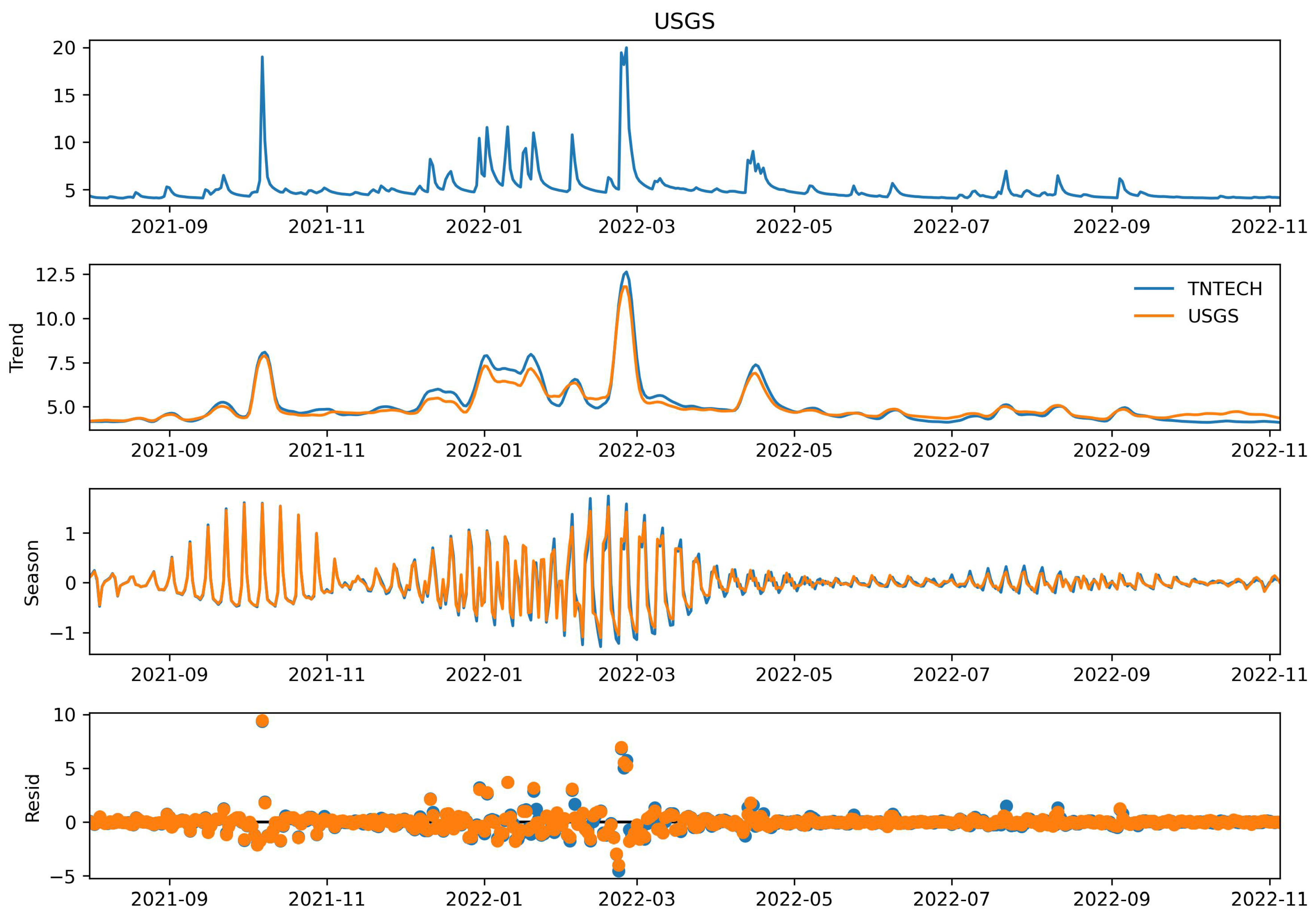
3.2.2. Loess Seasonal Decomposition

The Loess Seasonal Decomposition splits each time series into its trend, seasonality, and residuals components. This analysis was developed by Ref. [26] to create a straightforward method of breaking down time series into their components and smoothing. For this analysis, each time series (USGS, TNTech) was split into its components and compared to the corresponding component of the other dataset. These graphs can be seen in Figure 8. From this figure, it can be observed that the trend lines of the TNTech dataset are similar to the USGS data, constantly being higher than the TNTech gage.

As can be seen in the residual plot (bottom panel in Figure 8, despite some deviations in water level measurements (such as during October 2021, March 2022, and April 2022), the TNTech gage followed the same trends in all components (see the second and third panels in Figure 8). In essence, the measurement from the TNTech gage may be off a little bit, but this difference was consistent throughout the time period of the analysis. This difference can be due to the usage of “apparent” water depth calculated for the TNTech gage. The comparison could be better if an observed water depth was used to convert the WSE values of the TNTech gage to generate water depths (see Section 2.2.3 for more details on water depth estimation). It can be seen that each of the components of the time series appear to match well. This indicates that the scale of changes recorded by the TNTech sensor match those of the USGS gage.

A percent change comparison of each of the two datasets was also performed, which measures the percentage of difference in water depths between the successive timesteps of the corresponding datasets. Figure 9 presents the percent differences of these two datasets plotted against each other.

A perfect correlation between these two datasets would represent that the two datasets are measuring the same change in percent difference of water depths in all the timesteps. It would not indicate the accuracy of one dataset in predicting the other, but rather the gages are reading the same relative changes. It can be observed from Figure 9 that correlation does have a slope closer to 1, which would mean that the two datasets have comparable changes in their corresponding measurements. This is important because the TNTech gage values can be skewed based on multiple reasons (e.g., incorrect or inaccurate invert elevation, inaccurate GPS elevation, etc.), but this comparison shows that the TNTech gage experiences the same changes as the USGS gage. Therefore, the TNTech gage readings can be considered accurate from this relative comparison.

4. Summary

The comparative analysis of the TNTech gage with respect to the USGS gage, presented in Section 3, shows very good agreement. The event-based comparison (see Section 3.1) was performed for nine storm events, whose storm depths range from 1.25 inches and 5.7 inches and durations vary between 5 h and 17 days. Based on the metrics by Ref. [24], the TNTech sensor data showed a “Very Good” comparison to USGS data in terms of R², NSE, and PBIAS (except for Events 1 through to 4). Hence, it is determined that TNTech water level data was comparable with the USGS water level data on the event scale. It should be noted that the water level readings from these low-cost sensors may not be applied to estimate discharge calculations without additional accuracy tests, as these errors can potentially significantly influence discharge estimations.

To account for a longer term comparison, an additional comparison was also presented using Wilcoxon Signed-Rank Test and Loess Seasonal Decomposition analysis, presented in Section 3.2. The first comparison showed that the TNTech gage slightly underestimated the water depths over the sampling period, but when evaluated at the event-scale, this underestimation was non-significant. This was confirmed when the timestep was averaged by longer periods (hours and days). Similarly, the Loess Seasonal Decomposition Analysis (see Section 3.2.2) showed good agreement between the two datasets. A comparison of the percent difference in water depth in successive timesteps of the two datasets showed a good correlation gage readings, and hence TNTech gage readings can be considered accurate from this relative comparison.

The Maxbotix MB 7092 sensors that were purchased in this project came with a “full horn” housing that protects the sensor (please see Ref. [15]). The TNTech gage at the Randolph Mill Rd, which collected data during the period of 2020 to 2022, did not have any issues with ingress of foreign objects. However, the TNTech gage was offline during the March 2021 flood event, and hence there is a 4-month period during 2021 in which the data was not measured. During the March 2021 flood event, the USGS gage was also flooded and was offline [28] around the same time. It was later replaced by USGS with a newer gage.

While the current study shows the feasibility of low-cost real-time water level sensors and their performance comparison to a state-of-the-art USGS gage, more work needs to be done in the future. These tasks include: re-doing the comparison for an even longer time period (e.g., 5-year, 10-year etc.), placing sensors at other USGS locations with different baseflow conditions and evaluating the performance, testing the impact of the initial invert elevations on the water level data, extracting water surface elevations and flood inundation extents using this data, and checking the feasibility of using these low-cost gages for water level forecarsting. Overall, this study clearly demonstrates the successful implementation of a low-cost real-time solution for water level monitoring and paves the way for future applications in flood forecasting.

References

1. Smith, A.B. U.S. Billion-Dollar Weather and Climate Disasters, 1980-Present; NCEI Accession 0209268; National Oceanic and Atmospheric Administration, National Centers for Environmental Information: Biloxi, MI, USA, 2020. [CrossRef]
2. Špitalar, M.; Gourley, J.J.; Lutoff, C.; Kirstetter, P.E.; Brilly, M.; Carr, N. Analysis of flash flood parameters and human impacts in the US from 2006 to 2012. J. Hydrol. 2014, 519, 863–870. [Google Scholar] [CrossRef]
3. USGS. USGS Streamgaging Network. 2022. Available online: https://www.usgs.gov/mission-areas/water-resources/science/usgs-streamgaging-network (accessed on 26 December 2022).
4. Normand, A.E. U.S. Geological Survey (USGS) Streamgaging Network: Overview and Issues for Congress. 2020. Available online: https://crsreports.congress.gov/product/pdf/R/R45695 (accessed on 26 December 2022).
5. Castillo-Effer, M.; Quintela, D.H.; Moreno, W.; Jordan, R.; Westhoff, W. Wireless Sensor Networks for Flash-Flood Alerting. In Proceedings of the Fifth IEEE International Caracas Conference on Devices, Circuits and Systems, Punta Cana, Dominican Republic, 3–5 November 2004; Volume 1, pp. 142–146. [Google Scholar]
6. Zhang, Z.; Glaser, S.D.; Bales, R.C.; Conklin, M.; Rice, R.; Marks, D.G. Technical report: The design and evaluation of a basin-scale wireless sensor network for mountain hydrology. Water Resour. Res. 2017, 53, 4487–4498. [Google Scholar] [CrossRef]
7. Zhang, D.; Heery, B.; O’Neil, M.; Little, S.; O’Connor, N.E.; Regan, F. A low-cost smart sensor network for catchment monitoring. Sensors 2019, 19, 2278. [Google Scholar] [CrossRef] [PubMed]
8. Kerkez, B.; Gruden, C.; Lewis, M.; Montestruque, L.; Quigley, M.; Wong, B.; Bedig, A.; Kertesz, R.; Braun, T.; Cadwalader, O.; et al. Smarter stormwater systems. Environ. Sci. Technol. 2016, 50, 7267–7273. [Google Scholar] [CrossRef] [PubMed]
9. Wong, B.P.; Kerkez, B. Real-time environmental sensor data: An application to water quality using web services. Environ. Model. Softw. 2016, 84, 505–517. [Google Scholar] [CrossRef]
10. Mullapudi, A.; Bartos, M.; Wong, B.; Kerkez, B. Shaping Streamflow Using a Real-Time Stormwater Control Network. Sensors 2018, 18, 2259. [Google Scholar] [CrossRef] [PubMed]
11. Homer, C.; Dewitz, J.; Yang, L.; Jin, S.; Danielson, P.; Xian, G.; Coulston, J.; Herold, N.; Wickham, J.; Megown, K. Completion of the 2011 National Land Cover Database for the conterminous United States–representing a decade of land cover change information. Photogramm. Eng. Remote Sens. 2015, 81, 345–354. [Google Scholar]
12. After Flooding Deaths at Cummins Falls, NWS Ramps up Communication Efforts. 2022. Available online: https://www.tennessean.com/story/news/2017/08/17/after-flooding-deaths-cummins-falls-nws-ramps-up-communication-efforts/575550001/ (accessed on 1 December 2022).
13. u blox. SARA-R4 Series LTE-M/NB-IoT/EGPRS Modules with Secure Cloud. 2023. Available online: https://www.u-blox.com/en/product/sara-r4-series (accessed on 26 December 2022).
14. Trilles, S.; González-Pérez, A.; Zaragozí, B.; Huerta, J. Data on records of environmental phenomena using low-cost sensors in vineyard smallholdings. Data Brief 2020, 33, 106524. [Google Scholar] [CrossRef] [PubMed]
15. MaxBotix. MB7092 XL-MaxSonar-WRMA1. 2023. Available online: https://maxbotix.com/products/mb7092 (accessed on 26 December 2022).
16. Adafruit. Lithium Ion Battery-3.7 V 2000 mAh. 2023. Available online: https://www.adafruit.com/product/2011 (accessed on 26 December 2022).
17. Systems, V. 3.5 Watt 6 Volt Solar Panel. 2023. Available online: https://voltaicsystems.com/3-5-watt-panel/ (accessed on 26 December 2022).
18. Industries, B. PTQ-11046. 2023. Available online: https://www.digikey.com/en/products/detail/bud-industries/PTQ-11046/5291540 (accessed on 26 December 2022).
19. Conta-Clip, I. 97741.1 Cablegland. 2023. Available online: https://www.digikey.com/en/products/detail/conta-clip-inc/97741-1/10205549 (accessed on 26 December 2022).
20. Particle. Device Cloud: A Secure, Scalable, and Reliable Cloud Platform to Manage Your Fleet of IoT Devices. 2022. Available online: https://www.particle.io/device-cloud/ (accessed on 2 April 2022).
21. United States Geological Survey. USGS 03423000 Falling Water River near Cookeville, TN. 2022. Available online: https://waterdata.usgs.gov/nwis/inventory?site_no=03423000 (accessed on 26 December 2022).
22. Kerkez, B.; Daniels, M.; Graves, S.; Chandrasekar, V.; Keiser, K.; Martin, C.; Dye, M.; Maskey, M.; Vernon, F. Cloud Hosted Real-time Data Services for the Geosciences (CHORDS). Geosci. Data J. 2016, 3, 4–8. [Google Scholar] [CrossRef]
23. Tennessee Technological University. Home-Grafana. 2022. Available online: https://chordsrtf.tntech.edu/ (accessed on 2 April 2022).
24. Moriasi, D.N.; Gitau, M.W.; Pai, N.; Daggupati, P. Hydrologic and water quality models: Performance measures and evaluation criteria. Trans. ASABE 2015, 58, 1763–1785. [Google Scholar]
25. Rosner, B.; Glynn, R.J.; Lee, M.L.T. The Wilcoxon signed rank test for paired comparisons of clustered data. Biometrics 2006, 62, 185–192. [Google Scholar] [CrossRef] [PubMed]
26. Cleveland, R.B.; Cleveland, W.S.; McRae, J.E.; Terpenning, I. STL: A Seasonal-Trend Decomposition Procedure Based on Loess (with Discussion). J. Off. Stat. 1990, 6, 3–73. [Google Scholar]
27. Wilcoxon, F. Individual Comparisons by Ranking Methods. Biom. Bull. 1945, 1, 80–83. [Google Scholar] [CrossRef]
28. USGS. Falling Water River near Cookeville, TN. 2023. Available online: https://waterdata.usgs.gov/monitoring-location/03423000/#parameterCode=00065&startDT=2021-03-26&endDT=2021-03-30, (accessed on 26 December 2022).
Figure 1. Falling Water River watershed.
Geosciences 13 00065 g001
Figure 2. Components of the water level sensor.
Geosciences 13 00065 g002
Figure 3. Field test of the sensor prototype.
Geosciences 13 00065 g003
Figure 4. Location of our TNTech Gage in relation to USGS Gage (#3423000).
Geosciences 13 00065 g004
Figure 5. Components of the water level sensor.
Geosciences 13 00065 g005
Figure 6. Hydrograph comparison for all nine events.
Geosciences 13 00065 g006
Figure 7. Box plot comparison of the differences between TNTech and USGS water levels.
Geosciences 13 00065 g007
Figure 8. Comparison of the time series components using Loess Seasonal Decomposition.
Geosciences 13 00065 g008
Figure 9. Percent change in the depth comparison between the gages.
Geosciences 13 00065 g009