Article

Seasonal Dynamics of Gaseous CO2 Concentrations in a Karst Cave Correspond with Aqueous Concentrations in a Stagnant Water Column

1
Institute for Modelling Hydraulic and Environmental Systems, University of Stuttgart, 70569 Stuttgart, Germany
2
GFZ German Research Centre for Geosciences, 14473 Potsdam, Germany
*
Author to whom correspondence should be addressed.
Geosciences 2023, 13(2), 51; https://doi.org/10.3390/geosciences13020051
Submission received: 6 December 2022 / Revised: 27 January 2023 / Accepted: 31 January 2023 / Published: 6 February 2023

Abstract

:
Dissolved CO2 in karst water is the key driving force of karstification. Replenishment of CO2 concentrations in karst water occurs by meteoric water that percolates through the vadose zone, where CO2 produced from microbial activity is dissolved. CO2 can thus be transported with the percolating water or in the gas phase due to ventilation in karst systems. We measured seasonally fluctuating CO2 concentrations in the air of a karst cave and their influence on aqueous CO2 concentrations in different depths of a stagnant water column. The observed data were compared to numerical simulations. The data give evidence that density-driven enhanced dissolution of gaseous CO2 at the karst water table is the driving force for a fast increase of aqueous CO2 during periods of high gaseous concentrations in the cave, whereas during periods of lower gaseous concentrations, the decline of aqueous CO2 is limited to shallow water depths in the order of 1 m. This is significant because density-driven CO2 dissolution has not been previously considered relevant for karst hydrology in the literature. Attempts at reproducing the measured aqueous CO2 concentrations with numerical modeling revealed challenges related to computational demands, discretization, and the high sensitivity of the processes to tiny density gradients.

Graphical Abstract

1. Introduction

Karstic rock covers on the order of 10% of the continental surface and is found in many parts of the world (e.g., [1,2,3]). Karst systems can be viewed as snapshots of native rocks resulting from of a complex interplay of predominantly hydraulic and chemical processes in mainly carbonate rocks, and many karst systems keep evolving strongly today. CO2 is a key player in rock corrosion (i.e., karstification). It forms carbonic acid in the presence of water, which can eventually dissolve limestone (CaCO3) or dolomite (CaMg[CO3]2). It is common ground in textbooks that the main source of the CO2 in epigenetic karst systems is produced from microbiological processes and root respiration in the vadose zone [1,3,4,5,6,7]. Much of the dissolving power of CO2-enriched water is consumed in the topmost layers of a karst system and leads to denudation and an extensive near-surface erosion of a karstic landscape. However, cavities in karst systems can obviously also grow deep inside of rocks, and there are different explanations discussed in the literature. Mixing corrosion describes the phenomenon that the mixing of two (or more) water streams (e.g., in a joint deep in the rock), always results in a calcite-aggressive mixed water [8]. Another explanation for corrosion deep in the rock is found in non-linear dissolution kinetics [9,10,11,12]. It says that flowing water retains some residual dissolving power until deep inside the rock. We note that both phenomena—mixing corrosion and non-linear dissolution kinetics—require hydraulic gradients and, accordingly, an advective flow or percolation of water to replenish carbonate-dissolution potential deep inside the rock. In addition to that, it was recently proposed that a pathway via the gas phase in the vadose zone can also contribute to replenishing carbonic acid even in stagnant water [13]. In such conditions, the process of replenishment with CO2 crucially relies on density-driven enhanced dissolution of CO2 (or convective mixing), which is a well known and very significant mechanism in long-term trapping of CO2 that is injected into deep geologic formations (e.g., [14,15]). The importance of gas-phase advection for CO2 dynamics in particular for deep karst systems was also highlighted by the work of [16], although the study did not address convective mixing in the water. The study of [13] demonstrated that density-driven enhanced dissolution of CO2 can contribute in karst systems up to an order of 10–100 g CO2 per month and square meter of karst water table at typical CO2 concentrations in cave air (e.g., at 2% CO2). This can be significant as it would allow carbonate dissolution and, thus, growth of cavities even during periods where water comes to rest in a cavity or a fracture. A potential relevance of this process for karstification and speleogenesis has not yet been discussed or quantified in the karst literature.
However, in the context of porous-media research and CO2 geological storage, many numerical studies and analyses of (in-)stability address convective mixing of CO2 in water or brine [17,18,19,20,21,22,23]. These authors conclude that Darcy-type porous-media models require very small discretization lengths to resolve onset time and fingering patterns correctly [19,24]. This implies that grid-converged results on large spatial reservoir scales are practically infeasible.
This study, however, puts the focus on water bodies in karst structures, where the Darcy equation is not valid, but rather the Navier–Stokes equations are required. Accordingly, this involves a significantly higher degree of complexity and results in even more computational effort. We keep this in mind when we later on discuss results of this study and compare experimental data with numerical simulations.
Ref. [13] employed an experimental laboratory setup in the form of a vertical column of water, which was initially in equilibrium with ambient CO2 concentrations, cooled down to 10 °C, and exposed to an average concentration of 2% CO2 in the head space at the water table. In different depths of the water column, the rise of the CO2 concentration was monitored during a period of two months and compared to numerical simulations with a Navier–Stokes model, where the density of water was dependent on the concentration of dissolved CO2. In good agreement between measurements and simulations, the dynamics of density-driven CO2 dissolution were quantified and their potential relevance for karst hydrology was substantiated. However, in order to improve the process understanding for karst settings, there are important challenges to be addressed. These include (i) describing the full interactions of the calco-carbonic system (i.e., a coupling of the compositional flow and transport processes with reaction kinetics of carbonate dissolution and corresponding changes in morphology (e.g., fracture aperture, porosity)), and (ii) a further improved knowledge on the CO2 concentration dynamics for more realistic karst conditions, which mainly involve strong seasonal fluctuations of CO2 concentration in the cave air and their correspondence with concentrations of dissolved CO2 at different depths below the karst water table.
This research addresses the second aspect and provides novel well-controlled measurement data generated in a karst cave. Two significant advances are accomplished in comparison to the previous study of [13]. First, we measured here continuously and in high temporal resolution the CO2 dynamics during a much longer period of time (i.e., 1 year and 4 months), during which the water was exposed to real cave-air conditions with naturally alternating periods of concentration gradients at the gas–water interface directing at times into the water body and at times out of it. Second, the data allow for distinguishing the characteristics of periods during which density-driven CO2 dissolution replenishes the water with CO2, and, on the other hand, periods during which gaseous CO2 concentrations are lower and degassing takes place at the gas–water interface. Importantly, it can be shown that CO2 entry rates into water are significantly higher during such inward-directed periods than release rates during outward-directed periods. Major aims of this study are the quantification of these dynamics under well-controlled conditions in an artificially created water body by monitoring the CO2 concentrations in the air and in different water depths as well as the interpretation of the measurements with support of meteorological data and numerical simulations. The dataset is published separately [25] and is available with detailed explanations for researchers who want to use it, for example, to reproduce it with their numerical models. As will be explained further on, our own attempts to reproduce the data with our available numerical simulation capabilities were not fully satisfactory, as the governing processes appear to be extremely sensitive to simplifying model assumptions.
The following section introduces the experimental setup and the numerical model that is used for the comparison between experiment and simulation results. After that, the results of both experimental observations and numerical simulations are presented, before the results are discussed and summarized in conclusions.

2. Materials and Methods

Based on the previous work in [13], the basic subject of investigation is a 6 m tall column of water in a cylindrical tube of about 0.25 m in diameter. In an experimental monitoring campaign, the primary focus is on the seasonal dynamics of CO2 concentrations in cave air and how they correspond with concentrations of dissolved CO2 in different depths of the water column. During the measurements, the column was open to the atmosphere at the top (i.e., at the water table and closed everywhere else).

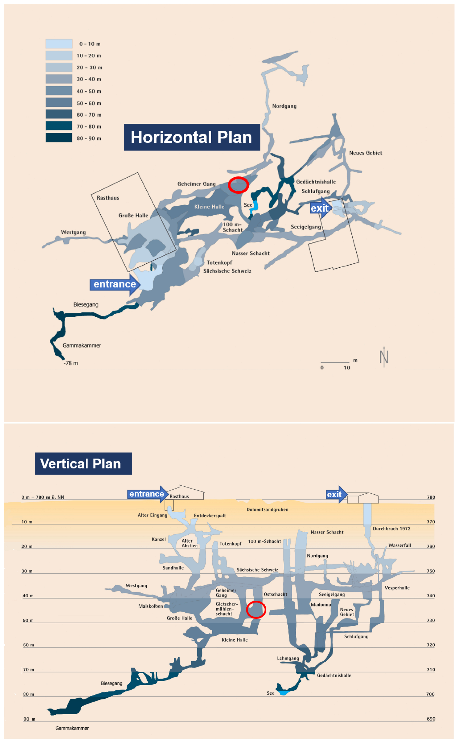
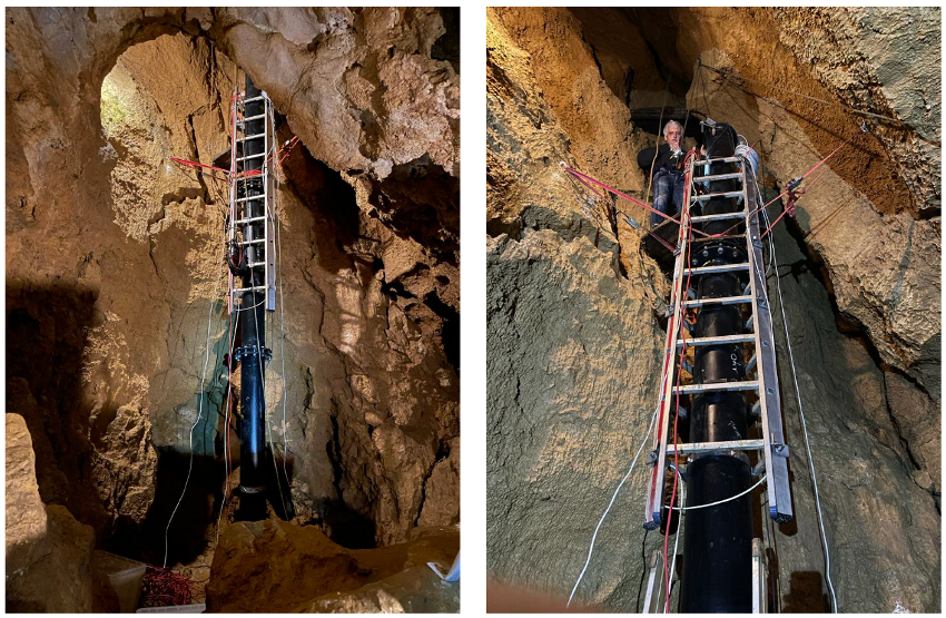
2.1. The Site of the Measurement Campaign

The experimental setup was installed at the bottom of a vertical side shaft in a 90 m deep cave, known as Laichinger Tiefenhöhle (48°28′42.9″ N 9°41′35.9″ E, 780 m a.s.l.), in the Swabian Jura/Southern Germany. The Swabian Jura is known for its multitude of karst caves in carbonate rocks, which are limestone formations. In the case of the Laichinger Tiefenhöhle, the rock also has contributions from dolomite. There are significantly elevated concentrations of CO2 in the cave air, which fluctuate strongly during the year. From our own (unpublished) preliminary sample measurements, it was known that CO2 concentrations in the cave air are in a range between 1% and 2% in the depth of the cave. The Laichinger Tiefenhöhle is a show cave and accessible for visitors. Thus, a connection to a power supply for the measurement equipment is easily possible at this depth. The experiment is located close to the deepest point of the visitor-accessible path at a depth of about 50 m below ground surface; see Figure 1.
Access to the cave is possible through doors in two buildings at the ground surface. Visitors can enter the cave except during the winter months; they descend into and ascend from the cave mostly along metal ladders anchored in the rock.
Today, the cave is no longer connected to the karst water table, which is several tens of meters below its deepest accessible point. The morphology of the cave was described recently by [26] (in the German language), including a large number of illustrations. Among many other formations, the author also notes spherical cavities that were supposedly developed in stagnant water, but the author does not discuss the origin of the CO2 or the dissolving power in detail. Larger wind speeds are not known in the cave; however, measurements are not available.
This region of the Swabian Jura is also known for the occurrence of so-called ‘Hungerbrunnen’, which are episodic karstic springs that pour water only after large precipitation events. This implies that parts of the karstic rocks in the Swabian Jura contain a kind of overflow system, which may give rise to the assumption that there are areas of episodic stagnant water in contact with the vadose zone. The general hydrogeology of the regional karstic system is explained in detail by [27] (in the German language). Based on their groundwater age determination, these authors postulate that some facies in the karst of this region have a high groundwater storage capacity and that observed quick reactions of karstic springs after precipitation events are explained by a piston flow effect, which is a pressure reaction in the sense that older, already stored groundwater is forced out of the system by successive inflows of new water. We will address a possible relation between precipitation events and CO2 concentration in cave air in the presentation of the results and in the discussion section.

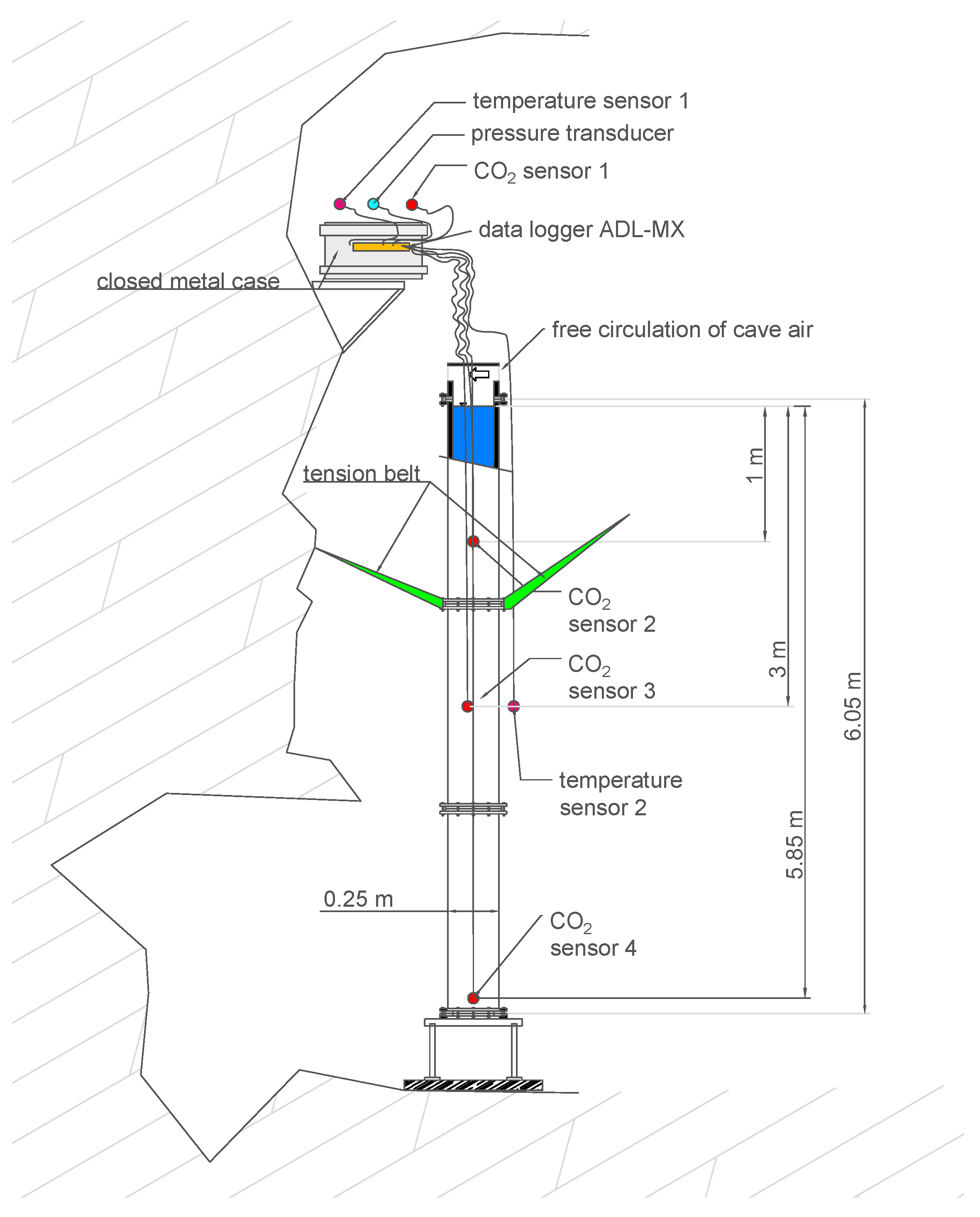
2.2. Monitoring CO2 Concentrations in Air and Water

A schematic of the experimental setup is given in Figure 2. The cylindrical tube was bolted to a metal frame at the bottom of a deep side shaft of the cave about 50 m below ground surface. The pipe was braced to the cave wall with three tension belts at a height of about 4 m. Ladders were attached to the column (see Figure 3) in order to allow for climbing up to the technical equipment, which was stowed in a closed metal case and placed on a small table that was anchored to the cave wall about 7 m from the bottom, above the top of the water column.
Vaisala GMP252 infrared gas sensors (factory-calibrated 0 − 20, 000e−6 [mol/mol], accuracy ± 1.5%) were used for monitoring the CO2 concentrations every minute both in the cave air and for the measurements in depths of 1 m, 3 m, and 5.85 m below the water table. The use of these sensors below the water table was tested under well-controlled laboratory conditions in our previous study [13]. For that purpose, a membrane covering was employed, which was water-proof and CO2 permeable. The PVC-based membrane had a thickness of 1.4 mm, which corresponds with a CO2 permeability of about 15 barrer [28] (1 barrer = 1 × 10 10 mL(SPT)/(s cm cmHg) = 7.5006 × 10 18 m3 s/kg). The direct CO2 measurements after membrane-based water–gas partitioning for long-term monitoring campaigns was applied and successfully proved in other studies (e.g., [29,30,31,32]). The response time of the Vaisala GMP252 sensors was tested with certified check gas at 0.1 MPa. Equilibrium was reached after about 1 h exposure time, which is considered fast enough to resolve concentration changes during a monitoring period of more than a year. The four sensors (one in the cave air, without membrane; three in the water body) were connected to a data-acquisition system (ADL-MX Advanced Datalogger, Meier-NT). They require 24 V power, supplied via a 10 m DC power cable. The water-proof sealing of the membrane and the cable-to-sensor connection was achieved with a self-vulcanization tape (3 M).
A calibration of the sensors according to the manufacturer’s (Vaisala) specifications occurred at conditions of 1013 hPa and 25 °C. Thus, the concentration signals required correction for deviations in temperature and pressure. Operating the sensors under hydrostatic conditions in up to 6 m water depth is a significant deviation from the designated use of these sensors at atmospheric conditions. Therefore, after consultation with the manufacturer, the following equation was applied for the corrections:
c c = c m · 1013   hPa · ( T / ( 298 [ K ] p ) )
where c c denotes the corrected and c m the measured CO2 concentration in parts per million (i.e., × 10 6 [mol/mol]) or percent; T is the temperature in Kelvin, and p the pressure in hPa during the measurement. Pressure correction includes the hydrostatic pressure for the sensors in the water body as well as the fluctuations of atmospheric pressures for all sensors; for measured pressure data, we refer to Appendix A. A pressure transducer continuously monitored the fluctuations of atmospheric pressure (Figure 2).
In addition to the CO2 monitoring, air temperatures were monitored outside of the column by two PT100 thermocouples every minute with an accuracy of ±0.1 K. Their positions can be seen in Figure 2. The main intention of the temperature measurements was to find out whether thermally induced convection would play a major role in the water body. As the data show, the air temperatures were fairly constant in the cave throughout the year.
The datalogger was connected to a remote-controllable laptop in an above-ground garage. This connection was established through a 25 m long ethernet cable from the datalogger to a FRITZ!Powerline repeater plugged into a socket available in the cave. The second FRITZ!Powerline was cable-connected to the laptop in the garage.
In order to investigate the reliability of the above-described setup, we performed a short-term control measurement campaign in October and November 2022 with an additional, independent setup. For that purpose, a CO2 sensor with a silicon-based membrane cover (AMT GmbH) was employed.
In the course of the control measurements, we also took water samples from different depths and analysed them on-site at ambient conditions with a Merck Millipore alkalinity test kit (111109, https://www.merckmillipore.com/DE/en/product/Alkalinity-Test,MDA_CHEM-111109#documentation, accessed on 2 February 2023).
Before sampling, the pH was measured with a pH meter (WTW Multi 3620 IDS). Immediately after sampling, sodium hydroxide NaOH was added to stabilize the sample to a pH 10 . To determine the dissolved CO2 in the water, the sample was titrated to the acid capacities at pH = 8.2 and pH = 4.3.
Titration to pH of 8.2 and 4.3 gave their respective acid capacities ( K S , 4.3 , K S , 8.2 ). Neglecting the molarity of OH at pH = 4.3, the difference in the acid capacities is equal to TIC [mmol/L].
For samples with pH ≤ 7, the following set of equations can be obtained; compare also with [4]:
[ TIC ] = [ H 2 CO 3 ] + [ HCO 3 ]
K 1 = [ H + ] [ HCO 3 ] [ H 2 CO 3 ]
[ H 2 CO 3 ] [ TIC ] = 1 1 + K 1 / [ H + ]
Assuming that H2CO3 consists mainly of CO2(aq) and using the above equations yields:
[ CO 2 ( a q ) ] = [ TIC ] 1 1 + K 1 / [ H + ] ( K S , 4.3 K S , 8.2 ) 1 1 + K 1 / [ H + ]
where K1 as function of temperature can be determined according to [33,34].
ln ( K 1 ) = 290.9097 14554.21 / T 45.0575 ln ( T )
Here, T is the temperature in [K]. For cave conditions (8 °C), this yields a pK1 of 6.485.
As 1 L of H2O is equivalent to 55.5 moles of H2O, one can calculate the mole fraction of CO2(aq).
[ CO 2 ( a q ) ] [ mmol / L ] / 55.5 [ mol / L ] = [ CO 2 ( a q ) ] 10 3 [ mol / mol ]

2.3. Establishing Initial Conditions of the Measurements

The experimental setup was installed in the cave on 19 April 2021. The tube was filled with local tap water supplied by the Zweckverband Landeswasserversorgung (LW). Relevant data for this study are given in Table 1.
In order to reduce the time for the water body to equilibrate with the cave air before the start of the data monitoring, the water column was stripped for about 1 h with ambient cave air. The monitoring equipment (i.e., the CO2 sensors and the pressure transducer), was installed on 31 May 2021. Thus, before the monitoring started, there were six weeks for the water in the column to equilibrate with the ambient conditions in the cave.

2.4. The Numerical Model

Our own previous studies [13,36] have shown that the processes are sensitive to changes in boundary conditions (i.e., to CO2 concentrations at the water table), but also to all deviations from perfectly stagnant conditions (e.g., due to background water flow). Thus, numerical simulations in this experimental campaign are also aimed at supporting the interpretation of the monitoring data. However, as the results and their discussion will demonstrate, this was not trivial in this case with our current model capabilites.
For this study, the numerical simulator DuMux(www.dumux.org accessed on 25 May 2022) is used (as previously in [13,36]). Details of the implementation, the discretization schemes, and the numerical solution algorithms are found in [37] or in the DuMux handbook [38]. The freeflow Navier–Stokes model in DuMuxand the brineco2 fluid system were applied to model the scenario in this study. The numerical model is set up as a 2D simplification of the 3D water column. Computational demands for a full 3D model with the required spatial and temporal resolution were too high to be realized. Drag forces due to non-slip conditions at the column walls are not expected to play a role in this large cross section of the column.
The model solves the continuity equation for each component κ {H2O,CO2} and the Navier–Stokes equation. The density is calculated dependent on the concentration of dissolved CO2. More details on the governing equations are provided in Appendix B.

2.4.1. Initial and Boundary Conditions of the Model
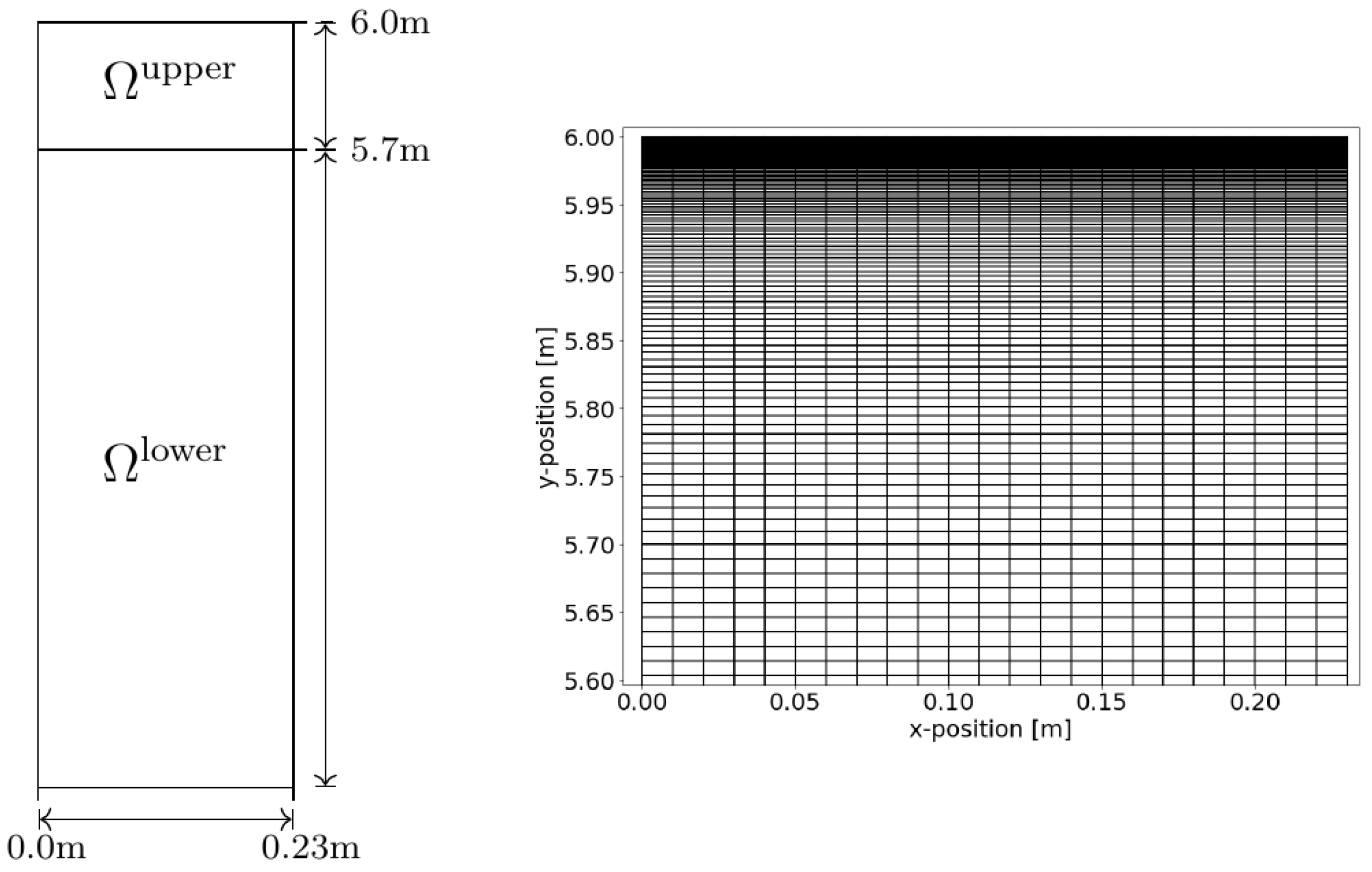
The dimensions of the 2D model domain are assigned to 0.23 m horizontally and 6 m vertically. Velocity is zero at all boundaries. The lateral boundaries as well as the bottom boundary received a Neumann no-flow condition for the mass balance. At the top boundary, the CO2 concentration was prescribed in terms of mole fractions according to the monitored concentrations, which were averaged over time periods of 1 h. Henry’s law was applied to transform cave air partial CO2 pressures into dissolved concentrations in water according to
x CO 2 ( t ) = H w CO 2 · p g CO 2 ( t )
where x CO 2 ( t ) is the mole fraction of CO2 in water, H w CO 2 denotes the Henry constant for CO2 in [ mol CO 2 / ( mol H 2 O · Pa ) ] , and p g CO 2 ( t ) denotes the partial pressure of CO2 at time t corresponding to the averaged tabulated values from the measurements. Linear interpolation was applied if the current time step was between the time of two tabulated values.
The lower left cell in the model domain received an internal Dirichlet boundary condition to impose the pressure from the monitored atmospheric data, corrected with the hydrostatic pressure:
p ( t ) = p atm ( t ) + ρ w g · H
where p atm ( t ) stands for the time-dependent atmospheric pressure data in the cave, ρ w is the density of water, and H the height of the column.

2.4.2. The Grid

The driving force for density-driven enhanced CO2 dissolution in the column (i.e., a density instability) develops at the gas–water interface. We note that we do not model the gas phase and the CO2 dissolution process at the interface; instead, we assume the water at the water table to be in equilibrium with the gas phase, in which we assume the measured CO2 concentration to be equal to the concentration right above the water table. In order to capture the developing instability fingering, the discretization in space and time at the top of the column needs to be high, as discussed in [13,36]. Accordingly, Figure 4 shows our approach for the grid in this study. The model domain Ω is therefore partitioned into two subdomains: Ωlower reaching from the bottom to a height of 5.7 m and Ωupper enclosing the remaining upper part of the model domain. Subdomain Ωlower was discretized with 23 cells in the horizontal direction and 530 in the vertical direction. Subdomain Ωupper was partitioned similarly to Ωlower regarding the horizontal direction; the number of cells in the vertical direction was 100, with a grading factor of 1 / 1.03 for the height of every cell with respect to its cell below.

3. Results

3.1. Data from Long-Term Monitoring

Figure 5 compares daily precipitation and temperature data with the measured curve of the CO2 levels in the cave air. A few distinct features deserve attention. First, let us focus on the precipitation pattern in 2021 and the corresponding strong increase of CO2 in the cave in late summer 2021. The increase of CO2 started with the onset of rain. The following relatively high precipitation paired with summer temperatures likely caused strong microbial activity with potentially high amounts of CO2 in the soil [39,40,41]. It follows a very dry period later towards the fall of 2021. However, the CO2 concentration inside the cave kept rising until the end of August 2021. In 2022, however, there was very little precipitation throughout the summer, unlike the summer of 2021, and microbial activity was likely reduced compared with the year before. The observed peak concentrations in cave air CO2 were smaller in 2022.
Figure 5 shows that precipitation events coincide during certain periods with sudden changes in measured CO2. The rapid drop of CO2 concentrations in March 2022 began during a very dry period in the late winter/early spring. In April 2022, increasing and decreasing CO2 values correlate with precipitation events. The two major rainfall events in April also coincide with spikes in the CO2 curves. In the dry summer of 2022, the CO2 curve fluctuated more than in the previous summer. Although the data are not sufficient to allow for reliable statistics, they indicate that there is a link between precipitation, seasonality, and temperature to CO2 levels inside the cave.
Figure 6 summarizes the data collected from our setup in the cave. The monitoring started in May 2021. Prior to the start of the measurements, the water column was stripped with cave air, which had a CO2 concentration on the order of 15,000 × 10−6 [mol/mol]. In hindsight, this can be classified as an already high initial loading with CO2 in the water. Assuming equilibrium between gaseous and aqueous CO2 to be calculated with Henry’s law, the yellow curve in Figure 6 represents the data of gaseous CO2 concentration in the air above the water table. Note that the values are converted to equivalent aqueous concentrations at the given pressure and temperature conditions. The yellow curve can thus be interpreted as the boundary condition for the CO2 dynamics in the water column. The curves in green and purple show the aqueous CO2 concentrations in 1 m and in 5.85 m water depth, respectively. The data for the control measurements in October/November 2022 are added in the same colours, accordingly. The data logger had a few outages in between. For the numerical simulation, we interpolated linearly where data are missing. Data from water analyses during the control measurement campaign in October/November 2022 are given in Table 1.
Remarks on the measured data:
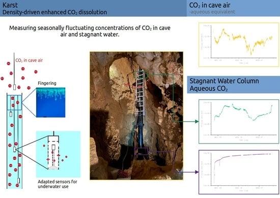
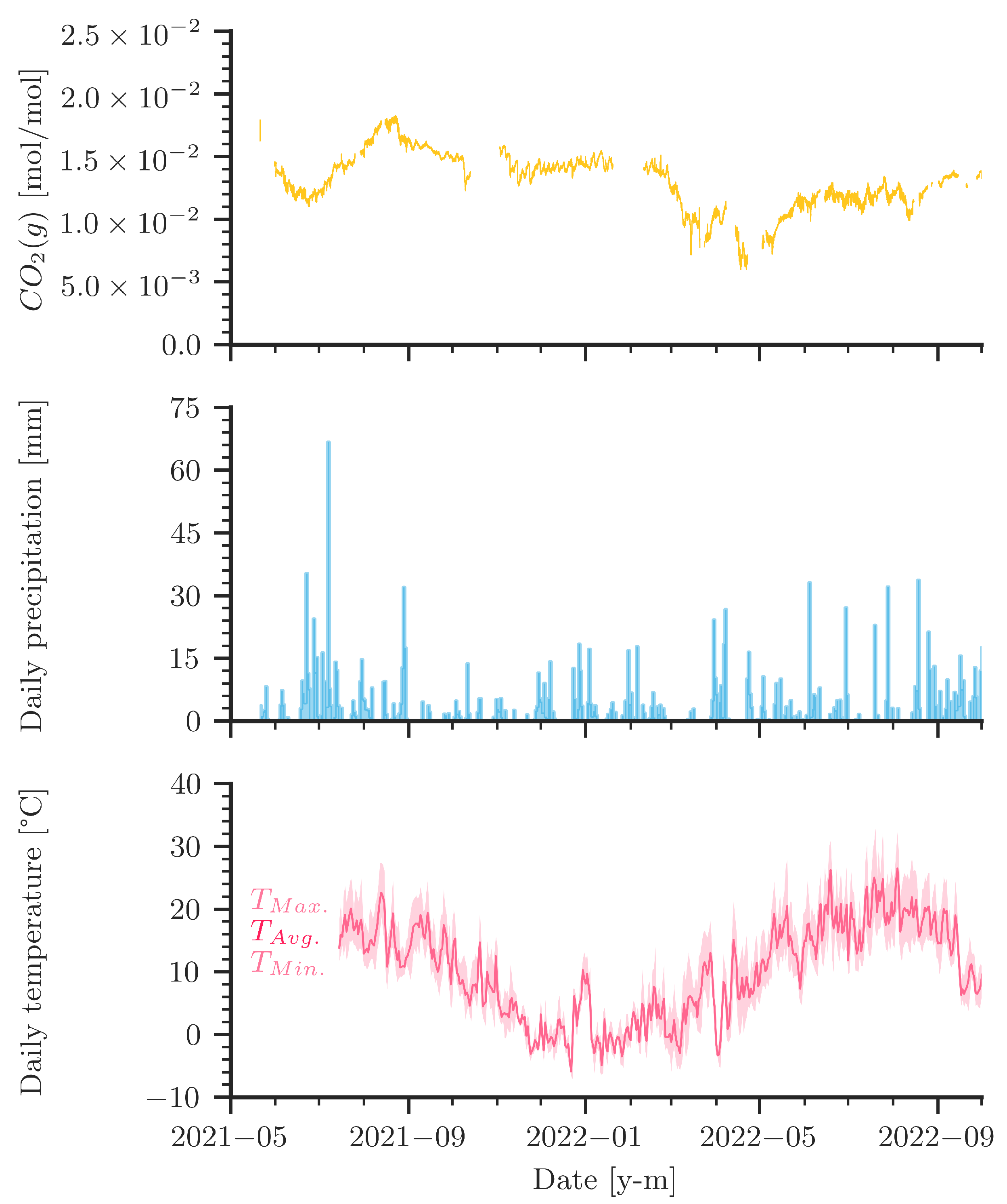
  • The CO2 concentration in the cave’s atmosphere was, as expected, higher in summer than in winter. However, the late-summer peak values in 2021 and 2022 were notably different. Furthermore, a remarkable low was reached around March 2022, followed by a rise that started around April/May 2022.
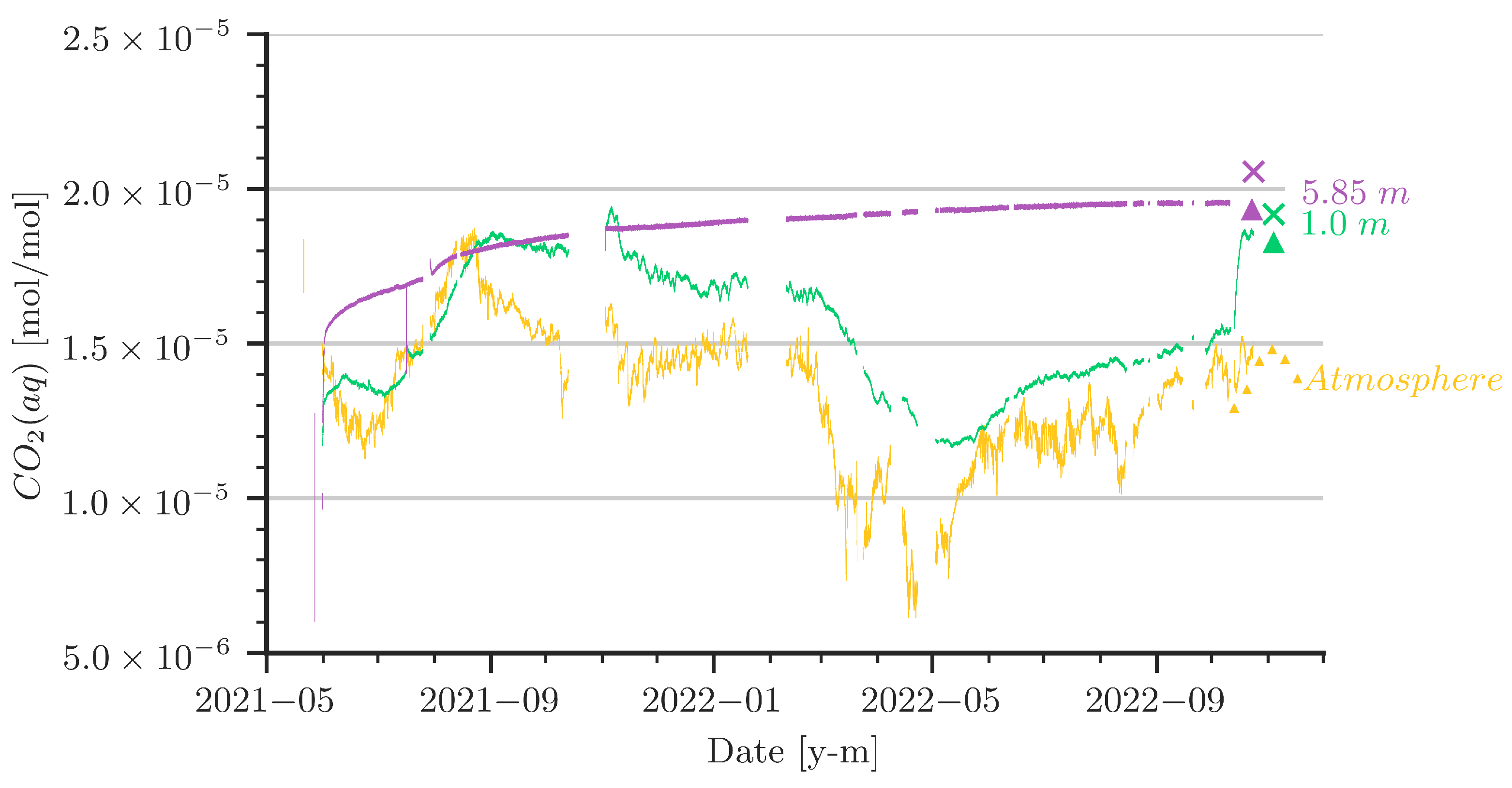
  • It is obvious that the sensor at the 5.85 m depth did not recognize the CO2 concentration dynamics in the cave air, whereas at the 1 m depth there was a clear trend indicating that the aqueous CO2 concentration followed the cave-air concentration.
  • In June/July 2021, a strong increase in the cave-air concentration was followed by an increase of almost the same slope and peak value at the 1 m water depth. As the water is stagnant, the only process to drive this increase is convective mixing (i.e., density-driven enhanced dissolution). During the same time, the CO2 concentration at the 5.85 m depth increased, although with a smaller slope.
  • Let us focus on the period between March and May/June 2022: there, we observe a strong low in the atmospheric CO2 concentration, which was followed with a small delay by the sensor at the 1 m depth, although the low is less pronounced. In a stagnant water column, we would expect only diffusion to be relevant for the release of CO2 from the water back to the atmosphere. However, as diffusion is an extremely slow process with characteristic time scales of several years related to distances of about 1 m, there has to be some small perturbation of the water in the shallower parts of the water column. We will discuss this later.
  • The strong increase of the CO2 concentrations at the 1 m depth (green curve) in October 2022 can be explained by strong perturbances due to our activities during the control measurement campaign. It appears that a mixing was induced while removing the damaged sensor from the 5.85 m depth, which raised water of higher concentration from deeper regions. We decided to include these data in the plots, as they further strengthen confidence in the accuracy of our setup.
  • The control measurement campaign with independent sensors and water samples demonstrated that the sensors used for long-term monitoring were in good agreement with the new sensors. In addition, CO2 concentrations obtained by direct sensor measurements agree with the CO2 concentrations calculated from TIC of water samples.

3.2. Comparison with Numerical Simulations

For the comparison of the measured concentration data with the simulation results, we calculated volume-averaged concentrations from simulation data in the respective heights of the sensors. In addition to the model setup as described in Section 2.4, we attempted to improve the agreement between model and data in a number of variations, two of which are presented in the following. We note that the variations are modifications with no direct physical equivalence. One variation is referred to as ‘Super-Diffusion’; here, the molecular diffusion coefficient in the uppermost centimeter is increased by a factor of 25. A second variation is denoted as ‘Pulses’, where some perturbation is induced during one hour per day; see further below.
Figure 7 and Figure 8 shows that, unfortunately, none of the simulations could match the dynamics of the measured CO2 data satisfactorily. Two major features are seen in the measured curves but are quantitatively not well captured in the simulations:
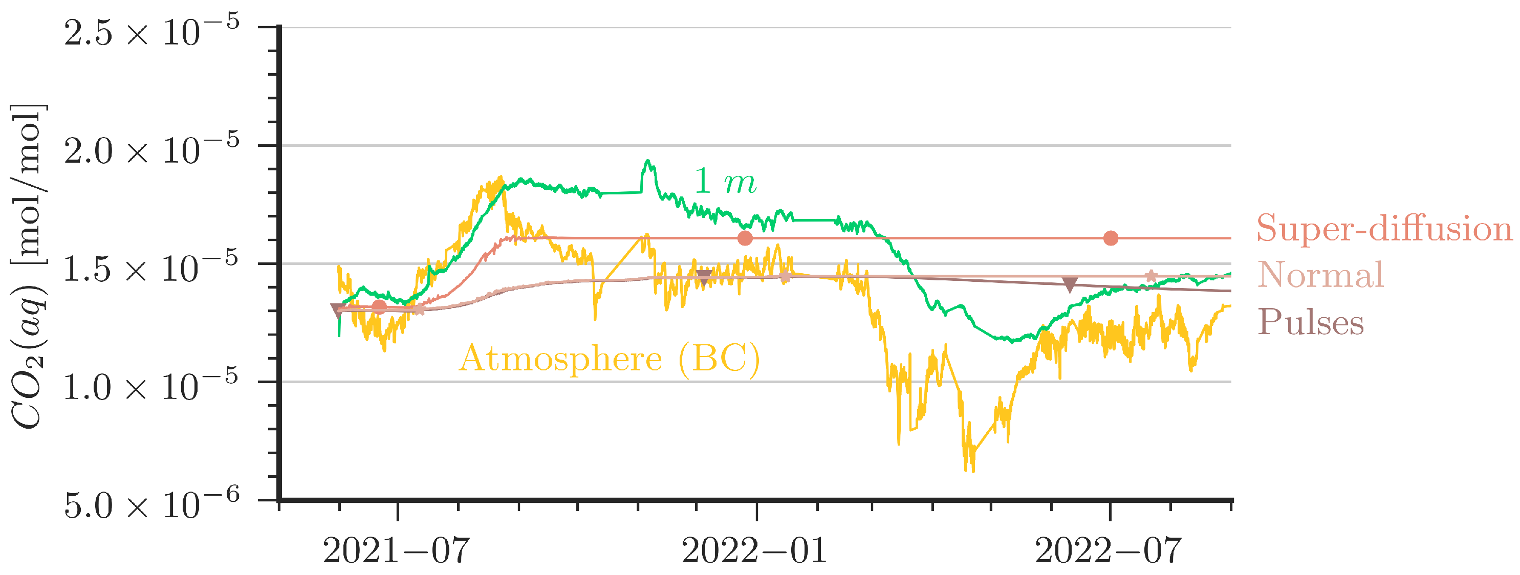
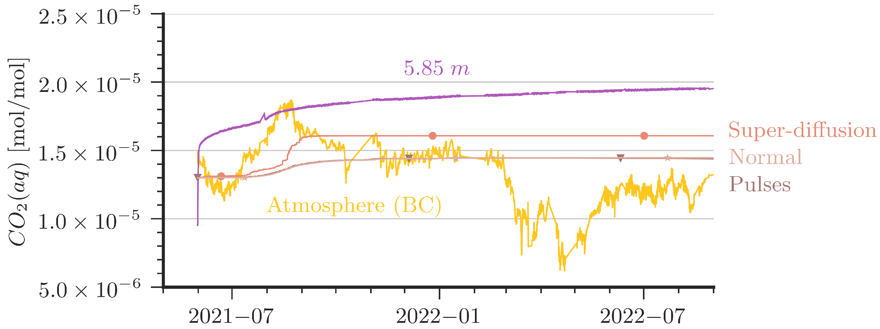
  • The slope of the increase of CO2(aq) after an increase of CO2 in the cave air (e.g., the period from June 2021 to September 2021) is stronger in the measured data than predicted by the simulations. The ‘Super-Diffusion’ scenario is closest to match the slope.
  • The shallower sensor at the 1 m depth shows sensitivity to periods of low cave-air concentrations (e.g., from May 2021 to June 2021 or from March 2022 to May 2022). This could not be reproduced by the simulations except for cases with artificially created perturbation as in the ‘Pulses’ scenario.
The ‘Super-Diffusion’ case is capable of reproducing the slope during CO2 entry periods better than the reference scenario. Obviously, ‘Super-Diffusion’ is not the physical truth, but it demonstrates clearly that the entry rates of CO2 are effectively underestimated. Further grid refinement and smaller time steps cannot substantially improve this mismatch. A contribution to the disagreement is very likely also due to the 2D simplification of the model domain. We provide some remarks on grid convergence and 2D/3D assumptions in Appendix C. In essence, contour plots of CO2 concentrations in the column (see Figure A6) reveal that the entry rates of CO2 at the top are affected by convection cells that look like vortex cascades. These cells reduce the concentration gradient at the top of the water column and, thus, the CO2 entry rates. This may explain to some extent the smaller slope of the increase at the 1 m depth and the very delayed arrival of CO2 at the simulated depth of 5.85 m.
The ‘Pulses’ case can be interpreted as a very slight shaking of the column, which is introduced in the model with a small source term in the momentum equation for one hour per day (0.005 N/m3). For details of the implementation, we refer to the published simulation scenarios [42]. In essence, the ‘Pulses’ cause a small perturbation in the water body such that water with higher CO2 concentration reaches the water table, where CO2 can be released during periods of low cave-air concentration. Diffusion alone would be orders of magnitude too slow to explain the observed decline in CO2 concentration at the 1 m depth, but even tiny driving forces such as in the ‘Pulses’ scenario or, alternatively, tiny temperature fluctuations can already explain the measured curve at the shallow depth (here, 1 m) reacting to the atmospheric concentration.

4. Discussion

4.1. Research Focus of the Study

The motivation for this study is based on previous work that focused on the role of density-driven enhanced dissolution of CO2 in phreatic karst systems. It is important to understand the interaction of elevated and seasonally fluctuating CO2 concentrations in the vadose zone with dissolved CO2 concentrations in phreatic karst water. Density-driven dissolution of CO2 is a relatively slow, vertically oriented process, and it was previously shown that it is promoted by very small lateral advection velocities up to the order of 1 m/day, whereas it is suppressed by stronger advection [13,43]. Thus, the focus on stagnant water in this work is highlighting the favorable conditions for density-driven CO2 dissolution to occur and, more importantly, keeps the required complexity for well-controlled experimental conditions at a minimum.

4.2. Encountered Challenges

Both the experimental part and the numerical simulations turned out to be challenging, for different reasons. Regarding the monitoring, the major unknown prior to the experiment was how long and reliably the employed monitoring method with commercial gas sensors and their adaption to underwater deployment would work. Previous employment of the sensors in the study of [13] covered a period of only two months. They were now applied for a period of 1.5 years until the membrane of the deepest sensor at the 5.85 m depth became leaky during the control measurement campaign, at which time this sensor had to be removed.
For reasons that could not be identified clearly, the data-acquisition system had a few short outages, which lasted, in rare cases, up to more than two weeks until they were detected and repaired. Note that the location in the cave is very remote, and it took time in some instances for detecting the problem and repairing it. This leaves some gaps in the data that were bridged by interpolation for obtaining a continuous time series that was used as input data in the numerical modelling. The overall picture of the seasonal fluctuations is not significantly affected by that. Although a few peaks in the cave-air concentration may have been missed, the measured data in the water reacted more slowly and, dependent on depth, with significantly smaller amplitudes.
In this study, the CO2 sensors were adapted for underwater use by applying a PVC membrane cover. However, the sensor from 5.85 m depth, recovered after its failure, showed some wetting of the inner sensor chamber. We assume that either diffusion of water vapour in the course of the long standing time in water or accidental damage during handling of the control CO2 sensor in the water column had caused the leakage. Nevertheless, the recovered PVC-based membrane appeared to be less ductile than pristine material. We assume that prolonged cold conditions and the release of polymer softener from the PVC membrane increased the PVC brittleness [44].
Interpretation of the Data in the Experimental Column The measured curves are at least qualitatively fully plausible. Regarding quantitative accuracy, the control measurement campaign in October/November 2022 with an independent commercial setup confirmed a 5–10% accuracy in the absolute value, while the fluctuations in concentrations are captured very well and in excellent agreement by all sensors. Thus, we are confident that the observed concentration curves in both water depths are reliable.
Comparing the measurement of the gaseous CO2 concentration in cave air with the measured dissolved concentration at the 1 m depth, the qualitative trend is that the measurement at 1 m water depth always follows the gaseous concentrations with some time delay. The increase of concentrations in the water during periods of highly elevated CO2 concentrations in the air is rather rapid due to the density-driven enhanced dissolution of CO2. The mass balance of CO2 suggests a maximum entry rate of CO2 by dissolution into stagnant water on the order of 0.5 to 1 g CO2 per month and square meter water surface (observed in the summer of 2021).
The decline of CO2 concentrations in the water during times of CO2 lows outside is small but higher than may be expected in perfectly stagnant water, as the dissolved CO2 leads to a stable layering in the water, with the higher concentrations in deeper regions. Thus, diffusion alone, which is many orders slower than density-driven fingering, is not sufficient to explain the decline at the 1 m water depth during the low-CO2 periods in cave air. Obviously, the only possible explanation is that the layering in the water column is not perfect but has small perturbances that affect the shallower parts of the water body.

4.3. Comments on the Link between Cave Air CO2 and Precipitation Data

Our measurements of CO2 in the atmosphere and the precipitation data from DWD support the hypothesis that periods of high and low mobility of CO2 in the gas phase alternate in the course of the year. CO2 concentrations in the cave atmosphere are influenced by a complex interplay of seasonality, precipitation, soil moisture, and soil temperature, and our so far fragmentary understanding demands for more data (e.g., wind measurements in the cave system). It is known that percolating water can transport dissolved inorganic carbon from the canopy of a karst system into facies where the water is stored for a certain amount of time (several years according to [27]), during which it can equilibrate with the gas phase (cave air). Recharge into this storage simultaneously mobilizes water from it; Ref. [27] refers in this context to a piston flow effect; see also Section 2.1. Our hypothesis is that, upon precipitation events, this effect releases (drip) water into the cave in equilibrium with the yearly averaged gas-phase CO2 concentration. We may see an effect of this mechanism between February and May 2022.
We hypothesize another effect from intermittently increased mobility of CO2 in the gas phase during dry periods, which may promote both lows in the cave-air CO2 concentrations in winter and highs in summer. In the summer, the ventilation in the cave tends to be downward oriented, as the cave is colder than the air outside, which would stimulate a net transport of CO2 from the soil layer into the cave (e.g., the high CO2 values in late summer 2021). The opposite would hold in the winter, where ventilation is upwards oriented by trend, and CO2 in the cave air would tend to be diluted (i.e., see the strong low of CO2 values during the extremely dry months of March/April 2022). Ref. [16] presented a simple model where permeable karst fractures facilitate vertical gas exchange. We may also assume that above the large void volumes of the caves there can be small fissures reaching just below the ground surface; they may be covered by a layer of soil on top, which can, dependent on soil moisture, impede (i.e., wet soil) or facilitate (dry soil) gas exchange with the atmosphere. Although the situation is most likely far more complex than this simple model (e.g., ventilation patterns in the cave are not considered so far), our data would support that similar processes do indeed occur.
Further research is required to more thoroughly interpret these coupled phenomena in an interdisciplinary approach including soil science, speleology, and hydrogeology. In any case, this study further strengthens the claim that mobility of CO2 in the soil paired with density-driven dissolution of CO2 may be a carbon-cycle-relevant process beyond the scope of karst science. Density-driven CO2 dissolution may so be one of the ‘unrecognized processes hidden below’ about which is written by [45], who stated in their study on CO2 balances in a desert (i.e., in extremely dry soil!) that ‘a downward CO2 flux seems to have nowhere to go’.

4.4. The (Dis-)Agreement between Data and Numerical Simulations

Different reasons are supposed to contribute to the unsatisfactory match between simulation results and measurements. (i) As noted above, diffusion alone is by far too slow to explain the periods of declining CO2 concentration at the 1 m water depth. Tiny perturbances are sufficient in the model to induce an agitation of the water such that higher concentrations can reach the water table and release CO2 there. This can be due to small temperature fluctuations or tiny vibrations, which we modelled with ‘pulsed’ forces or by superposition of a sinusoidal function of ≈0.0001 g to the gravity vector (the latter was not shown in the results). The accuracy of the measured temperature data did not allow for a quantification of possibly occurring small fluctuations; see Appendix A. (ii) The reason for not matching the CO2 entry rates during periods of high CO2 is much more difficult to identify. We tested grid refinement (Appendix C.1) and time-step refinement, also at the hand of smaller model domains. In the end, none of these approaches allowed for a conclusive assessment. We hypothesize that modelling a 3D experiment in 2D could be a major cause for mismatch. In contrast to the study of [13], where the density differences in the water column were significantly higher and the match between the simulations and the measurements much better, we observe in the model here a distinct fingering regime only in the uppermost part of the column, whereas vertical down-flow in fingers mainly concentrated on the lateral sides of the domain. Further, in particular in the 2D simulations, it appears that a dominant influence of vortex cascades can occur, which we were not able to identify in the physical water column with the given measurement setup. In 3D, the ratio of perimeter to cross-sectional area could favor vertical migration at the walls and also reduce the dominance of vortex cascades. Unfortunately, 3D modeling on the spatial and temporal scales of this experiment is beyond the capabilities of our current model.

5. Conclusions

  • Seasonal fluctuations of gaseous CO2 concentrations in cave air correspond with the concentrations of dissolved CO2 in stagnant water. With increasing depth, this correspondence diminishes. Although it was pronounced at a 1 m depth, there was, practically speaking, no effect anymore at a depth of 6 m.
    It can be concluded that deep water bodies under stagnant or close-to-stagnant conditions can act as efficient traps for CO2 after density-driven dissolution. It remains to be studied in future research how often such conditions are found in real karst settings to assess the relevance of this process for speleogenic theories in comparison to the classical processes relying on water flow.
  • To the authors’ knowledge, this is the first time that the dynamics of CO2 at the gas–water interface and in different depths of a water body were monitored and modelled for real vadose conditions in a cave. It is therefore significant to note that the recognition of stagnant water bodies in caves to be efficient traps for CO2 stands on a solid basis.
  • The data confirm quantitatively that under certain conditions (i.e., soil moisture, temperature, summer/winter), spikes in the concentrations of CO2 in the cave atmosphere coincide with periods of high precipitation. We observed a particularly strong high of CO2 in the cave air in late summer and early fall of 2021. We believe there is strong indication that this was the result of a relatively wet summer followed by an extremely dry period. Low soil moisture facilitates gas exchange between the cave and the soil and high soil-air CO2 concentrations can be transported into the karst system via gas-phase advection and dissolve at the water table.
  • The comparison between the measured CO2 concentrations and numerical simulation results showed qualitative agreement, but the match is not satisfactory. The model predicted significantly smaller entry rates during periods of high air concentrations. In addition, the periods of low air concentrations, where the measurements show a decline also at the 1 m water depth, were (as expected!) not well matched by the model. Different reasons are discussed above and in Appendix C. Tiny perturbances are sufficient to improve the agreement for the declining CO2 concentration at the 1 m depth, although we were unable to determine their origin. A better match of the entry rates is expected for 3D simulations with high spatial and temporal resolution. Modellers with required capabilities are encouraged to use our datasets.
  • Thin PVC-based membrane covers of CO2 sensors are well suited for short-term CO2 observations in water and guarantee a fast response time of the sensor. For time spans exceeding several months or years, material alterations and water vapour diffusion must be considered. To improve long-term stability and accuracy, silicon-based membrane covers might be an appropriate alternative.

Author Contributions

Conceptualization, H.C., B.S. and M.Z.; methodology, H.C., L.K., B.S. and M.Z.; writing—original draft preparation, H.C., L.K., L.S., K.W. and B.S.; writing—review and editing, H.C., B.S. and M.Z.; funding acquisition, H.C.; data curation, L.K., L.S. and K.W.; visualization, L.K. and K.W.; investigation, H.C., L.K. and K.W.; software, L.K. and K.W. All authors have read and agreed to the published version of the manuscript.

Funding

A large part of this research was funded by the German Research Foundation, DFG, under different grants: within the Cluster of Excellence SimTech, grant number 390740016, within Project C04 of the Collaborative Research Center 1313, grant number 327154368, and under grant number 508470891. Significant financial support was also contributed from internal funds by the University of Stuttgart and the GFZ German Research Centre for Geosciences, Potsdam.

Data Availability Statement

The data are available as a dataset hosted at the data repository of the University of Stuttgart (DaRUS) [25]. The code is available as a dataset hosted at the data repository of the University of Stuttgart (DaRUS) [42] and as a DuMux-pub module https://git.iws.uni-stuttgart.de/dumux-pub/class2023a, accessed on 2 February 2023.

Acknowledgments

The experimental part of this work is strongly based on a preliminary study at the University of Stuttgart, and we thank Pascal Bürkle and Oliver Trötschler for their help. Harry Scherzer (Höhlen- und Heimatverein Laichingen) has contributed with his inspiring ideas. Patrizia Ambrisi helped us designing the graphical abstract.

Conflicts of Interest

The authors declare no conflict of interest.

Abbreviations

The following abbreviations are used in this manuscript:
LWZweckverband Landeswasserversorgung—state water supply to the Laichingen region
DWDDeutscher Wetterdienst—German Meteorological Service

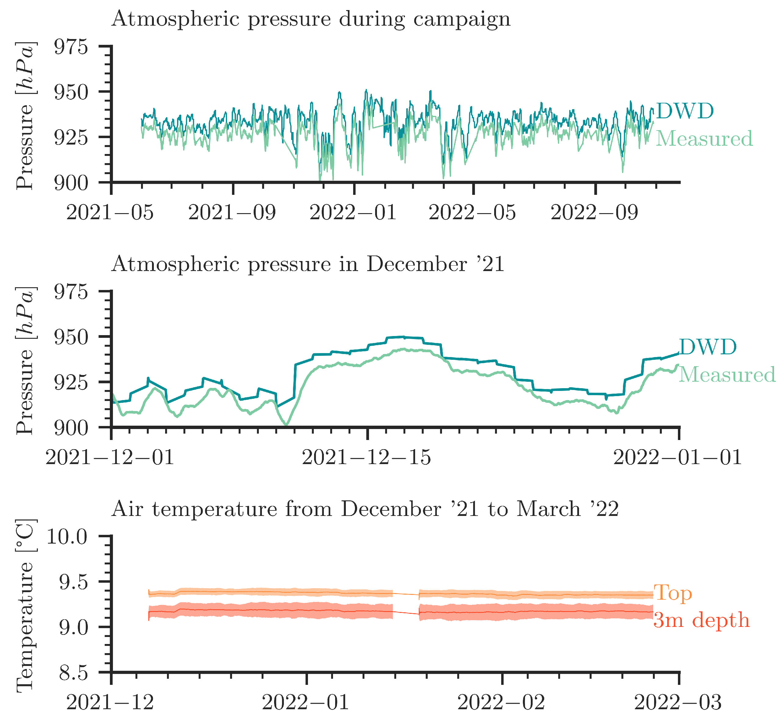
Appendix A. Measured Pressure and Temperature Data

Figure A1 (top and middle) provides details on barometric pressure data from the German Meteorological Service (DWD) in comparison to our own recordings of air pressure in the cave. The plots show an excellent qualitative agreement. The measured atmospheric pressure data are used in the numerical simulations as boundary conditions.
Figure A1. (Top): Comparison of our own measured atmospheric pressure with data from the DWD (“Deutscher Wetterdienst”). The DWD data is from Stötten (at a 25 km distance from Laichingen at almost the same altitude). (Middle): Exemplary detailed view in December 2021. (Bottom): Measured air temperature over time inside the cave; daily moving average and standard deviation. The data shown here are uncorrected raw data from temperature sensors; they indicate that within measurement accuracy the temperature is constant in time. From repeated control measurements (not shown), we have robust confirmation that there is no measurable temperature gradient from the top to the bottom of the column.
Geosciences 13 00051 g0a1
The bottom plot in Figure A1 reports the temperature curves measured with the thermocouples; see also Figure 2. The curves show the daily moving average and the standard deviation. We conclude that the temperature is more or less constant over time, whereas the noise in the data (expressed by the standard deviation) is significantly larger than any temperature fluctuations. Repeated control measurements confirmed that no temperature gradient exists along the column. An assessment of possibly occurring small-amplitude temperature fluctuations is not possible. It is, thus, not possible to use the temperature data to strengthen or to refute the hypothesis of small temperature fluctuations leading to small convective perturbances in the shallow parts of the water column.

Appendix B. Details on the Governing Model Equations

The continuity equation for each component κ {H2O,CO2} is written as
ϱ X κ t + · ϱ v X κ D κ ϱ X κ = 0 ,
where ϱ represents the density of the aqueous phase and depends on the concentration of CO2, here expressed by the mass fraction X. The velocity vector is denoted by v; D is the binary diffusion coefficient.
As the density model and measurements use mole fractions, the simulation was conducted using mole fractions. The conversion between mass and mole fraction can be written as
X κ = x κ × M κ κ x κ × M κ
The Navier–Stokes equation to describe momentum transport is written as
( ϱ v ) t + · ( ϱ v v T ) = · ( μ ( v + v T ) ) p + ϱ g ,
with μ representing the dynamic viscosity and g the gravitational acceleration vector.
This model uses as primary unknowns the pressure, the concentration of CO2 in terms of a mass fraction of the water phase, and the vector of velocity. The equations are solved on a staggered grid. This means that pressure and concentrations exist in a control volume, which is staggered from the control volume where the velocity components exist. The staggered scheme prevents pressure oscillations and is mass conservative. The equations are solved fully implicitly, and non-linearities are addressed by Newton’s method. The convergence of Newton’s method affects the time-step control, and the user can set a maximum time-step size. Because time series of CO2 concentration data at the top boundary conditions are given, the temporal resolution of these data is in fact in our case the constraint for the time-step control.
Following [46], the density (in kg/m3) is computed as
ϱ = 1 x CO 2 V ϕ M T + x H 2 O M H 2 O ϱ w M T
where ϱ w is the density of pure water dependent on pressure and temperature, and M H 2 O is the molar mass (in kg/mol) of pure water; M T is calculated as
M T = M H 2 O x H 2 O + M CO 2 x CO 2 .
The apparent molar volume of dissolved CO2, V ϕ (in m3/mol) is a function of temperature T (in °C):
V ϕ = 1 e 6 ( 37.51 9.585 e 2 T + 8.74 e 4 T 2 5.044 e 7 T 3 ) .

Appendix C. Investigations on Grid Convergence and 2D/3D Assumption

To investigate how the entry rate of CO2 at the top boundary is affected by model choices, we studied the influence of grid refinement and the assumption of a 2D domain.

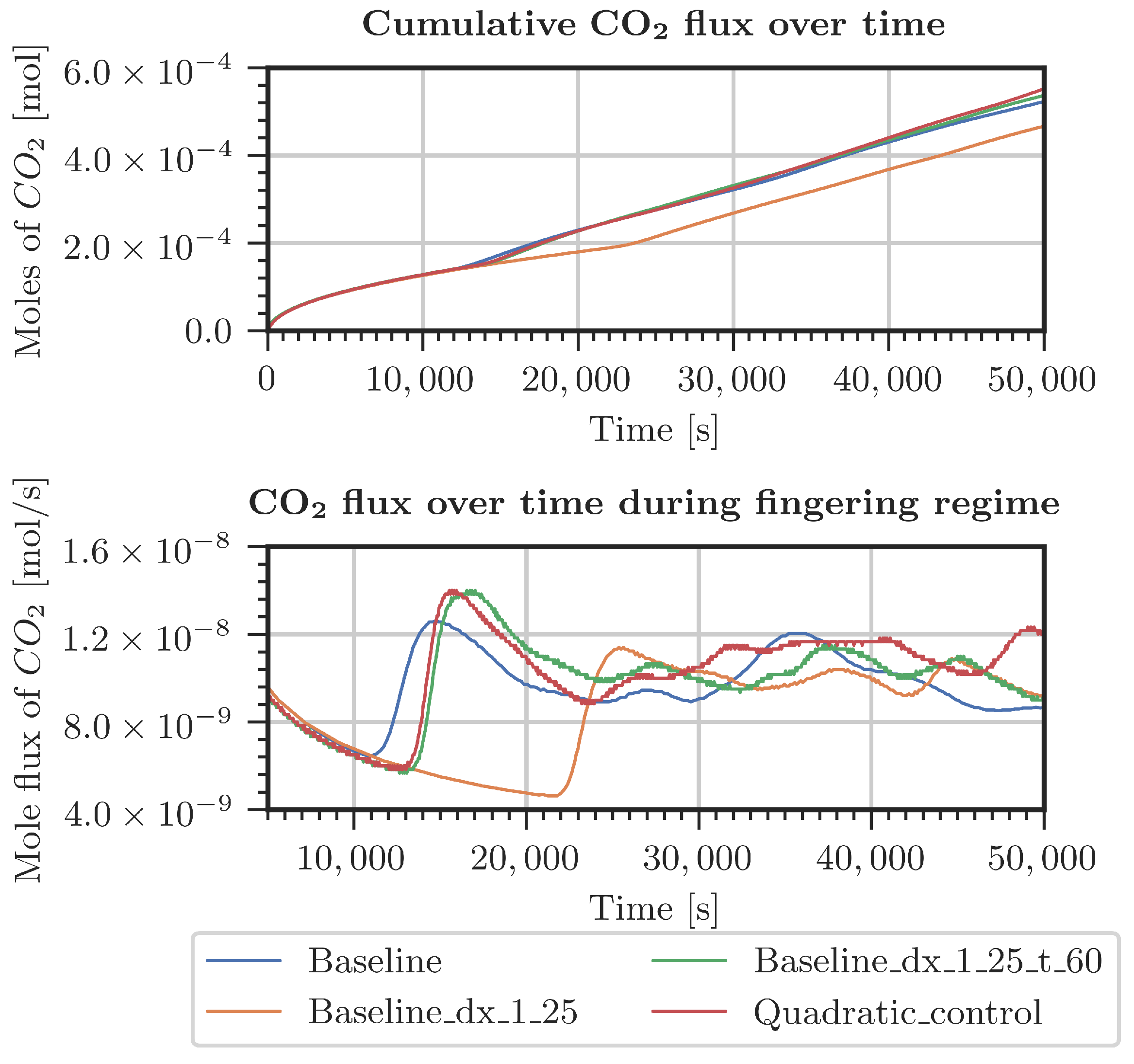
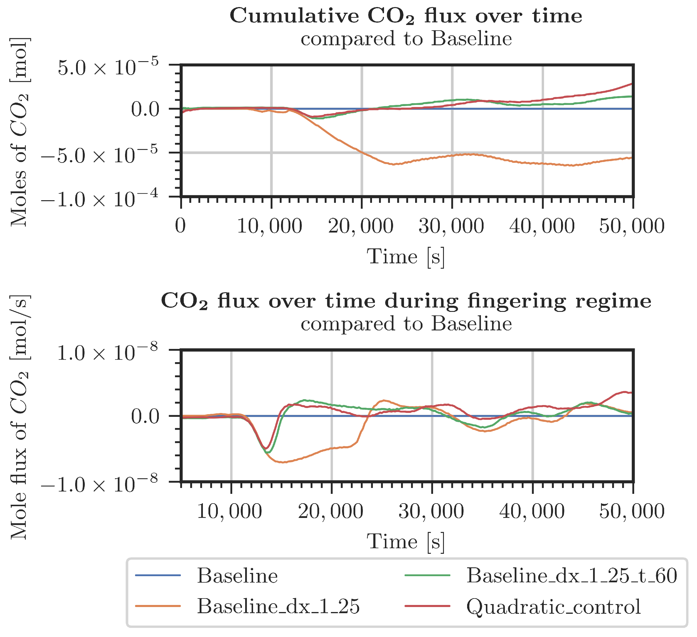
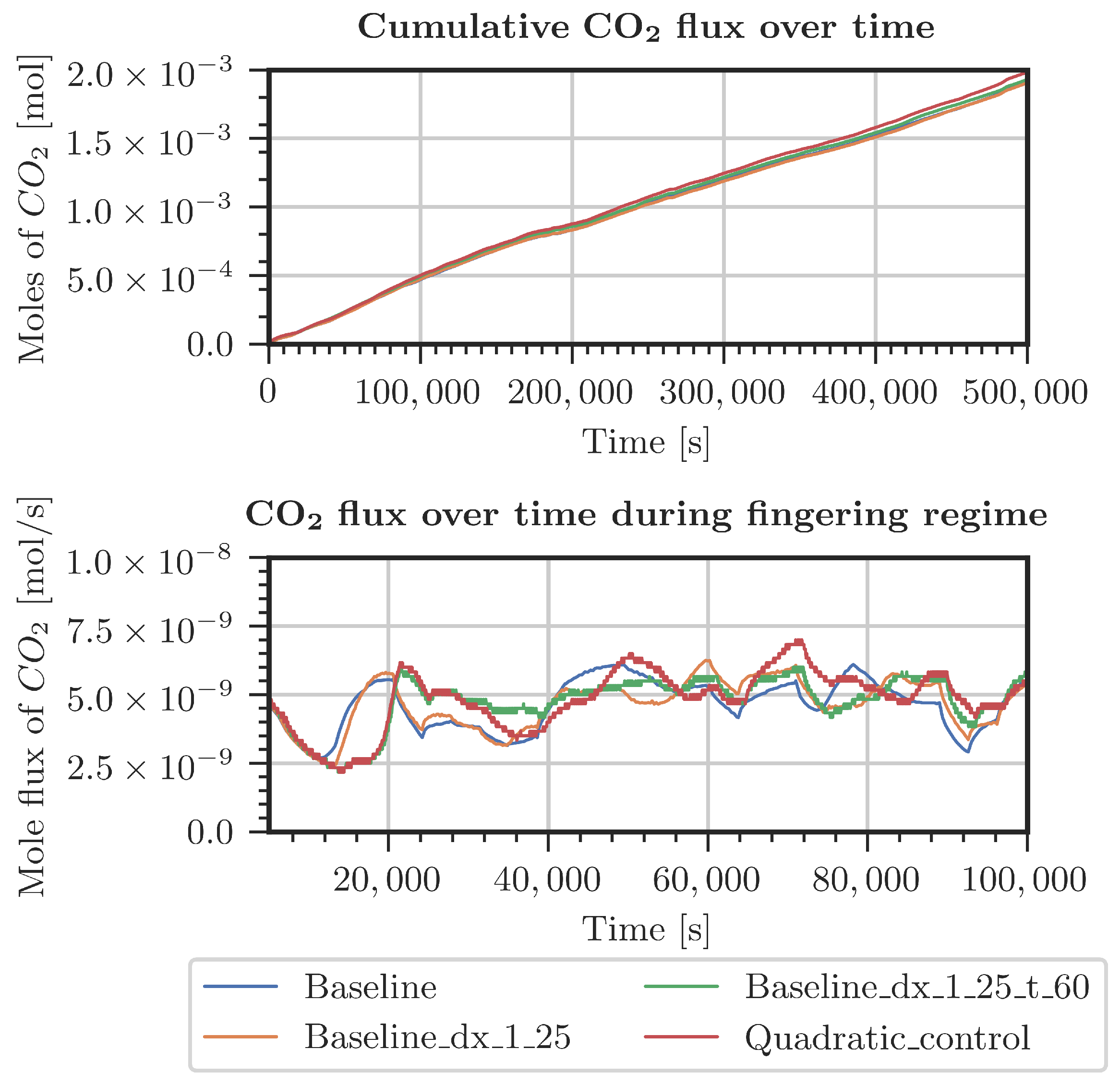
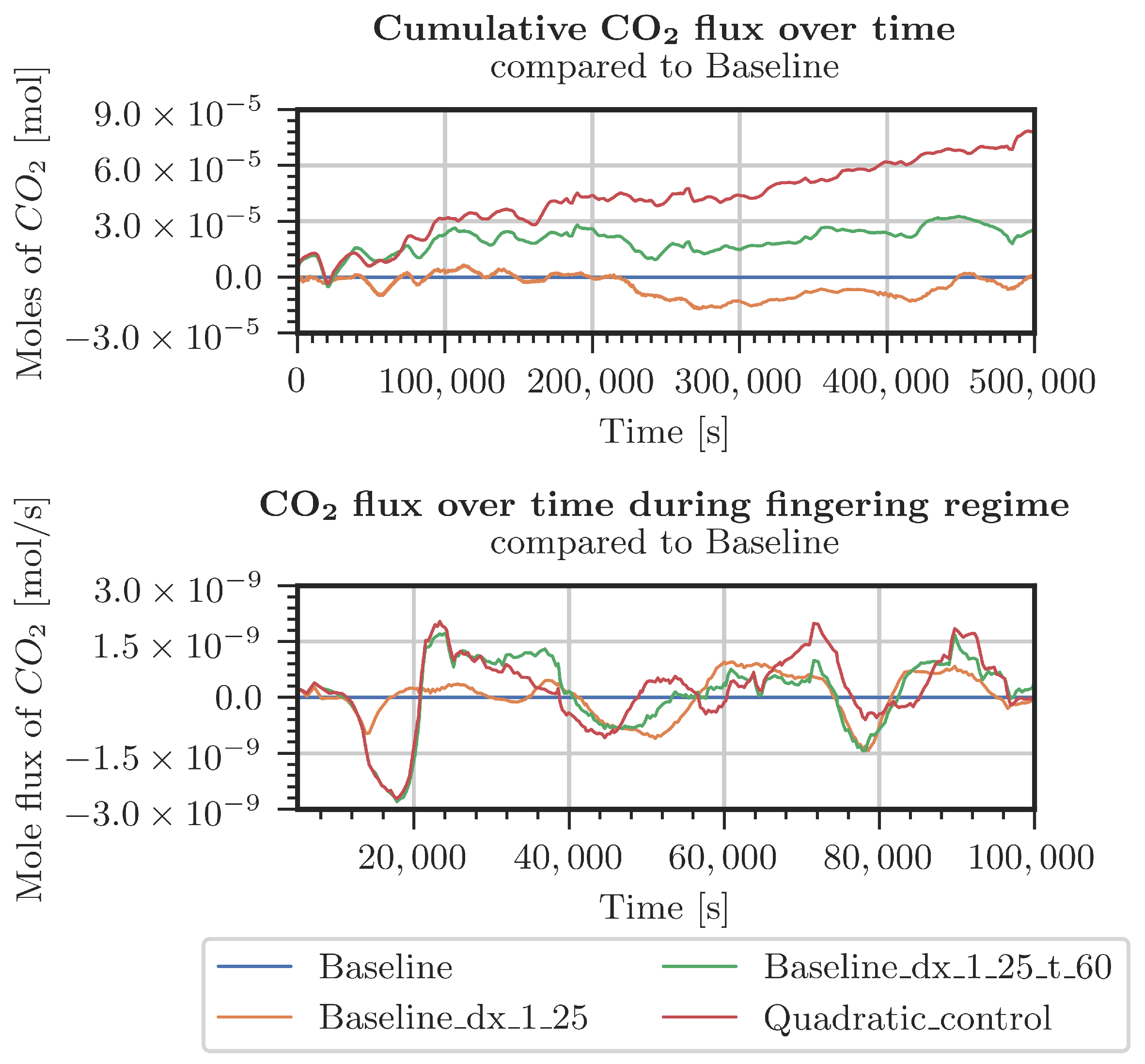
Appendix C.1. Grid Refinement Studies

Table A1. Discretizations used in grid refinement study.
CaseΔ x [mm]Δ y [mm]Grading yΔ t [s]
Baseline103−1.033600
Baseline dx 553−1.033600
Baseline dx 2.52.53−1.033600
Baseline dx 1.251.253−1.033600
Baseline dx 1.25 t 18001.253−1.031800
Baseline dx 1 25 t 601.253−1.0360
Baseline dx 1.25 t 60 dy 1.51.251.5−1.0360
Baseline dx 1.25 t 3600 dy 1.51.251.5−1.033600
Quadratic control t 36001.251.2513600
Quadratic control1.251.25160
Different cases were specified for a refinement study in the top 30 cm of the domain. The first case used pressure and concentrations from the measured data in the period starting from July 2021 (Figure A4 and Figure A5). The second case considered constant pressure and CO2 concentrations at the top boundary of the model domain (Figure A2 and Figure A3). For both cases, the employed grids are shown in Table A1. The grid resolution used in the simulations of the whole domain is denoted as the baseline grid. In general, finer discretization tends to result in a higher inflow of CO2. Onset times of fingering showed a surprising result: the coarsest discretization produced the earliest onset time. This holds true for both kinds of boundary conditions. In conclusion, the grid used for the simulations shown in Section 3.2 is not perfectly grid-converged. Still, the differences are by far not significant enough to blame grid resolution for the slow response of the system compared with the measured data.
Figure A2. Comparison of CO2 entering the system for various grids (Table A1). Constant pressure and CO2 concentration at the top boundary.
Geosciences 13 00051 g0a2
Figure A3. Difference in CO2 entering the system for various grids (Table A1) with respect to the baseline grid. Constant pressure and CO2 concentration at the top boundary.
Geosciences 13 00051 g0a3
Figure A4. Comparison of CO2 entering the system for various grids (Table A1). Measured pressure and CO2 concentration at the top boundary.
Geosciences 13 00051 g0a4
Figure A5. Difference in CO2 entering the system for various grids (Table A1) with respect to the baseline grid. Measured pressure and CO2 concentration at the top boundary.
Geosciences 13 00051 g0a5

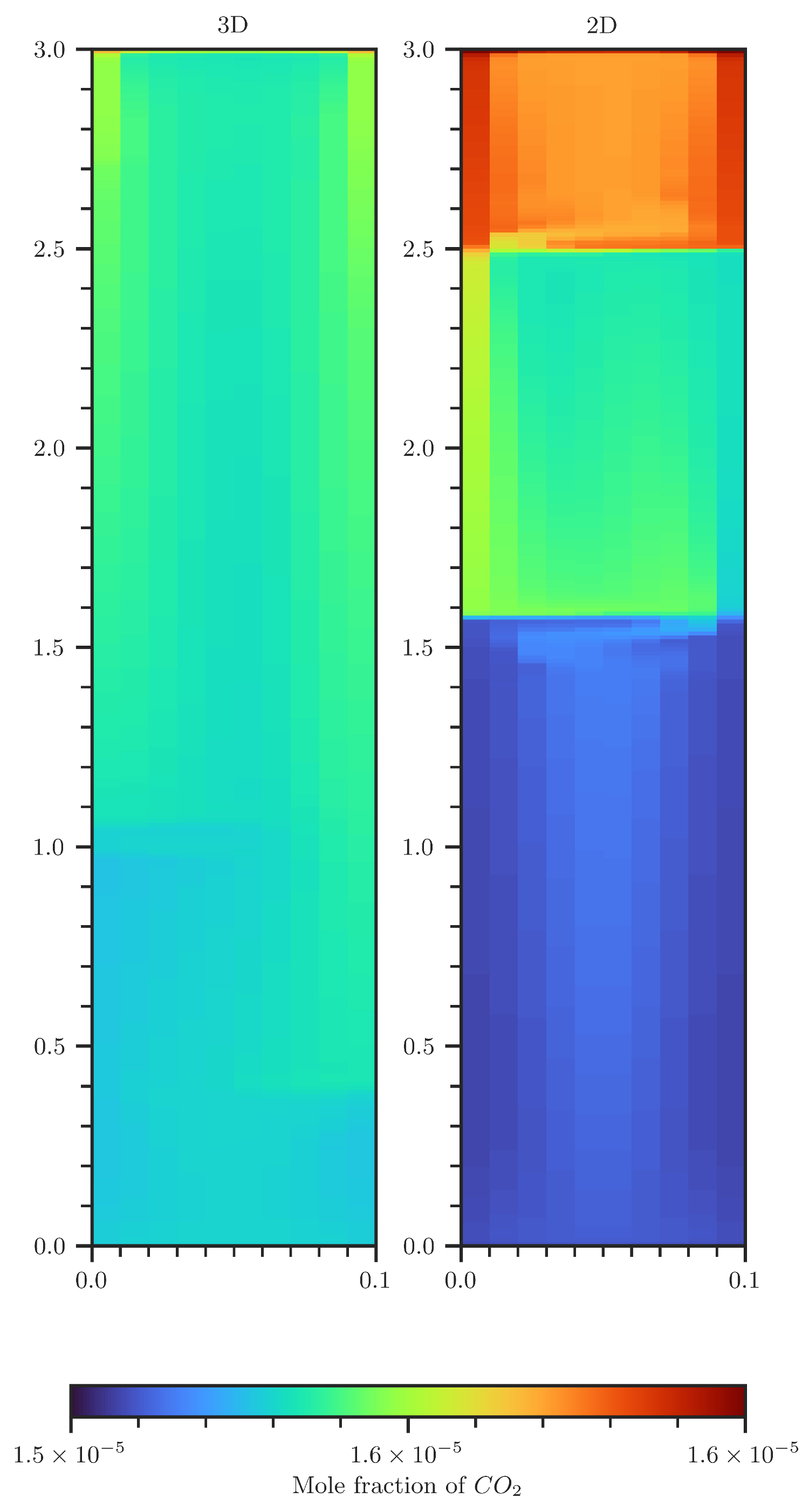
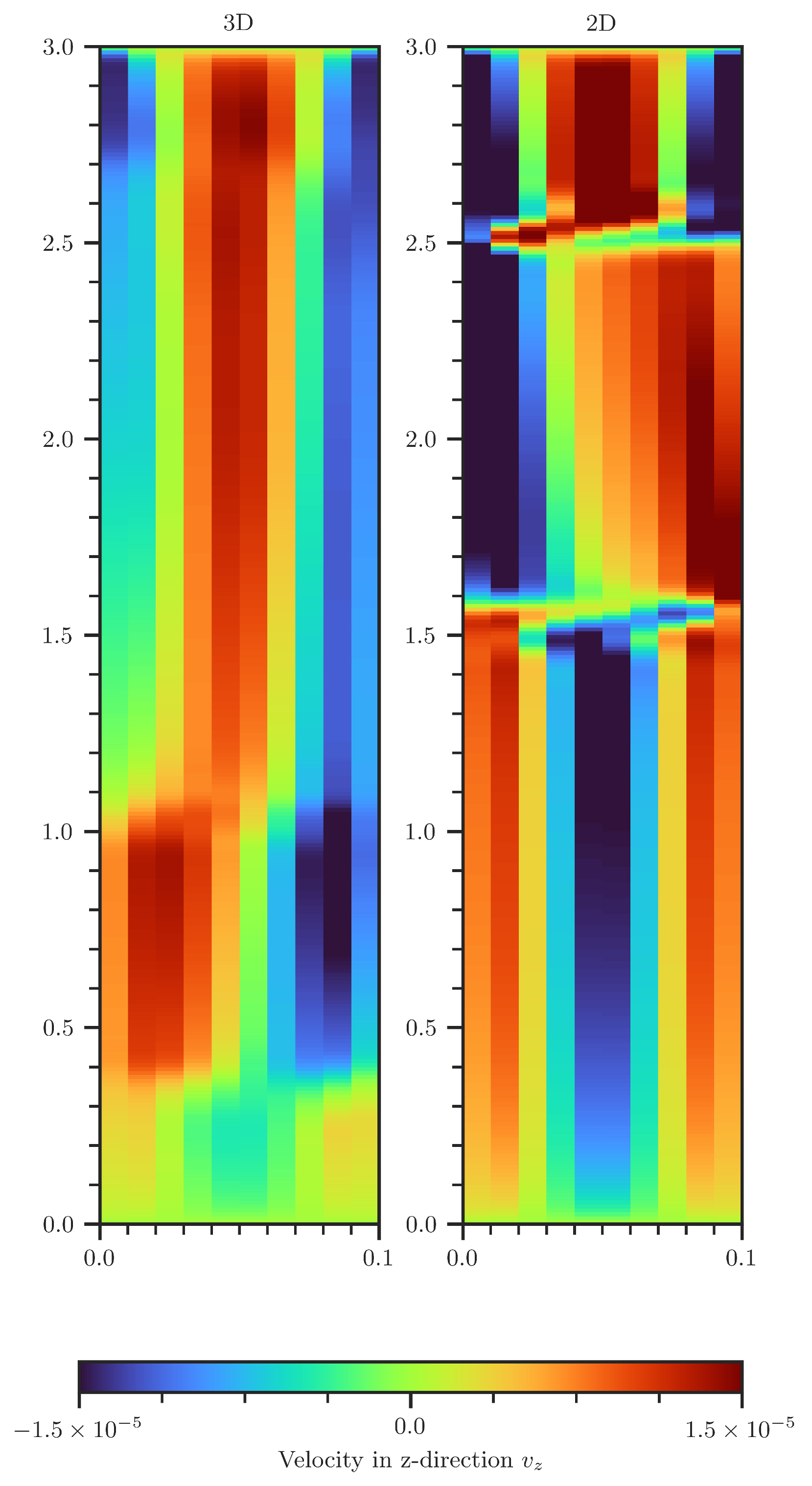
Appendix C.2. Comparison of 2D and 3D Domains

A smaller domain was used to investigate possible differences between 2D and 3D simulations. Of particular interest is the emergence of vortex cascades and the corresponding effects, mainly a possible hindrance of CO2 influx. Both setups have a height of 3 m and a width of 0.1 m. The 3D setup has a depth of 0.1 m, leading to a cross-sectional area of 10 cm × 10 cm. The initial CO2 concentration was set to 15 × 10−6 [mol/mol] with a boundary condition oscillating around 18 × 10−6 [mol/mol] (see Equation (A7)).
x CO 2 ( t ) = 0.5 × 10 6 sin ( 2.424068 · t ) + 18 × 10 6
In the 2D setup, the downward migration of CO2-rich water occurs predominantly at the lateral boundaries. For the 3D setup, the CO2-rich water mostly migrates in the corners of the domain (see Figure A6, the 2D representation of the 3D is due to averaging over the depth). Studying the effects of such corner flow is beyond the scope of this Appendix; it is, however, likely to have an influence. In both setups, the upward migration of less-dense fluid is predominantly in the center of the cross-section.
Vortex cascades formed in both 2D and 3D setups. In the 3D setup, however, they emerge near the bottom of the domain, whereas in the 2D setup, this effect is observed at the upper region of the model domain. For the 3D setup, the vortexes do not cover the entire cross-section. Adding a third dimension allows for denser water to form a helical-like stream into deeper regions (see Figure A7), permitting that upwards and downwards streams can better avoid each other. At earlier times, this is causing a higher CO2 concentration deep inside the column for the 3D setup. One observes that the CO2 flux is 10–20% higher in the 3D domain. Note that a reduced CO2 influx could not be distinctly connected with an occurrence of vortex cascades.
Figure A6. Comparison of CO2 concentration contour plots of a 2D (right) and 3D (left) scenario. The 3D plot shows concentrations that are volume averaged over the second spatial dimension.
Geosciences 13 00051 g0a6
Figure A7. Comparison of vertical velocity in the 2D (right) and 3D (left) scenario. In 3D, the velocities are volume averaged over the second spatial dimension.
Geosciences 13 00051 g0a7

References

  1. Ford, D.; Williams, P. Karst Hydrogeology and Geomorphology; Wiley: Hoboken, NJ, USA, 2007. [Google Scholar] [CrossRef]
  2. Mangin, A. Contribution à l’étude Hydrodynamique Des Aquifères Karstiques. Ph.D. Thesis, Sciences de la Terre, Université de Dijon, Dijon, France, 1975. [Google Scholar]
  3. White, W. Caves and Karst of the Greenbrier Valley in West Virginia; Caves and Karst Systems of the World; Springer: Cham, Switzerland, 2018. [Google Scholar] [CrossRef]
  4. Dreybrodt, W. Processes in Karst Systems-Physics, Chemistry, and Geology; Physical Environment; Springer: Berlin/Heidelberg, Germany, 1988. [Google Scholar] [CrossRef]
  5. Bonacci, O. Karst Hydrology: With Special Reference to the Dinaric Karst; Physical Environment; Springer: Berlin/Heidelberg, Germany, 1987. [Google Scholar] [CrossRef]
  6. Stevanovic, Z. Karst Aquifers-Characterization and Engineering; Springer: Cham, Switzerland; Heidelberg, German; New York, NY, USA; Dordrecht, The Netherlands; London, UK, 2015. [Google Scholar] [CrossRef]
  7. Klimchouk, A.; Ford, D.; Palmer, A.; Dreybrodt, W. (Eds.) Speleogenesis-Evolution of Karst Aquifers; National Speleological Society: Huntsville, AL, USA, 2000.
  8. Bögli, A. Karst Hydrology and Physical Speleology; Springer: Berlin/Heidelberg, Germany, 1980. [Google Scholar] [CrossRef]
  9. Gabrovšek, F.; Dreybrodt, W. Role of mixing corrosion in calcite-aggressive H2O-CO2-CaCO3 solutions in the early evolution of karst aquifers in limestone. Water Resour. Res. 2000, 36, 1179–1188. [Google Scholar] [CrossRef]
  10. Ford, D.; Ewers, R. The development of limestone caves in the dimensions of length and depth. Int. J. Speleol. 1978, 10, 213–244. [Google Scholar] [CrossRef]
  11. Dreybrodt, W. Dissolution: Carbonate rocks. Encyclopedia of Caves and Karst Science; Taylor & Francis: London, UK, 2004; pp. 295–298. [Google Scholar]
  12. Kaufmann, G.; Gabrovšek, F.; Romanov, D. Deep conduit flow in karst aquifers revisited. Water Resour. Res. 2014, 50, 4821–4836. [Google Scholar] [CrossRef]
  13. Class, H.; Bürkle, P.; Sauerborn, T.; Trötschler, O.; Strauch, B.; Zimmer, M. On the role of density-driven dissolution of CO2 in phreatic karst systems. Water Resour. Res. 2021, 57, e2021WR030912. [Google Scholar] [CrossRef]
  14. IPCC. Special Report on Carbon Dioxide Capture and Storage. In Technical Report, Intergovernmental Panel on Climate Change (IPCC), prepared by Working Group III; Metz, B., Davidson, O., de Conink, H.C., Loos, M., Meyer, L.A., Eds.; Cambridge University Press: Cambridge, UK; New York, NY, USA, 2005. [Google Scholar]
  15. Green, C.; Ennis-King, J. Steady flux regime during convective mixing in three-dimensional heterogeneous porous media. Fluids 2018, 3, 58. [Google Scholar] [CrossRef]
  16. Covington, M. The importance of advection for CO2 dynamics in the karst critical zone: An approach from dimensional analysis. In Caves and Karst Across Time; Special Paper 516; Feinberg, J., Gao, Y., Alexander, E., Eds.; Geological Society of America: Boulder, CO, USA, 2016. [Google Scholar] [CrossRef]
  17. Ennis-King, J.; Paterson, L. Rate of dissolution due to convective mixing in the underground storage of carbon dioxide. In Greenhouse Gas Control Technologies; Gale, J., Kaya, Y., Eds.; Elsevier: Amsterdam, The Netherlands, 2003; Volume 1, pp. 507–510. [Google Scholar] [CrossRef]
  18. Ennis-King, J.; Paterson, L. Role of convective mixing in the long-term storage of carbon dioxide in deep saline formations. In Proceedings of the Annual Fall Technical Conference and Exhibition, Denver, CO, USA, 5–8 October 2003; Society of Petroleum Engineers: Richardson, TX, USA, 2003. Number SPE-84344. [Google Scholar] [CrossRef]
  19. Riaz, A.; Hesse, M.; Tchelepi, H.; Orr, F. Onset of convection in a gravitationally unstable diffusive boundary layer in porous media. J. Fluid Mech. 2006, 548, 87–111. [Google Scholar] [CrossRef]
  20. Hassanzadeh, H.; Pooladi-Darvish, M.; Keith, D. Modelling of convective mixing in CO2 storage. J. Can. Pet. Technol. 2005, 44. [Google Scholar] [CrossRef]
  21. Hassanzadeh, H.; Pooladi-Darvish, M.; Keith, D. Stability of a fluid in a horizontal saturated porous layer: Effect of non-linear concentration profile, initial, and boundary conditions. Transp. Porous Media 2006, 65, 193–211. [Google Scholar] [CrossRef]
  22. Emami-Meybodi, H.; Hassanzadeh, H.; Green, C.; Ennis-King, J. Convective dissolution of CO2 in saline aquifers: Progress in modeling and experiments. Int. J. Greenh. Gas Control. 2015, 40, 238–266. [Google Scholar] [CrossRef]
  23. Hassanzadeh, H.; Pooladi-Darvish, M.; Keith, D. Scaling behavior of convective mixing, with application to geological storage of CO2. Am. Inst. Chem. Eng. J. 2007, 53, 1121–1131. [Google Scholar] [CrossRef]
  24. Pau, G.; Bell, J.; Pruess, K.; Almgren, A.; Lijewski, M.; Zhang, K. High resolution simulation and characterization of density-driven flow in CO2 storage in saline aquifers. Adv. Water Resour. 2010, 33, 443–455. [Google Scholar] [CrossRef]
  25. Keim, L.; Class, H.; Schirmer, L.; Wendel, K.; Strauch, B.; Zimmer, M. Data for: Measurement Campaign of Gaseous CO2 Concentrations in a Karst Cave with Aqueous Concentrations in a Stagnant Water Column 2021–2022. Tech. Rep. 2022. [Google Scholar] [CrossRef]
  26. Frank, R. Zur Morphologie der Laichinger Tiefenhöhle. Laichinger Höhlenfreund. 2019, 54, 33–48. Available online: https://www.academia.edu/45140466 (accessed on 22 January 2023).
  27. Selg, M.; Schwarz, K. Am Puls der schönen Lau-zur Hydrogeologie des Blautopf-Einzugsgebiets. Laichinger Höhlenfreund. 2009, 44, 45–72. Available online: http://www.blauhoehle.org/images/pdf/hydrogeologie_blautopf.pdf (accessed on 22 January 2023).
  28. Kjeldsen, P. Evaluation of gas diffusion through plastic materials used in experimental and sampling equipment. Water Res. 1993, 27, 121–131. [Google Scholar] [CrossRef]
  29. Zimmer, M.; Erzinger, J.; Kujawa, C.; CO2-SINK-Group. The gas membrane sensor (GMS): A new method for gas measurements in deep boreholes applied at the CO2 SINK site. Int. J. Greenh. Gas Control 2011, 5, 995–1001. [Google Scholar] [CrossRef]
  30. De Gregorio, S.; Camarda, M.; Longo, M.; Cappuzzo, S.; Giudice, G.; Gurrieri, S. Long-term continuous monitoring of the dissolved CO2 performed by using a new device in groundwater of the Mt. Etna (southern Italy). Water Res. 2011, 45, 3005–3011. [Google Scholar] [CrossRef]
  31. Johnson, M.; Billett, M.; Dinsmore, K.; Wallin, M.; Dyson, K.; Jassal, R. Direct and continuous measurement of dissolved carbon dioxide in freshwater aquatic systems method and applications. Ecohydrology 2010, 3, 68–78. [Google Scholar] [CrossRef]
  32. Strauch, B.; Heeschen, K.U.; Schicks, J.M.; Spangenberg, E.; Zimmer, M. Application of tubular silicone (PDMS) membranes for gas monitoring in CO2–CH4 hydrate exchange experiments. Mar. Pet. Geol. 2020, 122, 104677. [Google Scholar] [CrossRef]
  33. Roy, R.N.; Roy, L.N.; Vogel, K.M.; Porter-Moore, C.; Pearson, T.; Good, C.E.; Millero, F.J.; Campbell, D.M. The dissociation constants of carbonic acid in seawater at salinities 5 to 45 and temperatures 0 to 45°C. Mar. Chem. 1993, 44, 249–267. [Google Scholar] [CrossRef]
  34. Millero, F.J. The thermodynamics of the carbonate system in seawater. Geochim. Cosmochim. Acta 1979, 43, 1651–1661. [Google Scholar] [CrossRef]
  35. Leal, A. Reaktoro: An Open-Source Unified Framework for Modeling Chemically Reactive Systems. 2015. Available online: https://reaktoro.org (accessed on 2 February 2023).
  36. Class, H.; Weishaupt, K.; Trötschler, O. Experimental and Simulation Study on Validating a Numerical Model for CO2 Density-Driven Dissolution in Water. Water 2020, 12, 738. [Google Scholar] [CrossRef]
  37. Koch, T.; Gläser, D.; Weishaupt, K.; Ackermann, S.; Beck, M.; Becker, B.; Burbulla, S.; Class, H.; Coltman, E.; Emmert, S.; et al. DuMux 3—An open-source simulator for solving flow and transport problems in porous media with a focus on model coupling. Comput. Math. Appl. 2021. [Google Scholar] [CrossRef]
  38. DuMux Handbook. Available online: https://dumux.org/docs/handbook/master/dumux-handbook.pdf (accessed on 2 February 2023).
  39. Peyraube, N.; Lastennet, R.; Denis, A.; Malaurent, P.; Villanueva, J. Interpreting CO2-SIc relationship to estimate CO2 baseline in limestone aquifers. Environ. Earth Sci. 2015, 1, 19–26. [Google Scholar] [CrossRef]
  40. Schimel, J. Life in dry soils: Effects of drought on soil microbial communities and processes. Annu. Rev. Ecol. Evol. Syst. 2018, 49, 409–432. [Google Scholar] [CrossRef]
  41. von Lützow, M.; Kögel-Knabner, I. Temperature sensitivity of soil organic matter decomposition—What do we know? Biol. Fertil. Soils 2009, 46, 1–15. [Google Scholar] [CrossRef]
  42. Keim, L.; Class, H.; Schirmer, L.; Strauch, B.; Wendel, K.; Zimmer, M. Code for: Seasonal Dynamics of Gaseous CO2 Concentrations in a Karst Cave Correspond with Aqueous Concentrations in a Stagnant Water Column. Tech. Rep. 2022. [Google Scholar] [CrossRef]
  43. Tsinober, A.; Rosenzweig, R.; Class, H.; Helmig, R.; Shavit, U. The role of mixed convection and hydrodynamic dispersion during CO2 dissolution in saline aquifers: A numerical study. Water Resour. Res. 2021, 58, e2021WR030494. [Google Scholar] [CrossRef]
  44. Ito, M.; Nagai, K. Analysis of degradation mechanism of plasticized PVC under artificial aging conditions. Polym. Degrad. Stab. 2007, 92, 260–270. [Google Scholar] [CrossRef]
  45. Ma, J.; Lio, R.; Tsang, L.S.; Lan, Z.D.; Li, Y. A downward CO2 flux seems to have nowhere to go. Biogeosciences 2014, 11, 6251–6262. [Google Scholar] [CrossRef] [Green Version]
  46. Garcia, J. Density of Aqueous Solutions of CO2; Technical Report, LBNL Report 49023; Lawrence Berkeley National Laboratory: Berkeley, CA, USA, 2001.
Figure 1. Horizontal (top) and vertical (bottom) plan of the Laichinger Tiefenhöhle cave. Courtesy of Höhlen- und Heimatverein Laichingen. Colour shadings indicate depth below ground surface. Red ellipses mark the location of the experimental setup.
Geosciences 13 00051 g001
Figure 2. Schematic of the experimental setup.
Geosciences 13 00051 g002
Figure 3. Photos of the column, located in the shaft. For the location of the shaft in the cave, see Figure 1.
Geosciences 13 00051 g003
Figure 4. Sketch of the model domain (Ω). Regarding the grid, Ω is composed of two subdomains. The lower subdomain Ωlower is discretized with a regular rectangular grid of n ˇ x = 23 cells in the x-direction and n ˇ y = 530 cells in the y-direction. In Ωupper, we applied a grading in the y-direction such that the cell height will be reduced by a factor of 1 1.03 with every new cell in the y-direction; see the detail on the right. The upper domain had the same number of cells in the x-direction as the lower domain; it was partitioned into 100 cells in the y-direction.
Geosciences 13 00051 g004
Figure 5. Measured gaseous CO2 levels compared to precipitation and temperature during measurement campaign (May 2021 to October 2022). Daily precipitation data are obtained from DWD (Deutscher Wetterdienst (German Meteorological Service)) for Westerheim at 7 km distance from the cave. Temperature data are obtained from DWD for Stötten at 25 km distance from the cave.
Geosciences 13 00051 g005
Figure 6. Values of aqueous CO2 concentrations (CO2(aq)) from sensors at various depths are shown by the line plots. The sensor at 5.85 m depth was damaged during sampling in October 2022 and was therefore removed. CO2(aq) concentration calculated from water samples and from the control sensors are indicated with an ‘x’ mark and triangles, respectively.
Geosciences 13 00051 g006
Figure 7. Comparison of aqueous CO2 concentrations between measurement and simulations at 1 m depth. In addition, atmospheric CO2 is plotted to show the driving force of the system.
Geosciences 13 00051 g007
Figure 8. Comparison of aqueous CO2 concentrations between measurement and simulations at 5.85 m depth (bottom). In addition, atmospheric CO2 is plotted to show the driving force of the system. ‘Pulses’ and ‘Normal’ show the same results.
Geosciences 13 00051 g008
Table 1. Acid capacities in [mmol/L], aqueous CO2 concentration, and water-chemistry parameters of water samples. In the Results section, we will use the median of the three titrations per sample in the frame of the control measurement campaign. Tap-water parameters are provided by LW (https://www.lw-online.de/trinkwasser-qualitaet, accessed on 2 February 2023). Calculation was done using Reaktoro [35].
SampleDepth
[m]
Temperature
[°C]
pH
[-]
Sk,4.3
[mmol/L]
Sk,8.2
[mmol/L]
CO2(aq)
[mol/mol]
10-245.8586.88.75.22.06 × 10−5
8.45.0
8.84.9
11-041.086.848.54.41.92 × 10−5
73.6
7.13.6
Tap water 13.97.3 0.8 × 10⁻⁵
Disclaimer/Publisher’s Note: The statements, opinions and data contained in all publications are solely those of the individual author(s) and contributor(s) and not of MDPI and/or the editor(s). MDPI and/or the editor(s) disclaim responsibility for any injury to people or property resulting from any ideas, methods, instructions or products referred to in the content.

