Article

A Feature-Informed Data-Driven Approach for Predicting Maximum Flood Inundation Extends

Chair of Hydromechanics and Hydraulic Engineering, Research Institute Water and Environment, University of Siegen, 57076 Siegen, Germany
*
Author to whom correspondence should be addressed.
Geosciences 2023, 13(12), 384; https://doi.org/10.3390/geosciences13120384
Submission received: 18 October 2023 / Revised: 4 December 2023 / Accepted: 12 December 2023 / Published: 14 December 2023
(This article belongs to the Section Natural Hazards)

Abstract

:
As climate change increases the occurrences of extreme weather events, like flooding threaten humans more often. Hydrodynamic models provide spatially distributed water depths as inundation maps, which are essential for flood protection. Such models are not computationally efficient enough to deliver results before or during an event. To ensure real-time prediction, we developed a feature-informed data-driven forecast system (FFS), which interpreted the forecasting process as an image-to-image translation, to predict the maximum water depth for a fluvial flood event. The FFS combines a convolutional neural network (CNN) and feature-informed dense layers to allow the integration of the distance to the river of each cell to be predicted into the FFS. The aim is to ensure training for the whole study area on a standard computer. A hybrid database with pre-simulated scenarios is used to train, validate, and test the FFS. The FFS delivers predictions within seconds making a real-time application possible. The quality of prediction compared with the results of the pre-simulated physically-based model shows an average root mean square error (RMSE) of 0.052 for thirty-five test events, and of 0.074 and 0.141 for two observed events. Thus, the FFS provides an efficient alternative to hydrodynamic models for flood forecasting.

1. Introduction

Flood events are one of the most common natural disasters posing a threat to human lives and society. In 2021, global economic losses caused by flooding amounted to USD 82 billion, the highest among all natural catastrophes [1]. This amount is about to rise in the upcoming years, as climate change increases the likelihood of the occurrences of extreme weather events, causing even more severe floods [2,3,4]. As a non-structural measure, flood forecasting can reduce both economic losses and loss of life in all types of floods by providing information about the impending flood wave so that authorities and society are better prepared for this natural disaster [5]. Besides this hydrological forecast, which focuses on predicting the flood hydrographs, an additional and important information is the flood inundation extent [6]. The aim is to predict the inundation extent based on the flood hydrograph by providing a map with spatially distributed water depths in the respective study site. Such information makes it possible to quickly identify risk zones, adapt and optimize rescue routes and strategies in terms of traffic, and allow spatial-specific warnings and evacuations.
Flood inundation maps are commonly obtained using physically based numerical models, which solve the shallow water equations on a discretized grid over a study area. This approach allows a good spatial resolution for the water depth calculation. However, physically based models are computationally expensive, making them not suitable for real-time flood forecasting [7]. Providing enough lead time to prepare mitigation measurements is crucial for protecting the population and reducing the damage. Hence, alternative approaches like the applications of data-driven models gained immense attention in recent years [8].
The key idea behind data-driven is to take advantage of the much better computation efficiency of these approaches. Herein, pre-simulated hydrodynamic scenarios are used as training data to allow the model to predict inundation maps. In the best configuration, these maps match those of the hydrodynamic model. Generally, this approach allows for the prediction of the maximum water depth for a flood event in the study area, while maintaining the resolution of the hydrodynamic model. Thus, the hydrodynamic model can be replaced by the data-driven model. In recent years, several studies have been presented using this methodology [9,10,11,12,13,14,15]. Some of these studies use artificial neural networks (ANNs). ANNs take one-dimensional input data and feed the information through a network of interconnected units (neurons) organized into layers. By adjusting the weights within the neurons based on the difference between predicted and actual outputs during the iterative training process, they learn to capture complex patterns in the data and make predictions on new examples [16]. For an inundation forecast, it is often not suitable to keep the total number of cells to be predicted within a single ANN, studies additionally discretize the study area by multiple ANNs [9,11]. This approach in turn makes training and optimizing a computational and challenging task.
Other studies however make use of different types and architectures of data-driven models such as convolutional neural networks (CNN) [10,12,13,14,15]. CNNs are specifically designed for processing structured grid-like data, such as images. They have been widely successful in various computer vision tasks, including image classification, object detection, and image segmentation [17,18]. The key idea behind CNNs is the use of multiple convolutional layers. A convolutional layer applies a set of learnable filters (also known as kernels) to the input image. Each filter slides over the image in a window (matrix) and performs element-wise multiplication and summation to produce a feature map. The purpose of this operation and the feature map is to capture and store local patterns, characteristics, and properties of the image. Typically, after convolutional layers, a pooling layer is often applied. This pooling layer is responsible for reducing the spatial dimensions of the feature maps while preserving the most important information. Max-pooling is commonly used for such an operation, which selects the maximum value within the window and discards the rest. Pooling helps to make the representations more robust to small spatial translations and reduces the number of parameters in the network, making training time and prediction performance more effective [16,17].
The latest studies, besides the CNN structure, used physical information like, for example, the digital elevation model or roughness values as additional inputs to the data-driven model [13,15,19]. The idea is the additional data provided will give the data-driven model a deeper knowledge about the flood inundation to improve performance. However, this approach involves a huge amount of data, so again discretization of the study area with multiple CNNs is required, and training on standard computers, such as the ones often used by local authorities, is not applicable. Therefore, access to a data center is necessary.
The present study focuses on the challenge of developing a feature-informed data-driven flood inundation forecast system (FFS) for fluvial events for real-time predictions. To make use of the robust prediction and training efficiency, the FFS is based on a convolutional architecture. Furthermore, the study builds on the idea of providing additional knowledge to the data-driven model. Unlike previous studies, our aim is to ensure the training for the whole study area on a standard computer. Therefore, we developed an innovative feature-informed strategy and a new optimization workflow, to integrate (prior) additional knowledge about the flooding into the network, without providing additional multiple layers (GIS-data) as input as in Löwe et al., 2021 [19].

2. Materials and Methods

2.1. Framework of the Feature-Informed Forecast System (FFS)

The challenge of developing the FFS for fluvial events is achieved by the feature-informed data-driven approach, which interprets the forecasting as an image-to-image procedure. The FFS collects hydrographs time series at the entrance locations from three rivers flowing into the study site, converts these time series into images, and feeds them as input through the data-driven model. In our case study, the hydrographs have a maximum length of 50 h and an hourly resolution. This could be increased or reduced for other case studies. The data-driven model translates these images into the respective inundation map using our feature-informed strategy with the convolutional architecture. The result is the maximum inundation extends and depths within a study area resulting from the three hydrographs. Alike other studies [9,11,14], the FFS is trained, validated, and tested with pre-simulated hydrodynamic scenarios, specifically with a hybrid database including syntactic, real-based events, and historical observed events. Figure 1 shows the framework of the FFS which can be split into the following three steps.
  • The hybrid database of this study was generated by Crotti et al. [6] (see Section 2.6). The hydrological model LARSIM (Large Area Runoff Simulation Model) [20] was used by the authors to generate synthetic, real-based, and historical discharge scenarios for three rivers, which were flowing into and through the study area. These scenarios were simulated with the hydrodynamic model HEC-RAS 2D (Hydrologic Engineering Center—River Analysis System, Davis, CA, USA) [21] to obtain the corresponding maximum water levels in the catchment area as an inundation map.
  • As we follow an image-to-image strategy as a forecasting process, the time series of the hydrographs have to be converted so they can be presented to the feature-based data-driven model as images, which are later then translated into the corresponding inundation map. Therefore, the time series, are converted into a tensor with the size 14 × 14 × R, where R describes the numbers of hydrographs. In our study, R is equal to three. Nevertheless, other study areas may require different values of R. The 14 × 14 size, is the minimum size, necessary to make effective use of the convolutional operations. Smaller sizes lead to a 1 × 1 image size during the convolutional downsampling operations. Larger image sizes can be used without loss of accuracy or relevance of the modeling. For filling the image cells, the first timestep of the series is then placed into position 1 × 1 × 1, where the second timestep is placed into 1 × 2 × 1, and so on until the entire hydrograph is used up. A similar approach is used in the study of Kimura et al., 2019 [10];
  • The images from stage 2 are then fed into the feature-informed data-driven model, described in Section 2.2. This model translates these images into the upcoming inundation map. The architecture allows the integration of spatial and physical prior knowledge into the network. The model is trained, validated, and tested with the hybrid database from step 1, whereby the resolution of the prediction within the study area is given by the resolution of the respective hydrodynamic model used for generating the database. After training and validation, the data-driven model is able to replace the 2-dimensional flood model and can be used for real-time forecasting.

2.2. Feature-Informed Data-Driven Approach

The feature-informed data-driven model is responsible for generating an inundation map. Figure 2 shows the architecture of the model.
The novelty of this architecture is the feature-informed part. This part allows, in combination with our optimization workflow, the integration of additional information into the model without providing new or different datasets. The overall idea of this model is the image-to-image strategy and consists of two parts:
  • residual Convolutional Neural Network with 50 layers (ResNets50),
  • the feature-informed Dense Layers.
Before the images are presented to the model, the dataset needs to be normalized. A normalization layer that scales the data in a range from 0 to 1 is therefore applied. Afterward, the images are processed through the ResNet50 [22]. The idea behind deploying a convolutional architecture is to make effective use of its ability to extract useful patterns, properties, and characteristics of the image. The ResNet50 is a special type of convolutional network. This type of network works by using skip connections, also known as residual connections, to enable the training of very deep neural networks. After a first/initial convolutional block, four residual blocks are followed. A residual block contains convolutional layers and a skip connection that adds the original input back to the output of the convolutional layers. The skip connection helps the network to learn the difference (residual) between the input and convolutional layer output, allowing it to refine features effectively [22]. Mathematically the residual block can be described as follows:
y = F x , W i + x
where x and y are the input and output data of the residual blocks. The function F x , W i represents the residual mapping to be learned, while W is the respective convolutional operation [22].
We applied the classical ResNet50 architecture until the flattened layer. As activation functions within the convolutional operations, we used leaky ReLu. The activation function is used to determine whether the information is important. For a detailed ResNet description refer to He et al. [22].
After the final residual block, the extracted features are stored in the so-called bottleneck layer, this layer can be seen as compressed and dense information of the input image. After the flattening operation, which generates a one-dimensional vector out of the bottleneck layer, the information is used to rebuild a new image by the feature-informed dense layers. A dense layer, also known as a fully connected layer, consists of multiple neurons. Each neuron in the layer is connected to every neuron in the previous layer. Mathematically the output (out) of a neuron is given by:
o u t = f t ( i × w + b )
where i is the input and information from the flattened bottleneck, w is the vector of weights, b is a neuron-specific bias value, f t is the transfer function to control whether the information of the neuron is important and to consider, and o u t is the output of the neuron. In this study, the sigmoid transfer function for the first two dense layers and the linear function are applied. This is a common application for dense layers [23,24]. The output from the feature-informed dense layers is the predicted inundation image/map. Thus, the size of the neurons in the last dense layers matches exactly the number of cells to be predicted and a cell in the image can be interpreted by the output of a neuron.
The feature-informed strategy groups the information from the bottleneck into three paths. Each path consists of three dense layers and represents one feature. By creating three paths we focus the forecast of the cells within each feature, based on the information contained in each corresponding area. This allows the integration of additional knowledge into the network. For the sake of testing, we investigate in our study the use of three features. Since cells closer to the river are likely to be flooded first than cells far away from the river, features are defined herein as the distance of each cell to be predicted to the river. Therefore, we decided to integrate cells within features according to the distance to the river:
  • feature 1: cells that are in a range of 150 m to a river;
  • feature 2: cells that are in a range of 150 to 400 m to a river;
  • feature 3: cells that are farther than 400 m away from a river.
By grouping the cells into these features, the neuron in each path generates cells of the inundation map that share the same inundation pattern, and thus these neurons have a specific knowledge about the position of the cell to be predicted in the study area. Other studies must define the number of features and output size of the dense layers before setting up the FFS. Also, a GIS analysis is necessary to classify the cells into these three features. Herein, we decided to use three features after a trial-and-error procedure.

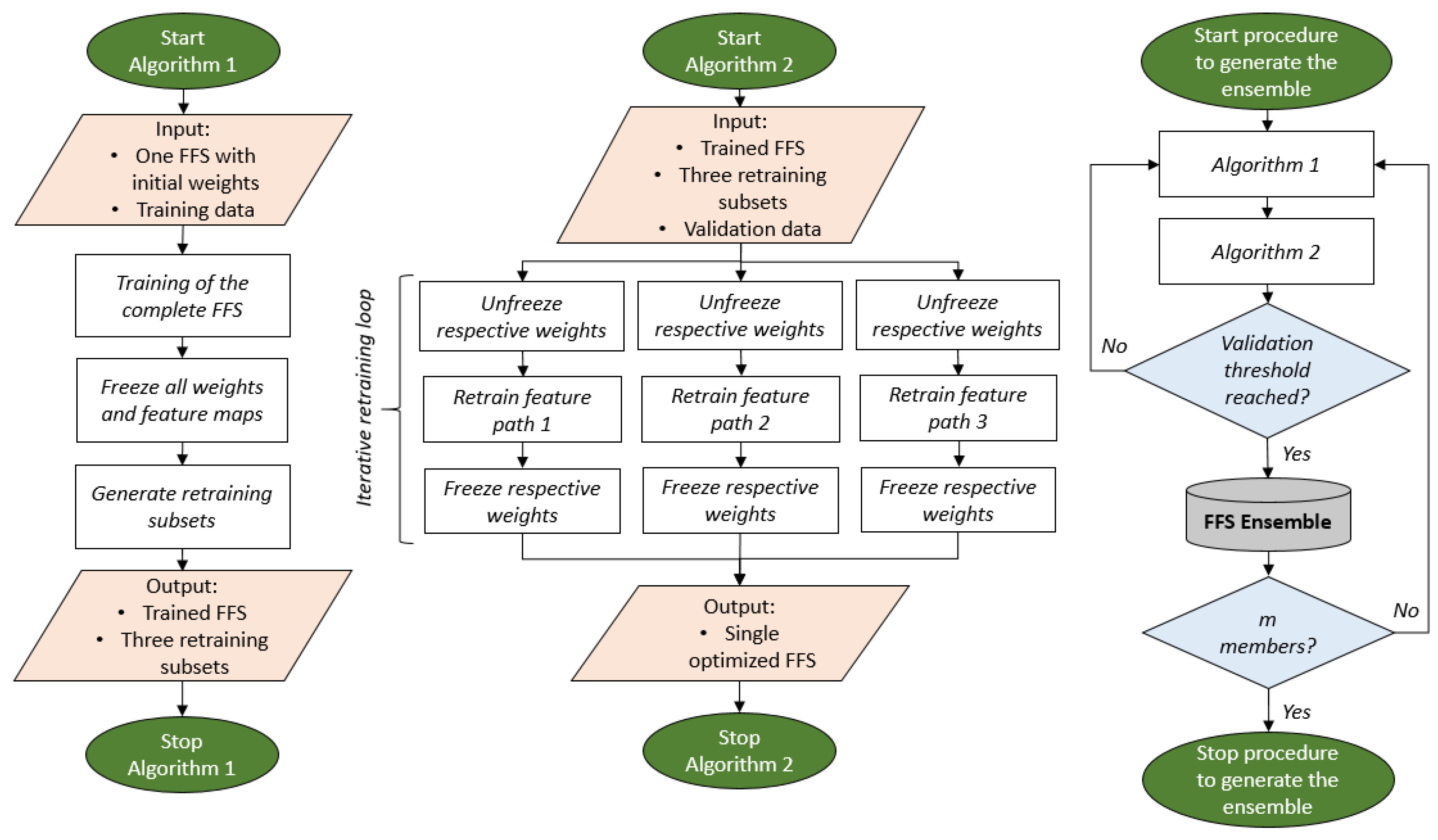
2.3. Optimization and Ensemble Approach

By adjusting the feature maps in the ResNet50 architecture and the weights and biases in the feature-informed part, the data-driven model can be trained to optimize its prediction. The objective is to find the water depth predictions that agree the most with the physically based inundation maps. The agreement and thus quality are defined by the loss function ( L F ).
We applied the mean squared error ( M S E ) as L F , where: P are the predicted values, T the observed values, and n is the number of predictions:
L F = M S E = 1 n i = 1 n ( P T ) 2
During the training procedure, a minimum value of this L F is searched by the optimization algorithm. We used Adams’ optimizer, which is typically used and well-known [25].To ensure an optimal prediction/minimum error, we developed a novel workflow for the training procedure. The workflow is shown in Figure 3 and consists of 2 algorithms. In the first algorithm, the complete feature-informed data-driven model is trained on the training data. To set the focus of the prediction based on the features, after training we first freeze all weights and feature maps within the FFS, and then we generate three retraining subsets. Each subset includes the input discharge images (input) and the cells (true output) of each respective feature. After that, algorithm 1 is complete, providing as output a trained FFS and three retraining subsets.
Algorithm 2 uses the outputs of algorithm 1 and additionally the validation data as inputs. First, an iterative retraining loop around the three features is applied. As such the FFS is retrained separately for each feature path with the respective subset, while only the weights in the respective feature path are optimized. Therefore, only the weights of the corresponding feature path (either 1, 2, or 3) must be unfrozen in the path to be trained and have to be frozen again after training. This approach is necessary since algorithm 1 trains all features at once and therefore it is not possible to set a special focus on a single feature (and gain the optimal weights within this feature). Hence, to make sure the weights in each feature path are optimized to describe the flood depths and characteristics of the respective feature in the best possible way, this retraining strategy is applied. The output of algorithm 2 is then a single optimized FFS. This concludes algorithm 2.
It is common to use an ensemble approach for accounting for uncertainties in the forecast. Herein, and to provide multiple equally likely members (m) within the ensemble, the steps tasks of algorithms 1 and 2 are repeated. With this procedure, the final water depth for each cell to be predicted is given by the average value calculated by the members of the ensemble. This procedure makes it possible to capture the uncertainty caused by the random weight initialization at the start of the training [9,26]. A similar approach is used by Berkhahn and Neuweiler (2019) [9] and by Schmid and Leandro (2023), to account for uncertainty [24].
To ensure equal probability among the members while maintaining high prediction quality, a member is accepted only if the prediction error on the validation data is less than five centimeters. This is quantified by the root mean squared error (RMSE) (see Equation (4) in Section 2.4), which takes the square root of the LF. The procedure is sequential and starts with algorithms 1 and 2. After, it checks if the single optimized FFS reaches the validation threshold (RMSE below 0.05 m). If that is not the case, the optimized FFS is dismissed and algorithms 1 and 2 are repeated. If the validation threshold is reached, an ensemble member is accepted. A final condition checks whether the ensemble already consists of (at least) the desired members. The procedure is stopped if this condition is met. Otherwise, algorithms 1 and 2 are repeated. The model was trained on an NVIDIA Quadro M4000 graphics card with a memory of 8 GB. Such a card (or similar) is found commonly in many PCs. Python 3.9 and Tensorflow 2.6 were used for the development of the FFS.

2.4. Model Evaluation Criteria

To assess the performance of the FFS, two criteria are used, namely the mean squared error (MSE) (Equation (3)) and the root mean squared error (RMSE) (Equation (4)). The MSE is used to compare and validate the innovative methodology with the results obtained by Lin et al., 2020 [11]. The RMSE is used because the results are more intuitive to interpret as the error value has the same units as the water level. The observed values are taken as the results from the 2D hydrodynamic model HEC-RAS. The evaluation criteria are calculated for each event and each cell in the study area, resulting in a map representing the spatial distribution of the prediction error. Additionally, the average value is calculated, by dividing the RMSE by the number of cells to be predicted, to obtain a value for the entire study area.
R M S E = 1 n i = 1 n ( P T ) 2
where: P is the by the forecast system predicted value, T is the observed value, n is the number of predictions.

2.5. Study Site

The study area, Kulmbach (Figure 4), is located in Bavaria, Germany. The area has a size of about 12 km2 and nearly 27,000 people live in the area. The town center is located in the middle of the area. Three main rivers flow through the study area, namely the Schorgast, the Weißer Main, and the Roter Main. The flow direction is from northeast to southwest, where the area is narrow and surrounded by hills in the northeast. In the eastern part, the study site turns wider into a river floodplain.
As described in Section 2.2, the feature of the network is represented by the distance to the river lines. Therefore, for each cell to be forecasted, a GIS analysis was performed to calculate the distances to the rivers. The resulting distances were then classified into the three classes. Figure 5 shows this classification. Subsequently, the classes and respective cells were assigned to the three different paths within the network. The number of outputs within the last dense layers matches the number of cells of each class.

2.6. Dataset for Training, Validation, and Testing the Forecast System

A hybrid database containing 270 different events with their associated discharges and corresponding inundation maps is used to develop and test the FFS. The database was generated by Crotti et al. [6]. The authors have used a two-step procedure in which, first, the discharges for the three main rivers are generated by applying the hydrological model LARSIM (Large Area Runoff Simulation Model) [20], and second, the generated discharges are simulated with the hydrodynamic model HEC-RAS 2D [21] to obtain the corresponding maximum water levels in the catchment area as a map. The validation of the inundation model was performed by Bhola et al. in 2018 [27]. The hydrographs have an hourly resolution and 50 timesteps. To shape these hydrographs into the input tensor of 14 × 14 × 3, the 50 timesteps are extrapolated to fit into this frame. The maps are projected to a spatial resolution of 4 × 4 m, resulting in approximately 500,000 cells. One half (135 events) of the database consists of synthetic events produced by using return periods (durations: 5, 30, 90, 360, 720, and 1140 min and periods: 1, 50, 100, 200, 300, and 1000 years), and the other half (135 events) consists of real-based events. The real-based events are generated by scaling individual observed discharge events from time series analyses from 1970 to 2017 of the three rivers to higher return periods so that flooding occurred. The remaining two events are historically observed events from the years 2005 and 2013, which lead to major flooding within the study area. Figure 6 shows these hydrographs.
The database (excluding the historical events) is randomly split into the three subsets training (70%), validation (15%), and testing (15%). The two observed historical events are used to test the FFS on real observed data. For further details on generating the hybrid database please refer to Crotti et al. [6]. We like to state the main focus of the study is the development of a data-driven approach. The validation and setup of the flood inundation model was carried out by Bhola et al., 2018 [27]. Hence grid size, hydrodynamic parameters, rainfall duration, and intensity were already given. Our methodology is in any case flexible and can be applied to any database or flood model in which parameters and rainfall events of interest may differ.

3. Results

3.1. Training Durations and Validation Accuracy

The application of the developed optimizing workflow (Figure 3) on the feature-informed architecture resulted in a candidate for the ensemble. Validation was based on a set of 40 random events from the hybrid database and as described in Section 2.3 we applied an ensemble strategy to consider uncertainty. In case the output of algorithm 2 reaches the validation threshold of 0.05 m, the candidate is added as a member of the ensemble. We set the number of members to three (m = 3). In our study, the workflow (Figure 3) was repeated 17 times until the final ensemble was reached. Table 1 shows the results of the first three integrated ensemble members and the best four candidates overall as well as the respective training times.

3.2. Performance of the Feature-Informed Forecast System

3.2.1. Overall Performance

To evaluate the overall performance of the developed FFS, the average RMSE values are calculated. Table 2 shows the results of the FFS on the test dataset and the two observed events. The FFS delivers very good results, achieving the aim of a high prediction quality. For the 35 test events, the FFS makes an average prediction error of only 5 cm for each cell in the entire study area. The results of the observed events also show a good and sufficient prediction quality, as they are under 10 cm and 15 cm errors, respectively.
Besides the high prediction performance, the FFS delivers these predictions within 19 s (the pure prediction of a member is 3 s).

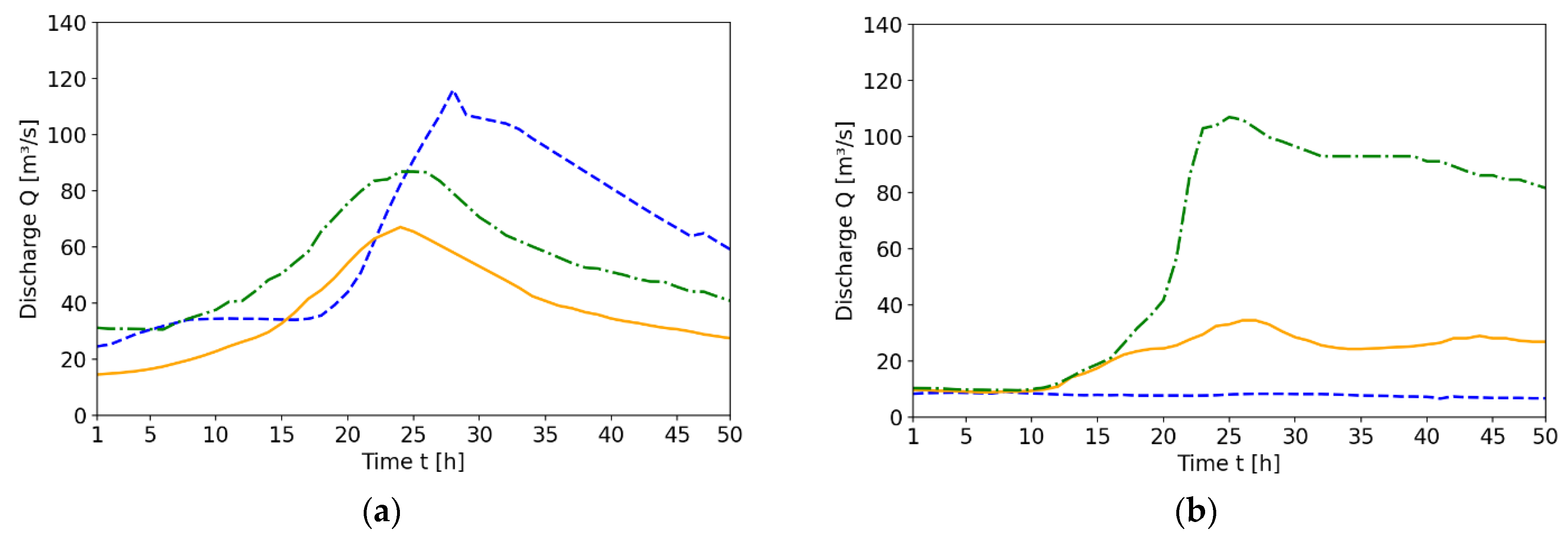
3.2.2. Comparison of the Individual Feature Performance on the Observed Events

We investigate the performance of the individual features on the observed events. Table 3 summarizes these results. It can be detected feature 2 performs nearly exactly like the overall average RMSE, whereas feature 1 shows around 40% better, and feature 3 40% worse results than the overall average prediction RMSE.

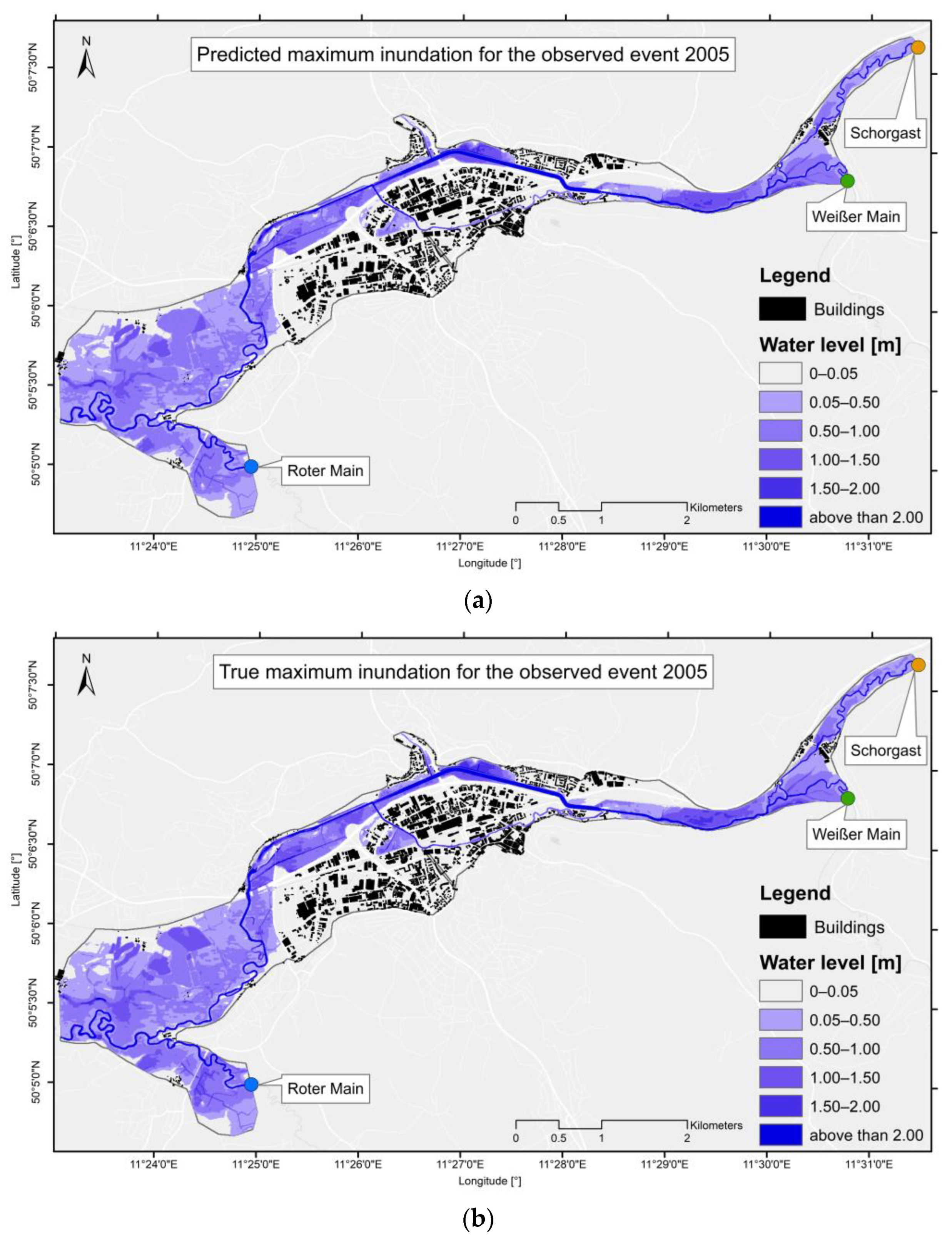
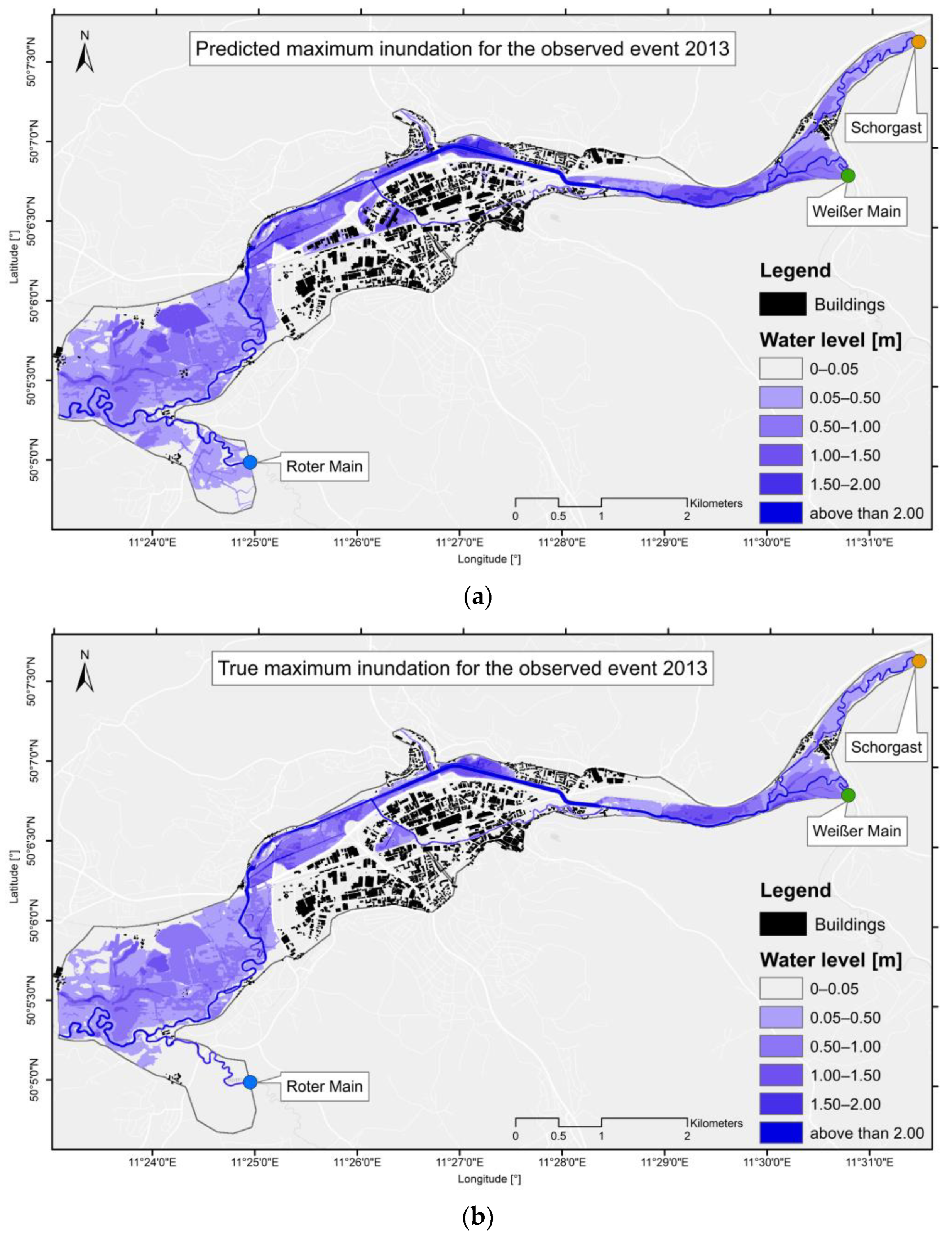
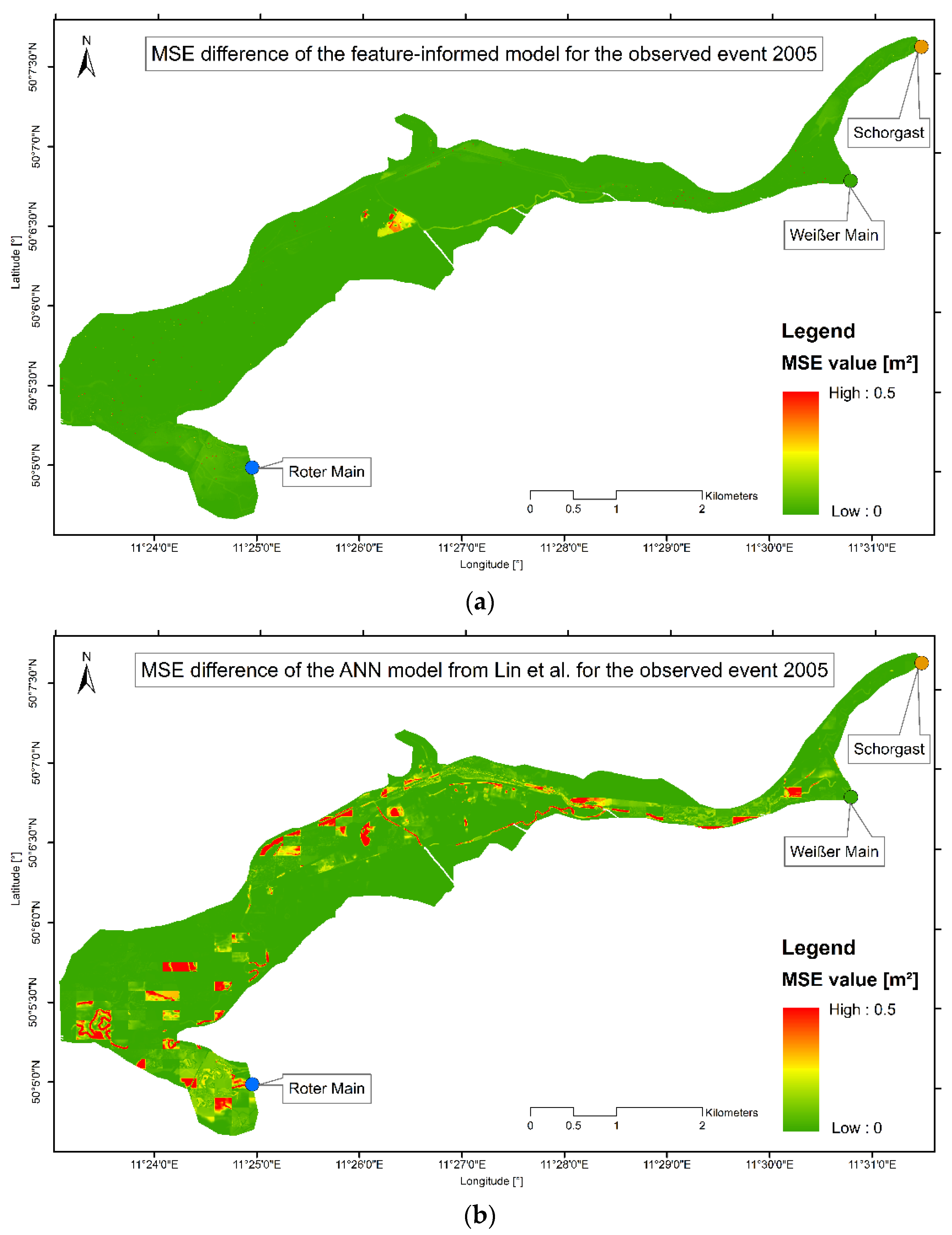
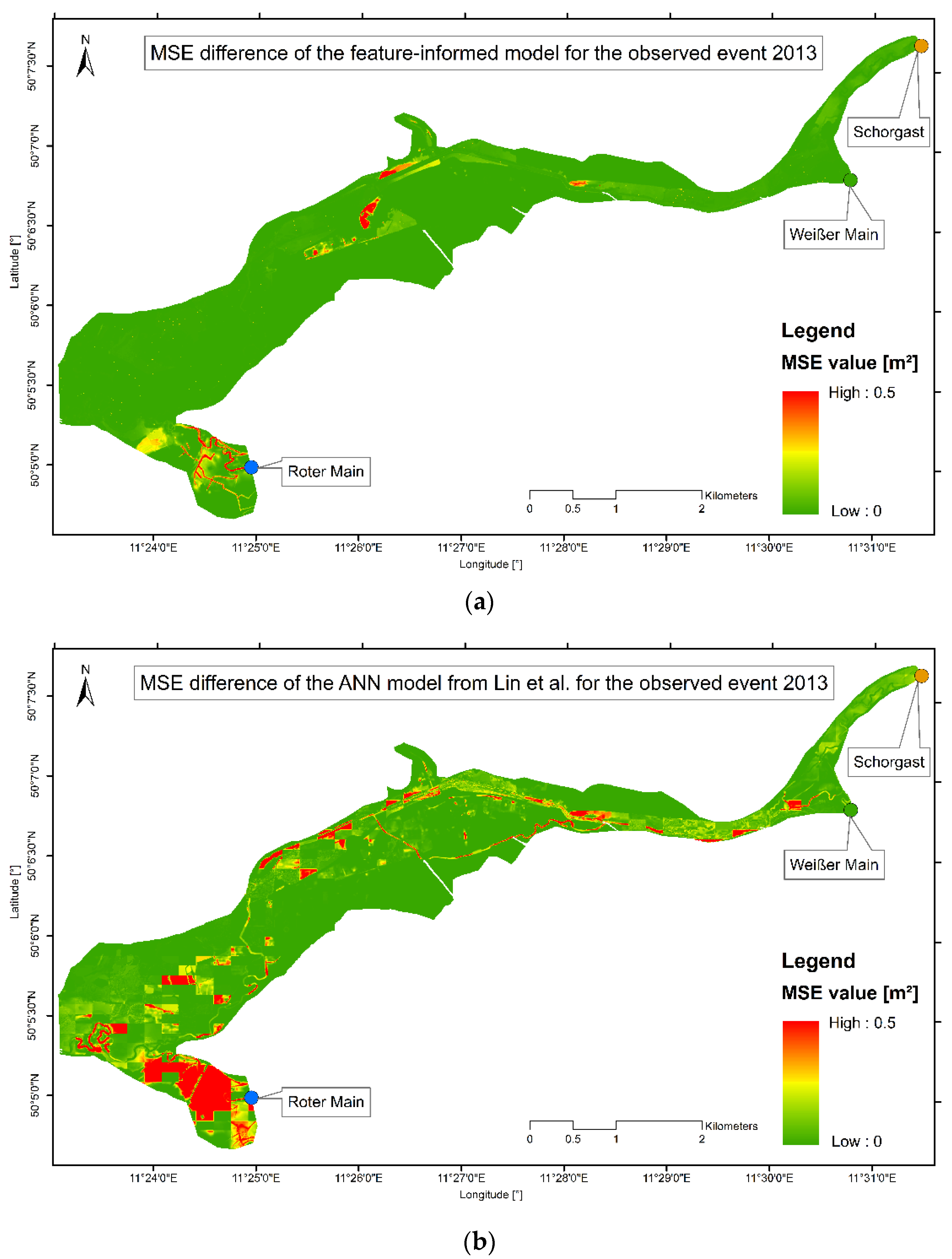
3.2.3. Inundation Maps and Spatially Distributed Prediction Error of the Observed Events

The inundation maps of the observed events from the years 2005 and 2013 are presented in Figure 7a and Figure 8a. Additionally, the respective true inundation gained by the HEC-RAS 2D model is visualized (Figure 7b and Figure 8b). It is clearly visible both maps (predicted and true) are very similar.
To further investigate the performance of the observed events, the MSE value is calculated for each cell to visualize the spatial prediction error. Since Lin et al., 2020 also developed a data-driven approach following multiple ANNs for predicting the inundation in the same study area, we can compare the results of their MSE maps with ours [11]. Figure 9 and Figure 10 visualize this comparison. It is seen our feature-informed architecture produces better predictions.

4. Discussion

4.1. Training Durations and Validation Accuracy

The results presented in Table 1 are very good. This is due to the newly developed optimization workflow. The iterative training process ensures every path is optimized separately and specialized to its respective feature. This procedure ensures the integration of additional knowledge (in our case the distance to the river) into the model. Furthermore, by following this approach there is no need to present the network with an additional GIS-layer dataset like [19], and on the other hand, there is no need to make compromises in the prediction quality since flood-influencing data are missing. This also allows training the model on a standard computer and predicting the entire study area using a single data-driven model. Besides that, the effective computational times for the training duration are attributed to the use of a ResNet50 in the classification part, as this is a convolutional network. This was responsible for the short training durations and thus made the optimization of the model more efficient. Therefore, it was possible to consider the uncertainty origin from the initial weights and integrate a threshold value for the validation, which in turn improved the prediction quality. The selection of a small number of the total members of the ensemble is done to ensure the time required for a single prediction is feasible on a standard computer and therefore is kept within a few seconds. Nevertheless, our workflow and methodology are also applicable to high-performance computing facilities for which the number of members does not impact the performance of the FFS.

4.2. Performance of the Feature-Informed Forecast System

4.2.1. Overall Performance

Table 2 shows the overall performance results of the FFS to the test dataset and the two observed events. These very good performances highlight the effectiveness of the image-to-image translation strategy of the feature-informed architecture (Figure 2) and the developed optimization workflow (Figure 3). The average RMSE values for our test data are better than those of Lin et al., 2020 (RMSE value of 0.316) [11]. The performances of the FFS for the observed events are of sufficient quality as well. The slightly worse performance for the event from 2013 can be explained by the lack of similar hydrograph shapes found in the training set. In the training set, all three rivers contribute to the flood volume (as well as rising or falling limbs), which is in contrast to the hydrograph shapes from the 2013 event (Figure 6b). In the latter, only the Schorgast rises rapidly and remains high throughout the forecast period. The integration of more events like this into the training set would enhance, therefore, the performance of the FFS also in this event. Besides the performance quality, the prediction time of 19 s makes the FFS suitable for real-time applications.

4.2.2. Comparison of the Individual Feature Performance on the Observed Events

Table 3 shows a 40% worse performance of feature 3. This can be explained since these are the cells the furthest away from the river (compare Figure 5). They are only inundated during relatively higher discharge events. The FFS could benefit from more scenarios being included in the training data set, for the relationship between inundation and discharges to be better captured. On the other hand, Table 3 shows a 40% better performance for feature 1, which represents the cells closest to the river with the highest inundation.
The overall and individual performance of each feature leads us to conclude splitting the cell into the distance from the river and providing this information feature-wise to the data-driven model is a good strategy.

4.2.3. Inundation Maps and Spatially Distributed Prediction Error of the Observed Events

The predicted inundation maps for the observed events (Figure 7 and Figure 8) show only minimal differences compared to the true inundation. Small differences between predicted and true inundation can be found for the event from 2013 in the southwestern part of the study area (Figure 8). This issue can be attributed partly to the fact that the majority of these cells are in feature 3, which performs somewhat worse than the other two features (described in Section 4.2.2), and also to the fact that the training set does not contain similar hydrograph shapes to the 2013 event (see Section 2.6). Either expanding the training set or splitting the features further based on different categories (as described in Section 4.2.2) are possible strategies.
By evaluating the results and prediction error, cells with an error based on the MSE larger than 0.2 m2 were only 0.11% for the event in 2005. The comparison of the prediction error with the results achieved by Lin et al. in 2020, where the authors stated 8.97% of the cells have an MSE larger than 0.2 m2 [11], concluded therefore in a great prediction quality improvement. This can also be visually verified in Figure 9. The analysis of the observed event in 2013 concluded only 2.14% of the cells have an MSE larger than 0.2 m2. In comparison, Lin et al., 2020 achieved 13.62% [11]. This can once again be visually verified in Figure 10. This comparison demonstrates the effectiveness of our feature-informed data-driven approach.
Nevertheless, it should be also mentioned, besides the architecture and optimization workflow, the use of a hybrid database ensures this high prediction quality, especially on the observed events. Schmid and Leandro also found this to be true when they developed a prediction system based only on synthetic events [24].

4.3. Limitations and Future Research

It should be mentioned, for running the FFS three hydrographs are necessary and are given in this study. For real-time applications, this hydrograph has to be predicted beforehand. For this, there are multiple strategies for delivering a flood hydrograph in real time [28,29]. The FFS is trained based on the hydrodynamic model HEC-RAS 2D. Thus, structural and parameter uncertainties arising from using this model are included in the FFS. In any case, physically based models like HEC-RAS 2D are considered state-of-the-art for generating spatially distributed water depths and inundation maps and therefore the best choice for training [7].
As for the features, we integrated only the distance to the river for the sake of testing and demonstrating our methodology. However, there are more flood-influencing factors, like elevation, land use, or slope. Future studies could investigate the integration of more features into the forecast system. Besides that, in our approach, since we focused on the maximum water depth, we neglected the temporal resolution of the inundation. Future research should focus on providing a temporal multi-step forecast of the inundation in the study area.

5. Conclusions

This study presented the development of a forecast system to predict the maximum inundation for flood hydrographs. The FFS consists of a feature-informed data-driven model, which interprets the forecasting process as an image-to-image translation and combines a convolutional classification architecture (ResNet 50) with three paths of informed dense layers to generate the inundation map. The dense layers are informed by the distance of the respective cell to be predicted to a river. Based on our results, the following conclusions can be drawn.
  • The FFS delivers the prediction within 19 s, thus making the system usable for real-time applications.
  • The innovative training workflow with pre-simulated inundation scenarios from a hybrid database ensures a high prediction quality. The accuracy of the FFS compared with the physically based model HEC-RAS shows average RMSE values of 0.052 for 35 test events. A test on two observed flood events showed RMSE values of 0.074 and 0.141.
  • The feature-informed architecture makes it possible to integrate additional knowledge about flooding into the model without providing an additional dataset. This not only enhances the prediction performance, since it also allows training on a standard computer, making such an application accessible to a wider range of users. The prediction performance on two observed test events showed only 0.11% and 2.14% of the cells forecasted have an MSE value larger than 0.2 m2, an improvement as compared to the work of Lin et al., 2020 [11] which reached values of 8.97% and 13.62%.

Author Contributions

Conceptualization, F.S.; methodology, F.S.; software, F.S; validation, F.S; data curation, F.S.; writing—original draft preparation, F.S.; writing—review and editing, J.L.; visualization, F.S.; supervision, J.L. All authors have read and agreed to the published version of the manuscript.

Funding

The research presented in this paper has been carried out as part of the HiOS project (Hinweiskarte Oberflächenabfluss und Sturzflut) funded by the Bayerisches Staatsministerium für Umwelt und Verbraucherschutz (StMUV) [Bavarian State Ministry of the Environment and Consumer Protection] (69-0270-92086/2017) and supervised by the Bayerisches Landesamt für Umwelt (LfU) [Bavarian Environment Agency].

Data Availability Statement

The datasets generated for this study are available upon request to the corresponding author.

Acknowledgments

We would like to thank Qing Lin (Justus Liebig University Gießen—Center for International Development and Environmental Research (ZEU)) for sharing the data from his article: Prediction of Maximum Flood Inundation Extents With Resilient Backpropagation Neural Network: Case Study of Kulmbach.

Conflicts of Interest

The authors declare no conflict of interest.

References

  1. Swiss RE Institue Sigma—Natural Catastrophes in 2021: The Floodgates Are Open. Available online: https://www.swissre.com/institute/research/sigma-research/sigma-2022-01.html (accessed on 11 December 2023).
  2. Arnell, N.W.; Lloyd-Hughes, B. The Global-Scale Impacts of Climate Change on Water Resources and Flooding under New Climate and Socio-Economic Scenarios. Clim. Chang. 2014, 122, 127–140. [Google Scholar] [CrossRef]
  3. Bevacqua, E.; Maraun, D.; Vousdoukas, M.I.; Voukouvalas, E.; Vrac, M.; Mentaschi, L.; Widmann, M. Higher Probability of Compound Flooding from Precipitation and Storm Surge in Europe under Anthropogenic Climate Change. Sci. Adv. 2019, 5, eaaw5531. [Google Scholar] [CrossRef] [PubMed]
  4. Calvin, K.; Dasgupta, D.; Krinner, G.; Mukherji, A.; Thorne, P.W.; Trisos, C.; Romero, J.; Aldunce, P.; Barrett, K.; Blanco, G.; et al. IPCC, 2023: Climate Change 2023: Synthesis Report. Contribution of Working Groups I, II and III to the Sixth Assessment Report of the Intergovernmental Panel on Climate Change; Core Writing Team, Lee, H., Romero, J., Eds.; IPCC: Geneva, Switzerland, 2023. [Google Scholar]
  5. Rözer, V.; Peche, A.; Berkhahn, S.; Feng, Y.; Fuchs, L.; Graf, T.; Haberlandt, U.; Kreibich, H.; Sämann, R.; Sester, M.; et al. Impact-Based Forecasting for Pluvial Floods. Earth’s Future 2021, 9, 2020EF001851. [Google Scholar] [CrossRef]
  6. Crotti, G.; Leandro, J.; Bhola, P.K. A 2D Real-Time Flood Forecast Framework Based on a Hybrid Historical and Synthetic Runoff Database. Water 2019, 12, 114. [Google Scholar] [CrossRef]
  7. Henonin, J.; Russo, B.; Mark, O.; Gourbesville, P. Real-Time Urban Flood Forecasting and Modelling—A State of the Art. J. Hydroinform. 2013, 15, 717–736. [Google Scholar] [CrossRef]
  8. Sun, W.; Bocchini, P.; Davison, B.D. Applications of Artificial Intelligence for Disaster Management. Nat. Hazards 2020, 103, 2631–2689. [Google Scholar] [CrossRef]
  9. Berkhahn, S. An Ensemble Neural Network Model for Real-Time Prediction of Urban Floods. J. Hydrol. 2019, 12, 743–754. [Google Scholar] [CrossRef]
  10. Kimura, N.; Yoshinaga, I.; Sekijima, K.; Azechi, I.; Baba, D. Convolutional Neural Network Coupled with a Transfer-Learning Approach for Time-Series Flood Predictions. Water 2019, 12, 96. [Google Scholar] [CrossRef]
  11. Lin, Q.; Leandro, J.; Wu, W.; Bhola, P.; Disse, M. Prediction of Maximum Flood Inundation Extents With Resilient Backpropagation Neural Network: Case Study of Kulmbach. Front. Earth Sci. 2020, 8, 332. [Google Scholar] [CrossRef]
  12. Kabir, S.; Patidar, S.; Xia, X.; Liang, Q.; Neal, J.; Pender, G. A Deep Convolutional Neural Network Model for Rapid Prediction of Fluvial Flood Inundation. J. Hydrol. 2020, 590, 125481. [Google Scholar] [CrossRef]
  13. Guo, Z.; Leitão, J.P.; Simões, N.E.; Moosavi, V. Data-driven Flood Emulation: Speeding up Urban Flood Predictions by Deep Convolutional Neural Networks. J. Flood Risk Manag. 2021, 14, e12684. [Google Scholar] [CrossRef]
  14. Hofmann, J.; Schüttrumpf, H. floodGAN: Using Deep Adversarial Learning to Predict Pluvial Flooding in Real Time. Water 2021, 13, 2255. [Google Scholar] [CrossRef]
  15. Burrichter, B.; Hofmann, J.; Koltermann da Silva, J.; Niemann, A.; Quirmbach, M. A Spatiotemporal Deep Learning Approach for Urban Pluvial Flood Forecasting with Multi-Source Data. Water 2023, 15, 1760. [Google Scholar] [CrossRef]
  16. Russell, S.J.; Norvig, P.; Chang, M.; Devlin, J.; Dragan, A.; Forsyth, D.; Goodfellow, I.; Malik, J.; Mansinghka, V.; Pearl, J.; et al. Artificial Intelligence: A Modern Approach, 4th ed.; Pearson Series in Artificial Intelligence; Pearson: Harlow, UK, 2022; ISBN 978-1-292-40113-3. [Google Scholar]
  17. O’Shea, K.; Nash, R. An Introduction to Convolutional Neural Networks. arXiv 2015, arXiv:1511.08458. [Google Scholar]
  18. Li, Z.; Liu, F.; Yang, W.; Peng, S.; Zhou, J. A Survey of Convolutional Neural Networks: Analysis, Applications, and Prospects. IEEE Trans. Neural Netw. Learn. Syst. 2022, 33, 6999–7019. [Google Scholar] [CrossRef]
  19. Löwe, R.; Böhm, J.; Getreuer Jensen, D.; Leandro, J.; Højmark Rasmussen, S. U-FLOOD—Topographic Deep Learning for Predicting Urban Pluvial Flood Water Depth. J. Hydrol. 2021, 603, 126898. [Google Scholar] [CrossRef]
  20. Ludwig, K.; Bremicker, M. The Water Balance Model LARSIM—Design, Content and Applications; Freiburger Schriften zur Hydrologie: Freiburg, Germany, 2006; Volume 22. [Google Scholar]
  21. US Army Corps of Engineers, Hydrologic Engineering Center. HEC-RAS River Analysis System—2D Modeling Users Manual 2016. Available online: https://www.hec.usace.army.mil/software/hec-ras/documentation/HEC-RAS%205.0%202D%20Modeling%20Users%20Manual.pdf (accessed on 11 December 2023).
  22. He, K.; Zhang, X.; Ren, S.; Sun, J. Deep Residual Learning for Image Recognition. arXiv 2015, arXiv:1512.03385. [Google Scholar]
  23. Chiang, Y.-M.; Chang, L.-C.; Tsai, M.-J.; Wang, Y.-F.; Chang, F.-J. Dynamic Neural Networks for Real-Time Water Level Predictions of Sewerage Systems-Covering Gauged and Ungauged Sites. Hydrol. Earth Syst. Sci. 2010, 11, 1309–1319. [Google Scholar] [CrossRef]
  24. Schmid, F.; Leandro, J. An Ensemble Data-Driven Approach for Incorporating Uncertainty in the Forecasting of Stormwater Sewer Surcharge. Urban Water J. 2023, 20, 1140–1156. [Google Scholar] [CrossRef]
  25. Kingma, D.P.; Ba, J. Adam: A Method for Stochastic Optimization. arXiv 2017, arXiv:1412.6980. [Google Scholar]
  26. Blundell, C.; Cornebise, J.; Kavukcuoglu, K.; Wierstra, D. Weight Uncertainty in Neural Networks. arXiv 2015, arXiv:1505.05424. [Google Scholar]
  27. Bhola, P.; Leandro, J.; Disse, M. Framework for Offline Flood Inundation Forecasts for Two-Dimensional Hydrodynamic Models. Geosciences 2018, 8, 346. [Google Scholar] [CrossRef]
  28. Tayfur, G.; Singh, V.; Moramarco, T.; Barbetta, S. Flood Hydrograph Prediction Using Machine Learning Methods. Water 2018, 10, 968. [Google Scholar] [CrossRef]
  29. Tayfur, G. Real-Time Flood Hydrograph Predictions Using Rating Curve and Soft Computing Methods (GA, ANN). In Handbook of Hydroinformatics; Elsevier: Amsterdam, The Netherlands, 2023; pp. 325–338. ISBN 978-0-12-821962-1. [Google Scholar]
Figure 1. The framework of the forecast system (FS). The numbers on the right side refer to the explanation in the numbered list below.
Geosciences 13 00384 g001
Figure 2. The architecture of the feature-informed data-driven model.
Geosciences 13 00384 g002
Figure 3. Workflow for the optimization and the generation of the ensemble with m members.
Geosciences 13 00384 g003
Figure 4. The study site: Kulmbach. The subplot in the upper left shows the location of Kulmbach within Germany.
Geosciences 13 00384 g004
Figure 5. Visual representation of the integrated feature: distance to the rivers.
Geosciences 13 00384 g005
Figure 6. Observed hydrographs time series. Orange (continuous) represents the Schorgast, green (dashed-dotted) the Weißer Main, and blue (dotted) the Roter Main: (a) hydrograph from the year 2005; (b) hydrograph from the year 2013.
Geosciences 13 00384 g006
Figure 7. Inundation maps for the observed flood event from 2005. The input hydrographs are shown in Figure 6a: (a) prediction of the feature-informed forecast system; (b) true inundation delivered by the physically based model HEC-RAS 2D.
Geosciences 13 00384 g007
Figure 8. Inundation maps for the observed flood event from 2013. The input hydrographs are shown in Figure 6b: (a) prediction of the feature-informed forecast system; (b) true inundation delivered by the physically based model HEC-RAS 2D.
Geosciences 13 00384 g008
Figure 9. MSE comparison of the ANN approach from Lin et al., 2020 [11] and our feature-informed approach. The MSE is calculated by the difference between the neural approach and the hydrodynamic model of the observed event in 2005: (a) MSE difference of the feature-informed forecast system; (b) MSE difference of the ANN approach from Lin et al., 2020 [11].
Geosciences 13 00384 g009
Figure 10. MSE comparison of the ANN approach from Lin et al., 2020 [11] and our feature-informed approach. The MSE is calculated by the difference between the neural approach and the hydrodynamic model of the observed event in 2013: (a) MSE difference of the feature-informed forecast system; (b) MSE difference of the ANN approach from Lin et al., 2020 [11].
Geosciences 13 00384 g010
Table 1. Training time and validation accuracy for the feature-informed forecast data-driven model, for the top four procedures. Only the first three are selected for the ensemble. Procedure 4 is the first to go over the selection threshold.
Validation Accuracy [RMSE]Training Time [min]
Output of algorithm 2: 1 0.039 m126
Output of algorithm 2: 2 0.042 m131
Output of algorithm 2: 3 0.048 m116
Output of algorithm 2: 4 0.051 m125
Table 2. The average accuracy of the forecast system on the test dataset and the observed events.
Accuracy [RMSE]
Test dataset (35 events)0.052 m
Observed event 20050.074 m
Observed event 20130.141 m
Table 3. Comparison of the average MSE performance of the individual feature.
RMSE of Feat. 1RMSE of Feat. 2RMSE of Feat. 3
(Cells Up to 150 m Away)(Cells Up to 400 m Away)(Cells > 400 m Away)
Observed event 20050.063 m0.070 m0.078 m
Observed event 2013 0.101 m0.141 m0.152 m
Disclaimer/Publisher’s Note: The statements, opinions and data contained in all publications are solely those of the individual author(s) and contributor(s) and not of MDPI and/or the editor(s). MDPI and/or the editor(s) disclaim responsibility for any injury to people or property resulting from any ideas, methods, instructions or products referred to in the content.

