Quantifying Drought Characteristics in Complex Climate and Scarce Data Regions of Afghanistan

Abstract

Droughts cause critical and major risk to ecosystems, agriculture, and social life. While attempts have been made globally to understand drought characteristics, data scarcity in developing countries often challenges detailed analysis, including climatic, environmental, and social aspects. Therefore, this study developed a framework to investigate regional drought analysis (RDA) using regional drought intensity-duration-frequency (RD-IDF) curves and regional drought risk assessment (RDRA) based on the drought hazard indicator (DHI) and drought vulnerability indicator (DVI) for scarce data regions in Afghanistan. The drought characteristics were analyzed using the regional standardized-precipitation-index (SPI), and standardized precipitation-deficit distribution (SPDD). Further, L-moment statistics were used to classify different homogenous regions based on regional frequency analysis (RFA). The historical monthly precipitation data from 23 rainfall stations for the years 1970 to 2016 were collected from the Ministry of Water and Energy of Afghanistan. Based on the analysis performed, the area was classified into six homogeneous regions R-1, R-2, R-3, R-4, R-5, and R-6. The drought was very consistent—almost 50% of the years—irrespective of the homogeneous region classified. R-4, located in the northeast of the country, had a one-year extreme drought with high resiliency and low risk to drought compared to other regions. As R-1, R-3 and R-5 are located in the southwest, center and southeast parts of Afghanistan, they experience moderate drought with low resiliency and high drought risk due to long period of droughts. Moreover, the uniform distribution of precipitation deficit (D_m), was less in arid climate regions. In contrast, the semi-arid climate regions showed higher values of D_m. Furthermore, in the results in all the regions, the IDF curves showed a high drought intensity with increasing drought return periods. In contrast, the intensity significantly decreased when the time scale increased, and fewer were enhanced within the increasing drought return period. However, the outcome of this study may contain essential information for end users to make spatially advanced planning for drought effect mitigation in Afghanistan.

1. Introduction

Droughts are widespread natural disasters, exacerbated by climate change and severely affecting ecosystems, agriculture, food security, and social life in many parts of the world [1,2]. In Asia, rising temperature and altered precipitation patterns have led to water scarcity in many regions [3,4], and Afghanistan is the 12th most vulnerable country to climate change, according to the Notre Dame Global Adaptation Index 2021 [5]. However, nearly 80 percent of the population in Afghanistan are heavily dependent on agriculture and livestock for a livelihood and are often affected by climate change [6]. Therefore, to address this critical issue, a framework needs to be developed that includes: a) regional drought analysis (RDA) for investigating the regional drought risk assessment (RDRA) and b) information tools in the form of regional drought intensity-duration-frequency (RD-IDF) curves for agro-climatic and hydro-climatic planning to develop drought mitigation measures. However, obtaining adequate data for regional drought analysis remains challenging, especially in the least developed countries like Afghanistan [7]. Probabilistic models are often preferred for drought analysis using point or multi-site data spanning several decades. However, limited data estimation by conventional techniques, such as the product–moment method, often results in unrealistic drought estimates [8]. Contrary to this, the L-moment method proved to be more efficient than conventional methods in estimating drought probabilities with limited data [7,9]. This approach allows regions with limited weather stations to achieve better consistency in frequency estimation and magnitude even in ungauged areas, by combining the conceptual statistics from several stations in the homogeneous region [9].

Limited studies in arid and semi-arid regions have used the L-moment method for regional drought probability studies. For instance, occurrence of severe drought in the arid and semi-arid region of Chile was estimated using regional frequency analysis (RFA) based on the mean annual precipitation (MAP) with the L-MAP software 2010 tool [8]. The drought frequency in Portugal was studied using the standardized precipitation index (SPI) on different time scales to characterize the drought events [10], and the spatial variation of annual maximum dry spell lengths were analyzed using the regional frequency distribution with L-moment statistics [11]. Similarly, L-moment statistics were employed to present the areal pattern of annual maximum dry spell length using RFA [6] and the occurrence of the severe drought events, along with the risk based on the different return periods [12]. Additionally, Zhang et al. [13] considered the joint probability behavior of droughts based on RFA and categorized the homogeneous regions using the multivariate L-moment method and the Fuzzy C- Means (FCM) clustering technique. Furthermore, Nunez et al. [14] proposed an integrated method for RFA-L-moment application under large-network-high-complex-spatial-scale-conditions. Finally, Kaluba et al. [7] assessed the spatial variation of meteorological droughts with their return periods in Zambia by developing the L-MAP using the mean annual precipitation MAP. These studies demonstrate the potential of the L-moment method in RDA for various hydro-climatic planning applications.

Prior to drought risk assessment (DRA), identifying the drought characteristics is essential. Several drought indices have been developed for the analysis of severity, duration, and frequency of drought. The commonly used indices include the Palmer drought severity index (PDSI) [15], crop moisture index (CMI) [16], standardized precipitation index (SPI) [17,18], soil moisture drought index (SMDI) [19], vegetation condition index (VCI) [20], standardized precipitation evapotranspiration index (SPEI) [21], and surface water supply index (SWSI) [22]. However, each of the above indices have different data requirements, limiting their applicability in data scarce under-developed or developing countries. In contrast, SPI is often preferred as it needs only precipitation data [17,18]. A detailed description of the SPI along with its advantages is available in a wide range of literature [17,18,23,24].

Drought risk assessment (DRA) is often based on drought hazard indicators (DHI) and drought vulnerability indicators (DVI). While the definitions of hazard and vulnerability differ across studies [25], vulnerability commonly assesses the impact of a natural hazard on a human population, and hazard represents the possibility of an adverse natural physical event [26]. Comprehensive DRA involves understanding the socio-physical interactions between humans and the natural environment, which necessitates the use of multiple social indicators [27,28]. However, only a few studies have explored DRA using DHI and DVI linked with social indicators [29,30].

Frequency analysis is commonly used in hydro-meteorological data analysis such as droughts. However, drought frequency alone is not sufficient to characterize the drought events. Understanding the duration, severity, and intensity (in the form of drought curves) of droughts is required [31]. The drought intensity-duration-frequency (D-IDF) curve is an important tool in drought analysis that investigates interrelationships between drought characteristics [32]. Among the limited studies, IDF curves developed using the precipitation deficit based on SPI to calculate the severity and intensity in the duration-frequency curves [32], and critical drought IDF curves using the standardized precipitation index [31] are important. Other notable studies include severity-duration-frequency (SDF) and severity area frequency (SAF) curves based on homogeneous drought regions using copulas [33], development of drought severity area frequency (SAF) curves to investigate the impact of climate change [34] and drought severity duration frequency (SDF) relationships of dry and wet periods using the palmer drought severity index (PDSI) [35].

2. Materials and Methods

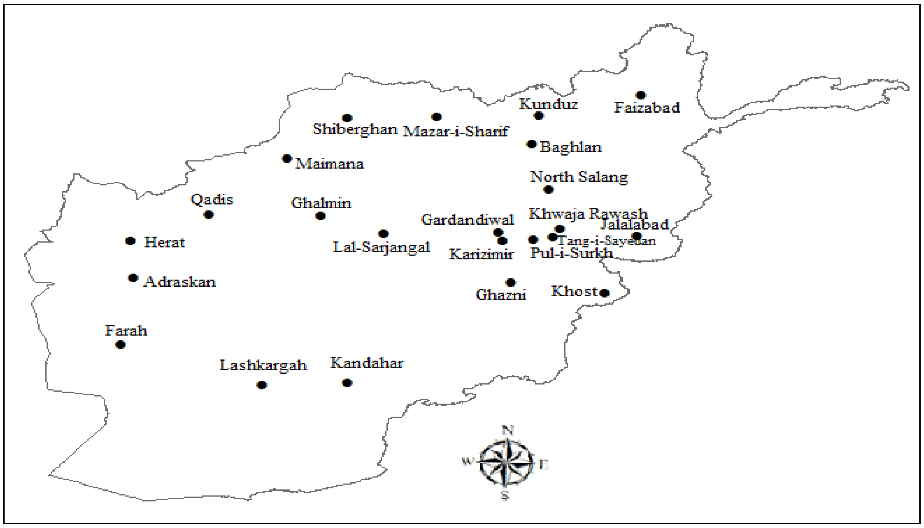
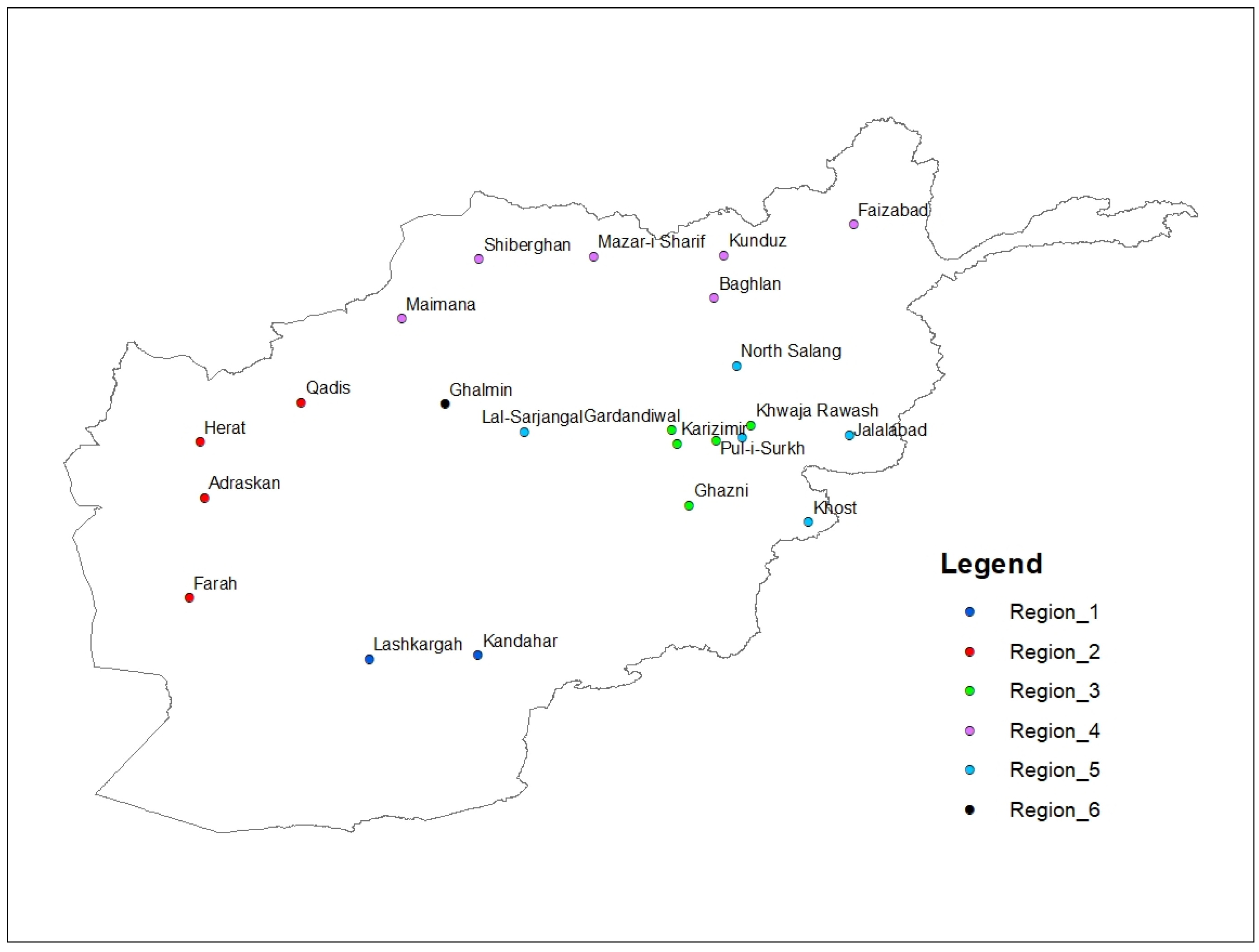
2.1. Study Area and Data Used

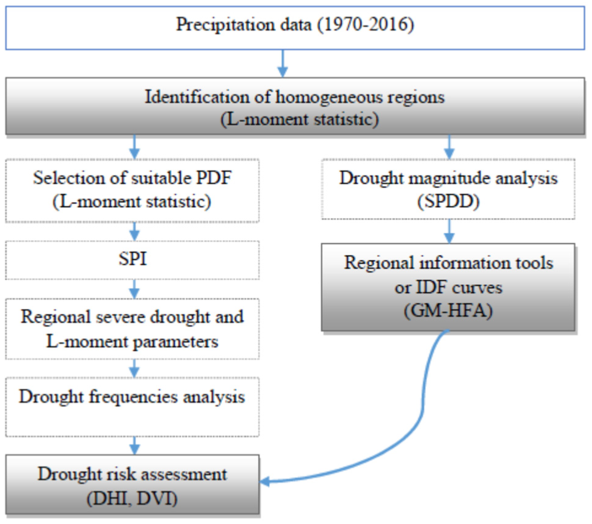
Afghanistan is located in the southwest of Central Asia (29° to 39° N; 60° to 75° E), with a population of 34 million, of which more than 70% live in rural areas. The total area of Afghanistan is about 652,000 km² and nearly 75 percent of the land is mountainous and desert terrain [36]. Parts of the mountainous area with altitudes above 2000 m (such as Hindu Kush, Wakhan, and Baba) are covered by snow, which is the source of around 80% of the country’s need. The snowmelt in the summer contributes significantly to the runoff in all the major river basins (such as Amu Darya, Harirud–Murghab, Helmand, Northern, and Kabul Indus). The total area available for cultivation is about 8 million hectares (12 percent of the total area); however, only around 3.9 million hectares are currently under cultivation of which 1.3 million ha is rainfed and 2.6 million ha is irrigated [37]. The country experiences diverse climates, ranging from subtropical and continental to cold and polar tundra. According to Köppen–Geiger climate classification, five climate zones are identified: (i) arid desert in the southwest, (ii) arid steppe in the northwest, (iii) temperate dry summer in the center, (iv) cold dry summer in the north and east, and (v) polar tundra in the southeast. Furthermore, altitude plays a major role in the variations in precipitation across these climate zones. The southern region is characterized by cold desert climate, while the southeast experiences relatively higher rainfall due to the influence of the Indian monsoon. The central, northeast, and east parts of the country are mountainous and receive snow during the winter that feeds almost all the river basins with snow melt during the summer. However, the northern and some parts of the central east areas have cold summers with semi-arid climates, while the northwest area has warm summers with semi-arid climates. Further, the southwest of the country has warm summers with an arid climate. The country also has a broad range of temperature variations. While the mean monthly temperature in the winter season ranges from 0 to 8 °C, the absolute minimum temperature recorded in the month of January ranges from −20 to −25 °C. During the summer season, the mean temperature ranges from 24 to 32 °C with an absolute maximum temperature of 45 °C in July [38].

The historical monthly precipitation data for 47 years (1970 to 2016) from 23 precipitation stations obtained from the Ministry of Water and Energy in Afghanistan were used to perform the analysis proposed in the paper. The stations are spread widely across the country as shown in Figure 1. The annual time series data was used to estimate SPI for analyzing the severity and frequency of drought. The monthly precipitation deficit of the dry years was used to investigate drought IDF relationships.

2.2. Methodology

This study developed a comprehensive framework to analyze regional drought characteristics based on the regional drought risk assessment (RDRA) and regional drought intensity duration frequency (RD-IDF) curves using L-moment statistics. Historical precipitation data was used to identify the homogeneous regions. The relationships between severe droughts at regional scale and L-moment parameters were investigated within the identified homogeneous regions. Subsequently, regional SPI were calculated to analyze the occurrence probability of mild, moderate, and severe drought. To evaluate RDRA, the study introduces a unique method, utilizing the drought hazard indicator (DHI) and the drought vulnerability indicator (DVI), considering the drought occurrence probability and available water demand method. This novel approach enables the investigation of drought magnitudes based on monthly standardized precipitation-deficit distribution (SPDD). Furthermore, the study analyses drought IDF curves using the general model of hydrologic-frequency-analysis (GM-HFA). The entire methodology of this study is illustrated as a flowchart in Figure 2.

2.2.1. Identification of Homogeneous Regions

The classification of homogeneous regions is the most important step in RFA as it impacts the accuracy and reliability of subsequent analysis. The process involves grouping the sites with similar frequency distributions based on L-moment parameters. The groups are then subdivided until the final set of acceptable homogeneous regions is obtained.

The L-moment statistic is a linear combination of order statistics and a dramatic development over conventional product-moment statistics to characterize the forms of the probability distribution and estimate distribution parameters. This method is suitably related to the conventional product moment, where the sample sizes are small. L-moment statistics can be used in calculating sample statistics of records at an individual site, testing for homogeneity and heterogeneity, conducting the goodness of fit test of the selected probability distribution, and also for solving the distribution parameters [9]. However, this study estimates the ratios of L-CV (τ₂), L-skewness (τ₃), and L-Kurtosis (τ₄) to classify the homogeneous regions [9].

For screening the data to categorize the homogeneous regions (related to their frequency), L-moment distribution parameters (τ₂, τ₃, τ₄) of all the stations are plotted in two-dimensional space graphs. The points that are closer in the graphs indicate frequency similarity among the stations. The regions are defined by selecting adjacent points as groups of similar frequency. Additionally, a discordancy measure (D_i) is used to identify the stations that deviate significantly from others. This measure quantifies the dissimilarity of a site from the average L-moment parameter value of a group, and is calculated as in [9]:

$$D_i=\frac{N{(u_i-\overline{u})}^T(u_i-\overline{u})}{3xA}$$

(1)

where, N is number of sites in the group, u_i is a vector that contains the τ₂, τ₃, and τ₄ values for site i, and $\overline{u}$ is the average value of u_i. A is the matrix of sums of squares and cross-products. Stations with D_i values greater than 1.64 are considered as discordant [9]. Further, the regions are tested to examine whether a proposed region is homogeneous or heterogeneous, based on a heterogeneity measure (H):

$$H=\frac{(V-{\mu }_V)}{{\sigma }_V}$$

(2)

where, V is the weighted standard deviation of the site sample L-CV, μ_v is the mean value, and σ_v is standard deviation of the computed site variation. Based on the H absolute value, the region is considered as acceptably homogeneous (H < 1), possibly heterogeneous (1 < H < 2) and heterogeneous (H > 2) [9]. This test ensures that the identified homogeneous regions are consistent and reliable for subsequent drought analysis.

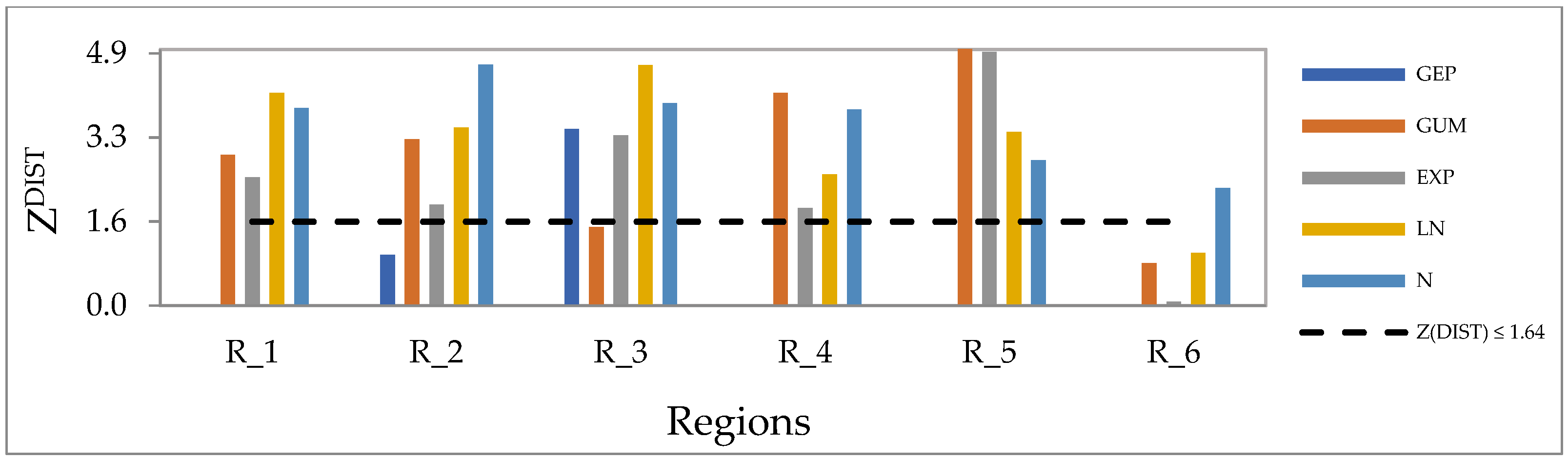
2.2.2. Selection of Suitable Probability Distribution Function (PDF)

In regional frequency analysis, data from multiple sites are combined to create a single region. As no single probability distribution perfectly fits the data from each site, it becomes imperative to identify appropriate distribution functions to suitably fit (i.e., best fit) the homogeneous regions [9,39]. To achieve this, five candidate distributions considered in this study are: (a) Generalized Pareto (GEP), (b) Gumbel (GUM), (c) Exponential (EXP), (d) Lognormal (LN), and (e) Normal (N) distributions for their suitability [7]. The best fit regional probability distribution is identified based on L-moment ratios [9]. The decision to select the best-fit regional frequency distribution is based on the Z^DIST, calculated as:

$$Z^{DIST}=\frac{({\tau }_4^R-{\tau }_4^{DIST})}{{\sigma }_4}$$

(3)

where, ${\tau }_4^R$ is the average of L-kurtosis calculated from the data of a region, τ₄^DIST and σ₄ are the average and standard deviation of L-kurtosis obtained for the fitted distribution, respectively. A good-fit distribution is selected when, Z^DIST ≤ 1.64. However, if more than one distribution meets this criterion, the distribution with the lowest Z^DIST value will be selected [9].

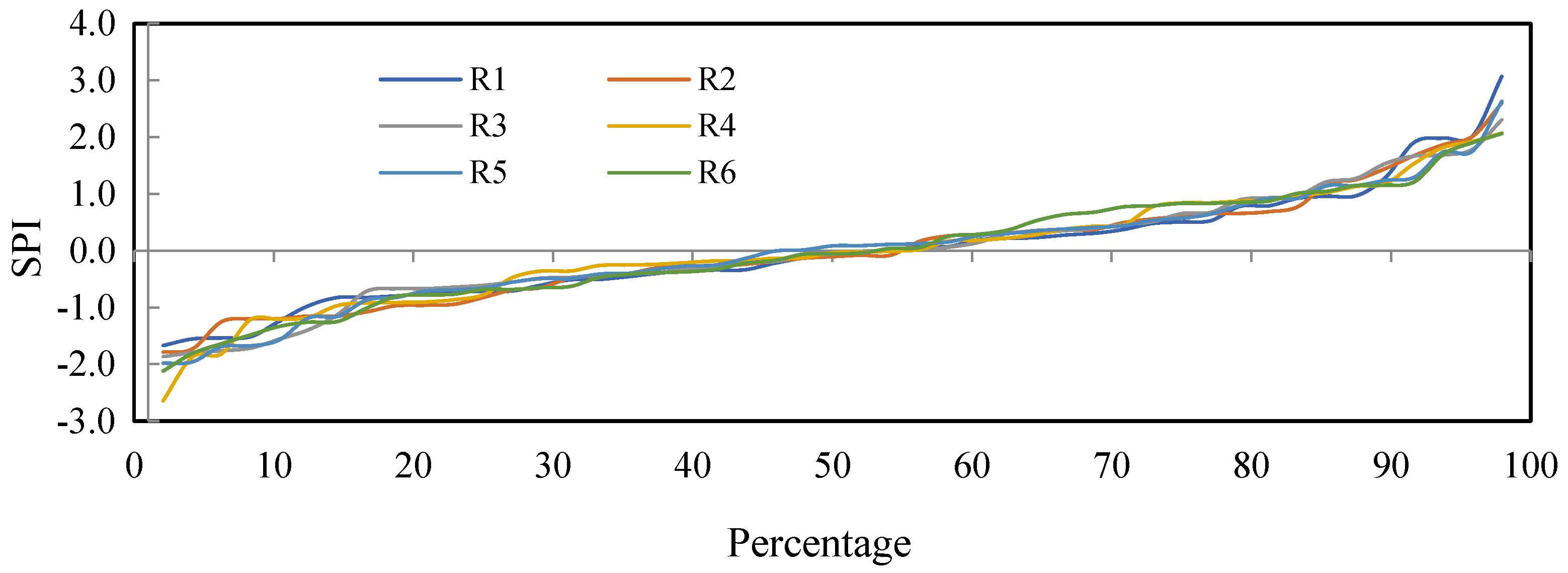
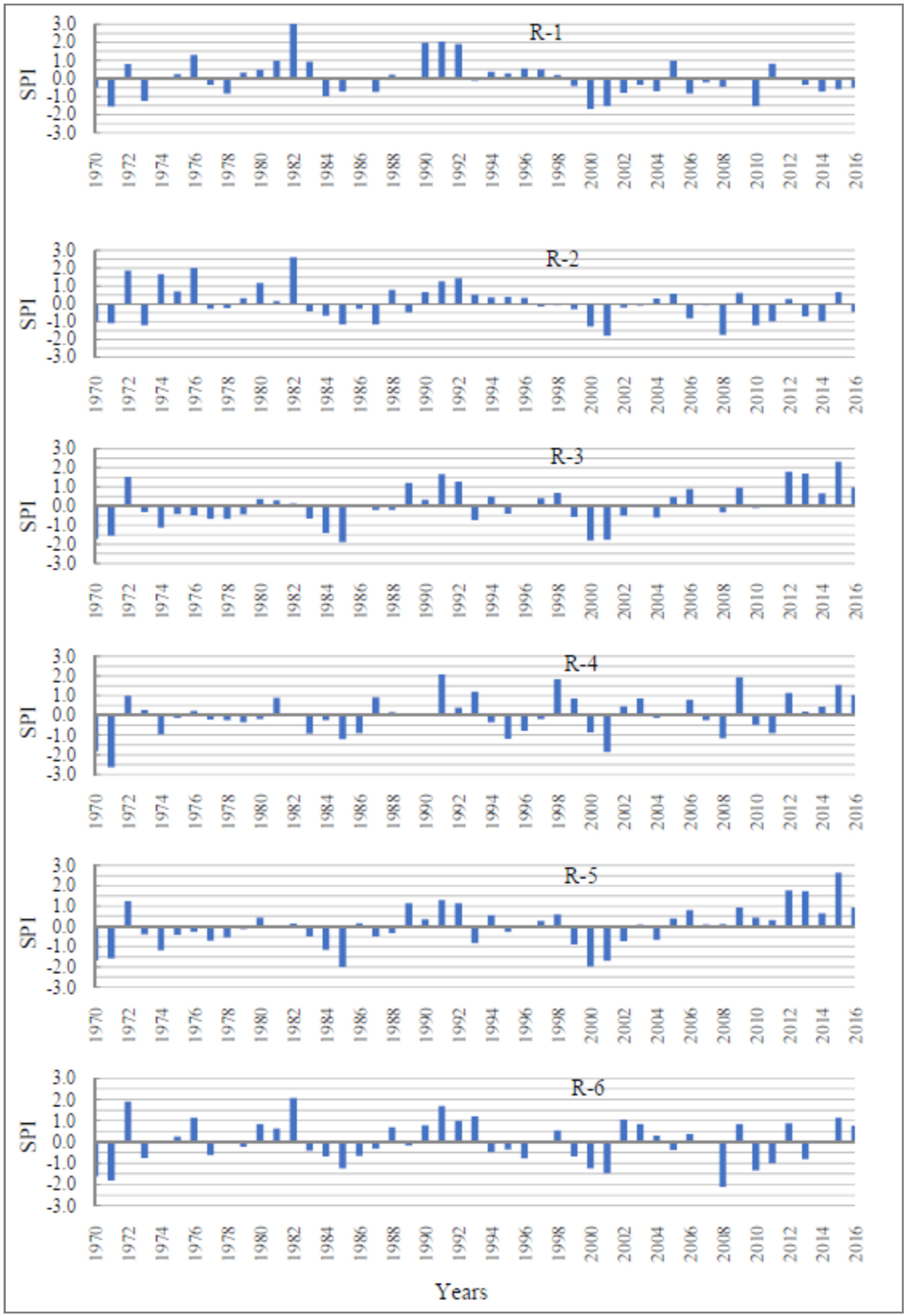
2.2.3. Standardized Precipitation Index (SPI)

The average precipitation data of the sites in the homogeneous regions are used to calculate the SPI for determining the drought severity [16]. The drought and wet years are classified based on the magnitude of the SPI value as shown in

Table 1. SPI Categories [40].

Categories	SPI Range
Extreme drought	SPI ≤ −2
Severe drought	−2 < SPI ≤ −1.5
Moderate drought	−1.5 < SPI ≤ −1
Mild drought	−1 < SPI < 0
Mild wet	0 ≤ SPI < 1
Moderate wet	1 ≤ SPI < 1.5
Severe wet	1.5 ≤ SPI < 2
Extreme wet	2 ≤ SPI

[40]. The most severe drought during all periods is identified by the minimum value of SPI [41]. During the dry period, the accumulated deficit of precipitation is referred to as the drought magnitude. Additionally, the total duration of all dry periods within a drought event is known as the drought duration.

2.2.4. Analysis of Relationships between Regional Severe Drought and L-Moment Parameters

The relationship between sub-regional values of the L-moments (L-CV and L-skewness) and MAP have been extensively studied to characterize the rainfall patterns, identify regional climate variability and occurrence of extreme weather events [7,8]. However, in this study we explored the above relationship using minimum SPI values from the homogeneous regions instead of MAP to analyze the relationships between regional drought events and L-moment ratios (L-Skewness). The modified exponential equation is formed as:

$$L-moment=\alpha \exp \left(-\beta \min SPI\right)+\delta$$

(4)

where, α, β and δ are fitting parameters obtained by analysis of least-squares optimization in the MS Excel Solver tool 2010.

2.2.5. Drought Frequency Analysis

The probability distribution of drought severity and duration is analyzed based on SPI values. The percentage of dry years within the data period is determined by plotting SPI values against the probability of time series. Additionally, drought severity is estimated through the SPI values of homogeneous regions which are arranged into descending order of magnitude. The probability distribution is prepared using the plotting-position [42].

Moreover, the study focuses on selecting drought and wet episodes from the regional SPI graphs. These episodes consist of one or more consecutive dry and wet years. In this section, we analyze the drought durations (in months) along with their return periods from the identified dry and wet episodes. The episodes are sorted in descending order, and we calculate the drought probability and return period for each spell (see Equation (5)).

$$\left.\begin{array}{c}\mathrm{SPI}=a\ln \left(T\right)+b\\ D=a\ln \left(T\right)+b\end{array}\right\}$$

(5)

2.2.6. Drought Risk Assessment

In the literature, various methods for risk assessment have been proposed with different definitions for risk. One such approach by Wisner et al. [43], views risk as a combination of vulnerability and hazard. In the context of drought, risk is commonly defined as the product of hazard and vulnerability [26,44,45]. Hazard refers to the occurrence of drought events due to natural phenomena, while vulnerability encompasses the environmental, physical, social, and economic conditions of a region [46].

The drought hazard indicator (DHI) is estimated using drought characteristics such as intensity, duration, and frequency. To simplify the patterns of drought occurrence in each region, we classified the droughts as nine classes with durations of 3, 6, and 12 months and intensities of moderate, severe, and the extreme conditions (see

Table 2. Description of drought classes and their weights corresponding to the rank [25].

Rank	Duration (Months)	Intensity (mm)		Weight (rk)
1	3	1.0	moderate	0.1
2	6			0.2
3	12			0.3
4	3	1.5	severe	0.4
5	6			0.6
6	12			0.7
7	3	2.0	extreme	0.8
8	6			0.9
9	12			1

). The classes of drought events are ranked to decide their weights as presented in Table 2. The DHI is calculated as the weighted (r_k) sum of occurrence probabilities (P) of each class of drought duration (D_k) and intensity (I_k):

$$\mathrm{D}\mathrm{H}\mathrm{I}=\sum _{k=1}^{rank}{r}_{k}P(D_k,I_k)$$

(6)

While the drought vulnerability indicators (DVI) reflect the socioeconomic conditions of the area, this study could not include it due to limited to no data available pertaining to social and environmental aspects. Thus, we used the drought occurrence probability, magnitude, and available water demand [36,47]. The DVI is ratio between the sum of drought magnitude (M), drought numbers (D_n), and water demand, and is calculated as:

$$\mathrm{D}\mathrm{V}\mathrm{I}=\frac{\frac{\sum _{i=1}^n{M}_i}{{\sum _{i=1}^n(D}_n)i}}{Demand}$$

(7)

In this study, the DHI and DVI define how much area is exposed to drought from both hydro-meteorological and water demand (for agriculture, surface water and groundwater resources) perspectives. The drought risk (DR) can be calculated by multiplying DHI and DVI as presented in [25]:

$$\mathrm{D}\mathrm{R}=\mathrm{D}\mathrm{H}\mathrm{I}\times \mathrm{D}\mathrm{V}\mathrm{I}$$

(8)

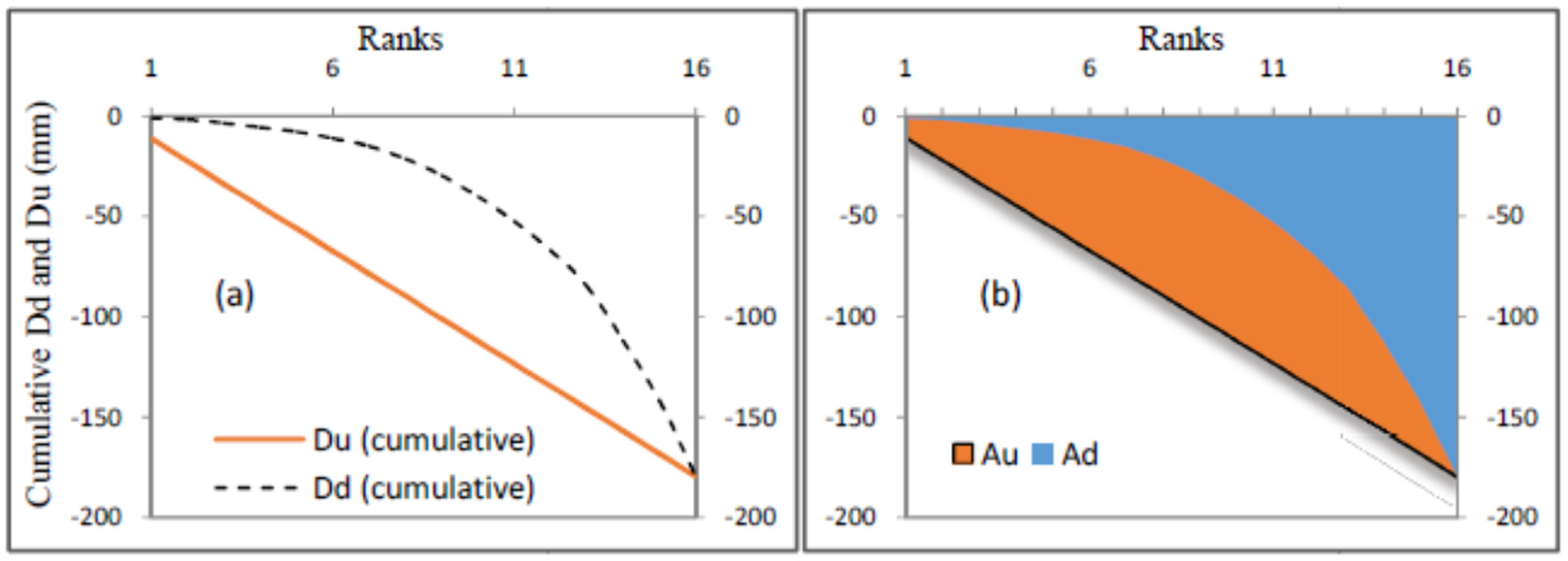
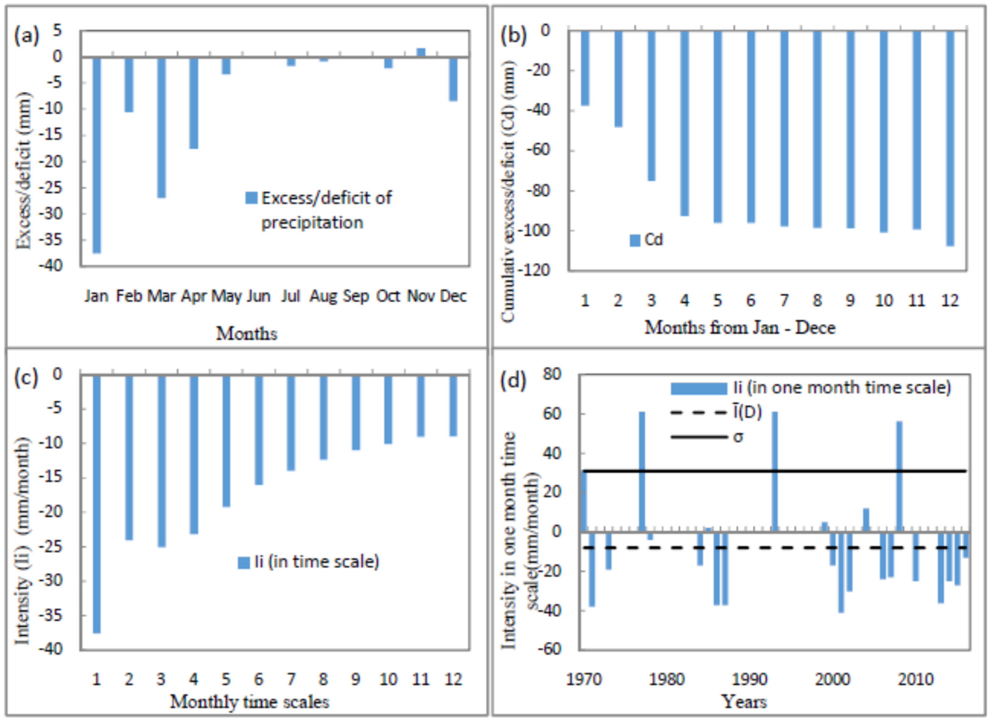
2.2.7. Standardized Precipitation Deficit Distribution (SPDD)

The stepwise procedure to analyze drought intensity, duration and magnitude relationships is described below.

Identification of Excess and Deficit Periods

The wet and dry spells are usually identified from the precipitation series by segregating them into SPI values. Further, the dry spells are analyzed based on monthly precipitation data. The excess and deficit (D_d) of precipitation per month is calculated by deducting the mean monthly precipitation (X_mean) from the monthly precipitation (X_i). Furthermore, excess and deficit are separated. The deficit (D_d) values are arranged in descending order. The present study aims to extract the excess and deficit precipitation periods from the X_i series. The analysis is desired to be quantitative and physically justifiable and transferable through space and time. The threshold of X_i = 0 is selected, as it implies a perfect balance. The excess period is defined as the period of positive X_i values, accounting for the water excess, whereas the deficit period is defined as the negative values, representing the dry period [48].

Derivation of Uniformity Coefficient

The magnitude of the precipitation deficit should be uniformly distributed to utilize the available water effectively [48]. The uniformity coefficient (U_c) is needed to quantify the uniformity of a distribution. Figure 3 is depicted to explain the derivation of U_c for a hypothetical deficit period of a dry spell in R-1. The dashed line in Figure 3a represents the average magnitudes of the uniformity distribution (D_u) corresponding to the respective values of D_d. D_u, for a given deficit period with duration, L, is calculated as:

$$D_u=\frac{\sum _{i=1}^L{D}_{di}}{L}$$

(9)

for the ideal scenario of uniformity, the cumulative sums of D_d and D_u are plotted in Figure 3a, to estimate the areas A_d and A_u under the lines, respectively. The variation between the areas A_u and A_d as shown in Figure 3b is a measure which is not uniform in the system. The area variation per unit is subtracted from 1, which defines the uniformity coefficient (U_c) as derived:

$$U_C=1-\frac{A_u-A_d}{L}$$

(10)

The U_c always ranges between 0 and 1, and it is reduced towards zero, when the nonuniformity increases in a system.

Computation of Refined Deficit Aggregate

In a dry spell, the magnitude of precipitation deficits (M) is obtained from the D_d series. The dry spell includes n dry months or deficit periods. The dry spells’ magnitudes M₁, M₂, …, M_n with durations L₁, L₂, …, L_n, respectively, are derived as:

$$M_i=\sum _{i=1}^{Li}\left(D_{di}\right)$$

(11)

The months with D_d = 0 are included in the wet period since it indicates the balance of mean precipitation with the respective value. The dry spell aggregate D_d is refined by the distribution of magnitudes within the dry spells. The refined aggregate (D_m) is calculated as:

$$D_m=\frac{\sum _{i=1}^n{M}_i{L}_i{U}_{ci}}{\sum _{i=1}^n{L}_i}$$

(12)

where n is the number of dry spells, U_ci is the set of uniformity coefficients of the dry spells.

2.2.8. Drought IDF Analysis

This analysis describes the IDF curves to be the information tools for surface and groundwater resources in Afghanistan. The resources are periodically recharged in each of the years after the severe dry year. Thus, we use the IDF curves for a one-year time scale. The monthly precipitation excess/deficit values of 1, 2, 3, …, 12 month time scales are used to analyze the precipitation deficit intensity [31].The monthly precipitation excess/deficit values are arranged for a one-year time lag of all dry years during (1971–2016), as presented in Figure 4a, which includes the monthly excess/deficit values of the 1971 dry year of R-1.Themonthly cumulative values of excess/deficit were prepared and are represented in Figure 4b. The cumulative deficit (C_d) values from the month of January to December are the sum deficit in each time scale. The C_d values divided by the order of the month result as deficit intensity (I_i) (mm/month) at a time scale (Figure 4c), and derived as:

$$I_i=\frac{C_{di}}{L_i}$$

(13)

where L and i are the length and series of time scales. Furthermore, the one-month time scale intensity from 1970 to 2016 is plotted in Figure 4d. The mean values of drought intensity (${\overline{I}}_D$) and standard deviation (σ) of each time scale are calculated from the drought intensity of the time scales in all the dry years. The black dashed line in Figure 4d shows ${\overline{I}}_D$, and is calculated as:

$${\overline{I}}_D=\frac{\sum _{j=1}^N{I}_{\left(i\right)j}}{N}$$

(14)

where N is total number of years and j is the series of years. In Figure 4c, the black line illustrates σ of the one-month time scale during all the dry years. The σ is estimated for all time scales. Finally, the drought intensity (I_D) for each time scale and return period was estimated according to Chaw et al. [49] which is a known general model for hydrologic frequency analysis.

$$I_D={\overline{I}}_D+K\sigma$$

(15)

The K factor would be calculated for each of the frequencies of 10, 25, 50, and 100 years of return periods (T). In addition, the relationships of I_D and T can be analyzed using linear regression in the logarithmic graphs, the factors (a) and (b) for the logarithmic Equation (16) will be estimated at different time scales and return periods for the classified homogeneous regions.

$$I_D=a\ln \left(T\right)+b$$

(16)

3. Results

3.1. Identification of Homogeneous Regions

The data quality control analysis employs the discordancy measure (D_i) which highlights the discordant sites in the group. The D_i values were estimated using the L-moments statistics and are presented in

Table 3. L-moment parameters and discordancy index for precipitation stations.

Regions	Station No.	Station Name	MAP (mm)	SD	τ2	τ3	τ4	Di
R-1	1	Lashkargah	150	59	−0.06	0.95	−0.61	0.101
	2	Kandahar	198	81	−0.04	1.39	−1.42	0.153
R-2	3	Farah	152	60	−0.07	0.54	−0.27	0.038
	4	Adraskan	228	70	−0.05	0.24	−0.53	0.001
	5	Herat	236	73	−0.05	0.20	−0.48	0.001
	6	Qadis	272	76	−0.04	0.00	−0.64	0.008
R-3	7	Ghazni	451	110	0.98	−0.87	0.96	0.243
	8	Karizimir	484	111	0.99	−0.86	0.94	0.247
	9	Pul-i-Surkh	491	115	1.00	−0.85	0.93	0.248
	10	Gardandiwal	493	108	0.98	−0.88	0.95	0.247
	11	KhwajaRawash	505	116	0.99	−0.86	0.94	0.247
R-4	12	Shiberghan	208	39	0.03	−0.12	0.33	0.000
	13	Mazar-i-Sharif	242	45	0.04	−0.12	0.38	0.000
	14	Maimana	281	58	0.01	−0.01	1.18	0.024
	15	Kunduz	335	63	0.04	−0.18	0.54	0.000
	16	Baghlan	349	67	0.04	−0.13	0.50	0.001
	17	Faizabad	522	91	0.02	−0.24	0.89	0.000
R-5	18	Lal-Sarjangal	349	81	0.03	0.30	1.16	0.081
	19	North Salang	547	111	0.05	0.18	0.55	0.023
	20	Tang-i-Sayedan	563	136	0.07	0.28	0.38	0.030
	21	Khost	595	130	0.06	0.36	0.46	0.047
	22	Jalalabad	689	148	0.06	0.37	0.40	0.045
R-6	23	Ghalmin	337	75	0.00	478.34	−1493.48	5.882

. Notably, the high D_i value (5.882) for the Ghalmin station indicates the station’s substantial deviation from other stations related to their frequency distribution. As mentioned in Section 2.2.1, D_i > 1.64 is considered as discordant. Conversely, the D_i values for all other regions identified as homogeneous (R-1, R-2, R-4, and R-5) are within the critical threshold of 1.64. The stations in the R-3 region (central part of the country) exhibit higher D_i values relative to the other regions, which underscores the distinctive characteristics and potential anomalies of the region.

3.1.1. Homogeneous Regions

The homogeneous regions are formed by grouping the sites that satisfy the homogeneity of similar frequency distributions using the variations of the coefficients L-CV, L-skewness, and L-Kurtosis. The L-moment parameters, with the MAP and standard deviation for all the stations are presented in Table 3. The L-moment parameters were plotted (see Figure 5a,b) for heuristic analysis, and it is pertinent to observe that the data points corresponding to the Ghalmin station fall beyond the range delimited by the plots. Additionally, the scattered distribution of data points from other stations reveals that the stations are not homogeneous. Thus, the stations were grouped into six sub-regions (R-1, R-2, R-3, R-4, R-5, and R-6) according to their frequency distribution characteristics; however, R-6 which contains the Ghalmin station, was discordant and is not shown in Figure 5. Spatial distribution of the homogeneous regions is shown in Figure 6.

3.1.2. Homogeneity Test

The homogeneity criteria are used to assess whether the regions are homogeneous based on the similarity of frequency distributions from the area of the exact scale factor. The heterogeneity measure (H) is calculated for each homogenous region derived above based on Hosking et al. [9] and presented in

Table 4. Regions and their homogeneity.

Regions	No of Stations	Abs (H)	Homogeneity Type
R-1	2	0.49	Homogeneous
R-2	4	0.55	Homogeneous
R-3	5	0.41	Homogeneous
R-4	6	0.79	Homogeneous
R-5	5	0.44	Homogeneous
R-6	1	1.86	Possibly heterogeneous

. From the table it is evident that all the regions (except R-6) are acceptably homogenous (Abs (H) < 1). Since the H value for R-6 is between 1 and 2, the region can be considered as possibly heterogeneous.

3.2. Selection of a Suitable PDF

The performance evaluation was conducted on the candidate distribution functions fitted to each homogeneous region through the goodness of fit measure, based on L-moment ratios. The candidate distributions considered are: (i) Generalized Pareto distribution (GEP), (ii) Gumbel distribution (GUM), (iii) Exponential distribution (EXP), (iv) Lognormal distribution (LN), and (v) Normal distribution. The goodness of fit measure method [7,8] was used to estimate the parameters. Figure 7 shows the Z^DIST values for each region for all the candidate distributions. The horizontal dashed line (Z^DIST = 1.64) defines good fit distributions. Clearly, the GEP distribution function presents a good fit in all the regions except R-3, while the GUM function emerges as a good fit for R-3. For all the regions, the results of this study proposed GEP and GUM distribution functions and the detailed description of the functions are presented by [39].

3.3. Standardized Precipitation Index

The average annual precipitation from 1970 to 2016 for each homogeneous region (R-1, R-2, R-3, R-4, R-5, and R-6) was used to estimate the SPI [21] and is shown in Figure 8. This shows the temporal sequence of wet and dry periods in the homogenous regions for the years considered. Among the regions, R-1 and R-2 fall under the arid climate and the remaining regions experience mostly a semi-arid climate. Notably, from Figure 8 it is evident that the variations of SPI in the R-1, R-2, and R-6 regions are high, ranging from drought to wet conditions. The average duration of the variation shows low resiliency from the dry to the wet condition. In contrast, remaining regions (R-3, R-4, and R-5) exhibit high variation and higher resiliency. It means that the semi-arid climate regions have more resilience relative to the arid climatic regions. This may be due to a lesser amount of annual precipitation in the arid and a higher precipitation in the semi-arid climatic regions.

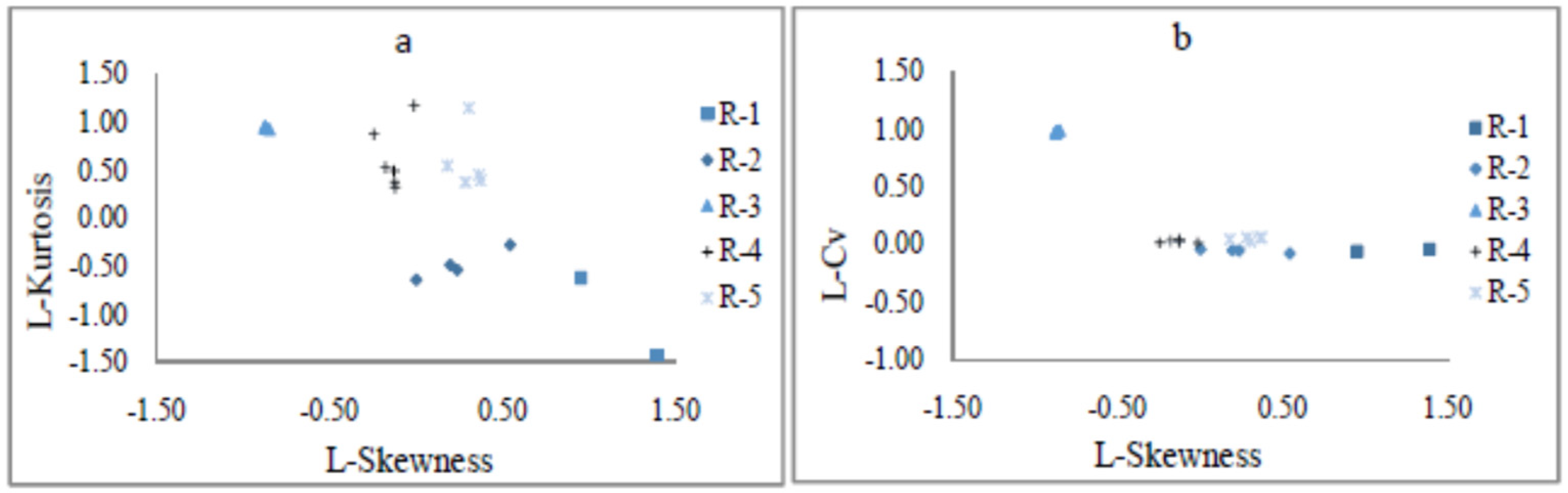
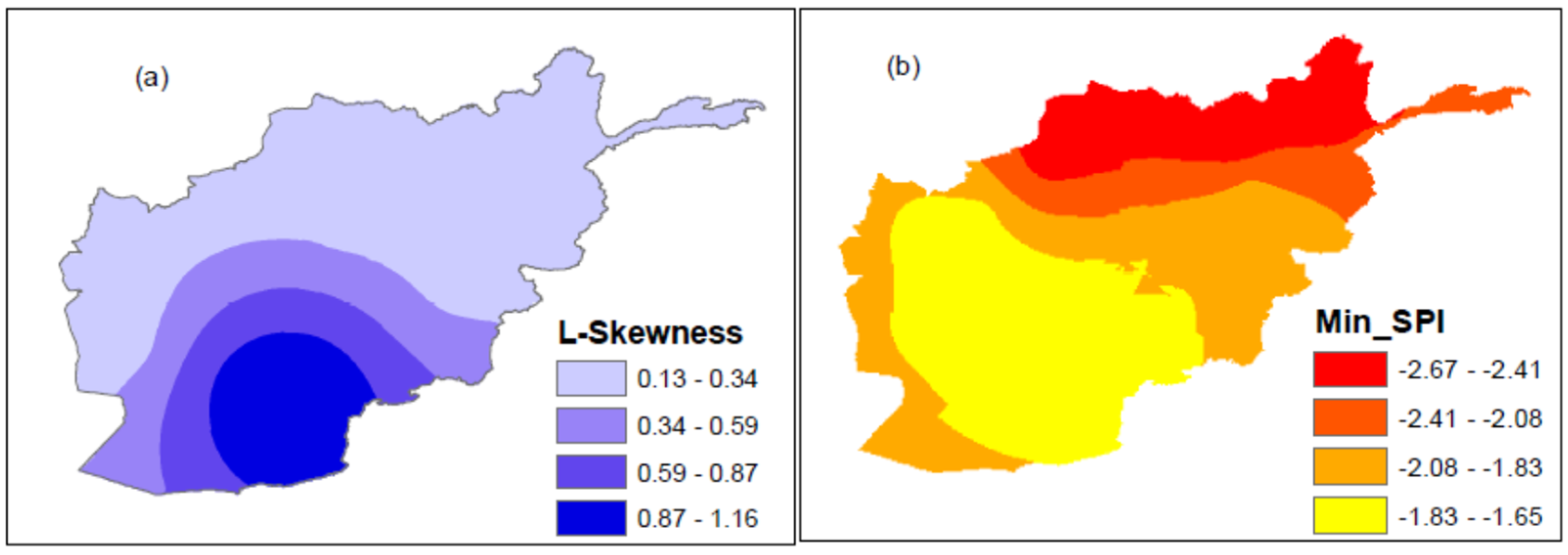
3.4. Regional Drought Severity Relation to L-Moment Parameters

In this section the regional drought severity was quantified while highlighting the significance of L-moment parameters. As few homogeneous regions exhibit similar behavior, they are combined into a single region. The exponential decay relationship between MAP and L-moment parameters has been observed worldwide by several authors [7,8,9]. In this study, the L-skewness factors of homogeneous regions R-1 to R-5 were obtained from the L-moment statistics of SPI values and the spatial maps of absolute values of the L-skewness and min SPI are shown in Figure 9. However, region 6 (R-6) is considered as possibly heterogeneous, and thus, excluded from this analysis. It is noteworthy that the average SPI values for all the regions were zero. Thus, we have used the minimum values of SPI such as −1.67, −1.78, −1.86, −2.64, and −1.98 of regions 1, 2, 3, 4, and 5, respectively. Exponential equations were used to capture the relationship between the L-skewness factors and minimum SPI values of the regions. The derived values for the parameters in Equation (4) are α = 5.12, β = 1.39, and δ = 0. The min SPI values of the regions pointed out extreme drought conditions in the R-4 region, which spanned the northeastern and eastern parts of the country. Additionally, a compelling observation indicating a direct correlation between decreasing L-skewness and increasing drought severity is visible from the analysis. Generally, the drought severity decreases from the east to west of the country. In contrast, L-skewness increases to the west of Afghanistan. It means that the value of the L-moment parameter is high in the arid-climate desert areas.

3.5. Drought Frequency Analysis

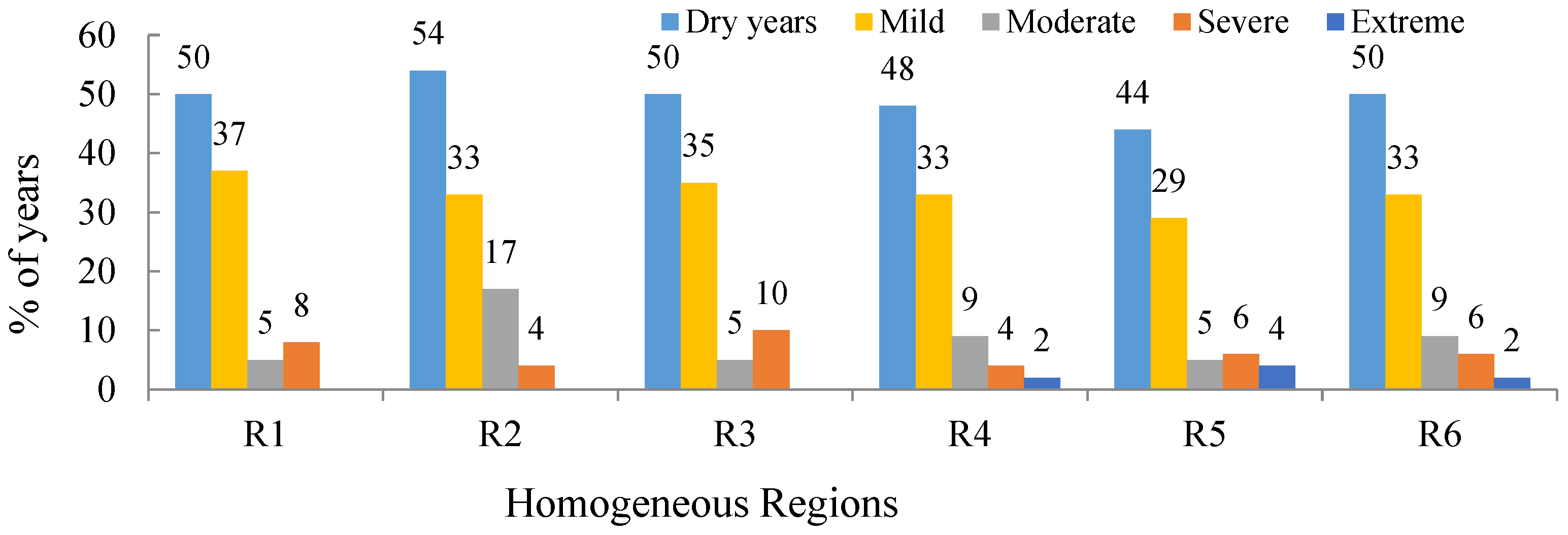
3.5.1. Percentage of Dry Years

The annual SPI values were plotted against the probability of occurrence as a percentage of years and are shown in Figure 10. Additionally, occurrence of different severity droughts in each homogenous region is shown in Figure 11. While analyzing the 47 years of annual precipitation, drought years ranged from 44 to 54% for various regions. Among these, the high percentage of dry years was witnessed in the arid climate region (R-2) with 54% of the years under drought (mild: 33%; moderate: 17%; severe: 4%) compared to the semi-arid region (R-5) which experienced drought during 44% of the years (mild: 29%; moderate: 5%; severe: 6%; extreme: 4%). R-3 faces frequent severe drought (10% of the years), and R-2 faces frequent moderate drought (17% of the years). Similarly, mild drought is more frequent in R-1 (37% of the time) compared to the least frequent region of R-5 (29% of the years). R-3 and R-5 regions are densely populated areas in which the severe droughts affect the socioeconomics of the residences. In addition, these regions are upstream of the Hilmand and Kabul River basins which cover all southern areas of the country. Approximately half of Afghanistan is getting affected by severe droughts, mainly the water supply system and groundwater storage.

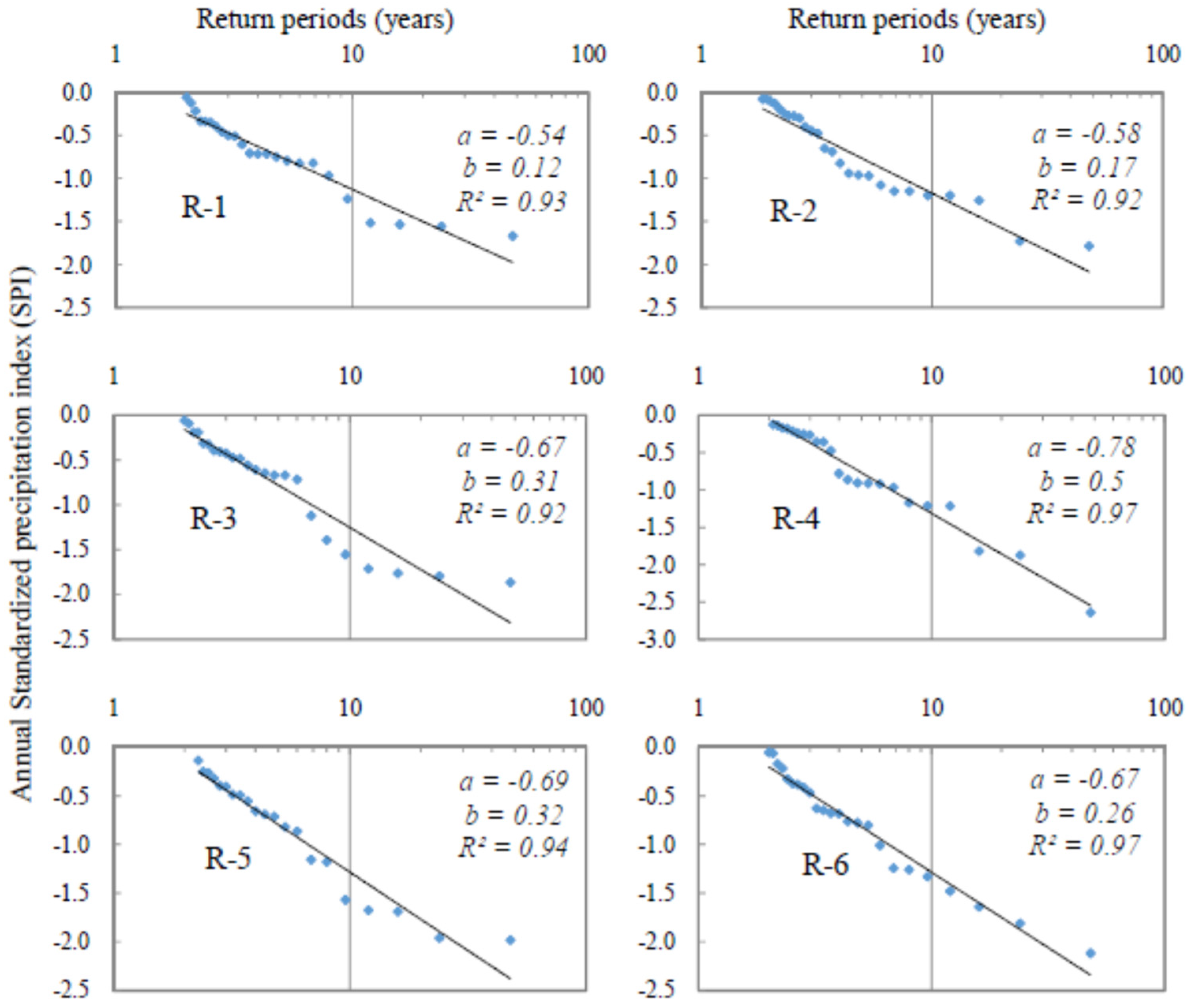
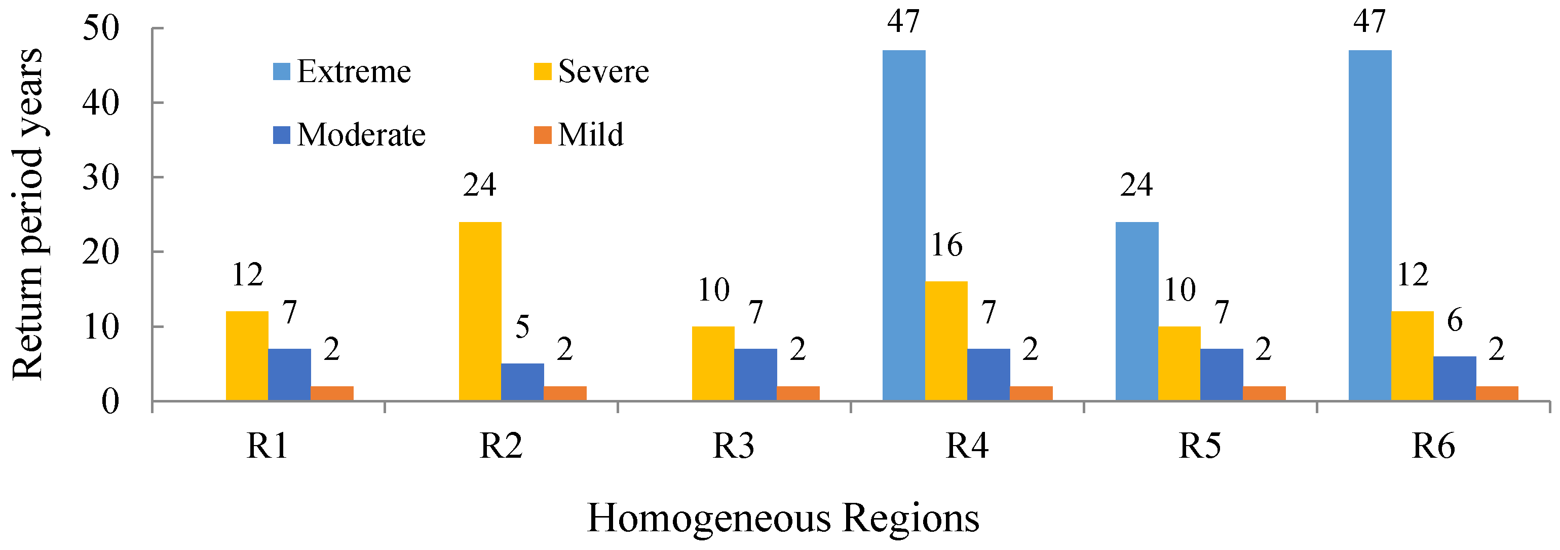
3.5.2. Drought Severity and Return Period

The frequency analysis of SPI values during dry years can be used to assess the recurrence intervals (or) return periods of various drought categories, namely mild, moderate, severe, and extreme as categorized by [18] and the same is shown in Figure 12. The results showed that once in two years, mild drought was experienced in all the regions. The return periods of moderate, severe and extreme drought events are shown in Figure 13. However, the drought frequency and severity levels (e.g., extreme events) could potentially become more potent in future due to climate change [50]. Consequently, comprehending the implications and management responses becomes even more imperative. The drought frequency serves as the key factor in the decision-making process for policymakers. The imminent challenge to the future drought policy is formulating adaptation plans for the anticipated more frequent, severe and prolonged drought events and managing the water scarcity [51]. One possible avenue lies in increased irrigation efficiency and water-saving farm practices, which will balance both water supply and demand. Increasing irrigation efficiency not only diminishes the risk but also facilitates the restoration of water resources for the environment [50].

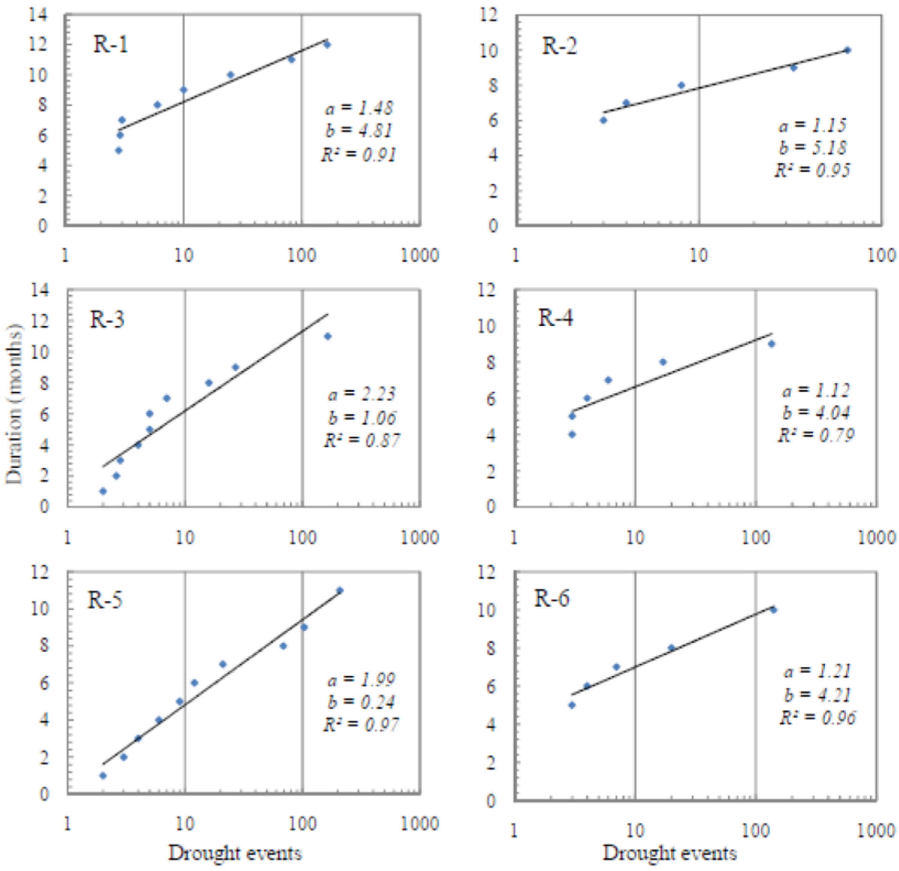
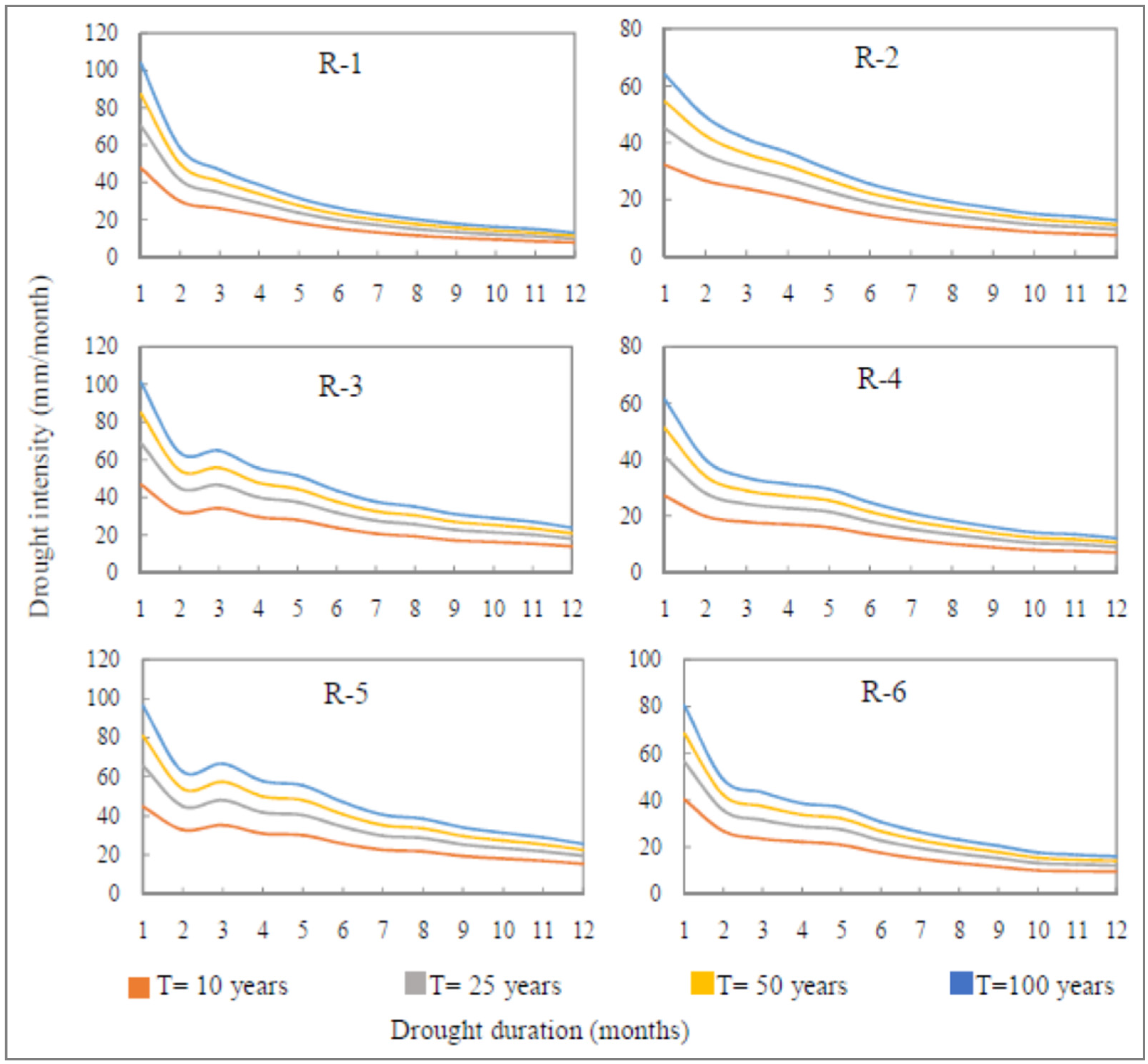
3.5.3. Drought Duration and Frequency

The prolonged droughts affect the socioeconomics of the population and environment in the country. Duration of drought is the continuous period during which the SPI remains persistently below the fixed threshold level of zero. The SPI was designed according to [18] to separately analyze the frequency of drought episodes. Results are presented in Figure 14. The frequency of the longest drought durations were 164, 65, 164, 135, 208, and 141 events in regions R-1, R-2, R-3, R-4, R-5, and R-6, respectively. Moreover, the long-term durations of drought were12, 10, 11, 9, 11 and 10 months in regions 1, 2, 3, 4, 5 and 6, respectively. This long-term drought occurred from 1998 to 2005. Furthermore, the linear regression of drought duration and frequency, estimated a lower slope factor of 1.12 in R-4, which has high resiliency when related to the other regions, as shown in Figure 8. The slope factor increased to 2.23 and 1.99 in regions 3 and 5, respectively, while the regions had a higher amount of annual rainfall. The regions 1, 2 and 6 are included in the arid climate area and had a lower resiliency of dry and wet episodes due to the long duration of the drought, the regions resulted in lower factors of around 1.48, 1.15 and 1.21, respectively.

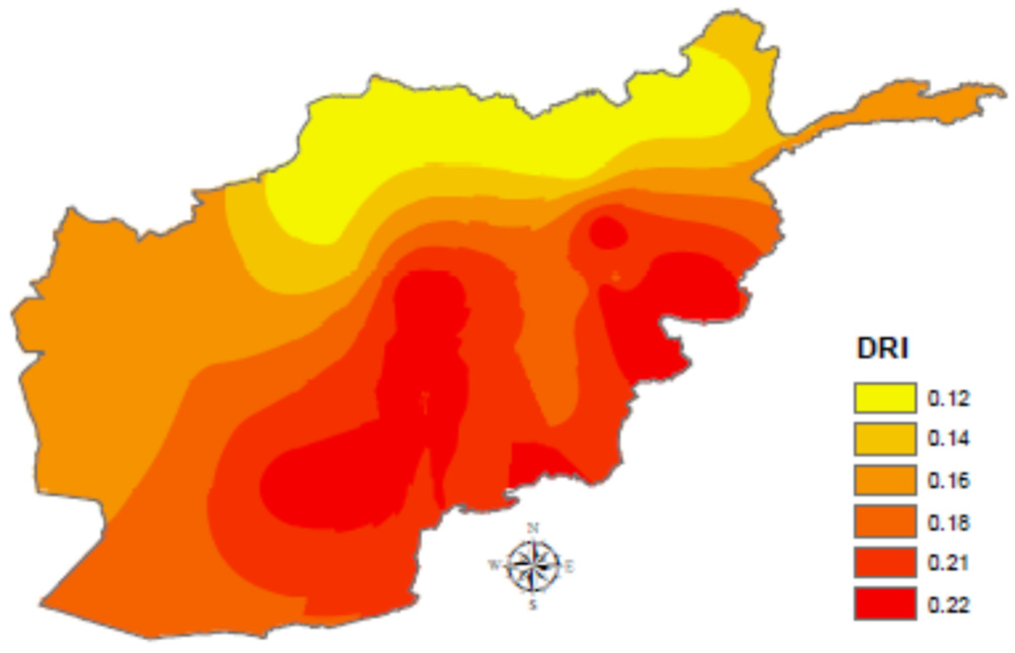
3.6. Drought Risk Analysis

The drought hazard indicator (DHI) was analyzed using the designated droughts for each of the homogeneous regions. Using Equation (6), the DHI values were estimated for the homogenous regions. The DHI values for R-1, R-2, and R-3 were 0.27, 0.28, and 0.37, while, slightly increased values of 0.4, 0.4, and 0.46 were estimated for R-3, R-4, and R-5, respectively. This disparity stems from the higher probability for the occurrence of drought events in semi-arid climates, compared to arid climate regions. Additionally, the drought variability indicator (DVI) was calculated based on the water demand from the available water resources. The DVI values were 0.79, 0.56 for R-1, and R-2, while the values declined to 0.46, 0.29, 0.47, and 0.39 for R-3, R-4, R-5, and R-6, respectively. Higher DVI values in arid climates are a consequence of prolonged drought events coupled with substantial water demand. In summary, DVI provides insights about how water demand copes with drought, while DHI provides potential drought risk.

Furthermore, the regional drought risk indicators (DRI) were spatially mapped in the study area as shown in Figure 15. The minimum value of DRI was 0.12 in R-4 which is in the northeast semi-arid climate area. Whereas R-1 and R-5 in the southwest and southeast of the country, resulted in an increase in DRI, having values of 0.21 and 0.22, respectively. The spatial variation of DRI (Figure 15) depicts a high drought risk in southern areas of Afghanistan indicating high water demand and a higher probability for drought occurrence. While the southeast area receives moderate precipitation during the summer due to the effects of the Indian monsoon, the southern area of the country is cold and desert [38].

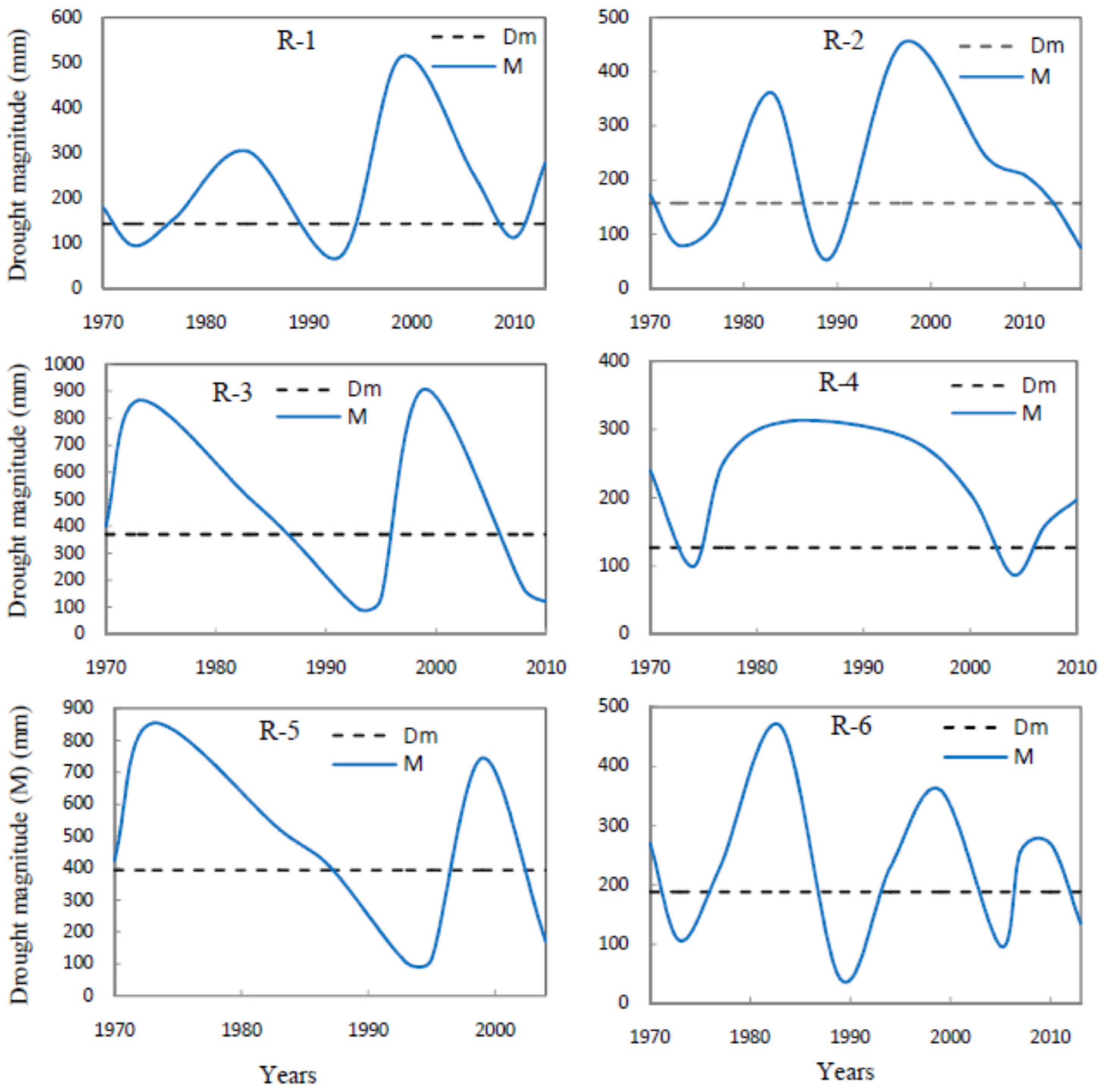
3.7. Drought Magnitude Distribution

As mentioned above, drought events have occurred at different intensities, durations and frequencies in the study area during the analysis period from 1970 to 2016. To comprehensively characterize these fluctuations relative to their mean values, this study uniformly distributed the deficit precipitation (D_m) using the uniformity coefficient (U_c) [48]. Further, the deficit precipitation (D_u) corresponding to the uniform distribution, was indicated for each drought episode. Temporal variations in drought intensity of different drought incidents were analyzed. The U_c and D_u showed minor variations in R-1 due to the arid climate in the region. In contrast, the semi-arid climate regions displayed higher variations in U_c and D_u. An intense drought spell occurred in R-4 and R-6 during 1980–1990 (see Figure 8). However, in the results of this study, a long-term drought happened during 1998–2005 in most of the regions, while the years 2000 and 2001 had a severe drought. The higher deficit intensity and lower uniformity determined a more resilient deficit in R-3 and R-5. And, higher uniformity and intensity in R-4 and R-6 showed a lower resiliency of the deficit distribution.

Furthermore, D_u approaches D_m, when U_c increased toward one. In addition, the values of M reached D_m when U_c became equal to one [48]. The (blue line) M above (black dashed line) D_m showed critical drought episodes, and below are less severe or short-term droughts (Figure 16). The regions resulted in different distributions in drought magnitudes considering their climate variations [38]. The consequences of this analysis depicted long-term and severe drought episodes in R-1 and R-2 around the year 2000, in contrast to the severe drought that happened around 1970 and 1980 in R-3, R-5 and R-6. A severe and long-term drought episode during the years 2000–2021 occurred in R-3. The lesser values of D_m in R-1 and R-2 are due to the arid climate in these regions [52]. And R-4 had a low D_m, because of the nonuniformity and lesser degree of drought magnitude.

3.8. Drought IDF Analysis

The short-term droughts were analyzed for agro-climatic design [35]. The short duration of the drought in the long term could affect the rainfed agriculture in Afghanistan extremely. Moreover, irrigated agriculture is related to the reservoirs which store water in the winter months. This needs planning according to a 12 monthly time-scale drought analysis. The mean values of drought intensity (${\overline{I}}_D$) and standard deviation (σ) for 1, 2, 3,…12 month time scales and in the identified regions, were estimated from the precipitation deficit values. In the study area, high precipitation generally occurs in Jan, Feb, Mar, and Apr. The high values of the precipitation deficit take place in these months of the drought years which are a result of high values of drought intensity. R-4 exists in the northeast of the country which has a semi-arid climate, the region had a quite uniform distribution of precipitation in all months during the year, and drought effects were nearly uniform in all months. Thus, the drought intensities had fewer variations in all the time scales. Furthermore, the standard deviation of the precipitation deficit was decreased when the drought time scale increased. However, the K factor is a function of the return period. In this study, the estimated values of K were 1.304, 2.043, 2.592, and 3.136 for frequencies of 10, 25, 50, and 100 years, respectively. The factors are increased with an increasing return period. Therefore, the drought intensity can be increased by enhancing the K factor.

Drought intensity for various time scales in homogeneous regions of different climate areas was calculated according to [49]. The drought IDF relationships were developed for different climatic regions in Afghanistan which could be used for hydro-climatic and agro-climatic design and planning. The drought IDF curves are presented in Figure 17. The overall results of the curves showed high drought intensity when the return period increases. The variations in drought intensity increased when the frequency and drought duration decreased. The drought intensity at the one-month time scale ranged between 3–104, 7–64, 3–101, 0–62, 4–96, and 8–81 mm/month in R-1, R-2, R-3, R-4, R-5, and R-6, respectively. Furthermore, an increase in time scale decreases the standard deviation. This resulted in a decrease in the variations of intensity with increasing frequency. The graphs showed fewer variations of intensity in investigations of 12 month time scales. The frequencies of 10, 25, 50, and 100 years showed that intensity significantly decreased when the time scale increased. In the 12 month time scale, when frequency increased from 10 years to 100 years, the variations in intensity were calculated at a range of 4–13, 4–13, 6–24, 3–12, 7–26, and 4–16 mm/month in regions 1, 2, 3, 4, 5, and 6, respectively. The high degree of variation in intensity in the 12 month time scale were estimated in R-3 and R-5, which are located in the east of Hilmand and Kabul river basins. It means that severe drought can occur in the regions for a long time.

The logarithmic Equation (16) is used to calculate drought intensity using the return period. The factors of (a) and (b) for different regions and time scales were estimated by linear regression analysis with R² = 0.998.

Table 5. The factors for the logarithmic equation in different regions and various time scales.

Month Scale	R-1		R-2		R-3		R-4		R-5		R-6
	a	b	a	b	a	b	a	b	a	b	a	b
1	25.86	−13.78	14.6	−2.42	24.98	−12.53	15.77	−10.27	23.73	−11.6	18.43	−3.43
2	13.14	−1.34	10.37	1.97	14.53	−2.41	9.26	−2.1	13.66	0.51	10.1	2.84
3	9.516	3.41	8.04	4.79	14	0.97	7.26	0.63	14.43	1.1	9.05	2.17
4	7.57	4.32	7.2	3.88	11.93	1.13	6.6	1.38	12.39	1.52	7.49	4.55
5	6.14	3.71	6.03	3.34	10.78	2.41	6.22	1.32	11.72	2.3	7.32	3.72
6	5.11	3.09	5.03	2.78	9.06	2.38	5.22	1.14	9.81	2.48	6.1	3.1
7	4.43	2.69	4.31	2.39	7.78	2.27	4.38	1.22	8.26	3.1	5.23	2.66
8	3.89	2.35	3.77	2.08	7.25	2.11	3.81	1.13	7.7	3.59	4.57	2.33
9	3.46	2.09	3.35	1.85	6.41	1.99	3.32	1.1	6.71	3.54	4.06	2.07
10	3.12	2.04	2.94	1.73	5.87	2.38	2.89	1.16	6.1	3.81	3.52	1.78
11	2.91	1.67	2.79	1.44	5.34	2.73	2.67	1.36	5.48	4.05	3.21	2.14
12	2.32	2.34	2.39	2	4.55	3.2	2.4	1.39	4.71	4.32	2.97	2.51

presents the factors prepared to determine drought intensity through the equation in various regions and time scales. Generally, the factors are high at the one-month time scale and decrease when the time scale increases. The highest value of the slope factor (a) was 25.86 in R-1 for a one-month time scale. This shows the high variation of drought intensity between 10 years and 100 years of return periods. In contrast, the lowest value of the slope factor was 2.32 in R-1 for the 12-month time scale, which illustrated that there is less variation of intensity with an increasing return period.

4. Discussion

A lack of data in developed countries is a challenge for researchers to analyze various climatic, environmental, and social aspects. Therefore, this study used a framework to analyze drought characteristics by considering the drought risk assessment with “information tools for water resources management planning” especially in a scarce data region like Afghanistan. The country has a complex climate [38], thus we identified the homogeneous regions related to their similar drought frequency as represented in (Figure 6). Various homogeneous regions were identified such as southwest, southeast, northwest, northeast, and central parts, which have different climates. Moreover, by employing the drought hazard indicator (DHI) and drought vulnerability indicator (DVI), comprehensive drought risk assessment can be achieved. A conceptual framework was used with a combined role of drought hazard and drought vulnerability to assess the spatial drought risk for the homogeneous regions, as presented in (Figure 15). The higher drought risk indicators 0.21 and 0.22 were exposed to very high risk in the southwest and southeast of Afghanistan which is the result of the occurrence of a long and severe drought. The central part of the country which has a semi-arid climate and highland area that feeds all river and water resources in Afghanistan is also in high drought risk regions, that could impact on 80% of the population in the country whose lives are related to agriculture [37]. According to Figure 10, approximately 50% of the years were dry which includes mild, moderate, and severe drought. Mild and moderate drought affects 1.3 million ha of rainfed agriculture, while the severe dry years effect 2.6 million ha of irrigated agriculture and all water resources in Afghanistan.

Furthermore, drought is a long-lasting phenomenon, and needs preparedness in planning to mitigate drought risk and manage the available water resource balance. For this, the drought magnitude using the precipitation deficit should be uniformly distributed to utilize the available water effectively [48]. Thus, the uniformity coefficient (U_c) is required to quantify uniformity of the precipitation deficit distribution (D_m). In this study, various D_m values were estimated in different climatic regions related to the U_c variations in arid and semi-arid climate areas. The values of D_m were lower in arid climate areas due to minimum values of U_c (Figure 16), and the drought magnitude being higher in R-3 and R-5in the southeast and central parts of the country which have a highland and semi-arid climate. From these regions, the snow melted water flows toward the arid climate and the downstream area in the summer season. The high drought magnitude in these regions could affect all surface and groundwater resources in Afghanistan. That would have serious impacts on food demand and over-exploitation of groundwater resources [1].

However, droughts affect both surface and groundwater resources and can lead to impacts on the economy in the country. Thus, understanding droughts has a significant role in water resource planning and management [53]. The drought IDF relationships analysis is one of the statistical investigations to understand future drought risk, potential changes of drought properties and characteristics [33]. The drought IDF curves are important tools not only in studying drought characterization for research but also for easily transferring drought information to end users for practical purposes [31]. Therefore, this study estimated the regional IDF curves which are the important tools for agro-climatic and hydro-climatic planning for drought risk mitigation, as depicted in (Figure 17). The curves can be used for agriculture and water resource planning in the same way that the precipitation IDF curves are used in the hydrological design. The drought intensity in the short-term time scale affects seasonal agriculture, while the long-term drought influences agriculture and water resources in the country. For design purposes, the IDF relationships can be used for a long time to investigate severe and extreme drought. And planning of agriculture development is related to upgrading the agro-climatic and hydro-climatic design which is affected by meteorological extremes, such as droughts [35]. Furthermore, with the use of drought IDF curves, it is projected that the permanent and destructive effects of drought can be understood [32]. The final information in the form of a precipitation deficit was provided to the end-users. This information can be used for advanced planning against drought. Furthermore, understanding drought intensity-duration-frequency (IDF) curves provides critical insights into drought characteristics. Overall, this framework will contribute to enhancing the knowledge that spatially identifies the most affected region related to drought vulnerability and resiliency, and identify the regions of high risk where the drought impacts on the socioeconomics of the population. This aids in developing effective drought mitigation measures and sustainable water resource management in Afghanistan. In order, based on Equation (16), the drought intensity is obtained throughout the return periods using the provided factors in Table 5 in different time scales and various regions of the study area.

Overall, the analysis showed that the south and the central areas of the country arevulnerable to drought risk in the future. The results from this study contribute to the findings of studies conducted, such as those [3,54,55] in the Central Asian region [36,38] in Afghanistan. The outcome of this study would be useful in providing a scientific solution for better management of the scarce water resources of Afghanistan. Furthermore, this would add scientific value to the current understanding and modeling of drought, especially in the arid regions where better management of water resources is of paramount importance.

5. Conclusions

This study introduced a framework to analyze regional drought based on RDRA and RD-IDF curves for a scarce data region in Afghanistan. The homogeneous regions were identified based on L-moment statistics. We used the combined role of DHI and DVI to estimate RDRA in each of the homogeneous regions. The drought magnitude was investigated by SPDD. And, the RD-IDF relationships were quantified based on GM-HFA using the monthly rainfall deficit data (1970–2016) at the regional level. In the results of this study, partitioning of the sites by similar frequency divided the country into six homogeneous regions. Generally, a high occurrence probability of mild and moderate drought showed that 1.3 million ha rainfed agriculture is affected in more than 50% of the years in all of Afghanistan. Consequently, the spatial map of drought risk exposed high drought risk indicators of 0.21 and 0.22 in the southwest and southeast of Afghanistan. Also, the central part of the country which is the upstream and main water resource for the south and west regions was included in the high drought risk area. That can affect the socioeconomics of 80% of the population whose lives are related to agriculture. A higher drought magnitude in R-3 and R-5 in the southeast and central parts of the country could impact on 2.6 million ha of irrigated agriculture, water supply systems and groundwater resources. However, drought needs preparedness and drought risk mitigation planning to reduce the risk. For this, management is required for available water resources and agriculture. Therefore, this study identified information tools in the form of IDF curves for the classified regions. The curves can be used for hydro-climatic and agro-climatic design and planning concerning drought in Afghanistan. In the south and central areas of the country, for a one-month time scale, the analysis showed high variations in drought intensity when increasing the return period that would enhance the effects of drought on rainfed agriculture in the future. However, the results showed fewer variations in drought intensity when the return period increased from 10 years to 100 years and the time scale increased to 12 months. This can affect the water resources of the country in the future. In addition, the factors in the equations of intensity and return period were prepared for the calculation of drought intensity through return periods over various time scales and different regions of the country. The results of this study can be essential information for end users to create advanced planning for drought effects mitigation based on different regional levels in Afghanistan.

References

1. Hosseini, A.; Ghavidel, Y.; Farajzadeh, M. Characterization of drought dynamics in Iran by using S-TRACK method. Theor. Appl. Climatol. 2021, 10, 1007. [Google Scholar] [CrossRef]
2. Sa’adi, Z.; Shahid, S.; Ismail, T.; Chung, E.S.; Wang, X.J. Distributional changes in rainfall and river flow in Sarawak, Malaysia. Asia Pac. J. Atmos. Sci 2017, 53, 489–500. [Google Scholar] [CrossRef]
3. Ahmed, K.; Shahid, S.; Chung, E.S.; Ismail, T.; Wang, X.J. Spatial distribution of secular trends in annual and seasonal precipitation over Pakistan. Clim. Res. 2017, 74, 95–107. [Google Scholar] [CrossRef]
4. Hadi Pour, S.; AbdWahab, A.K.; Shahid, S.; Wang, X. Spatial Pattern of the Unidirectional Trends in Thermal Bioclimatic Indicators in Iran. Sustainability 2019, 11, 2287. [Google Scholar] [CrossRef]
5. ND-GAIN—Notre Dame Global Adaptation Initiative. “Afghanistan”. 2021. Available online: https://gain-new.crc.nd.edu/country/afghanistan (accessed on 6 November 2021).
6. Sarhadi, A.; Heydarizadeh, M. Regional frequency analysis and spatial pattern characterization of dry spells in Iran. Int. J. Clim. 2014, 34, 835–848. [Google Scholar] [CrossRef]
7. Kaluba, P.; Verbist, K.M.J.; Cornelis, W.M.; Van Ranst, E. Spatial mapping of drought in Zambia using regional frequency analysis. Hydrol. Sci. J. 2017, 13, 43475. [Google Scholar] [CrossRef]
8. Núñez, J.H.; Verbist, K.; Wallis, J.R.; Schaefer, M.G.; Morales, L.; Cornelis, W.M. Regional frequency analysis for mapping drought events in north-central Chile. J. Hydrol. 2011, 405, 352–366. [Google Scholar] [CrossRef]
9. Hosking, J.; Wallis, J. Contents in Regional Frequency Analysis: An Approach Based on L-Moments; Cambridge University Press: Cambridge, UK, 1997. [Google Scholar]
10. Santos, J.F.; Portela, M.M.; Pulido-Calvo, I. Regional frequency analysis of droughts in Portugal. Water Resour. Manag. 2011, 25, 3537–3558. [Google Scholar] [CrossRef]
11. Modarres, R. Regional dry spells frequency analysis by L-Moment and multivariate analysis. Water Resour. Manag. 2010, 24, 2365–2380. [Google Scholar] [CrossRef]
12. Yoo, J.; Kwon, H.-H.; Kim, T.-W.; Ahn, J.-H. Drought frequency analysis using cluster analysis and bivariate probability distribution. J. Hydrol. 2012, 1, 102–111. [Google Scholar] [CrossRef]
13. Zhang, Q.; Qi, T.; Singh, V.P.; Chen, Y.D.; Xiao, M. Regional frequency analysis of droughts in China: A multivariate perspective. Water Resour. Manag. 2015, 29, 1767–1787. [Google Scholar] [CrossRef]
14. Núñez, J.; Hallack-Alegría, M.; Cadena, M. Resolving regional frequency analysis of precipitation at large and complex scales using a bottom-up approach: The Latin America and the Caribbean Drought Atlas. J. Hydrol. 2016, 538, 515–538. [Google Scholar] [CrossRef]
15. Palmer, W.C. Meteorological Drought; U.S. Dept. of Commerce: Washington, DC, USA, 1965; Rep. 45; p. 58. [Google Scholar]
16. Palmer, W.C. Keeping Track of Crop Moisture Conditions, Nationwide: The New Crop Moisture Index. Weatherwise 1968, 21, 156–161. [Google Scholar] [CrossRef]
17. McKee, T.B.; Doesken, N.J.; Kleist, J. The relationship of drought frequency and duration to time scales. In Proceedings of the 8th Conference on Applied Climatology; Anaheim, CA, USA, 17–22 January 1993, Volume 17, No. 22.
18. Mckee, T.B. Drought monitoring with multiple timescales. In Proceedings of the Ninth Conference on Applied Climatology, Dallas, TX, USA, 15–20 January 1995; Boston American Meteorological Society: Boston, MA, USA; pp. 233–236. [Google Scholar]
19. Sohrabi, M.M.; Ryu, J.H.; Abatzoglou, J.; Tracy, J. Development of Soil Moisture Drought Indexto Characterize Droughts. J. Hydrol. Eng. 2015, 20, 04015025-1. [Google Scholar] [CrossRef]
20. Quiring, S.M.; Ganesh, S. Evaluating the utility of the Vegetation Condition Index (VCI) for monitoring meteorological drought in Texas. J. Agric. For. Meteorol. 2010, 150, 330–333. [Google Scholar] [CrossRef]
21. Beguería, S.; Vicente-Serrano, S.M.; Reig, F.; Latorre, B. Standardized precipitation evapotranspiration index (SPEI) revisited: Parameter fitting, evapotranspiration models, tools, datasets and drought monitoring. Int. J. Climatol. 2014, 34, 3001–3023. [Google Scholar] [CrossRef]
22. Hoekema, D.J.; Sridhar, V. Relating climatic attributes and water resources allocation: A study using surface water supply and soil moisture indices in the Snake River basin, Idaho. Water Resour. Res. 2011, 47, 536. [Google Scholar] [CrossRef]
23. Wu, H.; Hayes, M.J.; Wilhite, D.A.; Svoboda, M.D. The Effect of the Length of Record on the Standardized Precipitation Index Calculation. Int. J. Clim. 2005, 25, 505–520. [Google Scholar] [CrossRef]
24. Aksoy, H.; Cavus, Y. Discussion of “Drought assessment in a south Mediterranean transboundary catchment”. Hydrol. Sci. J. 2022, 67, 150–156. [Google Scholar] [CrossRef]
25. Yu, J.; Kim, J.E.; Lee, J.-H.; Kim, T.-W. Development of a PCA-Based Vulnerability and Copula-Based Hazard Analysis for Assessing Regional Drought Risk. J. Civ. Eng. 2021, 25, 1901–1908. [Google Scholar] [CrossRef]
26. Intergovernmental Panel on Climate Change. Managing the Risks of Extreme Events and Disasters to Advance Climate Change Adaptation: Summary for Policymakers; Cambridge University Press: Cambridge, UK, 2012; pp. 1–19. [Google Scholar]
27. Kim, H.; Park, J.; Yoo, J.; Kim, T.-W. Assessment of drought hazard, vulnerability, and risk: A case study for administrative districts in South Korea. J. Hydro-Environ. Res. 2015, 9, 28–35. [Google Scholar] [CrossRef]
28. Carrão, H.; Naumann, G.; Barbosa, P. Mapping global patterns of drought risk: An empirical framework based on sub-national estimates of hazard, exposure and vulnerability. Glob. Environ. Chang. 2016, 39, 108–124. [Google Scholar] [CrossRef]
29. Hinkel, J. “Indicators of vulnerability and adaptive capacity”: Towards a clarification of the science-policy interface. Glob. Environ. Chang. 2011, 21, 198–208. [Google Scholar] [CrossRef]
30. Shahid, S.; Behrawan, H. Drought risk assessment in the western part of Bangladesh. Nat. Hazards 2008, 46, 391–413. [Google Scholar] [CrossRef]
31. Lin, M.L.; Chu, C.M.; Tsai, B.W. Drought risk assessment in western Inner-Mongolia. Int. J. Environ. Res. 2011, 5, 139–148. [Google Scholar] [CrossRef]
32. Aksoy, H.; Cetin, M.; Eris, E.; Burgan, H.I.; Cavus, Y.; Yildirim, I.; Sivapalan, M. Critical drought intensity-duration-frequency curves based on total probability theorem-coupled frequency analysis. Hydrol. Sci. J. 2021, 66, 1337–1358. [Google Scholar] [CrossRef]
33. Cavus, Y.; Aksoy, H. Critical drought severity and intensity-duration-frequency curves based on precipitation deficit. J. Hydrol. 2020, 584, 124312. [Google Scholar] [CrossRef]
34. Satish Kumar, K.; AnandRaj, P.; Sreelatha, K.; Sridhar, V. Regional analysis of drought severity-duration-frequency and severity-area-frequency curves in the Godavari River Basin, India. Int. J. Clim. 2021, 41, 5481–5501. [Google Scholar] [CrossRef]
35. Mishra, A.K.; Singh, V.P. Analysis of drought severity-area-frequency curves using a general circulation model and scenario uncertainty. J. Geophys. Res. 2009, 114, D06120. [Google Scholar] [CrossRef]
36. Dalezios, N.R.; Loukas, A.; Vasiliades, L.; Liakopoulos, E. Severity-duration-frequency analysis of droughts and wet periods in Greece. Hydrol. Sci. J. 2000, 45, 751–769. [Google Scholar] [CrossRef]
37. Sediqi, M.N.; Shiru, M.S.; Nashwan, M.S.; Ali, R.; Abubaker, S.; Wang, X.; Ahmed, K.; Shahid, S.; Asaduzzaman, M.; Manawi, S.M.A. Spatiotemporal pattern in the changes in availability and sustainability of water resources in Afghanistan. Sustainability 2019, 11, 5836. [Google Scholar] [CrossRef]
38. Qureshi, A.S. Water Resources Management in Afghanistan: The Issues and Options; Researchgate; International Water Management Institute: Islamabad, Pakistan, 2002; p. 42765588. [Google Scholar]
39. Qutbudin, I.; Shiru, M.S.; Sharafati, A.; Ahmed, K.; Al-Ansari, N.; Yaseen, Z.M.; Shahid, S.; Wang, X. Seasonal Drought Pattern Changes Due to Climate Variability: Case Study in Afghanistan. Water 2019, 11, 1096. [Google Scholar] [CrossRef]
40. Alam, A.; Emura, K.; Farnham, C.; Yuan, J. Best-Fit Probability Distributions and Return Periods for Maximum Monthly Rainfall in Bangladesh. Climate 2018, 6, 9. [Google Scholar] [CrossRef]
41. Poornima, S.; Pushpalatha, M.; Jana, R.B.; Patti, L.A. Rainfall Forecast and Drought Analysis for Recent and Forthcoming Years in India. Water 2023, 15, 592. [Google Scholar] [CrossRef]
42. Sirdaş, S.; Sen, Z. Spatio-temporal drought analysis in the Trakya region, Turkey. Hydrol. Sci. J. 2003, 48, 809–820. [Google Scholar] [CrossRef]
43. Subramanya, K. Engineering Hydrology, 3rd ed.; Tata McGraw-Hill Publishing Company Limited: New Delhi, India, 2008; pp. 254–261. [Google Scholar]
44. Wisner, B.; Blaikie, P.; Cannon, T.; Davis, I. At Risk: Natural Hazards, People Vulnerability, and Disasters; Routledge Publisher: London, UK, 1994; pp. 1–471. [Google Scholar]
45. Rajsekhar, D.; Singh, V.P.; Mishra, A.K. Integrated drought causality, hazard, and vulnerability assessment for future socioeconomic scenarios: An information theory perspective. J. Geophys. Atmos. 2015, 120, 6346–6378. [Google Scholar] [CrossRef]
46. Zhang, Q.; Sun, P.; Li, J.; Xiao, M.; Singh, V.P. Assessment of drought vulnerability of the Tarim River basin, Xinjiang, China. Theor. Appl. Climatol. 2014, 121, 337–347. [Google Scholar] [CrossRef]
47. Bogardi, J.; Birkmann, J. Vulnerability assessment: The first step towards sustainable risk reduction. In Disaster and Society—From Hazard Assessment to Risk Reduction; Malzahn, D., Plapp, T., Eds.; Logos Verlag Berlin: Berlin, Germany, 2004; pp. 75–82. [Google Scholar]
48. Shiru, M.S.; Shahid, S.; Park, I. Projection of Water Availability and Sustainability in Nigeria Due to Climate Change. Sustainability 2021, 13, 6284. [Google Scholar] [CrossRef]
49. Singh, G.R.; Dhanya, C.T.; Chakravorty, A. A robust drought index accounting changing precipitation characteristics. Water Resour. Res. 2021, 57, e2020WR029496. [Google Scholar] [CrossRef]
50. Chow, V.T.; Maidment, D.R.; Larry, W. Mays. Applied Hydrology; McGraw-Hill International Edition: New York, NY, USA, 1988; p. 339. [Google Scholar]
51. Adamson, D.; Loch, A.; Schwabe, K. Adaptation responses to increasing drought frequency. Aust. J. Agric. Resour. Econ. 2017, 61, 385–403. [Google Scholar] [CrossRef]
52. Quiggin, J.; Chambers, R. The state-contingent approach to production under uncertainty. Aust. J. Agric. Resour. Econ. 2006, 50, 153–169. [Google Scholar] [CrossRef]
53. Zhiltsov, S.S.; Zhiltsova, M.S.; Medvedev, N.P.; Slizovskiy, D.Y. Water Resources of Central Asia: Historical Overview. In Water Resources in Central Asia: International Context; Springer International Publishing: Berlin/Heidelberg, Germany, 2018; pp. 9–24. [Google Scholar]
54. Mishra, A.K.; Singh, V.P. Drought modeling—A review. J. Hydrol. 2011, 403, 157–175. [Google Scholar] [CrossRef]
55. Shahid, S.; Pour, S.H.; Wang, X.; Shourav, S.A.; Minhans, A.; Ismail, T.b. Impacts and adaptation to climate change in Malaysian real estate. Int. J. Clim. Chang. Strateg. Manag. 2017, 9, 87–103. [Google Scholar] [CrossRef]
Figure 1. Data points in the map of Afghanistan.
Geosciences 13 00355 g001
Figure 2. Methodology flowchart represents the procedure from identification of homogeneous regions to RDRA and RD-IDF curves.
Geosciences 13 00355 g002
Figure 3. Variation of Dd as (a) cumulative values of Dd and Du; (b) Evaluation of Au and Ad for deficit periods.
Geosciences 13 00355 g003
Figure 4. Theoretical analysis of the study (a) excess/deficit precipitation in months of the year 1971 at R-1 (b) cumulative excess/deficit (Cd) from Jan–Dec of the year 1971 in R-1 (c) excess/deficit intensity (Ii) in 1, 2, 3, …, 12 month time scales of the year 1971 at R-1and (d) excess/deficit intensity (Ii) at a one month time scale from all dry years during the years 1971–2016, with mean intensity ( I ¯ D ) and standard deviation (σ).
Geosciences 13 00355 g004
Figure 5. L-moment parameters:(a) L-Skewness and L-Kurtosis; (b) L-CV and L-Skewness.
Geosciences 13 00355 g005
Figure 6. Spatial maps of homogeneous sites.
Geosciences 13 00355 g006
Figure 7. Goodness of fit comparison of different distribution functions for homogenous regions.
Geosciences 13 00355 g007
Figure 8. SPI for different homogenous regions.
Geosciences 13 00355 g008
Figure 9. Spatial maps of L-Skewness and minimum SPI, map (a) shows spatial indicators of L-skewness, and (b) shows regional minimum SPI index.
Geosciences 13 00355 g009
Figure 10. Percentage of drought classes at the regional level.
Geosciences 13 00355 g010
Figure 11. Duration (% of years) of different severity droughts.
Geosciences 13 00355 g011
Figure 12. Drought severity and its return period using SPI in different climatic regions.
Geosciences 13 00355 g012
Figure 13. Return period for different severity drought events.
Geosciences 13 00355 g013
Figure 14. Drought duration (D) and drought events from the dry and wet spells in the data.
Geosciences 13 00355 g014
Figure 15. Spatial variations of drought risk indicators (DRI) in Afghanistan.
Geosciences 13 00355 g015
Figure 16. Temporal variations in drought magnitudes (M) from the monthly average precipitation deficit (Dm).
Geosciences 13 00355 g016
Figure 17. Intensity, duration, and frequency curves for homogeneous regions; 1, 2, 3, 4, 5, and 6.
Geosciences 13 00355 g017