Global Evidence of Obliquity Damping in Climate Proxies and Sea-Level Record during the Last 1.2 Ma: A Missing Link for the Mid-Pleistocene Transition

Abstract

A recent research has identified an inverse amplitude link between obliquity damping and short eccentricity amplification during the Mid-Late Pleistocene based on LR04 δ¹⁸O and equatorial Pacific Site 846 sea surface temperature records that is associated with the Earth’s long-term cooling. In the present study, new evidence of this anticorrelation is presented from Antarctic δD-CO₂-CH₄ records, global benthic–planktic δ¹⁸O, and regional (Atlantic, Pacific, Mediterranean, and Indian) climate-related proxies. Based on a critical review of theoretical constraints (Earth’s oblateness changes and ice-volume phase lag in the obliquity band <5.0 kyr), this widespread and symmetric (bipolar) obliquity response damping has been interpreted as an effect of the obliquity–oblateness feedback, which could be the latent physical mechanism at the origin of the Mid-Pleistocene Transition (MPT). Indeed, results and considerations of the present work suggest that fast and positive/negative net variation in the Earth’s oblateness in the obliquity band was controlled by a dominant glacio-eustatic water mass component and, assuming a rapid response of the ice volume to surface temperature changes, the mean obliquity lag response is estimated to be <5.0 kyr over the past 800 kyr. These elements may explain the interglacial/glacial damping observed in the obliquity response. The consolidation of the Earth’s long-term icy state in the subtrend IV, culminating with the post-MPT obliquity damping, might have contributed to the strengthening of the short eccentricity response by mitigating the obliquity ‘ice killing’ during obliquity maxima (interglacials), favouring the obliquity-cycle skipping and a feedback-amplified ice growth in the short eccentricity band (obliquity damping hypothesis). This suggests a different impact of the climate friction than what is generally believed, which is presumably the latent physical mechanism that triggers the transient ‘competitive’ interaction between obliquity and short eccentricity started early during the Piacenzian.

1. Introduction

Understanding the Mid-Pleistocene Transition has remained one of the most fascinating and unresolved question in paleoclimatology over the course of several decades of research. The MPT is marked by a gradual shift in periodicity from 41 kyr to ~100 kyr and a progressive increase in the amplitude and ‘saw-tooth’ shape of climate oscillations. This scientifically challenging phenomenon represents a key element to constrain the mechanisms that governed the climate system in the past, and it remains a fundamental learning lesson also for present-day climate and the associated changes. The MPT began at approximately 1.2 Ma [1,2,3] and marks the beginning of the classical Pleistocene ‘Ice Ages’ when major glaciations developed over North America, northern Europe, and the Alps. The final stage of the MPT at approximately 0.7 Ma [2] marks the start of the dominant ~100 kyr climate response, a paleo-climatological paradox considering the extremely low energy of the eccentricity insolation changes [2,4,5,6,7]. Indeed, new insights into the nonlinear dynamics of the climate indicate short eccentricity response amplification over a nominal solution of +400% (global δ¹⁸O) and +180% (equatorial Pacific sea surface temperature, SST) during the Mid-Late Pleistocene, which are linked with the long-term mean icy state (δ¹⁸O and SST exponential trends) [8]. This shift in periodicity, amplitude, and asymmetry of climate responses towards the Late Pleistocene evinces the fundamental changes in the dynamics of the climate system mentioned in the literature; however, the cause of these features still remains poorly understood [2,9,10,11,12]. In the following lines, we critically examine some of the many models and hypotheses related to the MPT, referring to the cited literature for discussion and further details.

One way to address MPT questions is to replicate the paleoclimatic records using a variety of glacial cycle models of different complexity, referred to as conceptual models [13,14,15,16,17,18,19]. On the other hand, the numerous mechanisms through which the 100 kyr cycles can be generated make it difficult to determine the best model to describe the source of the 100 kyr variability [13,20]. Moreover, since models cannot accurately reproduce the observed record, they lack information on certain physical processes [19]. In some models, the MPT is represented either by an increase in the nonlinearity of the climate system response to obliquity forcing [18,21,22] or by an enhanced sensitivity of climate response to eccentricity owing to modulation of the orbital precession [4,7,23,24]. Based on obliquity-pacing results, Huybers [21] proposed that the 100 kyr variability could arise from the skipping of one or two obliquity beats, corresponding to 80 kyr or 120 kyr glacial cycles, which provide an average periodicity of ~100 kyr, resulting from the long-term growth of ice sheets (obliquity-cycle skipping). However, this model produces approximately constant power across the MPT for the 41 kyr cycle, in disagreement with observational data [8,25]. The idea of skipped obliquity cycles appears also in a phase-space model that simulates changes in Pleistocene ice volume based on Earth’s orbital parameters [13]. Their model demonstrates 40 kyr epochs with termination in each obliquity cycle and 100 kyr epochs where the model skips certain obliquity cycles when it fails to reach the threshold for terminations. Models of obliquity skipping are intriguing mainly because they introduce the idea of weakening obliquity rather than explaining the 100 kyr cycle as multiples of the 40 kyr cycle, and the physical mechanism underpinning the obliquity-cycle skipping remains unclear. Indeed, it is hard to believe that a simple mechanism of multiple 40 kyr cycles can explains the jump in variance (i.e., system energy) from 19% of the obliquity to the 51.6% of short eccentricity in the EPICA record [26]. Perhaps, the most interesting model is that proposed by Abe-Ouchi et al. [27] in which the hysteresis loop of the North American ice sheet is such that after inception of the ice sheet, its mass balance remains mostly positive through several precession cycles, whose amplitudes decrease towards an eccentricity minimum. Their model simulates the sawtooth characteristic of glacial cycles, the timing of terminations, and the amplitude of the northern hemisphere ice volume at the Last Glacial Maximum with a dominant 100 kyr spectral peak. However, obliquity is not the driver of the 100 kyr cycle, although it helps to amplify the ice-volume changes from glacial to interglacial states [27].

Most of the hypotheses put forward for the origin of the MPT invoke certain internal changes in the climate system in response to long-term cooling, possibly induced by a decrease in atmospheric CO₂ [2,28,29,30,31,32,33,34] along with the concurrent northward geodynamic migration of Greenland and North America, favouring a net accumulation of continental Arctic ice [35,36]. Viaggi [8] reinforced the notion of a geo-tectonic control on the long-term composition of the atmospheric greenhouse gases (GHGs) (seafloor spreading rate, explosive volcanic activity, orography and erosion, paleogeographic configuration, oceanic paleocirculation, and ocean fertilisation), and highlights four phases (subtrends I, II, III, IV) of the progressive lowering of the average temperatures and ice-volume growth, triggered by long-term changes in the atmospheric composition. However, these interesting hypotheses might explain the origin of the Plio–Pleistocene long-term cooling, but it remains unclear what kind of ‘response’ to this cooling has to deal with the MPT origin and its observational features. Indeed, in the context of an increasing power of obliquity nominal forcing and decrease in eccentricity nominal power [37,38] during the MPT and post-MPT period, it remains unclear why obliquity cycles that dominated the pre-MPT time with an incisive ‘ice-killing’ action [5,8,22,25], gradually became less effective in preventing the prolonged survival of the ice sheet through possible obliquity-cycle skipping [21,22] and obliquity response damping, associated to a strong short eccentricity response [8,26].

In this study, we present new observational evidence of damping of the obliquity response and a physical mechanism (obliquity–oblateness feedback) that may explain its origin, which could be related with the MPT origin.

1.1. Obliquity–Oblateness Feedback

Viaggi [8] quantitatively investigated the strength relationships of orbital climate responses to nominal forcings during the Plio–Pleistocene, and showed a sharp decline in the obliquity response sensitivity of both the global benthic δ¹⁸O stack [39] and equatorial Pacific Site 846 SST [40] during the Mid-Late Pleistocene, coupled with a strong amplification of the short eccentricity response, linked to the Earth’s long-term cooling. This impressive coupling between obliquity-damped and short eccentricity-amplified responses is an understudied feature in the MPT debate. On the other hand, Viaggi [8] hypothesised an attenuation mechanism on the obliquity forcing by obliquity–oblateness feedback [37,41,42,43,44,45,46] and a reduction in feedback amplification processes during obliquity maxima (interglacials). This might have led to weakening of the obliquity ‘ice killing’, thereby, favouring a ~100 kyr long-life feedback-induced ice growth in the short eccentricity band (here referred to as the obliquity damping hypothesis, ODH). However, this ‘early stage’ idea requires more comprehensive development, which is the purpose of the present work.

Climate friction by obliquity–oblateness feedback is dissipative feedback between obliquity variations and climate, which may cause a secular drift of the spin axis [37]. Glacial and interglacial conditions drive the redistribution of the ice/water mass and the isostatic adjustment to surface loading, affecting the dynamical ellipticity of the Earth (oblateness). Because both the Earth’s ice load history and viscoelastic structure of the solid Earth are not strongly constrained, it is difficult to produce accurate predictions of the coupled response of the entire system, which depends on both oblateness changes and phase lag estimates of the ice volume in the obliquity band [37,45,46,47,48]. Therefore, simplified assumptions have to be made to evaluate the magnitude and the direction (positive or negative) of the obliquity secular change. Specifically, based on the analysis of benthic δ¹⁸O records, Levrard and Laskar [46] estimated a positive mean secular obliquity change of 0.01° Ma⁻¹ during the glaciation periods of the last 3 Ma. However, the ODH requires a negative secular change in obliquity during the last 1.2 Ma to explain the obliquity reduction on its maxima (interglacials), i.e., during the most critical phase to promote long-lasting feedback-induced ice growth in the short eccentricity band. The obliquity–oblateness feedback is still an understudied phenomenon that needs further investigation [8], while the anomalous decline in obliquity response power during the Mid-Late Pleistocene [8,22,25,49] and the detailed analysis of the Plio–Pleistocene long-term cooling trend [8] are new insights that need to be placed in the context of the MPT origin. The obliquity–oblateness feedback could be the latent physical mechanism connecting obliquity damping with the short eccentricity amplification.

The aim of the present work is to expand the early-stage idea of the ODH with the following topics:

• Searching worldwide for new observational evidence for the link between obliquity damping and short eccentricity amplification from global and regional (Antarctic, Pacific, Atlantic, Mediterranean, Indian) climate-related proxies (Section 3.1);
• Discussing the role of the long-term cooling trend in the MPT debate and the relationships between orbital forcings and proxies (Section 3.2 and Section 3.3);
• Critically reviewing the requisite theoretical constraints of the ODH to establish that the obliquity–oblateness feedback could be the driving mechanism of the interglacial/glacial damping observed in Mid-Late Pleistocene obliquity responses (Section 3.4);
• Refreshing by new cross-spectral data the role of the short eccentricity forcing in the context of Milankovitch’s theory (Section 3.5).

The implications of the ODH are that the onset of the ~100 kyr cycle associated with the MPT would be the climate system’s reaction to the weakening of the obliquity and the related strengthening, mediated by feedback mechanisms, of the phase-locked short eccentricity response.

1.2. Key role of Obliquity Forcing on the Earth’s Climate System

According to the Milankovitch theory, obliquity is a key component in high-latitude insolation. High obliquity significantly amplifies the seasonality, especially in the polar areas, thereby creating cold winters and hot summers with maximal melting. This prevents high-latitude ice accumulation [46]. Huybers [50] argued that the integrated summer (June-July-August, JJA) insolation between 30° and 70° N, which is dominated by the 41 kyr obliquity signal, is more representative of summer melt compared to the 65° N JJA insolation, which is dominated by precession. Raymo and Nisancioglu [51] proposed that the strong obliquity signal imprinted on the Ice Age record is generated by the exertion of controlled meridional temperature gradients on the poleward transport of moisture. As obliquity decreases, cooling at high latitudes occurs and the gradient of insolation heating between high and low latitude increases, both of which promote ice-sheet growth. Similar results were obtained by Mukhin et al. [17]. They construct a Bayesian data-driven model from an LR04 δ¹⁸O record that could account for the main factors that may potentially impact the Pleistocene climate. The only insolation forcing that matters in the Pleistocene climate is that the meridional gradient of insolation is dominantly affected by obliquity oscillations. The insolation gradient was regarded as the driving force for the 41 kyr climate cycles during the pre-MPT epoch (from 3 Ma to 0.8 Ma) through the atmospheric meridional heat and moisture fluxes that were modulated [17]. Moreover, an assessment of eleven radiometrically dated terminations suggests that obliquity exerted a persistent influence on ice age terminations since the MPT [52]. The key role of obliquity on the Earth’s climate system is also attested by its largest quantitative impact on the global LR04 δ¹⁸O record during the Plio–Pleistocene, whose variance is estimated to be 9.9% with only 2.0% precession [8]. Similar results were obtained for the SST record of equatorial Site 846, where obliquity carries 5.5% variance and a precession of 1.6%. The relevant action of obliquity in preventing the long life of ice sheets during the Plio–Pleistocene pre-MPT period was referred to as obliquity’s ‘ice killing’ by Viaggi [8].

Since obliquity plays a key role in the climate variability, any process or mechanism that can weaken obliquity forcing might have promoted the ‘skipping’ of the obliquity cycle, especially in terms of climate response to interglacial stages during the icy-state background. Thus, a hypothetical weakened obliquity during interglacials might have reduced seasonality and refreshed the polar summers, favouring high-latitude snow precipitation (poleward transport of moisture) and ice preservation (high-latitude cooling). This implies that the obliquity damping may have mitigated the obliquity’s ‘ice killing’, favouring obliquity cycle skipping. Indeed, the skipping of the obliquity cycle is more frequent during the Late Pleistocene, when most deglacial/glacial events are separated by low-amplitude obliquity peaks [8,21] and this study.

2. Materials and Methods

2.1. Materials

This work contributes to the research by considering a variety of global and regional (Antarctic, Atlantic, Pacific, Mediterranean, and Indian) climate-related records from literature. The information reported on each record is more detailed for those records that were statistically processed in the present work:

Global proxies

The δ¹⁸O values of the Plio–Pleistocene LR04 benthic stack was obtained from 57 oceanic series, which are globally distributed over a wide latitudinal range (Atlantic, Pacific, and Indian Ocean) [39]. The 1 kyr resampled orbital components isolated by singular spectrum analysis (SSA) [8] were applied in the present work. The benthic δ¹⁸O measures changes in global ice volume and deep-water temperature, which are controlled by high-latitude surface temperatures [25,47]. LR04 is a global average signal, from which regional variability was smoothed. Although LR04 is not an area-weighted stack and is biased to the Atlantic Ocean and eastern equatorial Pacific region [53], this record is actually one of the best syntheses of the benthic δ¹⁸O signal for studying some features of the global climate system. The LR04 stack was found to be orbitally tuned to an ice model, driven by the insolation that occurs on 21 June at 65° N in La93(1,1) orbital solutions [54], with corrected sedimentation rate [39]. There was a temporal increase in the errors between La93 and La2004-La2010 orbital solutions, which becomes noticeable only after 10 Ma [37,38]. In particular, within the 5.3 Ma of the LR04 record, the insolation phase and amplitude errors between La93 and La2004 orbital solutions are very low [8] and can be considered negligible for the last 800 kyr.

The δ¹⁸O of benthic–planktic stack over the past 2.0 Ma [21].

Antarctica proxies

The δD, CO₂, CH₄ records were acquired by the European Project for Ice Coring in Antarctica (EPICA) for the last 800 kyr [55,56,57,58]. The EPICA time series provided by Past Interglacials Working Group [59] were recalibrated based on the robust AICC2012 age model, which was built by combining glaciological inputs and data constraints, including a wide range of relative and absolute gas and ice stratigraphic markers [60]. The 0.5 kyr resampled EPICA orbital components isolated by SSA [26] and recalibrated on the AICC2012 age model [59] were applied in the present work. The EPICA stack is the mean signal among the highly covariant standardised δD, CO₂, and CH₄ SSA-filtered records [26], and the EPICA smoothed stack (stack_s) is the Savitzky–Golay filtered signal by a 4-order least squares polynomial fitting across a moving window of 15. This is to compensate for the higher resolution of the original EPICA record. The δD proxy depends on Antarctic site temperatures derived from the ratios of water isotopes in ice cores [61]. CO₂ and CH₄ concentrations were determined directly from measurements in the air within ice cores [56,57]. The CH₄ content results from changes in wetlands in the tropics and high northern latitudes [57,59]. Thus, ice core CH₄ may be viewed as a signal integrating parts of the northern hemisphere terrestrial biosphere [56,57,59].

Atlantic proxies

The Si/Sr and Ca/Sr ratios were used as proxies of ice-rafted debris (IRD) during the last 1.4 Ma in the IODP Site U1308 (eastern North Atlantic). The age model of Site U1308 was constructed using radiocarbon dates and oxygen isotope stratigraphy [62].

Ca/Ti record over the past 1.4 Ma reflects the relative changes in biogenic carbonate and detrital sediment at Site U1385 (Shackleton Site) on the SW Iberian Margin. Biogenic carbonate increases during interglacial and interstadial climate states and decreases during glacial and stadial periods [63].

SST records from the high-latitude North Atlantic ODP Site 982 located on top of the Rockall Plateau over the past 4 Ma [64] were studied. The sample resolution is 4.0 ± 3.4 kyr.

SST records at North Atlantic DSDP Site 607 for the last 3.2 Ma were also considered. The age model was obtained directly from the LR04 stack [65].

The Atlantic benthic δ¹⁸O stacks for the last 800 kyr were studied. This is a new stack of 20 Atlantic sites of the LR04 including the new records ODP 926 and 928. Synchronisation is based on the adjusted LR04 age model to incorporate the differences between Atlantic and Pacific termination durations [48].

Pacific proxies

The ODP Site 846 SST record [40] and its 1 kyr resampled orbital SSA components [8] were considered. This is a Plio–Pleistocene (last 4.8 Ma) alkenone-based SST record located in the eastern equatorial Pacific region. The record is synchronised via the δ¹⁸O values of benthic foraminifera measured in the same sediments and aligned to the LR04 stack [40].

SST variability over the Pleistocene (last 1.5 Ma) estimated from a southern Coral Sea sediment core at site MD06-3018 (subtropical southwest Pacific) was compared with those of the sites MD97-2140 (western equatorial Pacific) and ODP 846 (eastern equatorial Pacific) [66].

The planktonic δ¹⁸O [67], benthic δ¹⁸O [68], and SST [69] records covering the last 4 Ma were studied at ODP Site 1143 located on the southern continental margin of the South China Sea (tropical western Pacific). The resolution of the records is: 2.4 ± 1.8 kyr (planktonic δ¹⁸O), 2.6 ± 1.3 kyr (benthic δ¹⁸O), 2.5 ± 1.9 kyr (SST).

The tropical SST changes at IODP Site 1146 (last 2.2 Ma) were located in the South China Sea with an age model synchronised to the LR04 δ¹⁸O stack [40].

Pacific benthic δ¹⁸O stack for the last 800 kyr was considered. This is a new stack of 14 Pacific sites of the LR04, including the new site PC18. The synchronisation is based on the LR04 age model with adjustments to include the differences between Atlantic and Pacific termination durations [48].

Mediterranean proxies

The benthic δ¹⁸O records (1 kyr resolution) from the eastern Mediterranean were studied for the last 1.2 Ma from ODP Sites 967 and 968. The age model is based on tuning the elemental ratio Ti/Al against insolation, the former being dominated by the precession-related changes in northern African climate, i.e., monsoonal forcing [70].

Indian proxies

The robust dates and the highly resolved (mean 0.26 ± 0.32 kyr) record of the Red Sea relative sea level (RSL), which approximates the global (eustatic) sea-level (ESL) changes, were analysed for the last 500 kyr [71]. The age model is derived by synchronisation of the Red Sea dust and RSL records with the U/Th-dated δ¹⁸O of Asian speleothems. This record was partitioned in orbital SSA components in the present work.

The tropical SST changes at ODP Site 722 covering the last 3.3 Ma located in the Arabian Sea with an age model synchronised to the LR04 δ¹⁸O stack [40]. The sample resolution is 2.0 ± 0.9 kyr.

The planktic δ¹⁸O and SST composite records from the Sites RC11-120 and E49-18 (southern Indian Ocean) during the last 450 kyr [72] were studied.

2.2. Statistical Methods

Several statistical methods have contributed to the recognition of key aspects of the ODH. In this work, resampling by cubic spline interpolation (CSI) at 1.0 kyr (0.5 kyr when the reference record is EPICA) was applied on time series that are processed with methodologies for which evenly spaced records are necessary or preferable (response sensitivity, SSA, cross-spectral, Morlet wavelet filtering). CSI is a robust procedure for both up-sampling and down-sampling because the range and the number of output points are specified with data constrained from algorithm that prevent the generation of artefacts. The procedure fits a cubic spline interpolant where the knots of the spline are the X (times) of the magnitude of the data. The spline passes exactly through each data point. Endpoint conditions correspond to the not-a-knot Akima condition to prevent the wild swings observed when noisy data are fitted to cubic splines. Although resampling can generate oversampling of some records, the fact that the target of orbital frequencies used in this study lies well above the Nyquist’s original limits and the robustness of the CSI algorithm in preventing artefacts do not impose any problems related to the resolution of the original records.

The response sensitivity (R_s) to orbital forcings is a convenient way to compare the amplitude of climate proxies and nominal solutions following the work of Viaggi [8]. It is basically an energy index of the climate system. Here, R_s has been applied to the EPICA and LR04 δ¹⁸O time series for the last 800 kyr. It was computed using the following equation:

Rs = (σ²_resp − σ²_forc)/σ²_forc × 100

where σ²_resp and σ²_forc are the variance of the standardised (0—mean; 1—standard deviation, SD) orbital SSA components (comp) of EPICA δD, CO₂, CH₄ [26], and LR04 δ¹⁸O [8] and the forcing nominal solutions, i.e., eccentricity La2010 [38], obliquity, and precession La2004 [37], calculated by arbitrary time segments binned at 80 kyr. The δ¹⁸O SSA components and the nominal solutions were resampled by CSI at the same spacings of EPICA, i.e., at 0.5 kyr [26], to prevent data density distortion in descriptive statistics. For the purposes of this exercise, the differences in age model between EPICA and LR04 records is negligible on large time bins. A self-sustained climate system, which is only paced by orbital forcings, would generate near-zero values of R_s because the variance in the response would match the variance in forcing, whereas values that are significantly larger than zero would indicate a reinforcement of the response signal. Negative R_s values (up to the physical limit of −100%) show a response variance lower than orbital forcing, indicating a damping mechanism of the climate system.

Factor analysis by principal component analysis (PCA) was applied to R_s data to investigate correlation patterns. PCA is a statistical methodology that attempts to identify the underlying variables (latent factors) that explain structured patterns of linear correlations within a multivariate dataset, thereby reducing the complex data matrix into a hierarchical set of low-dimensional embedment of data points, ordered by variance. One benefit of this procedure is that it may capture some hidden meaning from the data, such as underlying physical [73,74] or chemical [75] processes that are yet to be identified.

Evidence of obliquity damping is shown both as Morlet wavelet power spectra and as time-series amplitude trends when numerical data are available, or simply as amplitude trends in published figures.

Cross-spectral analysis conducted with Hann window on evenly spaced records was applied to investigate coherency and phase relationships between La2004 nominal solution and EPICA/SST/benthic δ¹⁸O signals in the obliquity band, and between La2004–La2010 nominal forcings and the related SSA components from the Red Sea RSL/benthic δ¹⁸O. Analysis on detrended standardised records (0—mean, 1—SD), and δ¹⁸O/nominal precession signals were inverted to obtain the same climate polarity.

The Red Sea RSL record was partitioned into orbital components using SSA with the aim of assessing the obliquity damping on a time series of 500 kyr long only, and to evaluate the spectral coherence of the RSL orbital components with global LR04 δ¹⁸O and nominal forcings. The SSA is an advanced method for time-series analysis used to isolate independent components based on signal strength (variance) and the adaptive basis generated by the time series itself [8,76,77,78,79]. Indeed, one of the most important features of the SSA is the implicit approach towards both the quantitative estimation of the signal strength and components extraction, which are fundamental tasks in paleoclimatology and complex signal processing [8,26]. SSA requires evenly spaced time series, and therefore the RSL record was resampled at constant time intervals of 1.0 kyr throughout CSI in accordance with the resolution of both nominal forcings [37,38] and LR04 components [8]. SSA was achieved by the computation of 200-order forward–backward covariance data matrix using the singular-value decomposition procedure. Fourteen SSA orbital components were identified spanning from short eccentricity to precession that cumulatively explain 86.1% of the original RSL variance. Signal components with similar spectral frequencies were merged into a single data component marked with the rank number of the basic components (e.g., component-1–2; 7–10 represents the sum of components 1 and 2, and from 7 to 10). The final result of this grouping process generated three RSL orbital components. The SSA components were subsequently investigated using Fourier frequency spectrum (FFS) with data window to analyse the frequency power and test the significance of the components. The data tapering used in this study was the cs2-Hann window and the prime factor fast Fourier transform algorithm. The SSA component time series of the Red Sea RSL can be found online as Supplementary Material.

The time axis in the figures is expressed in kyr BP.

3. Results and Discussion

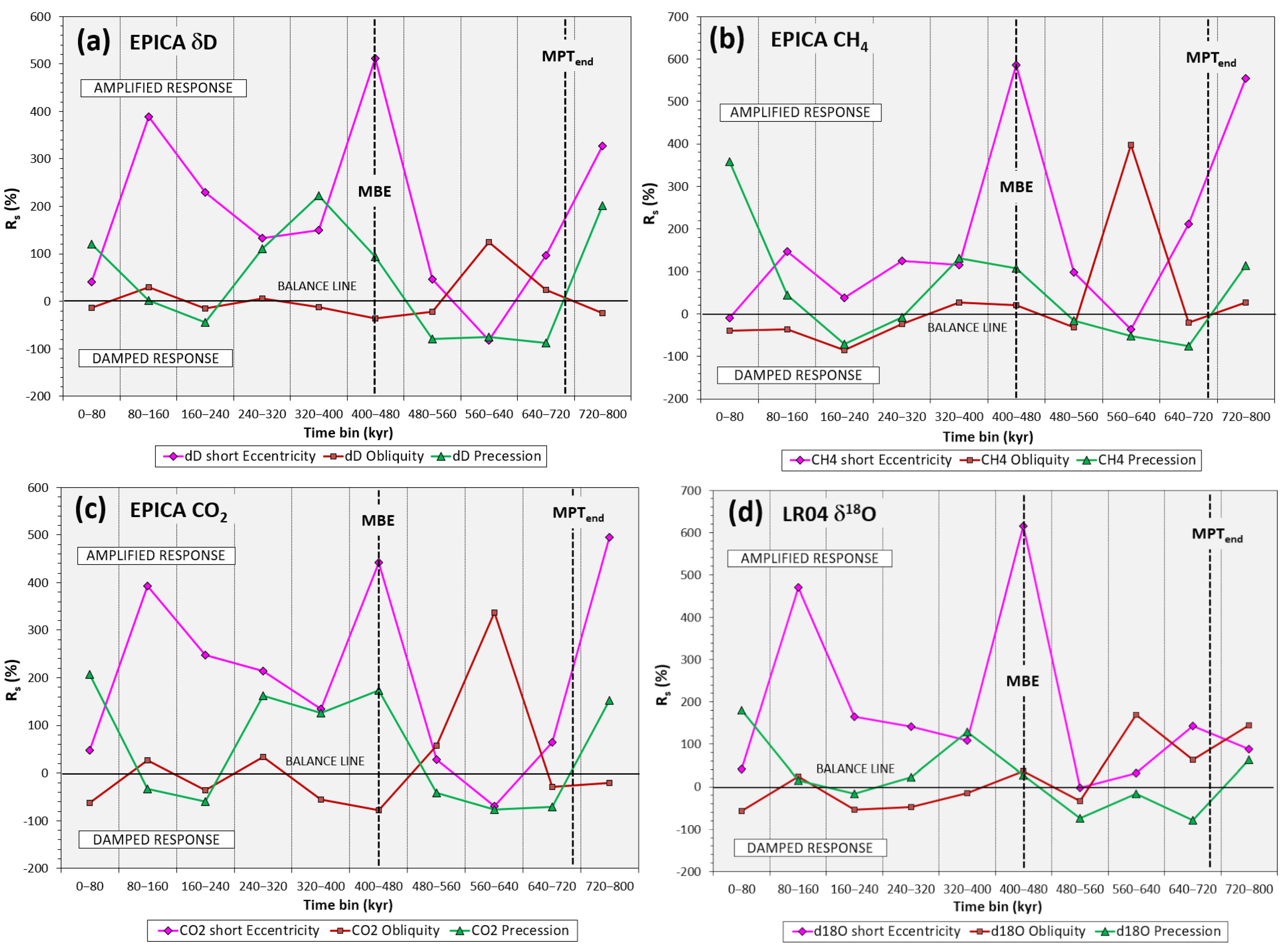
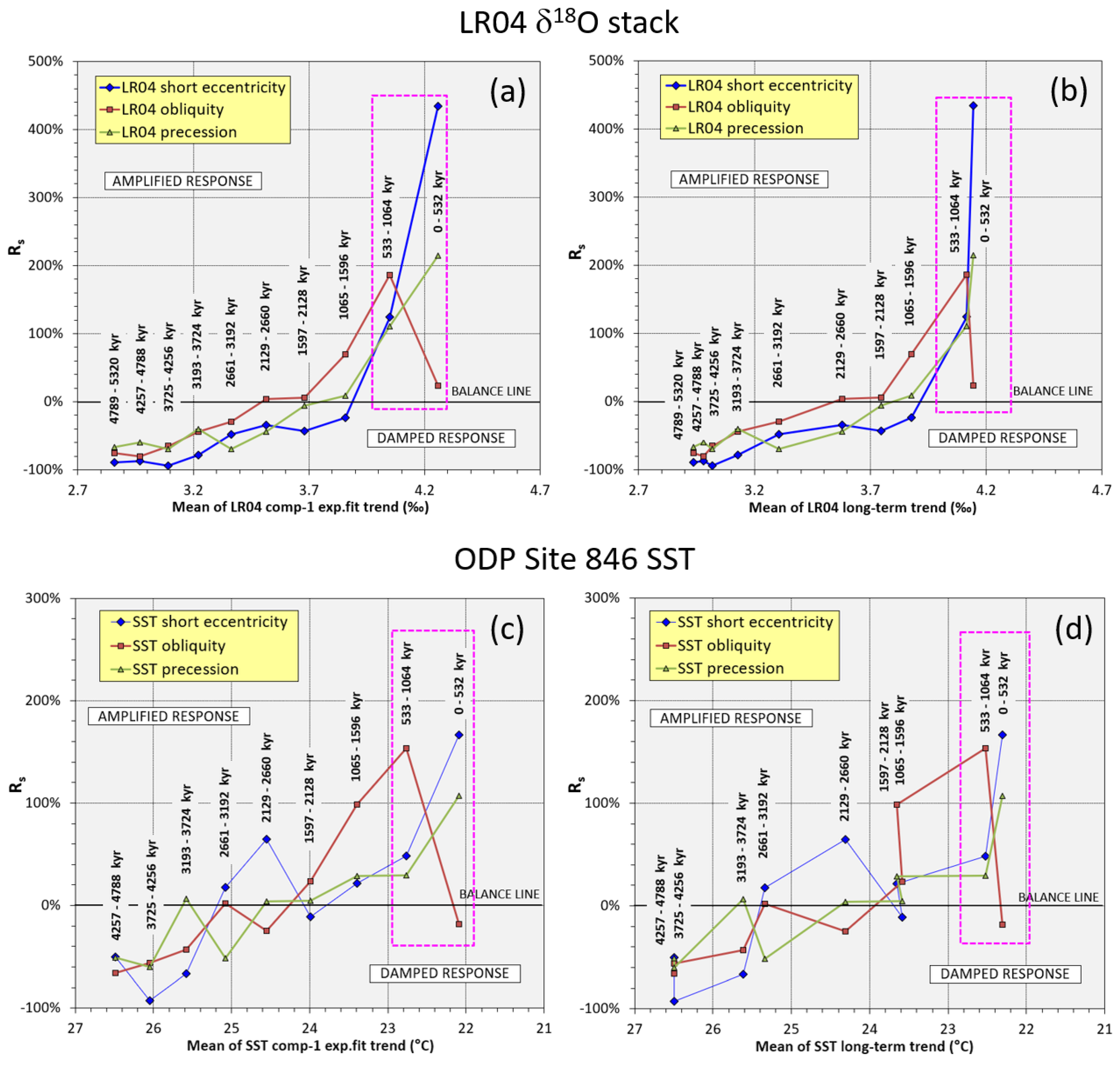
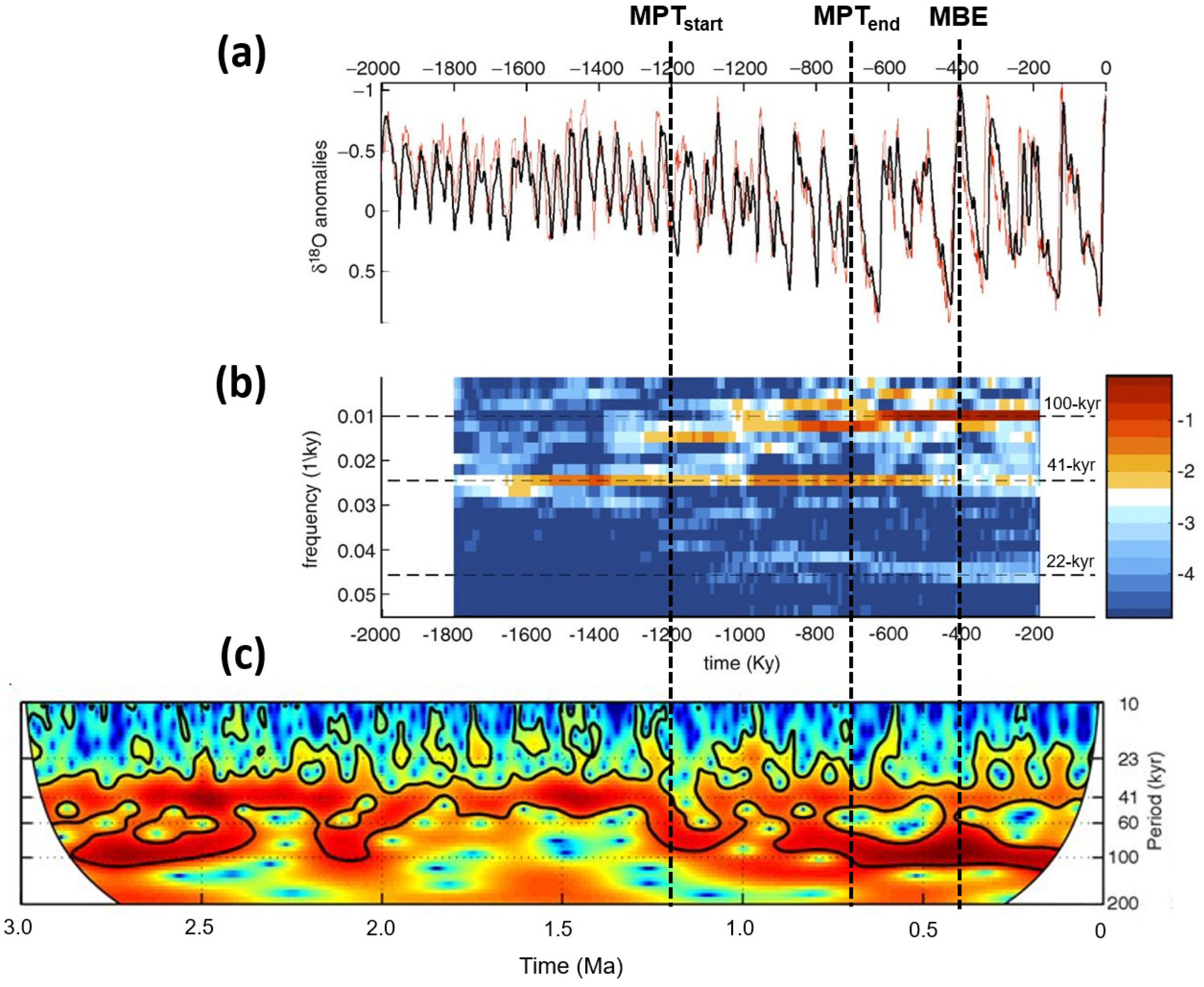
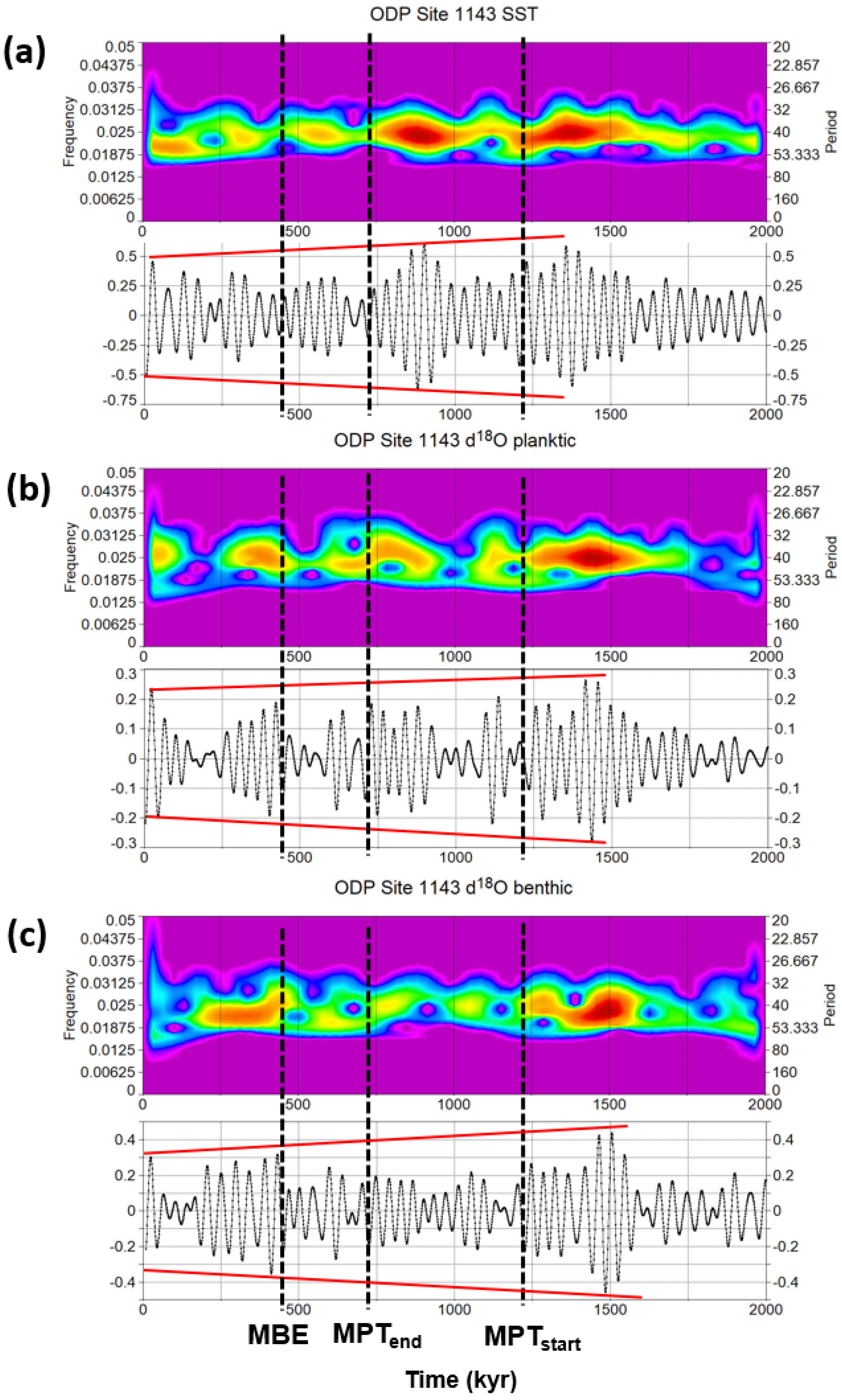
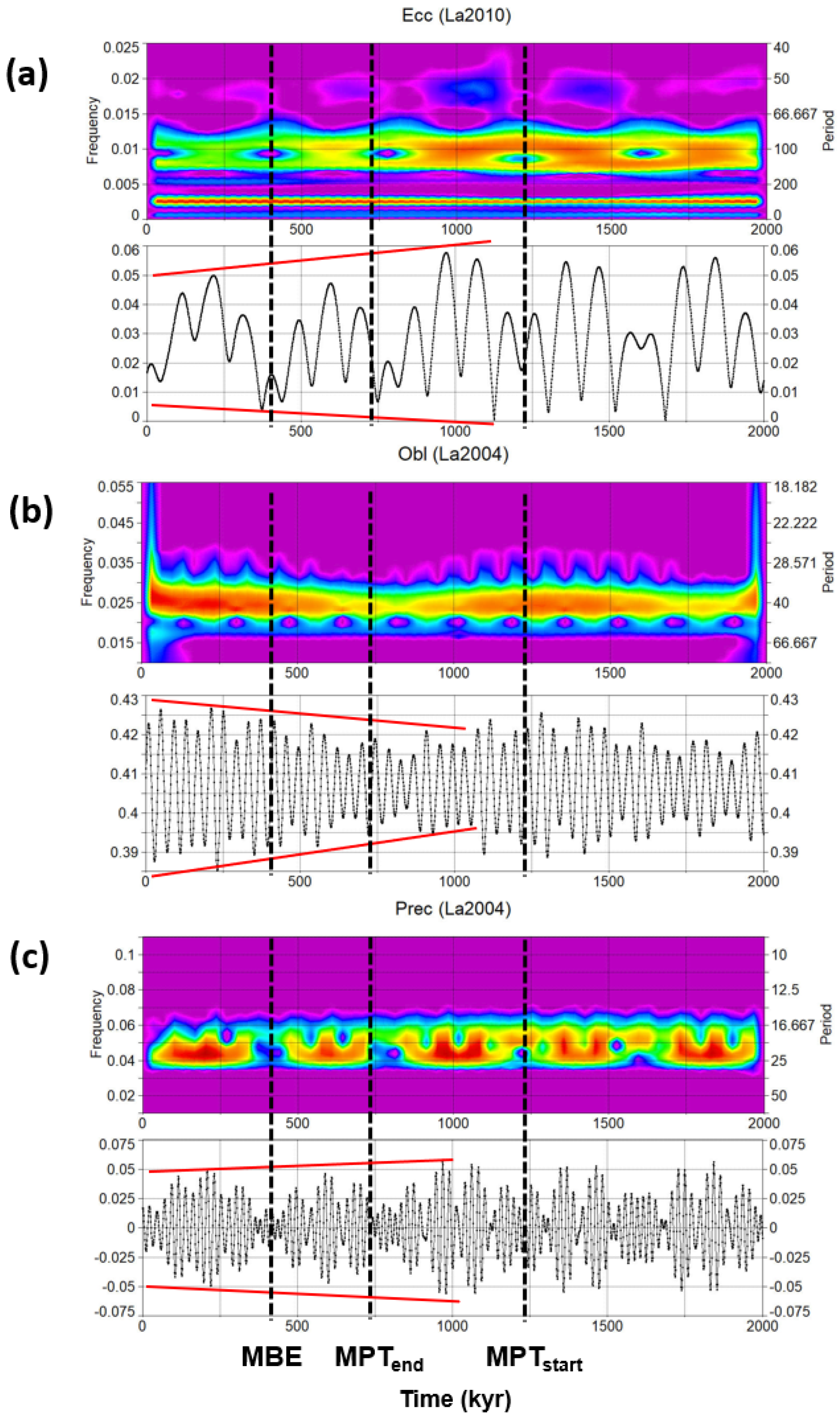
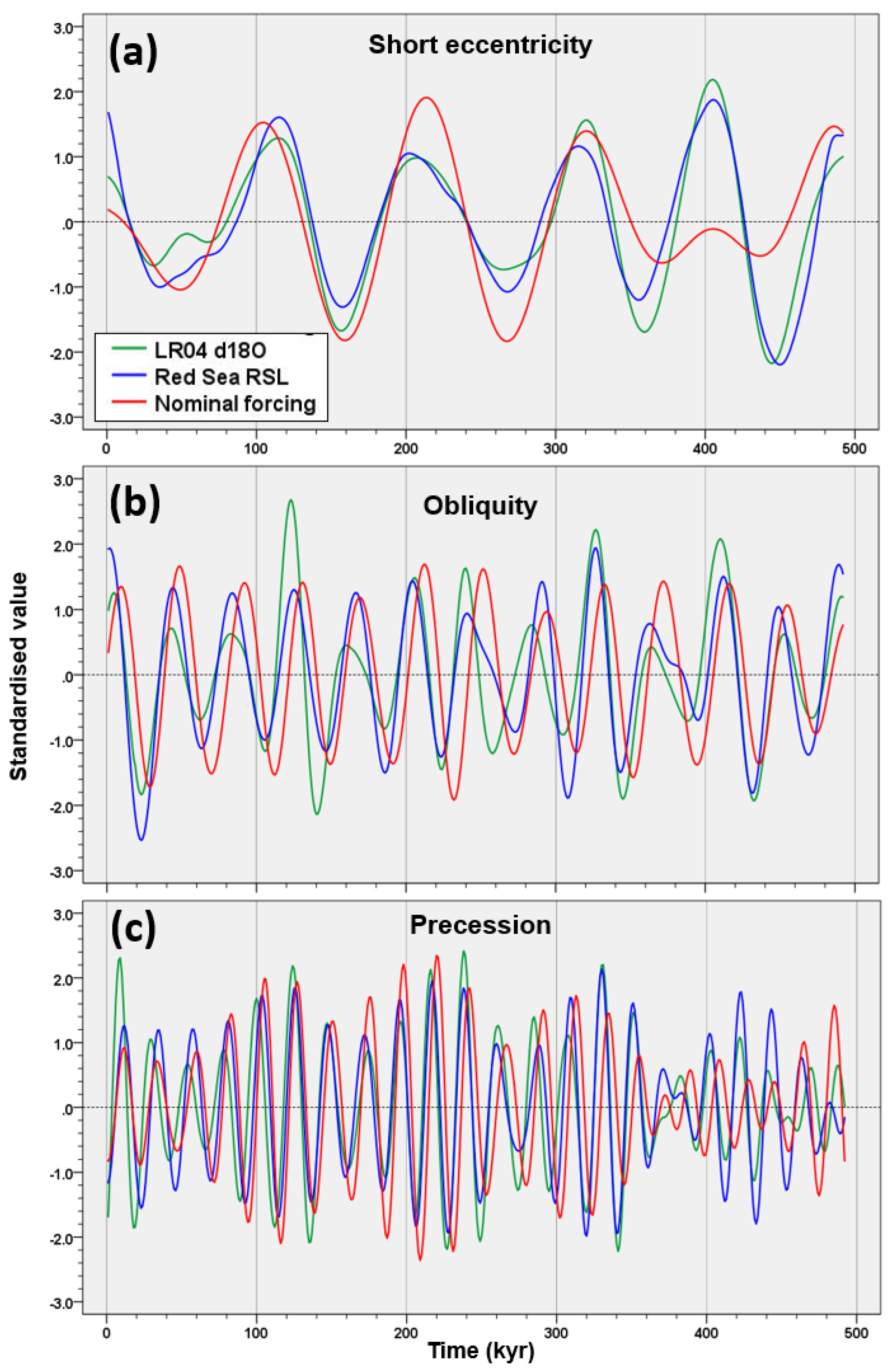
3.1. Evidence of Post-MPT Obliquity Damping

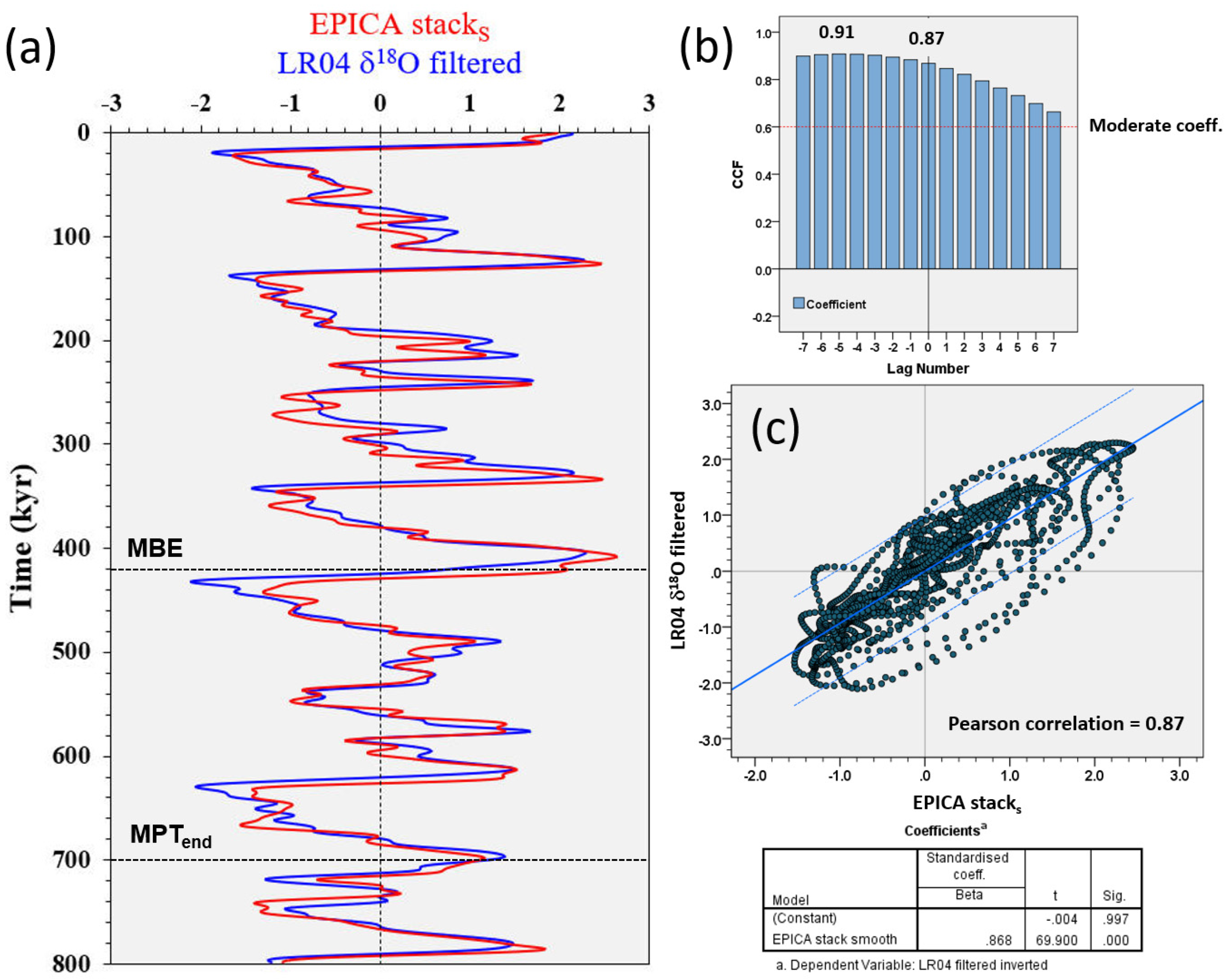
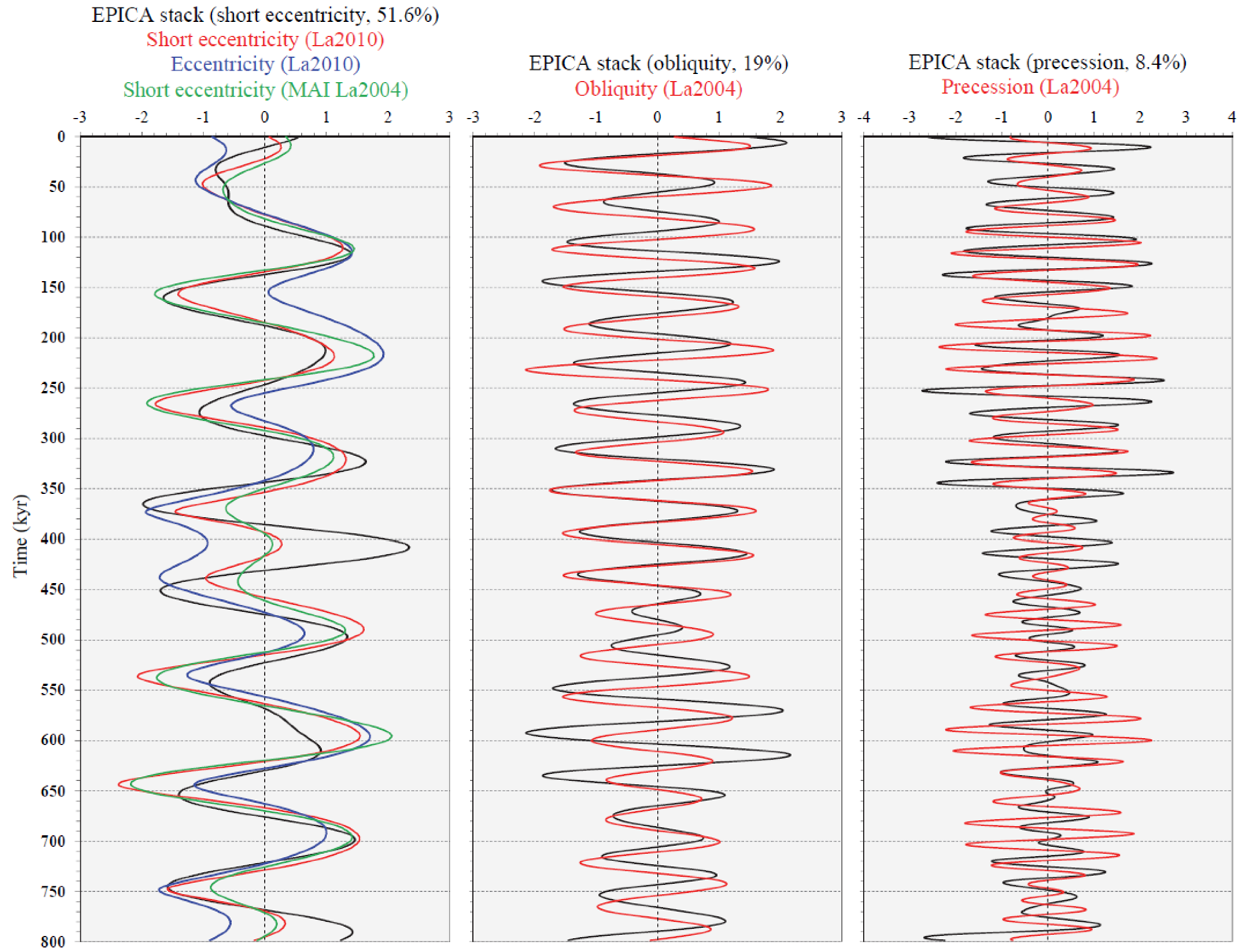
3.1.1. EPICA Record

R_s to orbital forcing—Quantitative analysis of the R_s to orbital forcings is demonstrated based on EPICA δD, CO₂, CH₄, and LR04 δ¹⁸O records for the last 800,000 years. Although the length of the current EPICA time series does not capture the complete temporal evolution of the MPT, some interesting features can still be observed. Viaggi [8] reported a sharp decrease in global δ¹⁸O and equatorial SST to near-zero values in obliquity R_s after 533 kyr. A similar post-MPT feature is observed in all EPICA obliquity δD, CO₂, and CH₄ signals since the 560–640 kyr time bin (Figure 1).

In fact, the obliquity R_s exhibits a nonlinear amplification of δD by 125%, and it reaches values of ~340% and ~400% for CO₂ and CH₄, respectively, at the 560–640 kyr time bin. After this amplification episode, a sharp decline in generalised obliquity R_s to near-zero values (balance line) or up to −80%, −60% is evinced since 560 kyr. The obliquity amplification and damping effects are more significant in the CO₂ and CH₄ responses. Also, the δ¹⁸O obliquity R_s shows nonlinear amplification of up to 170%, followed by a decline to a near-zero value or to a −60%, −50% damped signal. The short eccentricity R_s exhibits a similar shape among signals with a dominantly strong nonlinear amplification pattern within the 720–800 kyr time bin and after 480 kyr. Indeed, the R_s in short eccentricity amplification reaches its maxima up to ~400%, 600% with an attenuation episode at the 560–640 kyr time bin, thereby reaching values of –40%, −80%, which correlates with the obliquity amplification maxima (Figure 1). Two amplification maxima in short eccentricity R_s may be highlighted at the 400–480 kyr (δD = 510%; CO₂ = 440%; CH₄ = 590%; δ¹⁸O = 620%) and 80–160 kyr time bin (δD = 390%; CO₂ = 390%; CH₄ = 150%; δ¹⁸O = 470%), the former being the highest expression of the climate response amplification. The precession R_s oscillates quite regularly between damped cycles until up to −90%, and amplified responses up to 100%, 200%.

In general, we observe an inverse correlation between the R_s of short eccentricity and obliquity. These results are in agreement with the notion of a more intense MISs after 450 kyr compared to those from 800 to 450 kyr, which is consistent with a transition between two distinct climate states [59,80,81]. The increase in amplitude of the 100 kyr climate cycles began ~430 kyr ago, and is known as the Mid-Brunhes Event (MBE) [82]. It occurred within the Mid-Brunhes Oscillation (MBO) of global δ¹⁸O [8] and EPICA δD, CO₂, and CH₄ records [26]. Indeed, the MBE corresponds to the maximum short eccentricity R_s amplification of the last 800 kyr. In summary, the analysis of the Antarctic R_s reveals that since 480 kyr, a strong amplification of the short eccentricity signals has occurred (up to ~400%, 600%) coupled with damping of obliquity responses (up to −80%, −60%).

Table 1. The maximum amplitude amplification (R_s max) and the maximum amplitude damping (R_s min) rate of change in the signals (EPICA δD, CO₂, CH₄, and LR04 δ¹⁸O) over the last 800 kyr, normalised in % for kyr by forcing (80 kyr bin). Note the marked asymmetry of the climate responses with extremely robust amplitude magnifications and moderate damping.

Rs statistic	Signal	Short Eccentricity	Obliquity	Precession
Max	δD	6.40	1.56	2.78
	CO2	6.18	4.21	2.58
	CH4	7.32	4.97	4.48
	δ18O	7.70	2.11	2.25
Min	δD	−1.02	−0.45	–1.10
	CO2	−0.88	−0.97	−0.96
	CH4	−0.46	−1.08	−0.96
	δ18O	−0.04	−0.70	−0.97

shows the maximum amplitude amplification (R_s max) and the maximum amplitude damping (R_s min) values of the signals during the last 800 kyr, normalised in % for kyr. Interestingly, the R_s data show a marked asymmetry of the climate responses with very robust amplitude magnifications and moderate damping, similar to that documented from global δ¹⁸O and equatorial Pacific SST signals [8].

Factor model of orbital R_s—A PCA model of EPICA R_s data was obtained to investigate certain correlation patterns that are recognisable from Figure 1. The model converges on principal component 1 (PC-1), explaining 43.8% of the total variance, whose loadings on δD, CO₂, CH₄, and δ¹⁸O R_s express a positive correlation with short eccentricity and precession (which reflects the eccentricity modulation of precession), and an anticorrelation with obliquity (Figure 2). It is interesting to note that PC-1 tends to exhibit a positive correlation with the mean of the δ¹⁸O exponential trend, supporting a link between orbitals R_s and the long-term ice volume [8].

In particular, Figure 2b exhibits the PC-1 regression factor score and the δ¹⁸O exponential trend varying according to time bins, which reflects the increasing tendency of the PC-1 factor score (i.e., short eccentricity/precession amplification vs. obliquity damping) together with the δ¹⁸O enrichment towards the Late Pleistocene (post-MPT). However, the most pronounced δ¹⁸O enrichment rate occurred earlier in subtrend IV, which includes the MPT [8], present work. The turning point (PC-1 = 0) between the mean values of negative (high obliquity R_s vs. low short eccentricity R_s) and positive (low obliquity R_s vs. high short eccentricity R_s) PC-1 is within the time range 560–400 kyr (Figure 2b), marking the transition to MBE at ~430 kyr. These results suggest that PC-1 is a latent factor underpinned by a post-MPT anticorrelation among obliquity and short eccentricity/precession R_s, which is related to the long-term growth of the cryosphere volume.

Rescaled quantitative impact—Viaggi [26] estimated the quantitative impact (% variance) of orbital and millennial-scale suborbital components using EPICA δD, CO₂, and CH₄ records for the last 800,000 years. The signal strength obtained by variance is a relative concept, and is inversely proportional to the total variance of the record being investigated, and thus to its temporal extension. Therefore, for a short time series, the same component exhibits more relevant strength compared to long time series because of the former ‘defect’ in total variance owing to the lack of high-order cycles or long-term trend [26]. In the present paper, the EPICA stack data were rescaled for the Plio–Pleistocene LR04 δ¹⁸O/SST orbital/suborbital variance [8] to provide a rough estimate on a long time frame and compare the results. Because the extremely small fraction of δ¹⁸O (0.5%) and SST (0.4%) ‘noise’ components of Viaggi [8] partly includes suborbital signals below the Nyquist’s condition, this fraction was included in the mean calculation base of 23.6% for rescaling EPICA stack signals. As expected in a post-MPT record, we observed that the short eccentricity is primarily responsible for the variance in the EPICA components, which was estimated to have a stack mean of 51.6% [36]. This relevant strength of the short eccentricity signal reflects the robust nonlinear amplification pattern shown by R_s analysis (Figure 1 and Figure 2). By rescaling this value on the Plio–Pleistocene variance, we obtain an estimate of 12.2%, which is very high compared to the global δ¹⁸O of 6.5% [8]. This difference should be apparent because the EPICA short eccentricity response is a post-MPT strong amplified signal, whereas the Plio–Pleistocene LR04 δ¹⁸O contains a long pre-MPT record of weak eccentricity response [7,8,25]. The EPICA obliquity band accounts for a stack mean variance of 19.0%, which is almost equivalent to a Plio–Pleistocene rescaled variance of 4.5%. As opposed to the short eccentricity, this value is clearly too low compared to the LR04 δ¹⁸O value of 9.9%. This may be because of the dominance of the damped signal in the EPICA post-MPT obliquity record, which is in agreement with the R_s analysis, whereas the δ¹⁸O includes a long pre-MPT record of strong obliquity response [25]. The EPICA stack mean variance driven by precession can be estimated to be 8.4%. On the Plio–Pleistocene rescaled variance, the Antarctic precession stack corresponds to 2.0%, which is close to the global δ¹⁸O value of 2.0% because even the LR04 precession signal exhibits an amplitude increase during MPT and post-MPT times [8,25].

Wavelet power spectra and SSA signal structural observations—Figure 3 shows the Morlet wavelet power spectra of EPICA short eccentricity, obliquity, and precession SSA stacks [26]. We observed a decrease in the obliquity response after ~550 kyr associated with an evident increase in both short eccentricity and precession power.

An Antarctic SSA signal structural observation related to the eccentricity–obliquity link can be seen in Figure 4. δD, CO₂, and CH₄ component-2 signals exhibit two or three low-amplitude 41 kyr obliquity peaks (glacial/interglacial) embedded in a weak ~93/75 kyr framework [26]. In contrast, the obliquity maxima associated with glacial terminations appear more pronounced. These features are similar to the shapes shown by Viaggi [8] for the global δ¹⁸O and equatorial SST components 3–4 during the MPT, and may be further evidence of an obliquity attenuation phenomenon. This suggests a connection between short eccentricity and obliquity, a possible observational reminiscent of the ‘obliquity-cycle skipping’ model [21,22].

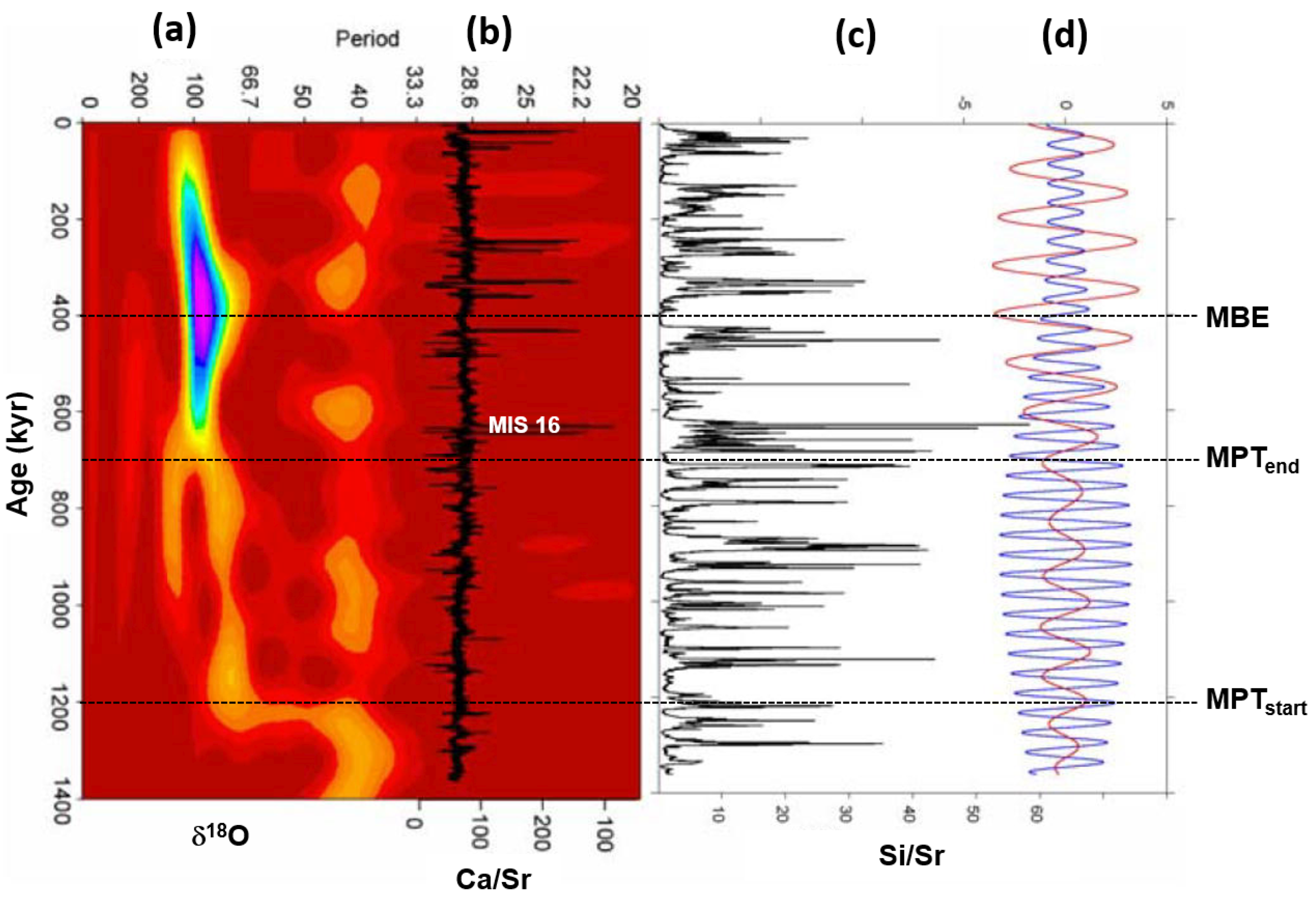
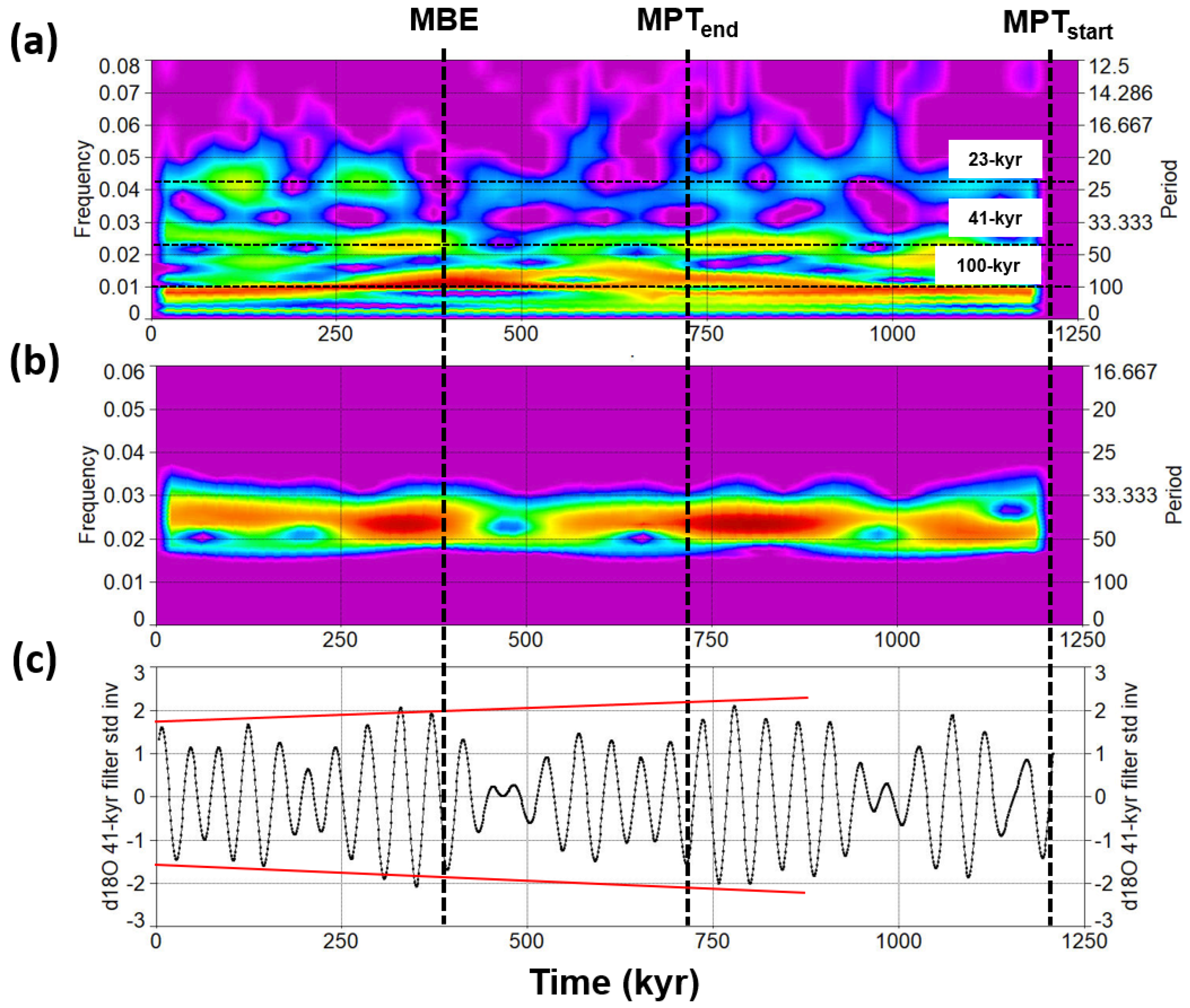
3.1.2. Sea-Level Record of the Red Sea

Fourteen SSA orbital components were identified in the present work from the RSL record of the Red Sea [71]. The components spanned from short eccentricity to precession, and they cumulatively explain 86.1% of the original variance (

Table 2. Results of quantitative estimation of the signal magnitude (percentage variance) and Fourier frequency data of the three Red Sea RSL reconstructed components isolated by singular spectrum analysis. The frequency peaks are the most significant peaks above a 99.9% critical limit. Original data are from Grant et al. [71].

RSL Component Rank	RSL Component Variance	Frequency (kyr−1)	TISA Power (%)	Period (kyr)	Forcing
1–2; 7–10	61.4%	0.01001973	100.0	100	Short eccentricity
3–4; 13–14	13.1%	0.02460637	84.8	41	Obliquity
		0.03244360	15.2	31
5–6; 11–12	11.7%	0.04393214	80.9	23	Precession
		0.05342083	19.1	19
15–200	13.8%				Suborbital + noise

). The reconstructed component of 100 kyr short eccentricity (comp-1–2; 7–10) explains 61.4% of the variance. The 41–31 kyr obliquity component (comp-3–4; 13–14) describes 13.1% of variance, followed by 11.7% of the 23–19 kyr precession signal (comp-5–6; 11–12). The strength of these orbital RSL signals for the last 500 kyr is very similar to the corresponding bands of the EPICA records for the last 800 kyr [36].

As in the case of EPICA, the RSL data were rescaled with respect to the Plio–Pleistocene variance to provide a rough estimate on a long time frame and compare the results (calculation base of 23.6%), which were found to be largely similar to those of EPICA (

Table 3. Comparison among the Red Sea RSL and EPICA Pliocene–Pleistocene rescaled variance vs. the LR04 δ¹⁸O. Δσ is the difference in variance between the RSL/EPICA and δ¹⁸O. Variance estimates are in terms of LR04 [8] and EPICA [26]. Original RSL data are from Grant et al. [71].

Forcing	Red Sea 1		Antarctica 1		LR04
	RSL (%)	Δσ (%)	EPICA (%)	Δσ (%)	δ18O (%)
Short eccentricity	14.5	8.0	12.2	5.7	6.5
Obliquity	3.1	−6.8	4.5	−5.4	9.9
Precession	2.8	0.8	2.0	0.0	2.0

¹ Rescaled variance.

). Indeed, as expected in a post-MPT record, the RSL short eccentricity is primarily responsible for the variance in the Red Sea record, being rescaled to 14.5%. Again, this strength is very high compared to the global δ¹⁸O of 6.5% [8]. The RSL obliquity signal is approximately equivalent to a Plio–Pleistocene rescaled variance of 3.1%. In contrast to the short eccentricity, this value is clearly too low compared to the LR04 δ¹⁸O of 9.9%, corroborating the RSL obliquity damping evidence, similar to the EPICA record. The Red Sea RSL precession signal corresponds to 2.8% rescaled variance, which is slightly amplified compared to δ¹⁸O.

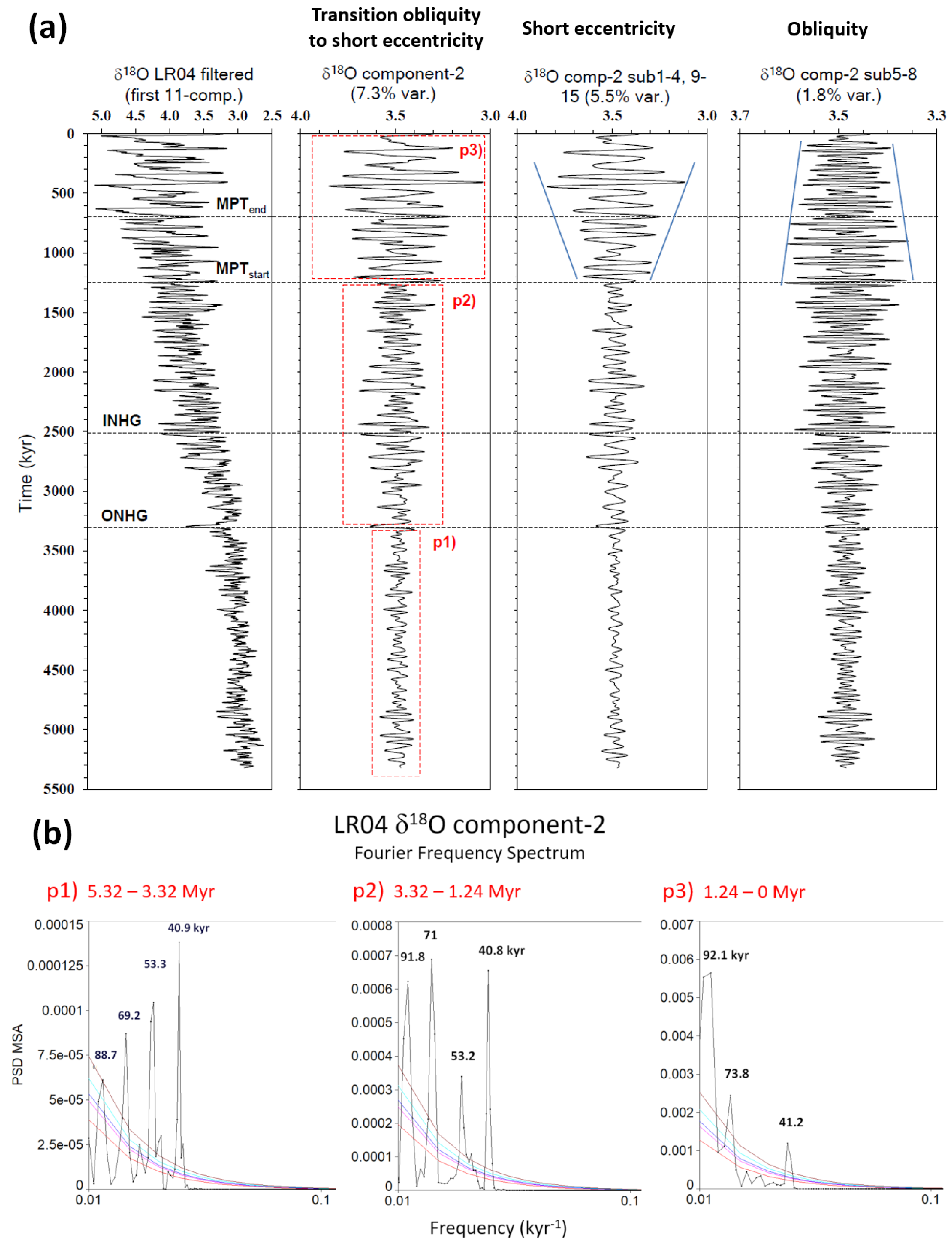
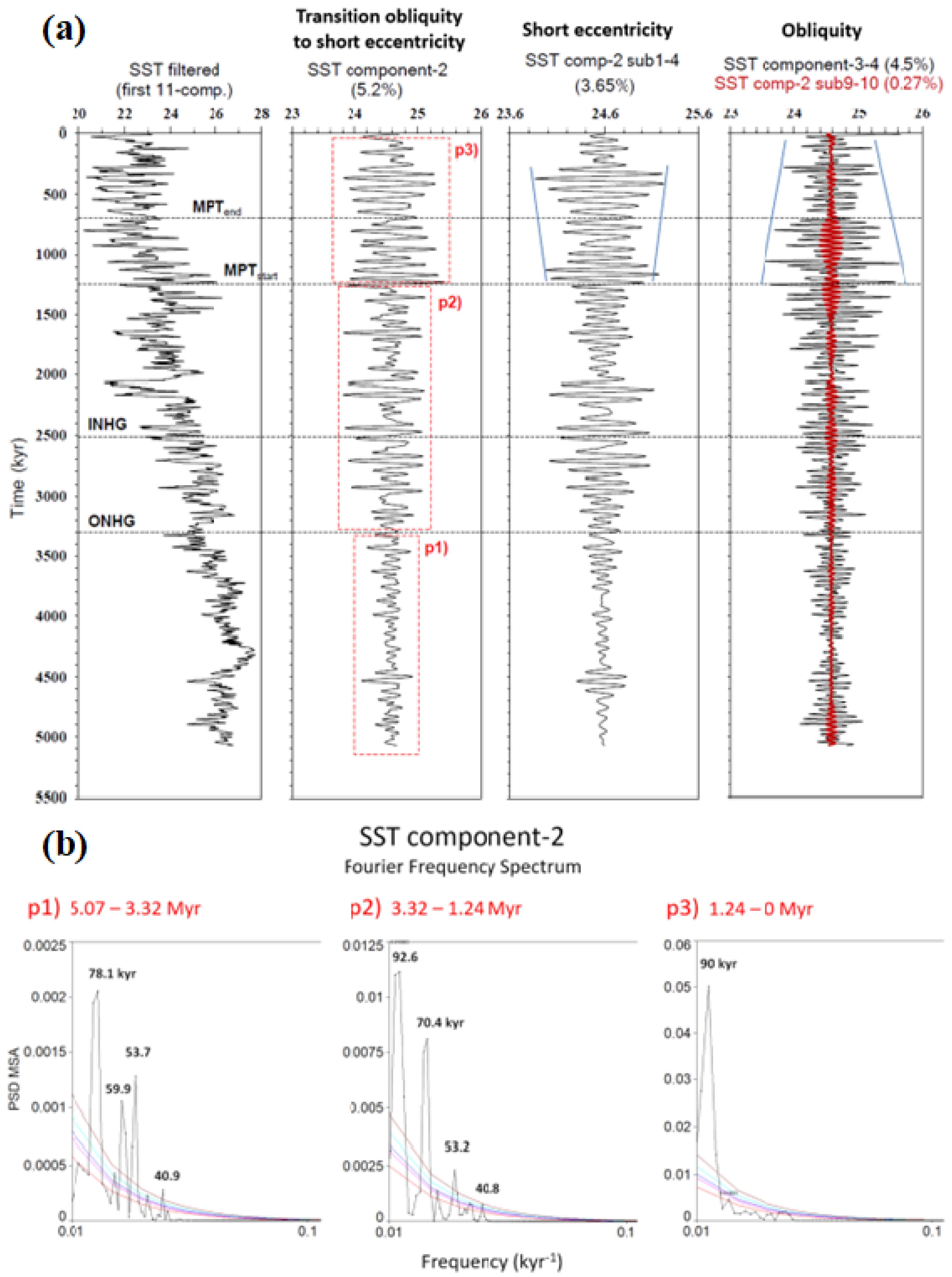
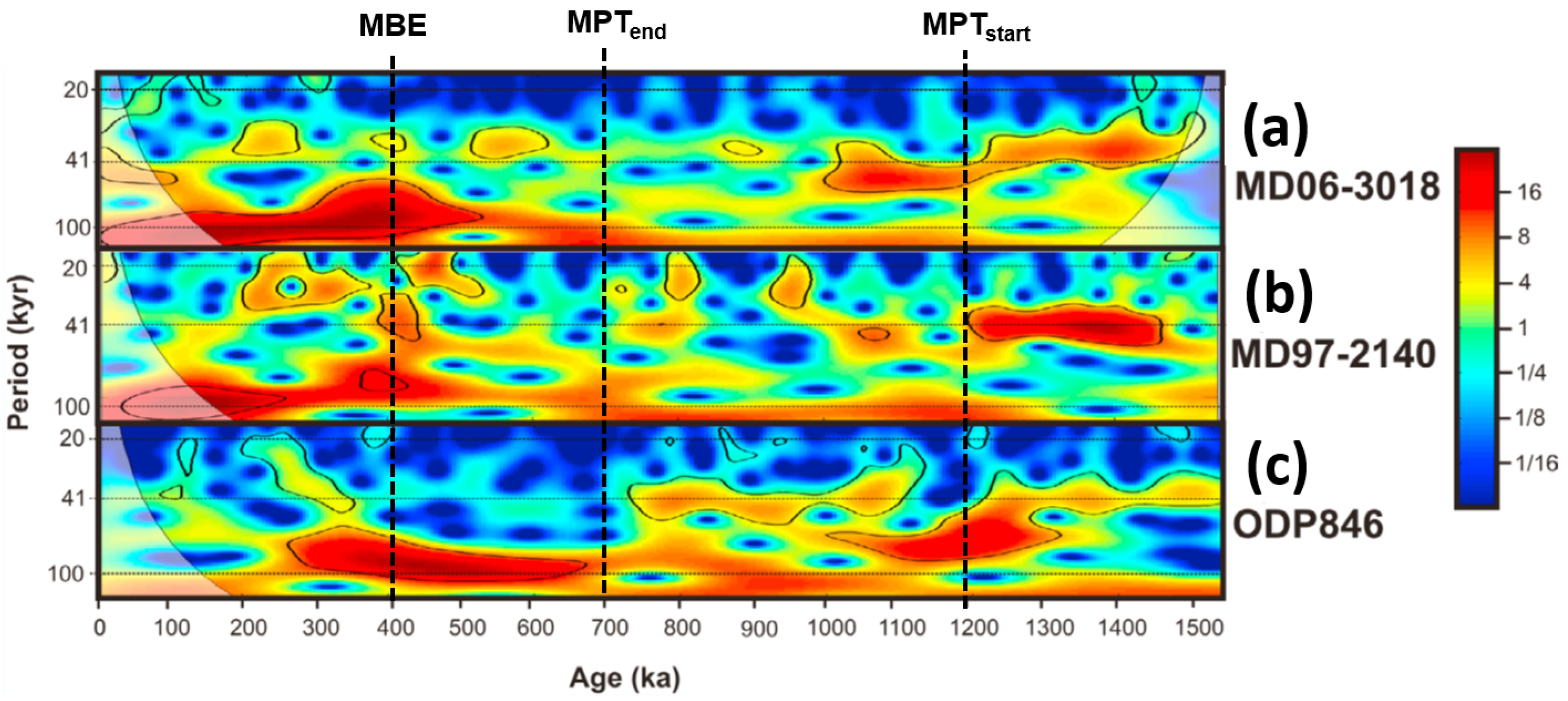
3.1.3. LR04 δ¹⁸O and Equatorial ODP Site 846 SST

R_s analysis—A remarkable indication of inverse coupling between obliquity damping and short eccentricity/precession amplification during post-MPT time is observed from LR04 δ¹⁸O and Site 846 SST records [8]. In this section, these observations are further developed. Figure 5 plots the Plio–Pleistocene orbital R_s (short eccentricity, obliquity, and precession) of global LR04 δ¹⁸O (a, b) and equatorial Site 846 SST (c, d) as a function of the long-term mean climate state (averages of exponential-fit trend and long-term SSA component expressing the climate background).

The values were calculated by arbitrary time segments binned at 532 kyr (data from Viaggi [8]). Reconstruction of orbital SSA components as follows (sub = subcomponent):

δ¹⁸O short eccentricity = (detrend comp-1 sub-3–11 × 0.95 + comp-2 sub-1–4; 9–15 × 5.5)/6.45;

δ¹⁸O obliquity = (comp-3–4 × 8.1 + comp-2 sub-5–8 × 1.8)/9.9;

δ¹⁸O precession = comp-5–7;

δ¹⁸O lomg-term trend = comp-1 sub-1;

SST short eccentricity = (comp-2 sub-1–4 × 3.65 + comp-2 sub-5–8; 11–15 × 0.5 + detr comp-1 sub-3–11 × 0.93) / 5.08;

SST obliquity = (comp-3–4 × 4.5 + comp-2 sub-9–10 × 0.27 + comp-2 sub-5–8; 11–15 × 0.76)/5.53;

SST precession = comp-5–7;

SST lomg-term trend = comp-1 sub-1).

R_s was calculated with respect to nominal forcing (eccentricity La2010, [38]; obliquity and precession La2004, [37]. Figure 5a,b exhibit a δ¹⁸O nonlinear amplification of the short eccentricity R_s up to ~440% towards the Mid-Late Pleistocene, similar in shape with that of the precession response but with a magnitude of up to ~200%. The δ¹⁸O obliquity R_s shows a nonlinear amplification of up to 180% towards the end of the MPT, followed by a strong depletion in variance to a near-zero value at post-MPT (0–532 kyr bin). This R_s pattern is similar to the regional equatorial SST record (Figure 5c,d), although the values are more scattered with a smaller positive magnitude of short eccentricity (it does not reach 200%) and precession amplification of up to ~100%. The SST obliquity R_s also shows strong variance depletion of up to −20% post-MPT.

R_s orbital factor model—A PCA factor model was obtained to investigate the correlation patterns recognisable from Figure 5 by integrating the temporal R_s data of both δ¹⁸O and SST records with the long-term mean climate state (Figure 6). For this Plio–Pleistocene dataset, the model solution identified two principal components that explain 94.6% of the total variance. PC-1 (57.7%) (Figure 6a) exhibits a strong positive loading on both δ¹⁸O and SST short eccentricity/precession R_s, which is strictly related to the long-term δ¹⁸O enrichment and long-term SST depletion. PC-2 (36.9%) (Figure 6b) shows robust positive loadings on both δ¹⁸O and SST obliquity R_s, which are related to the long-term δ¹⁸O enrichment/SST depletion.

It is worth noting that these Plio–Pleistocene factors (Figure 6c) corroborate the latent link between the increasing amplitude of all orbital climate responses and the anticorrelation between obliquity and short eccentricity with the progressive development of the Earth’s icy state [8], which is in agreement with the factor model of EPICA. In detail, as shown in Figure 6d, the spread of PC factor scores (namely the difference PC-2–PC-1) highlights the post-MPT anomalous depletion of the obliquity’s R_s which appears as the strongest final stage of similar and less marked PCs anticorrelation patterns since ONHG and INHG events (red bar). Indeed, the absolute factor spread exhibits two patterns of increasing value and inverse coupling (anticorrelation) among climate responses to forcings through time. They include a positive spread (blue bar), showing high obliquity associated to low short eccentricity/precession R_s, and negative spread (red bar), showing low obliquity linked to high short eccentricity/precession R_s. These response configurations are associated with three transition patterns of positive to negative spreads, including ONHG (Transition-1, TRA-1), INHG (Transition-2, TRA-2), and MBE (Transition-3, TRA-3), the latter being characterised by a high magnitude and incorporation of the MPT. Thus, the strengthening of the short eccentricity signal appears to be associated with the obliquity-damped response, whose maximum expression is observed in post-MPT, and is preceded by an earlier and weaker expression straddling the ONHG and INHG. These novel results suggest the traditional notion of the MPT to be the final, nonlinear transitional stage of a complex competing interaction between obliquity and short eccentricity forcing. It occurred under the influence of the long-term cooling that was already started during the Piacenzian (3.60–2.58 Ma), when the first weak spectral patterns of short eccentricity response are observed [8,83] and present work. This early evidence of short eccentricity response is sometimes known as the ‘premature 100-kyr cycle’ [84] or ‘early onset of the 100 kyr-like cycle’ [22]; however, it is referred by an accelerated cooling of SSTs from 1.2 to 0.9–0.6 Ma, which roughly coincides only with subtrend IV [8] and MPT.

In summary, the R_s analysis documented by EPICA δD-CO₂-CH₄, global δ¹⁸O, and equatorial Pacific SST records supports the orbital climate responses as being interpreted as predominant nonlinear feedback signals, paced by orbitals [7,21,24,72,85] and damped or amplified asymmetrically in a range from −100% to +400%, +600% the forcing (i.e., as a stacked signal among the primary perturbation of the forcing and the related feedback responses), depending on the long-term mean climate state and cycle periodicity [8,26,86]. The nonlinearity is linked to the scale-dependent net balance of positive and negative feedback processes associated with carbon/water cycles and albedo mechanisms (e.g., ice albedo, dust albedo, vegetation albedo) under the influence of variable initial conditions [4,7,8,10,12,24,26,27,31,40,66,87,88,89,90,91,92,93,94]. In other words, orbitals pace the frequency beat of the climate response and the feedback mechanisms nonlinearly transfer most of the system energy, with the least powerful climate mitigation processes. This implies that the natural climate system is dominated by positive feedbacks capable of making extremely strong amplification with responses of up to five to seven times the forcing. This leads to the exponential behaviour of the climate system (see Figure 10 in [8]), which has crucial quantitative implications also for present day climate change [95,96]. This interpretation may explain the energy excess ‘paradox’ of the astronomically paced signals compared to the small energy of orbital forcing, especially with respect to the eccentricity bands [2,4,10,97,98,99]. Indeed, the maximum Plio–Pleistocene exponential growth of the LR04 δ¹⁸O short eccentricity variance (e^2.93x) suggests an enhanced sensitivity of short eccentricity forcing to nonlinear amplifying feedback mechanisms on a long duration cycle during the Mid-Late Pleistocene icy state [8]. The δ¹⁸O exponential coefficient progressively decreases for short length cycles from obliquity (e^1.88x) to precession (e^1.78x) to half-precession (e^1.05x).

SSA—structural signal observations: An SSA structural evidence of the latent link between obliquity and short eccentricity comes from LR04 δ¹⁸O component-2 (transition obliquity to short eccentricity), where the transitional change in the nonlinear dynamic can be configured as a sort of ‘switching’ of the orbital power between the 41 kyr obliquity and 71/92 kyr eccentricity cycles [8] (Figure 7). In particular, the increasing amplitude of the short eccentricity subcomponent is coupled with an obliquity amplitude reduction during MPT and post-MPT time. Variations in amplitude are basically gradual, although nonlinear. Similar SSA features are also recorded in the equatorial Site 846 SST (Figure 8). The transition nature from obliquity to short eccentricity is less evinced in this SST record likely because of the low latitude of this site. The increasing amplitude of the short eccentricity is clearer in subcomponent-1–4. The decrease in the obliquity response is highly evident.

Further observations of the SSA structural signal for a special link between obliquity and short eccentricity come from Figure 9. Here, we can see a particular shape of the δ¹⁸O and SST component-3–4, where two or three low-amplitude 41 kyr obliquity peaks (glacial/interglacial) are embedded in a weak ~74/92 kyr framework. Similar to those shown in the EPICA records, these shapes seem reminiscent of the ‘obliquity-cycle skipping’ model [21] and corroborate the observations of Liu et al. [22].

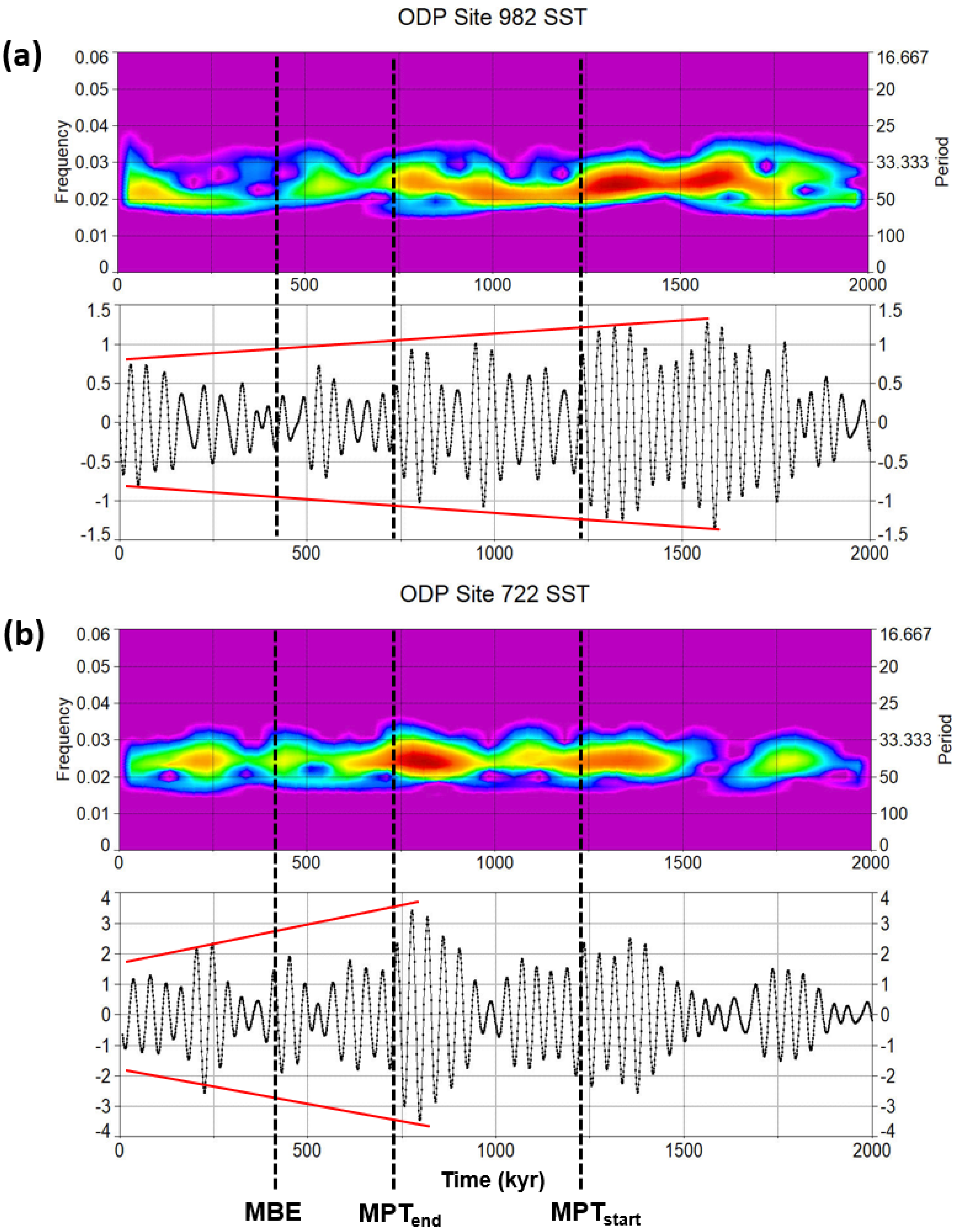
3.1.4. Atlantic, Pacific, Mediterranean, and Indian Proxies

New additional evidence of the coupling between obliquity damping and short eccentricity amplification is highlighted in Figure 10 at Site U1308 (eastern North Atlantic) from the work of Hodell et al. [62]. Here, the authors depict the 41 and 100 kyr filtered components of the Si/Sr signal, which show a clear decrease in obliquity amplitude coupled with an increase in short eccentricity amplitude during the MPT and post-MPT time (Figure 10d). The onset of IRD deposition enriched in detrital carbonate (Ca/Sr peaks) during the MIS-16 (Figure 10b) marks the reversal of the anticorrelation pattern between the obliquity and short eccentricity of the Si/Sr signal after the MPT_end (Figure 10d). Hodell et al. [62] speculate that the thickness of ice sheets and the duration surpassed the critical threshold during MIS-16 and activated the dynamical processes responsible for Laurentide ice-sheet instability in the Hudson Strait region. It should be noted that MIS-16 is at the top of the global δ¹⁸O subtrend IV, indicating that the largest ice volume was reached by the Plio–Pleistocene long-term trend of the ice-sheet growth [8].

Hodell et al. [63] generated a continuous time series of Ca/Ti over the past 1.4 Ma, which reflect relative changes in biogenic carbonate and detrital sediment at Site U1385 (Shackleton Site) on the SW Iberian Margin (Figure 11). It is worth noting that, on this site as well, the orbital bandpass filters show the distinctive inverse amplitude coupling between obliquity and short eccentricity/precession components.

Lisiecki and Raymo [25] have reported that the change in δ¹⁸O glacial dynamics at ~1.4 Ma is associated with an abrupt decline in the 41 kyr power and a decrease in modulation sensitivity to obliquity. Moreover, Lisiecki [49] found that the obliquity power of the middle deep Atlantic (2300–4010 m) benthic δ¹³C decreased by 50% at 0.6 Ma, indicating a restricted change in obliquity-driven overturning circulation. This is concurrent with a dramatic increase in the 100 kyr power of benthic LR04 δ¹⁸O. Thus, MPT likely contributed to a ∼50% decrease in the obliquity power coupled to a 100 kyr power of relevant increase in the middle deep Atlantic δ¹³C [49].

Figure 12 shows the global δ¹⁸O glacial variability over the last 2 Ma in two different multi-site stacks, i.e., benthic–planktic δ¹⁸O [21] and benthic δ¹⁸O [39]. Figure 12b exhibits a strong post-MPT increase in 100 kyr (and more moderate 22 kyr) spectral power coupled to a relevant decrease in 41 kyr power, as evinced from the benthic–planktic δ¹⁸O stack [21]. These spectral features are similar to those of the LR04 record (Figure 12c) estimated from the work of Imbrie et al. [13].

The reconstructions of subtropical southwest Pacific climate variability over the Pleistocene were derived by Russon et al. [66] from coupled planktic foraminiferal δ¹⁸O-Mg/Ca measurements acquired from a southern Coral Sea sediment core at site MD06-3018 (Figure 13). A clear shift from ~40 kyr to ~100 kyr modes of reconstructed glacial–interglacial SST variability was observed over the MPT when compared with those of the sites MD97-2140 (western equatorial Pacific) and ODP 846 (eastern equatorial Pacific). The wavelet power spectra in these sites again highlight the same relationship between SST obliquity-damped responses and the coupled increase in short eccentricity power.

Konijnendijk et al. [70] provided a ~1.2 Ma long benthic δ¹⁸O record from the eastern Mediterranean based on ODP Sites 967/968. Figure 14a exhibits the wavelet power spectra of the δ¹⁸O data provided by Konijnendijk et al. [70] and Figure 14b,c show the power spectra and time series of the wavelet filter centred on the 41 kyr cycle. Although it is less evident in the Mediterranean site, there is a slight reduction in the power/amplitude of δ¹⁸O obliquity, associated with an increase in power at both responses of short eccentricity (strong) and precession.

Lawrence et al. [64] provided the first continuous, orbital-resolution SST record from the North Atlantic ODP Site 982 that is located on the Rockall plateau, which is a critical region for understanding the origin of the Plio–Pleistocene ice ages because of its high sensitivity to changes in North Atlantic atmospheric pressure systems and North Atlantic drift. This site is particularly interesting because it exhibits high-amplitude variations derived from unusual obliquity [64]. Figure 15a shows the wavelet power spectra of the SST 41 kyr filtered component from the 1 kyr resampled data of Site 982. The plot demonstrates a relevant decrease in the 41 kyr spectral power and signal amplitude during MPT and post-MPT. Herbert et al. [40] published the estimates of SST at four tropical sites on the basis of alkenone paleotemperature determinations. They interpreted the similarity of tropical SST changes, in dynamically dissimilar regions, to reflect ‘top-down’ forcing through atmosphere circulation and strong GHGs feedback amplification, which connects the fate of northern hemisphere ice sheets with global ocean temperatures. More significantly, Figure 15b exhibits the SST obliquity damping feature by wavelet filtering and power spectra from the ODP Site 722 located in the Arabian Sea, Indian Ocean [40].

ODP Site 1143 is located within a basin on the southern continental margin of the South China Sea (tropical western Pacific). It provides planktonic δ¹⁸O [67], benthic δ¹⁸O [68], and SST [69] records covering the last 4 Ma. Figure 16 shows the wavelet power spectra of the 41 kyr filtered components over the last 2 Ma from the 1 kyr resampled data of Site 1143. A significant decrease in 41 kyr spectral power and signal amplitude is evinced during the MPT and post-MPT period.

Finally, it is very interesting to observe evidence of obliquity damping from the historical work of Hays et al. [72], which is based on composite records from Sites RC11-120 and E49-18 of the southern Indian Ocean (Figure 17). Here, the 40 kyr components of both planktic δ¹⁸O and SST records exhibit a clear damping trend in amplitude during the last 400 kyr.

These relevant observations from global and regional records (Antarctic, North Atlantic, Atlantic–Iberian margin, Mediterranean, western and eastern tropical Pacific, Pacific–South China Sea, Indian–Red Sea, Indian–Arabian Sea, southern Indian) of different climate-related proxies show that the coupling between obliquity damping and short eccentricity amplification is a widespread feature of the Mid-Late Pleistocene climate system, which could be the missing link in the MPT origin. There is a substantial variability in the intensity of obliquity damping at some single-site records (e.g., low intensity in Mediterranean Site 967/968) likely due to the different sensitivity to the obliquity of ocean basins and site locations (e.g., latitude, circulation). Understanding this phenomenon is crucial because the obliquity attenuation could have contributed to the strengthening of the short eccentricity response, favouring a long-lived feedback-amplified ice growth.

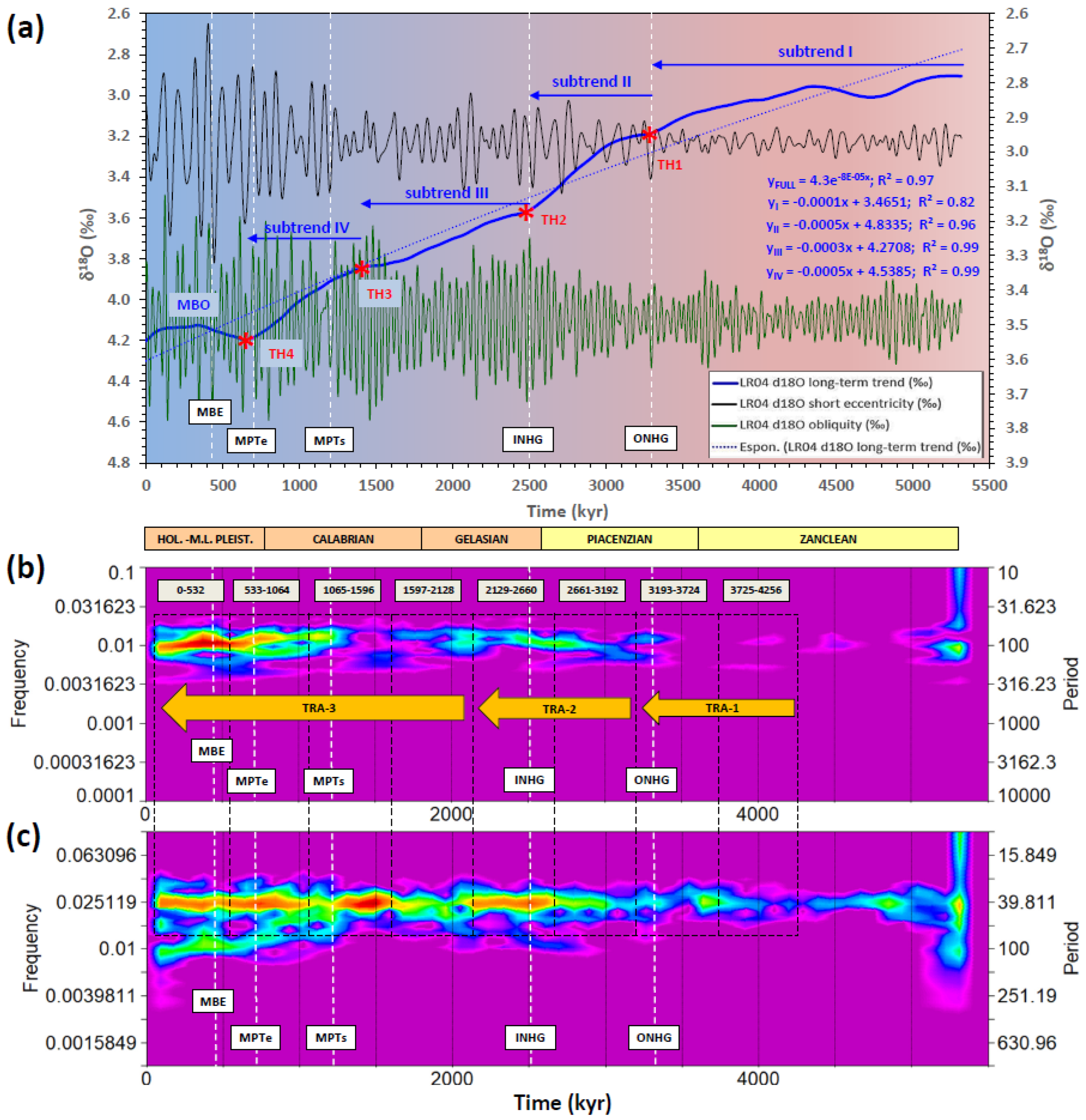
3.2. Long-Term Cooling Sets Boundary Conditions for Glacial/Interglacial Cycles

This section discusses the role of the long-term trend in the MPT debate in relation to the results highlighted above. Viaggi [8] investigated the records of the global LR04 δ¹⁸O stack [39], the equatorial ODP Site 846 SST [40], and the global ΔSST stack [100] using SSA. The study found similar trend components in all records, which explain ~76% of the Plio–Pleistocene variance and appear to be related to the long-term pCO₂ proxies [100,101,102,103]. Statistical analysis suggests that such long-term trends significantly modified the mean climate state with respect to orbitals through time [8], thereby hinting the background forcing to be relevant in setting boundary conditions for orbital climate responses [5,9,84,104]. This evidence of non-regional cooling trends is well supported by the work of McClymont et al. [84] on Pleistocene global SST records. The study showed that the variability of SSTs is superimposed upon a long-term cooling trend in oceanographic systems spanning the low to high latitudes and is accompanied by evolving pCO₂, abyssal ocean ventilation, atmospheric circulation, and/or dust inputs to the Southern Ocean. The ODP Site 982 (North Atlantic) and the ODP Site 1143 (southern South China Sea) both exhibit a remarkable trend of SST/δ¹⁸O cooling/enrichment over the last 4 Ma [64,69]. The close link between long-term cooling and the coupling between amplification of the short eccentricity and damping of the obliquity responses is corroborated by the results of the Plio–Pleistocene R_s orbital factor model shown in Figs. 5 and 6. The long-term cooling documented by the global LR04 δ¹⁸O stack is characterised by four step-wise subtrends [8], where terminal accelerations configure a mild curvilinear shape that is broken by slope changes representing four thresholds (TH1 to TH4) of mean climate state variation (Figure 18). The subtrend I occurs in the time interval of 5.33–3.30 Ma (Zanclean–Early Piacenzian) and culminates with the ONHG through a mild rate change of δ¹⁸O (linear equation Y_I). This subtrend is associated with the TRA-1 (Figure 6d), where the first weak response of the short eccentricity occurs straddling to the ONHG [8]. Subtrend II is Piacenzian in age, and exhibits the first strong acceleration of the changing rate, which terminates with the INHG (linear equation Y_II). It is followed by subtrend III with an intermediate rate of variation until up to 1.4 Ma (Gelasian–Calabrian p.p.). Subtrends II and III include TRA-2, where the second early manifestation and the more consistent short eccentricity response are observed across the INHG. The beginning of the MPT plots within subtrend IV (1.4–0.65 Ma) marks the second highest rate of change (linear equation Y_IV) during the Plio–Pleistocene long-term cooling trend and ice-volume growth. The end of the subtrend IV (MIS-16) indicates that the largest global ice volume was reached during the Cenozoic cooling [28,29], and marks the final stage of the MPT (~0.7 Ma). Interestingly, subtrend IV is associated with an accelerated rate of erosion/weathering cycles of the cratons surrounding the North Atlantic [105]. After MIS-16, the cooling trend was broken by a wide swing of global δ¹⁸O depletion and temperature recovery (SST, EPICA δD), which is characterised by a relative stasis of the ice growth and temperature cooling during the last 600 kyr (MBO). These are associated with a mild midterm GHGs recovery [8,26]. TRA-3, which includes MPT, occurs across subtrends III/IV and MBO, and shows the most relevant competing interaction between obliquity and short eccentricity responses under the influence of the long-term cooling (Figure 6). The strengthening of the short eccentricity signal appears to be associated to the obliquity-damped response (early manifestations across ONHG and INHG), whose maximum expression is observed during post-MPT (i.e., MBO time).

Although the proxy-based evidence for long-term cooling that is associated with an increased global ice volume appears to be reasonably credible, it is unclear how this background climate affected the MPT. Changes in diverse environmental parameters suggest that glacial climate boundary conditions evolved across the MPT and may have altered climate sensitivity to orbital forcing by placing pre-existing ice sheets closer to some threshold of the climate–ice sheet response [84]. Berger et al. [5] modelled the northern hemisphere ice-sheet volume to insolation forcing over the last 3 Ma. Under a warmer climate induced by higher atmospheric pCO₂, ice sheets never grow large enough during insolation minima such that they cannot survive any subsequent moderate insolation maxima, resulting in obliquity-related dominant cycles. Under cooler climate conditions, ice sheets survive through moderate insolation maxima and deglaciate entirely only under maximum insolation forcing (high eccentricity, high obliquity, boreal summer at the perihelion). Modelling results by Bintanja and van de Wal [9] suggest that the gradual emergence of the 100 kyr cycles can be attributed to the increased ability of the merged North American ice sheets to survive insolation maxima and reach a continental-scaled size. An important feature is the increased inability of the system to reach full interglacial levels at the timescales of obliquity and precession, particularly in North America, where continuing cooling enabled ice sheets to overcome insolation maxima at ever-greater volumes [9]. However, the larger the ice sheet grows and extends towards lower latitudes, the smaller the insolation required to make the mass balance negative [27]. The cooling of climate is expected to be analogous to increasing the threshold for ablation in the insolation integrated over the summer period (summer energy) [104]. Summer energy suggests that an ice sheet will be the most sensitive to obliquity when its ablation zone exists at high latitudes with a low insolation threshold (warm climate background). However, the model produces a mostly linear obliquity response, and fails to produce trends towards greater amplitude [104]. This is a common problem with models that fail to accurately reproduce the observed records [13,19,20].

The Plio–Pleistocene long-term cooling and the peculiar geographic setting of Greenland and North America have certainly led to more favourable boundary conditions for snow preservation at high latitudes. It is likely that the key role of the long-term cooling in MPT is to increase the scaling effect of feedback mechanisms in response to orbital forcing, thus resulting in an increase in the amplitude of climate responses as observed in Plio–Pleistocene proxies. However, the long-term cooling cannot explain alone the obliquity damping observations from climate proxies in the context of an increase in the obliquity nominal forcing during the Mid-Late Pleistocene, as shown in the next section.

3.3. Amplitude Relationships between Orbital Forcings and Proxies

A common feature of the anticorrelation among climate proxies is the unexpected obliquity power/amplitude reduction coupled with an increasing power/amplitude of the short eccentricity response because this characteristic is not found in the nominal solutions over the last 1.2 Ma [37,38] (Figure 19). In fact, the amplitude trends and the power spectra of the orbital solutions appear to have an inverse relationship with those of the related climate proxies: obliquity nominal increase vs. proxy-decrease and short eccentricity/precession nominal decrease vs. proxy increase. These relationships are reflected in R_s data ([8]; this study). On the other hand, there is no univocal relationship between the strength of the astronomical forcing and the intensity of the related climate response [59]. Although the power/amplitude of the climate response should be theoretically consistent with that of forcing, the amplification or damping in relation to the net balance of positive and negative feedback mechanisms, and the effect of the initial conditions, may alter this linear connection [7,8,9,10,24,26,31,89,91,93,94]. Since obliquity is a relevant forcing to high-latitude ‘ice killing’, it is difficult to understand what ordinary negative feedback mechanism might have dampened the climate response of obliquity in the context of an increasing amplitude of nominal forcing during the last 1.2 Ma.

In the following section, we have critically reviewed the theoretical constraints required by the ODH for obliquity–oblateness feedback relevant to the uncertainties in the obliquity phase lag estimates and oblateness changes.

3.4. Why the Dampening of the Obliquity Response?

A crucial characteristic of the damping of climate proxies in the obliquity band is its symmetry, which suggests attenuation of the forcing during both interglacial (high obliquity) and glacial (low obliquity) stages. In order for the ODH to achieve this bipolar damping by obliquity–oblateness feedback, it theoretically requires that a negative secular change occurs during the obliquity maxima (interglacial) and a positive change takes place during the obliquity minima (glacial), based on the model of [46] (Figure 20). Specifically, mandatory constraints are a low-obliquity lag response of the ice sheet (<44°; <5.0 kyr) and a positive (interglacial damping)/negative (glacial damping) changes in oblateness.

3.4.1. Remarks on Obliquity Phase Lag and Temperature/Ice-Volume Proxies

Response phase lags are difficult to estimate (e.g., age models) and should be compared within the same time interval with preferably evenly spaced records and the same spectral analysis parameters. Conceptually, the benthic δ¹⁸O measures changes in global ice volume and deep-water temperature, which are controlled by the high-latitude surface temperature [25,47]. δ¹⁸O changes are globally assumed to be synchronous within the mixing time of the ocean (~1 kyr) because the δ¹⁸O composition of foraminiferal tests is primarily controlled by the storage of ¹⁸O-depleted water in ice sheets [48]. However, few studies have revealed that diachronous changes in the deep-water temperature between Atlantic and Pacific basins produce significant lags in benthic δ¹⁸O [47,48,106]. Moreover, the benthic δ¹⁸O records from different depths in the same ocean might have experienced diachronous responses. Because the benthic δ¹⁸O signal is a composite of these two different processes, the net phase of the δ¹⁸O signal reflects the variable response time of the ice-volume and deep-water temperature components across ocean basins and site locations [40,47,48,66]. This may result in a lag bias in the benthic δ¹⁸O data, affecting phase shift estimates of the ice volume. To overcome this problem, other proxies may be considered to be not affected by deep-temperature bias, and the benthic δ¹⁸O deep-temperature bias may be estimated. The EPICA stack_s better approximate the global benthic δ¹⁸O signal (Figure 21), the latter being intrinsically related to the global/high-latitude surface temperature [25]. There is a striking similarity in the glacial–interglacial variability between EPICA stack_s and LR04 δ¹⁸O, even though amplitude offsets possibly exist resulting from the deep-temperature component of benthic δ¹⁸O and/or regional differences. Indeed, the cross-correlation function (CCF) indicates a Pearson correlation at 0-lag of 0.87 (Figure 21b) highly significant on the basis of the correlation test (Figure 21c), which is the highest among the single EPICA δD, CO₂, and CH₄-filtered records that are in the range of 0.80–0.83. The CCF exhibits the highest coefficient (0.91) at the −5 lag number, equivalent to δ¹⁸O ‘bulk’ lags of ~2.5 kyr. Modelling results of Yin and Berger [107] indicate that the variations in the annual mean temperatures averaged over the Earth and over the southern high latitudes were dominantly controlled by GHGs, whereas over the northern high latitudes, insolation played a key role. These differences between the Arctic and Southern Ocean are mainly due to their different geographical configuration, which leads to more of the climate responding to local and seasonal insolation forcing over the Arctic and to more global and annual GHGs forcing over the Southern Ocean [107]. Moreover, simulated changes in polar (Arctic and Antarctic) temperatures are strongly related to changes in simulated global temperatures, confirming that ice-core-based reconstructions provide quantitative insights on global-scale temperature variations [108]. Hence, the EPICA stack may be considered a proxy of the global atmospheric temperature averaged by GHGs and related to the NH temperature that approximates the global ice volume and deep-water temperature δ¹⁸O signal.

Studies on Greenland and Antarctica indicate a fast response of the cryosphere mass balance and sea-level rise to recent changes in atmospheric and sea surface temperature [95,96,109,110,111,112,113,114,115,116,117]. The cryosphere (which consists of snow, river and lake ice, sea ice, glaciers and ice caps, ice shelves and ice sheets, and frozen ground) is intricately linked to the surface energy budget, the water cycle, sea-level changes, and the surface gas exchange [110]. The recent decline in ice mass is correlated with rising surface air temperatures, especially in the north of 65° N [110]. The current change in Arctic temperature has been consistently exceeding the average temperature of the northern hemisphere by a factor of three to four, suggesting that Arctic warming will continue to significantly exceed the global average with concomitant reductions in terrestrial ice masses and an increasing rate of sea-level rise [95,96]. Since 1990, the Greenland ice-sheet surface mass balance has decreased rapidly, which has mainly been generated by increased melting and runoff induced by global warming [111,113]. The inverse correlation between the accumulation rate and temperature in the mid and late Holocene suggests that the Greenland ice sheet is more prone to volume reduction in a warmed climate than previously thought [109]. Also, Yin et al. [115] reported that, owing to a mid-range increase in the atmospheric GHG concentrations, the subsurface oceans surrounding the Greenland and Antarctica ice sheets have warmed substantially at depths of 200–500 m compared with the changes observed to date. The observed acceleration of the outlet glaciers and ice flows in Greenland and Antarctica is closely linked to ocean warming in the vicinity of the ice sheets [115]. The late 20^th-century glacier wastage was likely a response to post-1970 warming. The strongest mass losses per unit area of mountain glaciers have been observed in Patagonia, Alaska, northwest USA, and southwest Canada [110]. Also, the temperature at the top of the permafrost layer has increased by up to 3 °C since the 1980s in the Arctic region [110]. The permafrost degradation has led to changes in the characteristics of land surface and drainage systems, and, most importantly, it represents an extremely large carbon pool stored in the form of peat and methane in circumpolar areas [114]. Lawrence et al. [112] suggest that a rapid melting of Arctic Sea ice may initiate a feedback loop that rapidly melts Arctic permafrost, triggering further warming feedback owing to the release of methane and carbon dioxide. Modelling results on the Last Glacial Maximum suggest that, once a large ice sheet is established, a moderate increase in insolation is sufficient to trigger a negative mass balance, leading to an almost complete retreat of the ice sheet (and sea-level equivalent of ice-volume changes) within several thousand years. This fast retreat of ice volume is governed mainly by rapid ablation due to the lowered surface elevation resulting from delayed isostatic rebound [27]. A rapid shutdown of the thermohaline forcing during MIS-5e is documented by Tesi et al. [118] in the sapropel S5 of the Adriatic Sea. Here the shutdown of the Northern Adriatic Dense Water occurred in a few centuries, when freshening of surface waters combined with warming of winter temperatures mutually hampered the dense water formation. A few centuries after the shutdown, the Adriatic shelf experienced euxinic waters for about 2 kyr followed by a progressive reoxygenation that lasted 4 kyr as fast response to the winter cooling. Although current climate changes are probably more rapid than those observed in the geological record, these studies demonstrate the high resilience of the climate system to temperature changes (further insights into this topic are shown in the next section). Considering this documented rapid response of the cryosphere volume and sea-level to surface temperature changes, the EPICA stack may approximate the ice-volume changes without the lag bias of the benthic δ¹⁸O, the latter representing the most lagged signal in the climate chain (forcing > surface temperature > feedbacks > ice volume > ESL > bottom water temperature). It follows that phase lags averaged among surface temperature proxies (EPICA stack, SSTs) are likely to be a better approximate of the lag of the ice volume.

Next, we consider phase lag data from the literature. According to Levrard and Laskar [46], the climate friction impact was positive and negligible over the last 3 Ma. However, it is based on the model assumption that the ice-sheet obliquity response lag from benthic δ¹⁸O records is 8 kyr (70°) or within the range of 6–10 kyr (50–90°) considered plausible for Plio–Pleistocene glaciation, and that there is a positive change in oblateness (Figure 20). Lisiecki and Raymo [39] have reported that the benthic δ¹⁸O lag in obliquity reaches ~6.8 kyr during the Pleistocene. Viaggi [8] estimated a benthic δ¹⁸O obliquity lag of 7.4 kyr post-MPT, which is close to the value considered by Levrard and Laskar [46]. Also, Imbrie et al. [4] estimated a high obliquity lag (9.1 kyr) of the planktonic δ¹⁸O stack over nominal forcing during the last 400 kyr. In contrast, the obliquity lag estimated by Hilgen et al. [119] provided a lower value of 5.6 kyr with respect to the Late Pleistocene if the phase relation with precession is kept constant. Konijnendijk et al. [70] provided spectral cross-correlation data between their 1.2 Ma long benthic δ¹⁸O record from ODP Sites 967/968 and 65° N summer insolation, and suggested an average lag of 5.5 ± 0.8 kyr for the obliquity. In cores V3097/607 and RC11-120/E49-18 (44° S), the planktic δ¹⁸O stack is reported to lag SST records by 1.5–1.6 kyr over the last 400 kyr [4]. The SST obliquity component of the equatorial Pacific Site 846 exhibits a lag of 2.7 kyr versus nominal solution post-MPT start [8]. Viaggi [26] provided an average EPICA obliquity lag of carbon GHGs at 2.6 kyr (CO₂ 2.8 kyr; CH₄ 2.4 kyr) with respect to the atmospheric temperature. Lisiecki [49] reported obliquity phase data of climate responses and circulation proxies for the last 1.5 Ma. While the obliquity phase lag appears to be high for both benthic δ¹⁸O and middle deep Atlantic δ¹³C (6.7 kyr), the SST proxies from North Atlantic Site 607 and U1313 (Site 607 redrilled as Integrated Ocean Drilling Program U1313) exhibit values <4.9 kyr, with an average of 3.5 ± 1.4 kyr. Lawrence et al. [65] interpreted the slight obliquity phase lead at North Atlantic Sites 982 (~20°; ~2.3 kyr) and 607 (~10°; ~1.1 kyr) of SST records relative to benthic δ¹⁸O throughout the late Pleistocene as an indication of the relative response times of these components to insolation forcing, where the high inertia of the ice sheets lag the rapid response of the ocean surface. These phase data, although not referred to nominal solutions, agree with Herbert et al. [40], whose results from four tropical ODP Sites indicate that SST leads by approximately 2 to 5 kyr the glacial cycles as recorded by benthic δ¹⁸O. Nevertheless, a surficial proxy that leads benthic δ¹⁸O may not necessarily indicate that the climate response occurred before ice-volume change because of bias in benthic δ¹⁸O deep-temperature lag [48].

New cross-spectral data in the obliquity band acquired from different climate proxies (EPICA, SSTs, and benthic δ¹⁸O) and the obliquity nominal solution [37] for the last 800 kyr are shown in Table 4. Despite potential age-model discrepancies, the EPICA stack exhibits a lagging pattern of 38° (4.2 kyr), which is lower than the theoretical threshold of 44° (5.0 kyr). Incorporating the SSTs data, the average delay can be estimated to be 33° ± 15°, which is equivalent to 3.7 ± 1.7 kyr. Also, considering the benthic δ¹⁸O, the mean phase lag is 48° ± 6° (5.3 ± 0.6 kyr), which is very close to the theoretical threshold and significantly lower than the range of 50–90° (6–10 kyr) that has been considered for Plio–Pleistocene glaciations. Therefore, assuming a rapid response of the ice volume to surface temperature changes, the lowering of the obliquity phase lags compared to the ODH theoretical threshold seems to be more credible.

Table 4. Cross-spectral analysis (Hann window) among obliquity components from different Pleistocene climate records (EPICA, SST, benthic δ¹⁸O) and La2004 obliquity nominal solution [37] for the last 800 kyr. Analysis of uniform sampling interval (data resampled at 1 kyr, with the exception of EPICA 0.5 kyr). The data were detrended and standardised (0—mean, 1—SD) and, where necessary, inverted to obtain the same paleoclimatic polarity. Negative phase values indicate that the signal lags forcing. Records with their own time scale.

Obliquity Component	Cross-Spectrum Freq. (kyr−1)	Cross-Spectrum Period (kyr)	Coherency	Phase Shift (Deg, kyr)
EPICA δD (0–800 kyr) 1	0.02500	40.0	0.93	−37	−4.1
EPICA CO2 (0–800 kyr) 1	0.02500	40.0	0.23 a	−63	−7.0
EPICA CH4 (0–800 kyr) 1	0.02500	40.0	0.76	−29	−3.2
EPICA stack (0–800 kyr) 1	0.02500	40.0	0.79	−38	−4.2
SST East Equatorial Pacific ODP 846 (6–800 kyr) 2	0.02500	40.0	0.59	−9	−1.0
SST North Atlantic DSDP 607 (250–2000 kyr) *,3	0.02444	40.9	0.64	−34	−3.9
SST West Tropical Pacific IODP 1146 (6–800 kyr) *,4	0.02500	40.0	0.86	−52	−5.7
SST Arabian Sea ODP 722 (8–800 kyr) *,4	0.02500	40.0	0.83	−34	–3.8
δ18O benthic LR04 global stack (0–800 kyr) 2	0.02500	40.0	0.88	–50	−5.5
δ18O benthic Atlantic stack (0–800) *,5	0.02500	40.0	0.86	−52	−5.8
δ18O benthic Pacific stack (0–800) *,5	0.02500	40.0	0.88	−51	−5.7
δ18O benthic East Mediterr. ODP 967/968 (0–800 kyr) *,6	0.02500	40.0	0.69	−40	−4.4
Mean (EPICA stack + SST)	0.02489	40.2	0.74	−33 ± 15	−3.7 ± 1.7
Mean (benthic δ18O)	0.02500	40.0	0.83	−48 ± 6	−5.3 ± 0.6

* Morlet wavelet 41 kyr component (filter centred on main frequency 0.0241 ± 0.005 kyr−1). ^a low coherency. ¹ obliquity SSA component from Viaggi [26]. ² obliquity SSA component from Viaggi [8]. ³ original data from Lawrence et al. [65]. ⁴ original data from Herbert et al. [40]. ⁵ original data from Lisiecki and Raymo [48]. ⁶ original data from Konijnendijk et al. [70].

Table 4. Cross-spectral analysis (Hann window) among obliquity components from different Pleistocene climate records (EPICA, SST, benthic δ¹⁸O) and La2004 obliquity nominal solution [37] for the last 800 kyr. Analysis of uniform sampling interval (data resampled at 1 kyr, with the exception of EPICA 0.5 kyr). The data were detrended and standardised (0—mean, 1—SD) and, where necessary, inverted to obtain the same paleoclimatic polarity. Negative phase values indicate that the signal lags forcing. Records with their own time scale.

Obliquity Component	Cross-Spectrum Freq. (kyr−1)	Cross-Spectrum Period (kyr)	Coherency	Phase Shift (Deg, kyr)
EPICA δD (0–800 kyr) 1	0.02500	40.0	0.93	−37	−4.1
EPICA CO2 (0–800 kyr) 1	0.02500	40.0	0.23 a	−63	−7.0
EPICA CH4 (0–800 kyr) 1	0.02500	40.0	0.76	−29	−3.2
EPICA stack (0–800 kyr) 1	0.02500	40.0	0.79	−38	−4.2
SST East Equatorial Pacific ODP 846 (6–800 kyr) 2	0.02500	40.0	0.59	−9	−1.0
SST North Atlantic DSDP 607 (250–2000 kyr) *,3	0.02444	40.9	0.64	−34	−3.9
SST West Tropical Pacific IODP 1146 (6–800 kyr) *,4	0.02500	40.0	0.86	−52	−5.7
SST Arabian Sea ODP 722 (8–800 kyr) *,4	0.02500	40.0	0.83	−34	–3.8
δ18O benthic LR04 global stack (0–800 kyr) 2	0.02500	40.0	0.88	–50	−5.5
δ18O benthic Atlantic stack (0–800) *,5	0.02500	40.0	0.86	−52	−5.8
δ18O benthic Pacific stack (0–800) *,5	0.02500	40.0	0.88	−51	−5.7
δ18O benthic East Mediterr. ODP 967/968 (0–800 kyr) *,6	0.02500	40.0	0.69	−40	−4.4
Mean (EPICA stack + SST)	0.02489	40.2	0.74	−33 ± 15	−3.7 ± 1.7
Mean (benthic δ18O)	0.02500	40.0	0.83	−48 ± 6	−5.3 ± 0.6

* Morlet wavelet 41 kyr component (filter centred on main frequency 0.0241 ± 0.005 kyr−1). ^a low coherency. ¹ obliquity SSA component from Viaggi [26]. ² obliquity SSA component from Viaggi [8]. ³ original data from Lawrence et al. [65]. ⁴ original data from Herbert et al. [40]. ⁵ original data from Lisiecki and Raymo [48]. ⁶ original data from Konijnendijk et al. [70].

3.4.2. Observations of Orbital Phase Lags between δ¹⁸O and Red Sea RSL Records

In this section, phase lags are explored further by considering the orbital relationships between the global benthic δ¹⁸O and the Red Sea RSL vs. nominal forcings during the last 500 kyr. According to Grant et al. [71], the RSL approximates global (eustatic) sea level and is broadly similar to benthic δ¹⁸O variations; however, phase and amplitude offsets exist because of the deep temperature component from benthic δ¹⁸O [47,48,53,65]. The marine δ¹⁸O record contains a globally synchronous glacio-eustatic component and provides a useful proxy for sea-level changes [47,120]. The SSA decomposition of the RSL record carried out in the present work (Table 2) allows us to evaluate the phase relationships and the coherency of the signals using cross-spectral analysis in the orbital bands (Figure 22,

Table 5. Data of cross-spectral analysis (Hann window) among nominal forcings (eccentricity La2010, [38]; obliquity and precession La2004, [37]) and related SSA signals from the Red Sea RSL (present study, original data from [71]) and global δ¹⁸O benthic stack [8,39] for the last 500 kyr. δ¹⁸O data and nominal precession are inverted to obtain the same paleoclimatic polarity. Standardised records (0—mean, 1—SD). Uniform sampling interval at 1 kyr. Negative phase values indicate that the signal lags forcing. Records are with their own time scale.

Forcing	Signal	Cross-Spectrum Freq. (kyr−1)	Cross-Spectrum Period (kyr)	Coherency	Phase Shift (Deg, kyr)
Short eccentricity *	RSL	0.010	100.0	0.78	−12.6	−3.50	RSL lags short ecc.
	δ18O	0.010	100.0	0.75	−9.8	−2.72	δ18O lags short ecc.
	RSL vs. δ18O	0.010	100.0	0.94	2.8	0.78	δ18O leads RSL
Obliquity	RSL	0.024	41.7	0.88	−48.8	−5.65	RSL lags obl.
	δ18O	0.024	41.7	0.86	−66.1	−7.65	δ18O lags obl.
	RSL vs. δ18O	0.024	41.7	0.83	−17.3	−2.00	δ18O lags RSL
Precession	RSL	0.044	22.7	0.92	−46.3	−2.92	RSL lags prec.
	δ18O	0.044	22.7	0.88	−62.7	−3.96	δ18O lags prec.
	RSL vs. δ18O	0.044	22.7	0.92	−16.5	−1.04	δ18O lags RSL

* Morlet wavelet short eccentricity component (frequency range 0.00678–0.01117 kyr⁻¹).

). Assuming a certain margin of error due to different age models, all signals exhibit good coherency (0.75–0.94) and phase lags with respect to nominal solutions that range from 2.7 to 7.65 kyr. The coherency between δ¹⁸O and RSL in all orbital bands is very high (0.83–0.94). This high cross-coherency among orbital forcings, global δ¹⁸O, and Red Sea RSL records corroborates that the RSL approximates very well the glacio-eustatic sea-level fluctuations linked to the ice volume and paced by orbital forcings, also in the short eccentricity band. In terms of the phase relationships, the RSL lags nominal obliquity by 5.65 kyr, whereas δ¹⁸O lags obliquity by 7.65 kyr, resulting in benthic δ¹⁸O delays of 2 kyr compared to those of RSL. In the precession band, the RSL lags by 2.92 kyr and the δ¹⁸O lags by 3.96 kyr, resulting in benthic δ¹⁸O delays of ~1 kyr with respect to RSL. The RSL and the δ¹⁸O lags short eccentricity by 3.5 kyr and 2.72 kyr, respectively, resulting in a δ¹⁸O lead of 0.78 kyr compared to RSL.

Notably, the global benthic δ¹⁸O lags RSL obliquity by 2.0 kyr and precession by 1.0 kyr, which is counterintuitive because ESL follows the changes in ice volume [47,95,96]. In case there are no systematic errors in the age models, the data suggest a delay bias that could be attributed to the benthic δ¹⁸O deep-water temperature component [47,48,65,106]. In contrast, the short eccentricity exhibits the opposite relationship, where benthic δ¹⁸O leads RSL by 0.78 kyr, which seems less credible considering the long periodicity and the bias of the deep temperature component. This result could be an artefact owing to the averaging of the lead-lag phase variations over a small number of short eccentricity peaks (9–10) during the last 500 kyr (Figure 22a). If the estimate of the δ¹⁸O obliquity deep-water temperature bias is correct, then the benthic δ¹⁸O phase lags in the obliquity bands (Table 4) should be reduced by ~2 kyr. Accordingly, the benthic δ¹⁸O obliquity mean phase lag of 5.3 kyr could be corrected to 3.3 kyr, which is close to the mean EPICA stack/SST of 3.7 kyr. The slight advance of the average ‘unbiased’ benthic δ¹⁸O over surface temperature is likely to be within the error margins of these data. Finally, the obliquity lag of the ESL of 5.65 kyr during the last 500 kyr corroborates previous considerations of a rapid ice-volume response to temperature variations also at the time scale of the geological record.

In the next section, we have considered changes in Earth’s oblateness from present-day satellite data that are very useful, albeit worrying, in evaluating the sensitivity and the direct effect of mass redistribution on the Earth’s oblateness.

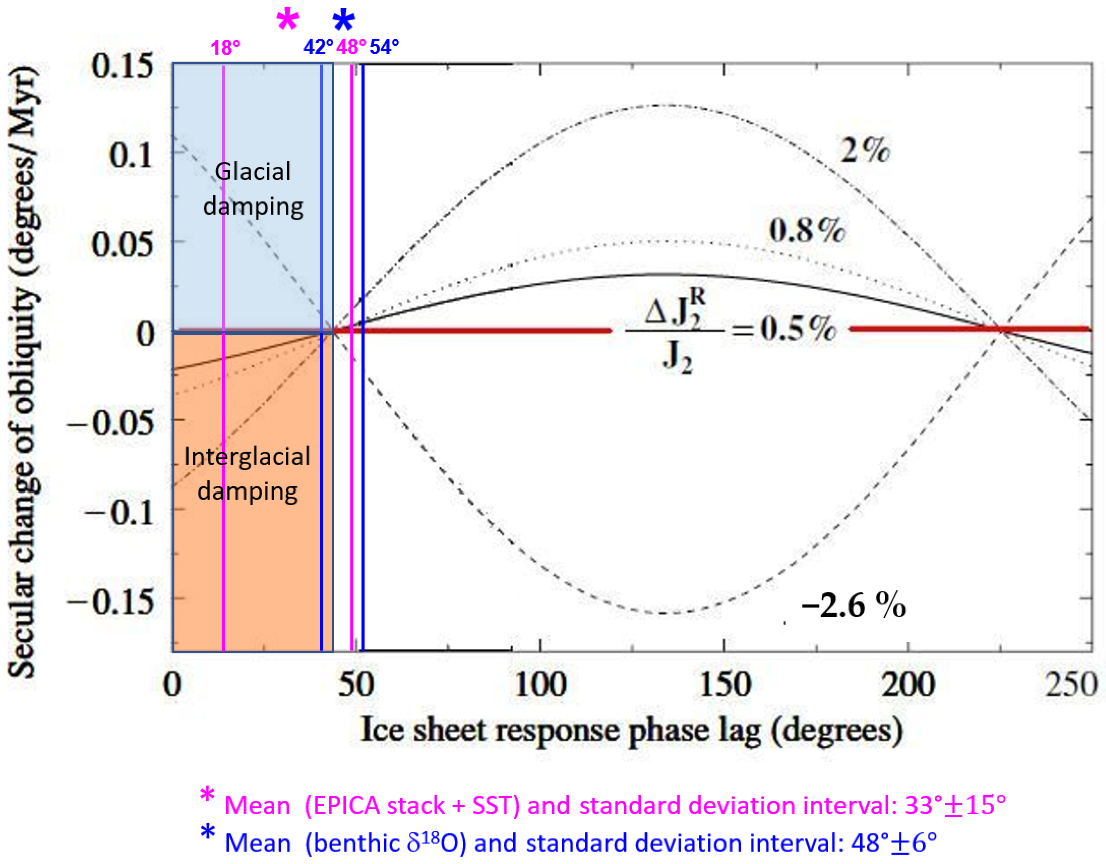
3.4.3. Changes in Earth’s Oblateness

Here, we have discussed how polar ice loading and global water mass redistribution might affect the changes in the Earth’s dynamic oblateness (J₂). Oblateness refers to the Earth’s ellipsoidal shape, i.e., its equatorial radius is ∼21 km larger than its polar radius, and most of this oblateness arises due to Earth’s rotation, which pushes its mass out towards the equator [121,122].

In particular, J₂ changes are determined by both glacial isostatic adjustment (GIA) and the gravitational redistribution of water in the oceans and atmosphere (W). GIA describes the response of the solid Earth, the gravitational field, and the oceans to mass changes in the global ice sheets [123]. A commonly studied component of GIA is ‘postglacial rebound’, which specifically relates to the uplifting of the land surface following ice melt, resulting in a decrease in J₂ [123,124,125,126,127,128]. A negative trend indicates that the Earth is becoming less oblate. During the deglaciation stage, water-ice masses are transferred from the polar regions to the global oceans, thereby increasing the polar moment of inertia and hence the J₂ [46,121]. Simulations conducted by Bills [43] suggest that the mass transport from the oceans to the polar ice sheets during Late Pleistocene glaciations can significantly change the gravitational oblateness of the Earth. The author concludes that it may be plausible that the MPT involves an obliquity–oblateness feedback, reflecting the evolution of the orbital–rotational–climatic system away from obliquity-dominated oscillations. The present-day variations in temporal gravity estimated by Earth satellite observations offer the opportunity to measure the ongoing changes in J₂. Nerem and Wahr [122] use present-day gravity variations from the gravity recovery and climate experiment (GRACE) satellite mission to investigate changes in a 34-year time series of the Earth’s oblateness observed by satellite laser ranging. The authors observed that, from 1975 to 1997, the oblateness variability exhibits a secular negative trend, which is believed to be due to postglacial rebound. It is worth noting that their results suggest that, since 2002, the ice loss from Greenland and Antarctica has remained the dominant contributor to the current GIA-corrected positive J₂ trend, which apparently began at some time during the 1990s. Similar results are reported by Seo et al. [127] over the period 1979–2010, which establishes that the variations in ice mass in Greenland and Antarctica have remained the dominant cause of the observed positive J₂ trend since 1998. Interestingly, the residual J₂ variations show a clear oscillation near 10–11 yr, suggesting some connection with solar activity [127] and thus a high sensitivity of the oblateness changes. Cheng et al. [126] reported an evident deceleration in the rate of the GIA-induced decrease in J₂ over the last few decades, and this is due to changes in the rate of the global mass redistribution from the melting of the glaciers and ice sheets, as well as mass changes in the atmosphere and ocean. Also, Nakada and Okuno [128] estimated the total positive J₂ change of Greenland–Antarctic ice sheets and mountain glaciers, and attested the change to recent melting models. It is worth noting that Sun et al. [129] and Sun and Riva [130] proposed an approach to simultaneously estimate J₂ temporal variations based on gravity observations from the GRACE satellite mission. One of the main advantages of their methodology is that it allows one to separate the quantitative contributions of individual sources to the total signal. They found that the secular trend is mainly generated by 1) ice-sheet melt (primarily controlled by Greenland, mountain glaciers, and Antarctica, respectively), which has a positive J₂ change, and 2) the ongoing solid Earth response to past glaciation (GIA component), which has a negative trend. In particular, the trend due to ice-sheet melting during 2002–2017 has a larger absolute value, such that the overall trend is rising and the Earth is currently becoming flatter. More specifically, by using the J₂ estimates from Table 2 of Sun and Riva [130], we calculated the contribution of the J₂ water layer to be ∼70% over the total absolute J₂ signal in 13 years only (2003–2016). A recent study on the last interglacial (MIS-5e) found that colder North Atlantic surface water and weaker Atlantic overturning characterised the early last interglacial (126 kyr) compared to the late last interglacial episode (122 kyr) [131]. Also, the δ¹⁸O values from the Greenland ice cores show a multimillennial lagged response to summer insolation during the early part of MIS-1 and MIS-5e interglacials, which may be explained by changes in ice-sheet elevation and the impact of meltwater on ocean circulation [132]. These results from past interglacial stages suggest that both insolation and ice-sheet melting have to be considered to reproduce the climatic pattern, and especially point out a relevant role of meltwater flux in interglacial dynamics. In particular, the remarkable result of the cross-spectral analysis of the ESL of the Red Sea (Figure 22, Table 5) suggests a rapid and coherent oscillation in the obliquity band of the water layer component of the Earth’s oblateness.

These studies are outstanding because they indicate a high sensitivity of the Earth to variations in oblateness that is induced by the fast response of the cryosphere mass balance to surface temperature changes. In addition, they highlight a concurrent slow moderate negative (GIA rebound) and fast robust positive (water mass redistribution) J₂ change in the recent postglacial and global warming context, resulting in a J₂ positive net change. The secular obliquity change depends only on the amplitude and phase lags of the oblateness variations in the obliquity band [46]. Thus, it can be speculatively affirmed that during the Plio–Pleistocene long-term cooling trend, it was the rapid and quantitatively dominant water mass redistribution component that controlled the J₂ net change in the obliquity band. This water mass redistribution component, which is reasonably related to the glacio-eustatic variations in the sea level, could be a crucial element in determining the J₂ positive net change during obliquity maxima. In this sense, the strong coherence between the Red Sea ESL and the global δ¹⁸O in the obliquity band (Table 5) is very significant. Also, the good congruence between the ESL and EPICA in terms of the rescaled variance during the last 500 kyr (Table 3) suggests similarities in amplitude patterns. It is therefore plausible to assume that the chaining ‘forcing > surface temperature > feedbacks > ice volume > ESL > J₂ water mass redistribution’ in the obliquity band during the Plio–Pleistocene was dominant over the solid Earth’s response with an amplitude pattern similar to that of the SST-δ¹⁸O, characterised by transient phases of progressive amplitude increases linked to the icy state (Figure 6 and Figure 18). Following the work of Sun and Riva [130] and assuming obliquity phase lag <5 kyr, we can schematically approximate the effect of the obliquity–oblateness feedback as follows:

High ε (interglacial): ΔJ₂ = −GIA₃₀ +W₇₀ ≈ +W ⟹ −Δε ⟹ interglacial damping,

Low ε (glacial): ΔJ₂ = +GIA₃₀ − W₇₀ ≈ −W ⟹ +Δε ⟹ glacial damping,

where ε refers to obliquity; ΔJ₂ is the net change in oblateness; GIA₃₀ reflects the slow moderate GIA component of oblateness; W₇₀ is the fast robust water component of oblateness; and Δε is the secular change in obliquity. It should be considered that a strong variation in the obliquity is probably not necessary owing to the exponential behaviour of climate responses caused by feedback mechanisms [7,8,12,24,26,31,40,66,88,93]. The pre-MPT amplification of the obliquity R_s (δ¹⁸O, SST) with the development of the icy state (Figure 6d, blue bars) might have led to the increase in the amplitude of both the glacio-eustatic oscillation and the oblateness change related to the dominant and fast water mass redistribution component. This possible step-wise increase in amplitude of the obliquity-paced J₂ net change within each transition interval (TRA-1, 2, 3), along with obliquity phase lags that may also be below the theoretical threshold of 44°, might have reached J₂-sensitive values. This might have induced secular changes in obliquity, each culminating in a ‘reversal’ of obliquity weakening that favoured the strengthening of the short eccentricity response by feedbacks amplification (Figure 6d, red bars). In an icy-state background, the most critical stage of this phenomenon is during obliquity maxima (interglacials) with the consequent weakening of the obliquity ice killing and strengthening of the ~100 kyr long-life feedbacks-induced ice growth. The maximum expression of this mechanism would occur during the TRA-3, which is associated with the maximum development of the icy state (subtrend IV) and strong amplification of the obliquity response up to the MPT end (TH4). TRA-1 and TRA-2 would be early precursor stages of this complex mechanism that was initiated as early as during the ONHG.

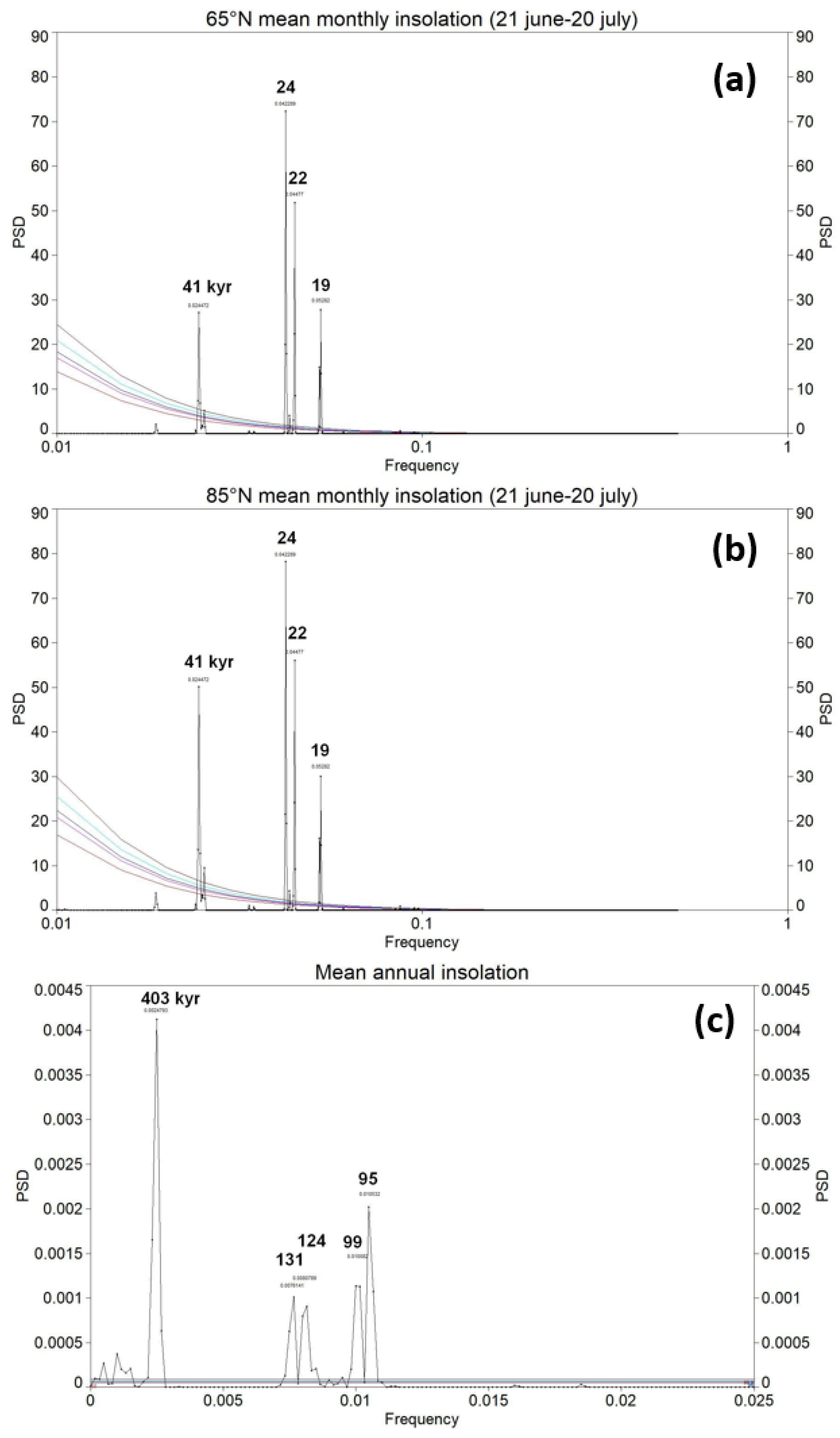
3.5. Earth’s Eccentricity and the 100,000-Year Issue

Milankovitch’s theory describes climate cycles controlled by high-latitude NH summer insolation, which results from the collective effects of changes in the Earth’s movements (eccentricity, obliquity, precession) over thousands of years. Although broadly accepted, some specific observations are not explained by the theory. For a discussion, see [10,59]. Here, we focus our discussion on the role of the short eccentricity, which is closely related to the MPT conundrum. Since the historical work of Hays et al. [72], the 100,000-year issue is derived by the observation that 65° N mean monthly insolation (21 June–20 July) is dominated by precession (24-22-19 kyr, 85% power) and secondarily by obliquity (41 kyr, 15% power), while eccentricity is negligible (Figure 23a). The frequency spectrum does not change significantly if we consider the 85° N mean monthly insolation, where we observe an increase in the obliquity power (23%) over precession (77%) (Figure 23b).

Indeed, the eccentricity primarily controls the amplitude of the precession cycle [10,133]. However, the eccentricity, through altering the mean distance from the Earth to the Sun, is the only orbital parameter that changes the Earth’s mean annual insolation (MAI), although the total energy received is very small quantitatively [10,37,133] (Figure 23c). But, unexpectedly compared to the theory, variance analysis of climate proxies such as EPICA shows the opposite picture with respect to the nominal forcings, with the short eccentricity dominating (51.6%), followed by obliquity (19%), and, lastly, precession (8.4%) [26]. Hence, the main paradox of the Milankovitch theory concerns (1) the marginal magnitude of precession in proxies compared to the dominant high-latitude NH summer insolation, (2) the origin of the short eccentricity glacial periodicity (which is negligible on high-latitude NH summer insolation), and (3) the strength of the short eccentricity component in climate proxies with respect to the forcing. Concerning the latter, Hays et al. [72] wrote “… an explanation of the correlation between climate and eccentricity probably requires an assumption of nonlinearity”. R_s analyses by Viaggi [8] and in the present work (Table 1 and Table 5), which suggest that the climate system is not self-sustaining because the variance in the response does not match the variance in the forcing, clearly corroborate this statement. Thus, orbitally paced climate responses likely result from nonlinear changes through the combined action of internal feedback mechanisms (albedo, GHGs, etc.) that are dependent on the mean climate state and are especially linked to the duration of orbital cycles (i.e., exponential coefficient e^kx of Viaggi [8]; see also Sect. 3.1.3 ‘R_s orbital factor model’), operating a strong energy transfer [7,9,24,26,31,72,86,89,91,93,94]. According to Ellis and Palmer [10], glacial cycles are forced by orbital cycles and Milankovitch insolation, but regulated by ice-albedo and dust-albedo feedbacks. A corollary of Milankovitch’s theory is that the climatic effect of orbital forcings must be in a phase and consequent to the cause because the climate system is inertial. As already argued by Hays et al. [72], “the dominant 100,000-year climatic component has an average period close to, and is in phase with, orbital eccentricity”, but this result has over time been marginalised mainly because of the low insolation fraction in the eccentricity band. Here, it is the case to highlight how the new cross-spectrum analysis data between nominal forcings and the respective components of global δ¹⁸O, Red Sea RSL (Table 5), and EPICA stacks (

Table 6. Data of cross-spectral analysis (Hann window) among nominal forcings (eccentricity La2010, [38]; obliquity, precession, and mean annual insolation La2004, [37]) and related EPICA stacks [26] for the last 800 kyr. Nominal precession inverted to align the climate polarity. Records rescaled in the range −1 to 1. Uniform sampling interval at 0.5 kyr. Negative phase values indicate that the signal lags forcing. Records are with their own time scale.

Forcing	EPICA Signal	Cross-Spectrum Freq. (kyr−1)	Cross-Spectrum Period (kyr)	Coherency	Phase Shift (Deg, kyr)
Eccentricity	Short ecc. stack	0.01125	88.9	0.94	17.4	4.30	EPICA signal leads
Short eccentricity 1	Short ecc. stack	0.01125	88.9	0.94	18.3	4.52	EPICA signal leads
Mean annual insolation (short eccentricity 1)	Short ecc. stack	0.01	100.0	0.72	13.8	3.83	EPICA signal leads
Obliquity	Obliquity stack	0.025	40.0	0.98	−37.9	−4.21	EPICA signal lags
Precession	Precession stack	0.0425	23.5	0.67	−60.8	−3.97	EPICA signal lags

¹ The 400 kyr band filtered out by wavelet analysis.

, Figure 24) confirm the high cospectral coherence of the 90–100 kyr cycle also, and a general delayed pattern of proxies consistent with an inertial climate system (with the only exception of the EPICA short eccentricity; see discussion below). In particular, it should also be noted that the weak short eccentricity component of the MAI has a coherence of 0.72 (Table 6), and that the La2010 nominal short eccentricity signal acquired from Morlet wavelet filtering has a high cross-coherency with the associated components of global benthic δ¹⁸O (0.75) and the Red Sea RSL (0.78) during the last 500 kyr (Table 5). Assuming a certain margin of error due to different age models, the phase delay of EPICA obliquity and precession stacks with respect to nominal forcings (4.2 kyr and ~4.0 kyr, respectively) is in agreement with the putative cause–effect relationship, and supports the action of feedback mechanisms, which are lagged by definition [8,26]. On the other hand, the EPICA short eccentricity stack shows an advance of 4.3–4.5 kyr, which seems noncredible. Instead, the phase relationships of the short eccentricity within the EPICA record (i.e., with the same age model) are consistent with an inertial climate system affected by feedbacks since CO₂ and CH₄ lags δD [26]. The EPICA ‘anomalous’ result with the eccentricity nominal solution could be an artefact owing to the averaging of the lead-lag phase variability over a small number of short eccentricity peaks (16) during the last 800 kyr, perhaps in relation to possible inaccuracies in the age model and error propagation on long periodicity.

Nevertheless, these short eccentricity cospectral data cannot be undervalued simply because the energy involved is too low. Presumably, there are other different and complex mechanisms at stake that we have probably underestimated, like feedback mechanisms. On the other hand, the weaker short eccentricity external forcing should not imply any problem if the ~100 kyr response is driven primarily by internal feedbacks that transfer most of the climate system energy [7,8,22,24,26,72,86,134]. In particular, Shackleton [24] believes that the ~100 kyr cycle is not generated from ice-sheet dynamics but that it is probably the effect of orbital forcing eccentricity, with the changing atmospheric CO₂ concentration influencing the global carbon cycle and controlling the timing of glaciations [23], and Lisiecki [7] points towards an internally driven climate response phase-locked to eccentricity.

It is the author’s strong belief that the reason for the paradox of Milankovitch’s theory lies in the difference between a forcing-centric and a response-centric paradigm, with feedback mechanisms in between. They make the difference since precession, although energetically relevant, is a short hemicycle in which feedbacks have less time to transfer additional energy (precession e^kx for the LR04 δ¹⁸O is 1.78 vs. 2.93 for the short eccentricity). Obliquity, although much weaker in the NH insolation spectrum, has a longer cycle that favours a more consistent feedbacks-mediated thermal response (e^kx = 1.88). So, it could be that an ice sheet that manages to survive the ablation of precession and obliquity could be sensitive to feedbacks mediated by short eccentricity.

In this context, the ODH comes into play as it offers a possible physical mechanism that mitigates the obliquity forcing, which is the main summer ice-melt agent at NH high latitudes as previously discussed. This mechanism, by favouring a longer life of the ice sheet through the obliquity-cycle damping and ‘skipping’, combined with the Earth’s long-term cooling, may have increased the sensitivity of the polar climate system to the minima of MAI by triggering a strong feedback-related nonlinear energy transfer in the short eccentricity band.

4. Summary and Conclusions

4.1. Main Results

The evidence of obliquity damping based on proxy records can be summarised as follows:

• The Antarctic orbital R_s demonstrates that, since 560 kyr, a strong amplification of the short eccentricity signals has been occurring (up to 400%, 600%) coupled with the damping of obliquity responses (up to −80%, −60%), confirming the marked asymmetry of the climate responses to orbital forcing. The PCA model of R_s data (EPICA, LR04 δ¹⁸O) suggests PC-1 to be a latent factor, indicating a post-MPT anticorrelation among obliquity and short eccentricity/precession R_s that is related to the long-term growth of the cryosphere volume.
• The PCA model integrating Plio–Pleistocene orbital R_s data and the long-term components of both LR04 δ¹⁸O and Site 846 SST records identify two PCs that are strictly related to the δ¹⁸O/SST short eccentricity/precession (PC-1) and obliquity (PC-2) amplification. Both are linked to the long-term δ¹⁸O enrichment and SST reduction. PC-2 factor highlights the post-MPT anomalous depletion of the obliquity R_s. These factors corroborate the latent link among the increasing amplitude of all orbital climate responses, the obliquity damping, and the Earth’s icy state developed through four stages of step-wise growth (subtrend I to IV).
• The spread of Plio–Pleistocene PCs exhibits two anticorrelation patterns of increasing absolute magnitude among forcing responses through time: a positive spread showing high obliquity associated with low short eccentricity/precession R_s, and a negative spread showing low obliquity linked to high short eccentricity/precession R_s. These response configurations are associated with three transition patterns of positive-to-negative spread including ONHG (Transition-1), INHG (Transition-2), and MBE (Transition-3), the latter being characterised by an extremely high magnitude and containing the MPT.
• EPICA orbital SSA stacks, which are rescaled on Plio–Pleistocene variance, exhibit a short eccentricity estimate of 12.2%, which is very high compared to the global δ¹⁸O value of 6.5%. In addition, an obliquity estimate of 4.5% is very low compared to the δ¹⁸O value of 9.9%. This is in agreement with the results of the R_s analysis, indicating a post-MPT short eccentricity amplification vs. obliquity damping.
• Orbital SSA components from the RSL record of the Red Sea exhibit a Plio–Pleistocene rescaled variance consistent with that of EPICA: short eccentricity (14.5%), obliquity (3.1%), and precession (2.8%). These data suggest post-MPT short eccentricity amplification vs. obliquity damping even in ESL fluctuations.
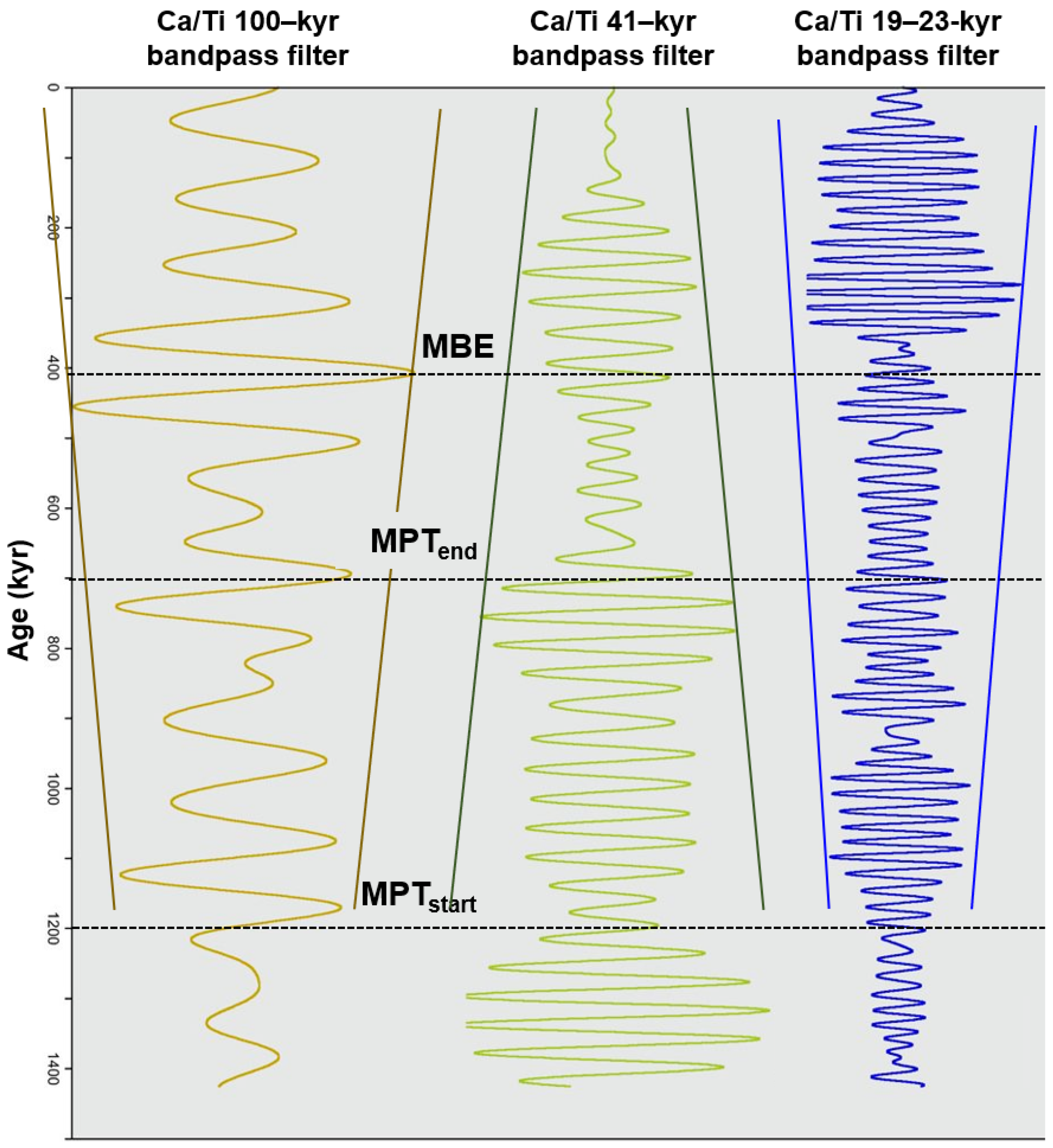
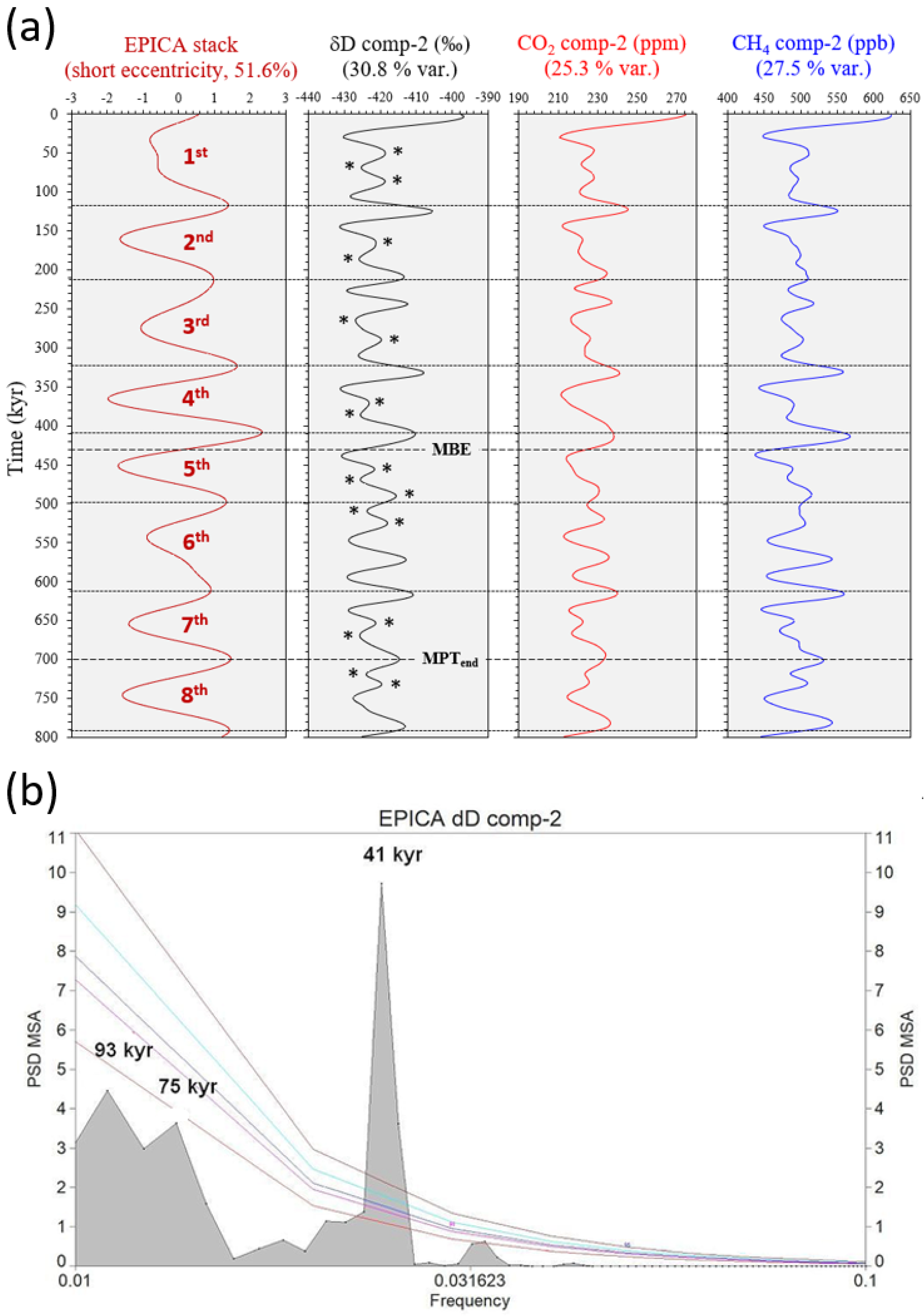
• Antarctic SSA structural signal observations of two or three low-amplitude 41 kyr obliquity peaks (glacial/interglacial) embedded in a weak ~93/75 kyr short eccentricity framework determined from δD, CO₂, and CH₄ component-2s are very similar in shape to the global LR04 δ¹⁸O and Site 846 equatorial Pacific SST component-3–4s during the MPT. These shapes may be further evidence of an obliquity attenuation phenomenon linked to the short eccentricity, and seem observationally reminiscent of the ‘obliquity-cycle skipping’ model.
• Additional evidence of MPT and post-MPT anticorrelation between obliquity damping and short eccentricity amplification is highlighted from a variety of global and regional (Atlantic, Pacific, Mediterranean, Indian) climate-related records, hinting that they are a widespread feature of the Pleistocene climate system. However, this feature does not seem to be consistent with the nominal solutions.

The main results and considerations concerning the theoretical constraints required by ODH can be summarised as follows:

• Studies on Greenland and Antarctica indicate a fast response of the cryosphere mass balance to recent atmospheric and SST changes. The EPICA stack_s better approximate the global benthic δ¹⁸O, where the latter probably represents the most lagged signal in the climate chain and may be considered a proxy of the global atmospheric temperature averaged by GHGs. Thus, the phase lags averaged among surface temperature proxies approximate the phase lag of the ice volume better, overcoming the deep temperature lag bias of the benthic δ¹⁸O.
• Assuming a fast response of the ice volume to surface temperature changes (EPICA stack, SST), the mean value of obliquity lag <5.0 kyr (3.7 ± 1.7 kyr) has been documented during the last 800 kyr. Also, considering the benthic δ¹⁸O records, the obliquity mean phase lag is 5.3 ± 0.6 kyr, which is very close to the theoretical threshold of 5.0 kyr and is significantly lower than the range of 6–10 kyr considered in previous studies.
• Cross-coherency data demonstrate that the Red Sea RSL record approximates extremely well the glacio-eustatic sea-level fluctuations linked to ice volume and paced by orbital forcings, also in the short eccentricity band. Global benthic δ¹⁸O lags Red Sea ESL by ~2.0 kyr in the obliquity band, suggesting a delay bias that could be attributed to the benthic δ¹⁸O deep-water temperature signal. Thus, the benthic δ¹⁸O obliquity mean phase lag of 5.3 kyr could be corrected to 3.3 kyr, close to the EPICA stack/SST mean of 3.7 kyr, which is significantly lower than the theoretical threshold of 5 kyr.
• Recent studies on variations in present-day satellite temporal gravity suggest the high sensitivity of the Earth to oblateness and highlight concurrent slow moderate negative (GIA rebound) and fast robust positive (water mass redistribution) J₂ changes during the recent postglacial and global warming context, resulting in a J₂ positive net change. Cross-spectral results from the Red Sea RSL over the last 500 kyr suggest a rapid and coherent oscillation in the obliquity band of the water layer component of the Earth’s oblateness.
• It is hypothesised that the fast and robust J₂ water mass redistribution component in the obliquity band, which is reasonably related to the glacio-eustatic variation in the sea level, could be a crucial element in determining +ΔJ₂ ⟹ −Δε during obliquity maxima (interglacial damping), and −ΔJ₂ ⟹ +Δε during obliquity minima (glacial damping). This explains the fact that obliquity damping in climate proxies is basically symmetrical.

4.2. Obliquity Damping Hypothesis

The proposed hypothesis can be outlined as follows:

• The widespread evidence from proxy records of anticorrelation between obliquity and short eccentricity/precession has been interpreted as an effect of the obliquity–oblateness feedback by critically reviewing its theoretical constraints, which support negative/positive secular change in obliquity for both low ice-volume phase lag (<5.0 kyr) and positive/negative net change in oblateness, respectively, in the obliquity band, that are likely dominated by the J₂ water mass redistribution component.
• Obliquity damping during the interglacial stages might have contributed to the strengthening of the short eccentricity response by mitigating the obliquity’s ice killing, favouring the obliquity-cycle skipping, and a ~100 kyr long-life feedback amplified ice growth in the context of the global icy state.
• Orbitals, including short eccentricity, may pace the frequency beat of the climate response. The phase-locked feedback mechanisms might have nonlinearly transferred most of the system energy depending on the long-term climate state and the cycle duration, overcoming the energy excess ‘paradox’, especially with respect to the eccentricity band.
• The observed transition patterns (TRA-1,-2,-3) of the orbitals R_s and the early onset of the short eccentricity response suggest the traditional notion of the MPT to be the final, high-magnitude, nonlinear transitional stage of a complex competing interaction between obliquity and short eccentricity forcing under the influence of both long-term cooling and obliquity–oblateness feedback that had already started during the Piacenzian. The maximum expression of this mechanism occurs during TRA-3, which is associated with the maximum ice-volume development (subtrend IV) and a strong amplification of the obliquity response until the termination of the MPT (TH4).
• The Plio–Pleistocene long-term cooling is a relevant background forcing in setting boundary conditions to orbital climate responses, and is characterised by four step-wise subtrends (I to IV), where a mild curvilinear shape is broken by slope changes representing four thresholds (TH1 to TH4) of mean climate state change.
• The role of the long-term cooling is outlined as follows:
  • The nonlinearity of the orbital responses is increased by the scale effect of the ice-sheet growth on feedback mechanisms, which are sensitive to long orbital periods. Specifically, the amplitude increases in the obliquity band of the ice-volume changes. It is hypothesised that the glacio-eustatic oscillations in the obliquity band inducing oblateness variations by the dominant/fast water mass redistribution component could have led to the overcoming of the thresholds sensitive to secular changes in obliquity. This mechanism would explain why the 100 kyr cycle reached its maximum expression post-MPT, albeit after a period of early/weak manifestations as early as in the Piacenzian.
  • The icy state may have increased the sensitivity of the polar climate system to the minima of MAI by triggering a strong nonlinear energy transfer in the short eccentricity band by feedback mechanisms (primarily albedo and GHGs).

The coupling between obliquity damping and short eccentricity amplification through the long-term cooling is a missing link in the Pleistocene climate system and MPT debate. The ODH could explain the rise of a dominant ~100 kyr response during the Mid-Late Pleistocene as its enhanced sensitivity to short eccentricity by a competing interaction with obliquity through an obliquity–oblateness feedback mechanism during the development of the Earth’s icy state. This suggests a different impact of the climate friction than previously thought.

4.3. Outlook

The ODH needs corroboration studies. Here, we make some recommendations for future research:

• Unbiased estimates of the ice-volume lag in the obliquity band.
• Modelling the changes in Earth’s oblateness in the obliquity band and its effects on the forcing, determined especially by considering the dominant/fast water mass redistribution component. This could make the difficult and uncertain solid Earth’s oblateness component less stringent among the theoretical constraints.
• Modelling the hypothesis with full observational evidence control.
• Determining the role of the MAI and feedback mechanisms in the context of the Earth’s long-term icy state.

References

1. Head, M.J.; Gibbard, P.L. Early–Middle Pleistocene transitions: An overview and recommendation for the defining boundary. Geol. Soc. Lond. Spec. Publ. 2005, 247, 1–18. [Google Scholar] [CrossRef]
2. Clark, P.U.; Archer, D.; Pollard, D.; Blum, J.D.; Rial, J.A.; Brovkin, V.; Mix, A.C.; Pisias, N.G.; Roy, M. The middle Pleistocene transition: Characteristics, mechanisms, and implications for long-term changes in atmospheric pCO2. Quat. Sci. Rev. 2006, 25, 3150–3184. [Google Scholar] [CrossRef]
3. Head, M.J.; Pillans, B.; Farquhar, S.A. The Early–Middle Pleistocene transition: Characterization and proposed guide for the defining boundary. Episodes 2008, 31, 255–259. [Google Scholar] [CrossRef]
4. Imbrie, J.; Berger, A.; Boyle, E.A.; Clemens, S.C.; Duffy, A.; Howard, W.R.; Kukla, G.; Kutzbach, J.; Martinson, D.G.; Mcintyre, A.; et al. On the structure and origin of major glaciation cycles 2. The 100,000-year cycle. Paleoceanography 1993, 8, 699–735. [Google Scholar] [CrossRef]
5. Berger, A.; Loutre, M.F.; Li, X.S. Modeling northern hemisphere ice volume over the last 3 Ma. Quat. Sci. Rev. 1999, 18, 1–11. [Google Scholar] [CrossRef]
6. Berger, A.; Loutre, M. Modeling the 100-kyr glacial–interglacial cycles. Glob. Planet. Change 2010, 72, 275–281. [Google Scholar] [CrossRef]
7. Lisiecki, L.E. Links between eccentricity forcing and the 100,000-year glacial cycle. Nat. Geosci. 2010, 3, 349–352. [Google Scholar] [CrossRef]
8. Viaggi, P. δ18O and SST signal decomposition and dynamic of the Pliocene-Pleistocene climate system: New insights on orbital nonlinear behavior vs. long-term trend. Prog. Earth Planet. Sci. 2018, 5, 81. [Google Scholar] [CrossRef]
9. Bintanja, R.; van de Wal, R.S.W. North American ice-sheet dynamics and the onset of 100,000-year glacial cycles. Nature 2008, 454, 869–872. [Google Scholar] [CrossRef]
10. Ellis, R.; Palmer, M. Modulation of ice ages via precession and dust-albedo feedbacks. Geosci. Front. 2016, 7, 891–909. [Google Scholar] [CrossRef]
11. Chalk, T.B.; Hain, M.P.; Foster, G.L.; Rohling, E.J.; Sexton, P.F.; Badger, M.P.S.; Cherry, S.G.; Hasenfratz, A.P.; Haug, G.H.; Jaccard, S.L.; et al. Causes of ice age intensification across the Mid-Pleistocene Transition. Proc. Natl. Acad. Sci. USA 2017, 114, 13114–13119. [Google Scholar] [CrossRef] [PubMed]
12. Köhler, P.; van de Wal, R.S.W. Interglacials of the Quaternary defined by northern hemispheric land ice distribution outside of Greenland. Nat. Commun. 2020, 11, 1–10. [Google Scholar] [CrossRef] [PubMed]
13. Imbrie, J.; Imbrie-Moore, A.; Lisiecki, L.E. A phase-space model for Pleistocene ice volume. Earth Planet Sci. Lett. 2011, 307, 94–102. [Google Scholar] [CrossRef]
14. Crucifix, M. Oscillators and relaxation phenomena in Pleistocene climate theory. Philos. Trans. R. Soc. A Math. Phys. Eng. Sci. 2012, 370, 1140–1165. [Google Scholar] [CrossRef] [PubMed]
15. Ditlevsen, P.D.; Ashwin, P. Complex Climate Response to Astronomical Forcing: The Middle-Pleistocene Transition in Glacial Cycles and Changes in Frequency Locking. Front. Phys. 2018, 6, 62. [Google Scholar] [CrossRef]
16. Quinn, C.; Sieber, J.; von der Heydt, A.S.; Lenton, T.M. The Mid-Pleistocene Transition induced by delayed feedback and bistability. Dyn. Stat. Clim. Syst. 2018, 3, dzy005. [Google Scholar] [CrossRef]
17. Mukhin, D.; Gavrilov, A.; Loskutov, E.; Kurths, J.; Feigin, A. Bayesian Data Analysis for Revealing Causes of the Middle Pleistocene Transition. Sci. Rep. 2019, 9, 7328. [Google Scholar] [CrossRef]
18. Nyman, K.H.M.; Ditlevsen, P.D. The middle Pleistocene transition by frequency locking and slow ramping of internal period. Clim. Dynam. 2019, 53, 3023–3038. [Google Scholar] [CrossRef]
19. Berends, C.J.; Köhler, P.; Lourens, L.J.; van de Wal, R.S.W. On the Cause of the Mid-Pleistocene Transition. Rev. Geophys. 2021, 59, e2020RG000727. [Google Scholar] [CrossRef]
20. Huybers, P. Combined obliquity and precession pacing of late Pleistocene deglaciations. Nature 2011, 480, 229–232. [Google Scholar] [CrossRef]
21. Huybers, P. Glacial variability over the last two million years: An extended depth-derived agemodel, continuous obliquity pacing, and the Pleistocene progression. Quat. Sci. Rev. 2007, 26, 37–55. [Google Scholar] [CrossRef]
22. Liu, Z.; Cleaveland, L.C.; Herbert, T.D. Early onset and origin of 100-kyr cycles in Pleistocene tropical SST records. Earth Planet. Sci. Lett. 2008, 265, 703–715. [Google Scholar] [CrossRef]
23. Raymo, M.E. The timing of major climate terminations. Paleoceanography 1997, 12, 577–585. [Google Scholar] [CrossRef]
24. Shackleton, N.J. The 100,000-Year Ice-Age Cycle Identified and Found to Lag Temperature, Carbon Dioxide, and Orbital Eccentricity. Science 2000, 289, 1897–1902. [Google Scholar] [CrossRef] [PubMed]
25. Lisiecki, L.E.; Raymo, M.E. Plio–Pleistocene climate evolution: Trends and transitions in glacial cycle dynamics. Quat. Sci. Rev. 2007, 26, 56–69. [Google Scholar] [CrossRef]
26. Viaggi, P. Quantitative impact of astronomical and sun-related cycles on the Pleistocene climate system from Antarctica records. Quat. Sci. Adv. 2021, 4, 100037. [Google Scholar] [CrossRef]
27. Abe-Ouchi, A.; Saito, F.; Kawamura, K.; Raymo, M.E.; Okuno, J.; Takahashi, K.; Blatter, H. Insolation-driven 100,000-year glacial cycles and hysteresis of ice-sheet volume. Nature 2013, 500, 190–193. [Google Scholar] [CrossRef]
28. Zachos, J.C.; Pagani, M.; Sloan, L.; Thomas, E.; Billups, K. Trends, rhythms, and aberrations in global climate 65 Myr to present. Science 2001, 292, 686–693. [Google Scholar] [CrossRef]
29. Zachos, J.C.; Dickens, G.R.; Zeebe, R.E. An early Cenozoic perspective on greenhouse warming and carbon-cycle dynamics. Nature 2008, 451, 279–283. [Google Scholar] [CrossRef]
30. Kender, S.; Ravelo, A.C.; Worne, S.; Swann, G.E.A.; Leng, M.J.; Asahi, H.; Becker, J.; Detlef, H.; Aiello, I.W.; Andreasen, D.; et al. Closure of the Bering Strait caused Mid-Pleistocene Transition cooling. Nat. Commun. 2018, 9, 5386. [Google Scholar] [CrossRef]
31. Shoenfelt, E.M.; Winckler, G.; Lamy, F.; Anderson, R.F.; Bostick, B.C. Highly bioavailable dust-borne iron delivered to the Southern Ocean during glacial periods. Proc. Natl. Acad. Sci. USA 2018, 115, 11180–11185. [Google Scholar] [CrossRef]
32. Farmer, J.R.; Hönisch, B.; Haynes, L.L.; Kroon, D.; Jung, S.; Ford, H.L.; Raymo, M.E.; Jaume-Seguí, M.; Bell, D.B.; Goldstein, S.L.; et al. Deep Atlantic Ocean carbon storage and the rise of 100,000-year glacial cycles. Nat. Geosci. 2019, 12, 355–360. [Google Scholar] [CrossRef]
33. Hasenfratz, A.P.; Jaccard, S.L.; Martínez-García, A.; Sigman, D.M.; Hodell, D.A.; Vance, D.; Bernasconi, S.M.; Kleiven, H.F.; Haumann, F.A.; Haug, G.H. The residence time of Southern Ocean surface waters and the 100,000-year ice age cycle. Science 2019, 363, 1080–1084. [Google Scholar] [CrossRef]
34. Jicha, B.R.; Scholl, D.W.; Rea, D.K. Circum-Pacific arc flare-ups and global cooling near the Eocene-Oligocene boundary. Geology 2009, 37, 303–306. [Google Scholar] [CrossRef]
35. Steinberger, B.; Spakman, W.; Japsen, P.; Torsvik, T.H. The key role of global solid-Earth processes in preconditioning Greenland’s glaciation since the Pliocene. Terra Nova 2015, 27, 1–8. [Google Scholar] [CrossRef]
36. Daradich, A.; Huybers, P.; Mitrovica, J.; Chan, N.-H.; Austermann, J. The influence of true polar wander on glacial inception in North America. Earth Planet. Sci. Lett. 2017, 461, 96–104. [Google Scholar] [CrossRef]
37. Laskar, J.; Robutel, P.; Joutel, F.; Gastineau, M.; Correia, A.C.M.; Levrard, B. A long term numerical solution for the insolation quantities of the Earth. Astron. Astrophys. 2004, 428, 261–285. [Google Scholar] [CrossRef]
38. Laskar, J.; Fienga, A.; Gastineau, M.; Manche, H. La2010: A new orbital solution for the long-term motion of the Earth. Astron. Astrophys. 2011, 532, A89. [Google Scholar] [CrossRef]
39. Lisiecki, L.E.; Raymo, M.E. A Pliocene-Pleistocene stack of 57 globally distributed benthic δ18O records. Paleoceanography 2005, 20, PA1003. [Google Scholar] [CrossRef]
40. Herbert, T.D.; Peterson, L.C.; Lawrence, K.T.; Liu, Z. Tropical Ocean Temperatures Over the Past 3.5 Million Years. Science 2010, 328, 1530–1534. [Google Scholar] [CrossRef]
41. Rubincam, D.P. The obliquity of Mars and climate friction. J. Geophys. Res. 1993, 98, 10827–10832. [Google Scholar] [CrossRef]
42. Rubincam, D.P. Has climate changed the Earth’s tilt? Paleoceanography 1995, 10, 365–372. [Google Scholar] [CrossRef]
43. Bills, B.G. Obliquity-oblateness feedback: Are climatically sensitive values of obliquity dynamically unstable? Geophys. Res. Lett. 1994, 21, 177–180. [Google Scholar] [CrossRef]
44. Bills, B.G. An oblique view of climate. Nature 1998, 396, 405–406. [Google Scholar] [CrossRef]
45. Williams, D.M.; Kasting, J.F.; Frakes, L.A. Low-latitude glaciations and rapid changes in the Earth’s obliquity explained by obliquity–oblateness feedback. Nature 1998, 396, 453–455. [Google Scholar] [CrossRef] [PubMed]
46. Levrard, B.; Laskar, J. Climate friction and the Earth’s obliquity. Geophys. J. Int. 2003, 154, 970–990. [Google Scholar] [CrossRef]
47. Skinner, L.; Shackleton, N. An Atlantic lead over Pacific deep-water change across Termination I: Implications for the application of the marine isotope stage stratigraphy. Quat. Sci. Rev. 2005, 24, 571–580. [Google Scholar] [CrossRef]
48. Lisiecki, L.E.; Raymo, M.E. Diachronous benthic δ18O responses during late Pleistocene terminations. Paleoceanography 2009, 24, PA3210. [Google Scholar] [CrossRef]
49. Lisiecki, L.E. Atlantic overturning responses to obliquity and precession over the last 3 Myr. Paleoceanography 2014, 29, 71–86. [Google Scholar] [CrossRef]
50. Huybers, P. Early Pleistocene Glacial Cycles and the Integrated Summer Insolation Forcing. Science 2006, 313, 508–511. [Google Scholar] [CrossRef]
51. Raymo, M.E.; Nisancioglu, K.H. The 41 kyr world: Milankovitch’s other unsolved mystery. Paleoceanography 2003, 18, 1–15. [Google Scholar] [CrossRef]
52. Bajo, P.; Drysdale, R.N.; Woodhead, J.D.; Hellstrom, J.C.; Hodell, D.; Ferretti, P.; Voelker, A.H.L.; Zanchetta, G.; Rodrigues, T.; Wolff, E.; et al. Persistent influence of obliquity on ice age terminations since the Middle Pleistocene transition. Science 2020, 367, 1235–1239. [Google Scholar] [CrossRef]
53. Elderfield, H.; Ferretti, P.; Greaves, M.; Crowhurst, S.; McCave, I.N.; Hodell, D.; Piotrowski, A.M. Evolution of Ocean Temperature and Ice Volume Through the Mid-Pleistocene Climate Transition. Science 2012, 337, 704–709. [Google Scholar] [CrossRef] [PubMed]
54. Laskar, J.; Joutel, F.; Boudin, F. Orbital, precessional and insolation quantities for the Earth from −20 Myr to +10 Myr. Astron. Astrophys. 1993, 270, 522–533. [Google Scholar]
55. Jouzel, J.; Masson-Delmotte, V.; Cattani, O.; Dreyfus, G.; Falourd, S.; Hoffmann, G.; Minster, B.; Nouet, J.; Barnola, J.M.; Chappellaz, J.; et al. Orbital and Millennial Antarctic Climate Variability over the Past 800,000 Years. Science 2007, 317, 793–796. [Google Scholar] [CrossRef] [PubMed]
56. Lüthi, D.; Le Floch, M.; Bereiter, B.; Blunier, T.; Barnola, J.-M.; Siegenthaler, U.; Raynaud, D.; Jouzel, J.; Fischer, H.; Kawamura, K.; et al. High-resolution carbon dioxide concentration record 650,000–800,000 years before present. Nature 2008, 453, 379–382. [Google Scholar] [CrossRef]
57. Loulergue, L.; Schilt, A.; Spahni, R.; Masson-Delmotte, V.; Blunier, T.; Lemieux, B.; Barnola, J.-M.; Raynaud, D.; Stocker, T.F.; Chappellaz, J. Orbital and millennial-scale features of atmospheric CH4 over the past 800,000 years. Nature 2008, 453, 383–386. [Google Scholar] [CrossRef]
58. Bereiter, B.; Eggleston, S.; Schmitt, J.; Nehrbass-Ahles, C.; Stocker, T.F.; Fischer, H.; Kipfstuhl, S.; Chappellaz, J. Revision of the EPICA Dome C CO2 record from 800 to 600 kyr before present. Geophys. Res. Lett. 2015, 42, 542–549. [Google Scholar] [CrossRef]
59. Past Interglacials Working Group of PAGES. Interglacials of the last 800,000 years. Rev. Geophys. 2016, 54, 162–219. [Google Scholar] [CrossRef]
60. Bazin, L.; Landais, A.; Lemieux-Dudon, B.; Kele, H.T.M.; Veres, D.; Parrenin, F.; Martinerie, P.; Ritz, C.; Capron, E.; Lipenkov, V.; et al. An optimized multi-proxy, multi-site Antarctic ice and gas orbital chronology (AICC2012): 120–800 ka. Clim. Past 2013, 9, 1715–1731. [Google Scholar] [CrossRef]
61. Jouzel, J.; Alley, R.B.; Cuffey, K.M.; Dansgaard, W.; Grootes, P.; Hoffmann, G.; Johnsen, S.J.; Koster, R.D.; Peel, D.; Shuman, C.A.; et al. Validity of the temperature reconstruction from water isotopes in ice cores. J. Geophys. Res. 1997, 102, 26471–26487. [Google Scholar] [CrossRef]
62. Hodell, D.A.; Channell, J.E.T.; Curtis, J.H.; Romero, O.E.; Röhl, U. Onset of “Hudson Strait” Heinrich events in the eastern North Atlantic at the end of the middle Pleistocene transition (∼640 ka)? Paleoceanography 2008, 23, PA4218. [Google Scholar] [CrossRef]
63. Hodell, D.; Lourens, L.; Crowhurst, S.; Konijnendijk, T.; Tjallingii, R.; Jiménez-Espejo, F.; Skinner, L.; Tzedakis, P.; Abrantes, F.; Acton, G.D.; et al. A reference time scale for Site U1385 (Shackleton Site) on the SW Iberian Margin. Glob. Planet. Chang. 2015, 133, 49–64. [Google Scholar] [CrossRef]
64. Lawrence, K.T.; Herbert, T.D.; Brown, C.M.; Raymo, M.E.; Haywood, A.M. High-amplitude variations in North Atlantic sea surface temperature during the early Pliocene warm period. Paleoceanography 2009, 24, PA2218. [Google Scholar] [CrossRef]
65. Lawrence, K.; Sosdian, S.; White, H.; Rosenthal, Y. North Atlantic climate evolution through the Plio-Pleistocene climate transitions. Earth Planet. Sci. Lett. 2010, 300, 329–342. [Google Scholar] [CrossRef]
66. Russon, T.; Elliot, M.; Sadekov, A.; Cabioch, G.; Corrège, T.; De Deckker, P. The mid-Pleistocene transition in the subtropical southwest Pacific. Paleoceanography 2011, 26, A1211. [Google Scholar] [CrossRef]
67. Cheng, X.; Tian, J.; Wang, P. Data report: Stable isotopes from Site 1143. In Proceedings of the Ocean Drilling Program, Scientific Results; Prell, W.L., Wang, P., Blum, P., Rea, D.K., Clemens, S.C., Eds.; Ocean Drilling Program: College Station, TX, USA, 2004; Volume 184, pp. 1–8. [Google Scholar] [CrossRef]
68. Ao, H.; Dekkers, M.J.; Qin, L.; Xiao, G. An updated astronomical timescale for the Plio-Pleistocene deposits from South China Sea and new insights into Asian monsoon evolution. Quat. Sci. Rev. 2011, 30, 1560–1575. [Google Scholar] [CrossRef]
69. Li, L.; Li, Q.; Tian, J.; Wang, P.; Wang, H.; Liu, Z. A 4-Ma record of thermal evolution in the tropical western Pacific and its implications on climate change. Earth Planet. Sci. Lett. 2011, 309, 10–20. [Google Scholar] [CrossRef]
70. Konijnendijk, T.; Ziegler, M.; Lourens, L. On the timing and forcing mechanisms of late Pleistocene glacial terminations: Insights from a new high-resolution benthic stable oxygen isotope record of the eastern Mediterranean. Quat. Sci. Rev. 2015, 129, 308–320. [Google Scholar] [CrossRef]
71. Grant, K.M.; Rohling, E.J.; Ramsey, C.B.; Cheng, H.; Edwards, R.L.; Florindo, F.; Heslop, D.; Marra, F.; Roberts, A.P.; Tamisiea, M.E.; et al. Sea-level variability over five glacial cycles. Nat. Commun. 2014, 5, 5076. [Google Scholar] [CrossRef]
72. Hays, J.D.; Imbrie, J.; Shackleton, N.J. Variations in the Earth’s Orbit: Pacemaker of the Ice Ages. Science 1976, 194, 1121–1132. Available online: http://www.jstor.org/stable/1743620 (accessed on 5 January 2009). [CrossRef] [PubMed]
73. Steinhilber, F.; Abreu, J.A.; Beer, J.; Brunner, I.; Christl, M.; Fischer, H.; Heikkilä, U.; Kubik, P.W.; Mann, M.; McCracken, K.G.; et al. 9400 years of cosmic radiation and solar activity from ice cores and tree rings. Proc. Natl. Acad. Sci. USA 2012, 109, 5967–5971. [Google Scholar] [CrossRef] [PubMed]
74. Zharkova, V.V.; Shepherd, S.J.; Zharkov, S.I. Principal component analysis of background and sunspot magnetic field variations during solar cycles 21–23. Mon. Not. R Astron. Soc. 2012, 424, 2943–2953. [Google Scholar] [CrossRef]
75. Viaggi, P.; Scotti, P.; Previde Massara, E.; Knezaurek, G.; Menichetti, E.; Piva, A.; Torricelli, S.; Gambacorta, G. Paleoceanographic Evolution of mid-Cretaceous Paleobioproductivity and Paleoredox Chemometric Signals. Link to Cretaceous Long-term Eustatic Climax from a Central Atlantic Well Sequence. In Proceedings of the 3rd International Congress on Stratigraphy, Conference Presentation, STRATI 2019, Milan, Italy, 2–5 July 2019. [Google Scholar] [CrossRef]
76. Vautard, R.; Ghil, M. Singular spectrum analysis in nonlinear dynamics, with applications to paleoclimatic time series. Phys. D 1989, 35, 395–424. [Google Scholar] [CrossRef]
77. Elsner, J.B.; Tsonis, A.A. Singular Spectrum Analysis: A New Tool in Time Series Analysis; Springer: Berlin/Heidelberg, Germany, 1996. [Google Scholar]
78. Ghil, M.; Allen, R.M.; Dettinger, M.D.; Ide, K.; Kondrashov, D.; Mann, M.E.; Robertson, A.; Saunders, A.; Tian, Y.; Varadi, F.; et al. Advanced spectral methods for climatic time series. Rev. Geophys. 2002, 40, 3-1–3-41. [Google Scholar] [CrossRef]
79. Hassani, H. Singular spectrum analysis: Methodology and comparison. J. Data Sci. 2007, 5, 239–257. [Google Scholar] [CrossRef]
80. Lang, N.; Wolff, E.W. Interglacial and glacial variability from the last 800 ka in marine, ice and terrestrial archives. Clim. Past 2011, 7, 361–380. [Google Scholar] [CrossRef]
81. Barth, A.M.; Clark, P.U.; Bill, N.S.; He, F.; Pisias, N.G. Climate evolution across the Mid-Brunhes Transition. Clim. Past 2018, 14, 2071–2087. [Google Scholar] [CrossRef]
82. Berger, A.; Yin, Q. Modeling the interglacials of the last 1 million years. In Climate Change: Inferences from Paleoclimate and Regional Aspects; Berger, A., Mesinger, F., Sijacki, D., Eds.; Springer: Vienna, Austria, 2012. [Google Scholar]
83. Meyers, S.R.; Hinnov, L.A. Northern Hemisphere glaciation and the evolution of Plio-Pleistocene climate noise. Paleoceanography 2010, 25, A3207. [Google Scholar] [CrossRef]
84. McClymont, E.L.; Sosdian, S.M.; Rosell-Melé, A.; Rosenthal, Y. Pleistocene sea-surface temperature evolution: Early cooling, delayed glacial intensification, and implications for the mid-Pleistocene climate transition. Earth-Sci. Rev. 2013, 123, 173–193. [Google Scholar] [CrossRef]
85. Feng, F.; Bailer-Jones, C. Obliquity and precession as pacemakers of Pleistocene deglaciations. Quat. Sci. Rev. 2015, 122, 166–179. [Google Scholar] [CrossRef]
86. Viaggi, P. Evidence of Climate Mitigation Feedbacks by Global Forest Cover Expansion during the Pliocene. Int. J. Environ. Sci. Nat. Resour. 2021, 28, 556249. [Google Scholar] [CrossRef]
87. Berger, A.; Loutre, M.F. Long-term variations in insolation and their effects on climate, the LLN experiments. Surv. Geophys. 1997, 18, 147–161. [Google Scholar] [CrossRef]
88. Ruddiman, W.F. Orbital insolation, ice volume, and greenhouse gases. Quat. Sci. Rev. 2003, 22, 1597–1629. [Google Scholar] [CrossRef]
89. Archer, D.; Martin, P.; Buffett, B.; Brovkin, V.; Rahmstorf, S.; Ganopolski, A. The importance of ocean temperature to global biogeochemistry. Earth Planet. Sci. Lett. 2004, 222, 333–348. [Google Scholar] [CrossRef]
90. Rial, J.A.; Pielke, R.A., Sr.; Beniston, M.; Claussen, M.; Canadell, J.; Cox, P.; Held, H.; de Noblet-Ducoudré, N.; Prinn, R.; Reynolds, J.F.; et al. Nonlinearities, feedbacks and critical thresholds within the Earth’s climate system. Clim. Change 2004, 65, 11–38. [Google Scholar] [CrossRef]
91. Brovkin, V.; Ganopolski, A.; Archer, D.; Rahmstorf, S. Lowering of glacial atmospheric CO2 in response to changes in oceanic circulation and marine biogeochemistry. Paleoceanography 2007, 22, PA4202. [Google Scholar] [CrossRef]
92. Hansen, J.; Sato, M.; Kharecha, P.; Russell, G.; Lea, D.W.; Siddall, M. Climate change and trace gases. Philos. Trans. R. Soc. A Math. Phys. Eng. Sci. 2007, 365, 1925–1954. [Google Scholar] [CrossRef]
93. Köhler, P.; Bintanja, R.; Fischer, H.; Joos, F.; Knutti, R.; Lohmann, G.; Masson-Delmotte, V. What caused Earth’s temperature variations during the last 800,000 years? Data-based evidence on radiative forcing and constraints on climate sensitivity. Quat. Sci. Rev. 2010, 29, 129–145. [Google Scholar] [CrossRef]
94. Hansen, J.; Sato, M.; Kharecha, P.; von Schuckmann, K. Earth’s energy imbalance and implications. Atmos. Meas. Tech. 2011, 11, 13421–13449. [Google Scholar] [CrossRef]
95. Miller, G.H.; Alley, R.B.; Brigham-Grette, J.; Fitzpatrick, J.J.; Polyak, L.; Serreze, M.C.; White, J.W. Arctic amplification: Can the past constrain the future? Quat. Sci. Rev. 2010, 29, 1779–1790. [Google Scholar] [CrossRef]
96. Box, J.E.; Hubbard, A.; Bahr, D.B.; Colgan, W.T.; Fettweis, X.; Mankoff, K.D.; Wehrlé, A.; Noël, B.; Broeke, M.R.v.D.; Wouters, B.; et al. Greenland ice sheet climate disequilibrium and committed sea-level rise. Nat. Clim. Chang. 2022, 12, 808–813. [Google Scholar] [CrossRef]
97. Wunsch, C. Quantitative estimate of the Milankovitch-forced contribution to observed Quaternary climate change. Quat. Sci. Rev. 2004, 23, 1001–1012. [Google Scholar] [CrossRef]
98. Berger, A.; Mélice, J.L.; Loutre, M.F. On the origin of the 100-kyr cycles in the astronomical forcing. Paleoceanography 2005, 20, PA4019. [Google Scholar] [CrossRef]
99. Berger, A.; Yin, Q.Z.; Herold, N. MIS-11 and MIS-19, analogs of our Holocene interglacial. In Proceedings of the 3rd International Conference on Earth System Modelling, Hamburg, Germany, 17–21 September 2012; Available online: https://meetingorganizer.copernicus.org/3ICESM/3ICESM-11.pdf (accessed on 1 January 2016).
100. Martínez-Botí, M.A.; Foster, G.L.; Chalk, T.B.; Rohling, E.J.; Sexton, P.F.; Lunt, D.J.; Pancost, R.D.; Badger, M.P.S.; Schmidt, D.N. Plio-Pleistocene climate sensitivity evaluated using high-resolution CO2 records. Nature 2015, 518, 49–54. [Google Scholar] [CrossRef]
101. Hönisch, B.; Hemming, N.G.; Archer, D.; Siddall, M.; McManus, J.F. Atmospheric Carbon Dioxide Concentration Across the Mid-Pleistocene Transition. Science 2009, 324, 1551–1554. [Google Scholar] [CrossRef]
102. Seki, O.; Foster, G.L.; Schmidt, D.N.; Mackensen, A.; Kawamura, K.; Pancost, R.D. Alkenone and boron-based Pliocene pCO2 records. Earth Planet. Sci. Lett. 2010, 292, 201–211. [Google Scholar] [CrossRef]
103. Bartoli, G.; Hönisch, B.; Zeebe, R.E. Atmospheric CO2 decline during the Pliocene intensification of Northern Hemisphere glaciations. Paleoceanography 2011, 26, PA4213. [Google Scholar] [CrossRef]
104. Huybers, P.; Tziperman, E. Integrated summer insolation forcing and 40,000-year glacial cycles: The perspective from an ice-sheet/energy-balance model. Paleoceanography 2008, 23, PA1208. [Google Scholar] [CrossRef]
105. Yehudai, M.; Kim, J.; Pena, L.D.; Jaume-Seguí, M.; Knudson, K.P.; Bolge, L.; Malinverno, A.; Bickert, T.; Goldstein, S.L. Evidence for a Northern Hemispheric trigger of the 100,000-y glacial cyclicity. Proc. Natl. Acad. Sci. USA 2021, 118, e2020260118. [Google Scholar] [CrossRef]
106. Waelbroeck, C.; Levi, C.; Duplessy, J.-C.; Labeyrie, L.; Michel, E.; Cortijo, E.; Bassinot, F.; Guichard, F. Distant origin of circulation changes in the Indian Ocean during the last deglaciation. Earth Planet. Sci. Lett. 2006, 243, 244–251. [Google Scholar] [CrossRef]
107. Yin, Q.Z.; Berger, A. Individual contribution of insolation and CO2 to the interglacial climates of the past 800,000 years. Clim. Dyn. 2011, 38, 709–724. [Google Scholar] [CrossRef]
108. Masson-Delmotte, V.; Kageyama, M.; Braconnot, P.; Charbit, S.; Krinner, G.; Ritz, C.; Guilyardi, E.; Jouzel, J.; Abe-Ouchi, A.; Crucifix, M.; et al. Past and future polar amplification of climate change: Climate model intercomparisons and ice-core constraints. Clim. Dyn. 2005, 26, 513–529. [Google Scholar] [CrossRef]
109. Cuffey, K.M.; Clow, G.D. Temperature, accumulation, and ice sheet elevation in central Greenland through the last deglacial transition. J. Geophys. Res. 1997, 102, 26383–26396. [Google Scholar] [CrossRef]
110. Lemke, P.; Ren, J.; Alley, R.B.; Allison, I.; Carrasco, J.; Flato, G.; Fujii, Y.; Kaser, G.; Mote, P.; Thomas, R.H.; et al. Observations: Changes in Snow, Ice and Frozen Ground. In Climate Change 2007: The Physical Science Basis. Contribution of Working Group I to the Fourth Assessment Report of the Intergovernmental Panel on Climate Change; Solomon, S., Qin, D., Manning, M., Chen, Z., Marquis, M., Averyt, K.B., Tignor, M., Miller, H.L., Eds.; Cambridge University Press: Cambridge, UK; New York, NY, USA, 2007. [Google Scholar]
111. Hanna, E.; Huybrechts, P.; Steffen, K.; Cappelen, J.; Huff, R.; Shuman, C.; Irvine-Fynn, T.; Wise, S.; Griffiths, M. Increased Runoff from Melt from the Greenland Ice Sheet: A Response to Global Warming. J. Clim. 2008, 21, 331–341. [Google Scholar] [CrossRef]
112. Lawrence, D.M.; Slater, A.G.; Tomas, R.A.; Holland, M.M.; Deser, C. Accelerated Arctic land warming and permafrost degradation during rapid sea ice loss. Geophys. Res. Lett. 2008, 35, L11506. [Google Scholar] [CrossRef]
113. Ettema, J.; van den Broeke, M.R.; van Meijgaard, E.; van de Berg, W.J.; Bamber, J.L.; Box, J.E.; Bales, R.C. Higher surface mass balance of the Greenland ice sheet revealed by high-resolution climate modeling. Geophys. Res. Lett. 2009, 36, L12501. [Google Scholar] [CrossRef]
114. Tarnocai, C.; Canadell, J.G.; Schuur, E.A.G.; Kuhry, P.; Mazhitova, G.; Zimov, S. Soil organic carbon pools in the northern circumpolar permafrost region. Glob. Biogeochem. Cycles 2009, 23, GB2023. [Google Scholar] [CrossRef]
115. Yin, J.; Overpeck, J.T.; Griffies, S.M.; Hu, A.; Russell, J.L.; Stouffer, R.J. Different magnitudes of projected subsurface ocean warming around Greenland and Antarctica. Nat. Geosci. 2011, 4, 524–528. [Google Scholar] [CrossRef]
116. Pattyn, F.; Ritz, C.; Hanna, E.; Asay-Davis, X.; DeConto, R.; Durand, G.; Favier, L.; Fettweis, X.; Goelzer, H.; Golledge, N.R.; et al. The Greenland and Antarctic ice sheets under 1.5 °C global warming. Nat. Clim. Change 2018, 8, 1053–1061. [Google Scholar] [CrossRef]
117. King, M.D.; Howat, I.M.; Candela, S.G.; Noh, M.J.; Jeong, S.; Noël, B.P.Y.; van den Broeke, M.R.; Wouters, B.; Negrete, A. Dynamic ice loss from the Greenland Ice Sheet driven by sustained glacier retreat. Commun. Earth Environ. 2020, 1, 1. [Google Scholar] [CrossRef]
118. Tesi, T.; Asioli, A.; Previde Massara, E.; Montagna, P.; Pellegrini, C.; Nogarotto, A.; Cipriani, A.; Piva, A.; Muschitiello, F.; Rovere, M.; et al. Abrupt and persistent shutdown of the thermohaline forcing during MIS5e in the Adriatic Sea: Insights from shallow-water sapropel sediments. Quat. Sci. Adv. 2023, 13, 100134. [Google Scholar] [CrossRef]
119. Hilgen, F.J.; Lourens, L.J.; Berger, A.; Loutre, M.F. Evaluation of the astronomically calibrated time scale for the Late Piocene and the earliest Pleistocene. Paleoceanography 1993, 8, 549–565. [Google Scholar] [CrossRef]
120. Shackleton, N.J. Oxygen isotope analysis and pleistocene temperature reassessed. Nature 1967, 215, 15–17. [Google Scholar] [CrossRef]
121. Chao, B.F. Earth’s oblateness and its temporal variations. Comptes. Rendus Geosci. 2006, 338, 1123–1129. [Google Scholar] [CrossRef]
122. Nerem, R.S.; Wahr, J. Recent changes in the Earth’s oblateness driven by Greenland and Antarctic ice mass loss. Geophys. Res. Lett. 2011, 38, L13501. [Google Scholar] [CrossRef]
123. Whitehouse, P.L. Glacial isostatic adjustment modelling: Historical perspectives, recent advances, and future directions. Earth Surf. Dyn. 2018, 6, 401–429. [Google Scholar] [CrossRef]
124. Mitrovica, J.X.; Peltier, W.R. Present-day secular variations in the zonal harmonics of the Earth’s geopotential. J. Geophys. Res. 1993, 98, 4509–4526. [Google Scholar] [CrossRef]
125. Cheng, M.; Tapley, B.D. Variations in the Earth’s oblateness during the past 28 years. J. Geophys. Res. 2004, 109, B09402. [Google Scholar] [CrossRef]
126. Cheng, M.; Tapley, B.D.; Ries, J.C. Deceleration in the Earth’s oblateness. J. Geophys. Res. Solid Earth 2013, 118, 740–747. [Google Scholar] [CrossRef]
127. Seo, K.-W.; Chen, J.; Wilson, C.R.; Lee, C.-K. Decadal and quadratic variations of Earth’s oblateness and polar ice mass balance from 1979 to 2010. Geophys. J. Int. 2015, 203, 475–481. [Google Scholar] [CrossRef]
128. Nakada, M.; Okuno, J. Secular variations in zonal harmonics of Earth’s geopotential and their implications for mantle viscosity and Antarctic melting history due to the last deglaciation. Geophys. J. Int. 2017, 209, 1660–1676. [Google Scholar] [CrossRef]
129. Sun, Y.; Riva, R.; Ditmar, P.; Rietbroek, R. Using GRACE to Explain Variations in the Earth’s Oblateness. Geophys. Res. Lett. 2019, 46, 158–168. [Google Scholar] [CrossRef]
130. Sun, Y.; Riva, R.E.M. A global semi-empirical glacial isostatic adjustment (GIA) model based on Gravity Recovery and Climate Experiment (GRACE) data. Earth Syst. Dyn. 2020, 11, 129–137. [Google Scholar] [CrossRef]
131. Govin, A.; Braconnot, P.; Capron, E.; Cortijo, E.; Duplessy, J.C.; Jansen, E.; Labeyrie, L.; Landais, A.; Marti, O.; Michel, E.; et al. Persistent influence of ice sheet melting on high northern latitude climate during the early Last Interglacial. Clim. Past 2012, 8, 483–507. [Google Scholar] [CrossRef]
132. Masson-Delmotte, V.; Braconnot, P.; Hoffmann, G.; Jouzel, J.; Kageyama, M.; Landais, A.; Lejeune, Q.; Risi, C.; Sime, L.; Sjolte, J.; et al. Sensitivity of interglacial Greenland temperature and δ18O: Ice core data, orbital and increased CO2 climate simulations. Clim. Past 2011, 7, 1041–1059. [Google Scholar] [CrossRef]
133. Berger, A.; Loutre, M.; Tricot, C. Insolation and Earth’s orbital periods. J. Geophys. Res. Atmos. 1993, 98, 10341–10362. [Google Scholar] [CrossRef]
134. Rial, J.A. Pacemaking the Ice Ages by frequency modulation of Earth’s orbital eccentricity. Science 1999, 285, 564–568. [Google Scholar] [CrossRef]
Figure 1. Analysis of the orbital response sensitivity during the last 800 kyr (fuchsia: short eccentricity; brown: obliquity; green: precession) according to temporal segments binned at 80 kyr from EPICA: (a) δD; (b) CH4; (c) CO2; and (d) LR04 δ18O records. The balance line (0%) indicates that the variance in the response matches the variance in forcing, indicating a self-sustained climate system that is paced only by orbital forcings. Values significantly larger than zero indicate a reinforcement of the response signal. Negative Rs indicates a response variance lower than the orbital forcing, suggesting a damping mechanism for the climate system. Note the impressive asymmetry of the climate responses with extremely robust amplitude magnifications and moderate damping. Scale of the y-axis up to −200% for graphical requirements. MBE = Mid-Brunhes Event; MPT = Mid-Pleistocene transition. SSA components data are acquired from EPICA [26], LR04 [8]. Nominal solutions are from Laskar et al. [37] and Laskar et al. [38].
Geosciences 13 00354 g001
Figure 2. Standardised PCA model of EPICA δD, CO2, CH4, and LR04 δ18O orbital Rs during the last 800 kyr, binned at 80 kyr: (a) PC-1 loadings; (b) PC-1 regression factor score (black line), and δ18O exponential trend mean (green line). The asterisk indicates the transition to MBE. MBE = Mid-Brunhes Event; MPT = Mid-Pleistocene transition.
Geosciences 13 00354 g002
Figure 3. Morlet wavelet power spectra of EPICA SSA stacks: (a) short eccentricity; (b) obliquity; (c) precession. MBE = Mid-Brunhes Event; MPT = Mid-Pleistocene transition. Data from Viaggi [26].
Geosciences 13 00354 g003
Figure 4. (a) EPICA dominant short eccentricity stack (51.6% variance) and related cycles defined on maxima (black horizontal lines) and numbered from 1st to 8th (left), compared with δD, CO2, CH4 SSA-component-2 time series (obliquity signal embedded in a weak short eccentricity). Asterisks on δD comp-2 (not shown on the other comp-2s) exhibit two or three low-amplitude 41 kyr obliquity peaks (glacial/interglacial) embedded in a weak ~93/75 kyr framework after the MPT, a possible observational reminiscent of the ‘obliquity-cycle skipping’ [21]; (b) FFS of the δD comp-2, very similar to the CO2 and CH4 signals (not shown), showing a dominant 41 kyr cycle embedded in a weak ~93/75 kyr framework. Coloured lines are first-order autoregressive AR(1) curves (50%, 90%, 95%, 99%, and 99.9% significance levels). MBE = Mid-Brunhes Event; MPT = Mid-Pleistocene transition. Data from Viaggi [26].
Geosciences 13 00354 g004
Figure 5. Response sensitivity analysis of Pliocene–Pleistocene orbital components (blue: short eccentricity, brown: obliquity, green: precession) of (a,b) global LR04 δ18O and (c,d) equatorial ODP Site 846 SST as a function of the long-term mean climate state (left x-axis: exponential trend; right x-axis: long-term trend). The data are calculated from arbitrary time segments binned at 532 kyr. The balance line (0%) indicates that the variance of response matches the variance in forcing, suggesting a self-sustained climate system, which is only paced by orbital cycles. Values much larger than zero would indicate a reinforcement of the signal response. Note the different magnitude of amplification between the global LR04 δ18O (up to ~440%) and the equatorial Site 846 SST (up to ~180%) records. Negative Rs shows a response variance lower than orbital forcing, suggesting a damping mechanism for the climate system. The fuchsia box highlights the strong inverse coupling between obliquity damping and short eccentricity/precession amplification during post-MPT time. Data from Viaggi [8].
Geosciences 13 00354 g005
Figure 6. Pliocene–Pleistocene standardised PCA model for LR04 δ18O/Site 846 SST orbitals Rs and the mean climate state by time binned at 532 kyr: (a) PC-1 loadings; (b) PC-2 loadings; (c) PCs regression factor score (57.7% and 36.9% variance, respectively); (d) PCs factor score spread (PC-2–PC-1). Positive spread (blue bar): high obliquity vs. low short eccentricity/precession Rs. Negative spread (red bar): low obliquity vs. high short eccentricity/precession Rs. ONHG (Onset of the Northern Hemisphere Glaciation), INHG (Intensification of Northern Hemisphere Glaciation), MPT (Mid-Pleistocene Transition) and MBE label time bins containing these events. Blue arrows: transition patterns (TRA-1, 2, 3) of positive to negative factor spread including ONHG (TRA-1), INHG (TRA-2), and MPT/MBE (TRA-3). Data from Viaggi [8].
Geosciences 13 00354 g006
Figure 7. (a) Time-series panel of LR04 δ18O SSA component-2 (transition obliquity to short eccentricity) and its subcomponents (short eccentricity, obliquity). X-axis is scale variable (expressed in ‰); (b) FFS of comp-2 for three time intervals highlighted by red labelled boxes (p1, p2, p3). Coloured lines (50%, 90%, 95%, 99%, and 99.9% significance levels) are first-order autoregressive AR(1) curves to check statistically significant peaks vs. red/white noise background. The frequency scale is logarithmic. Note the transition in periodicity from obliquity (41–53 kyr) to short eccentricity (71–92 kyr) with a gradual upwards strengthening of the short eccentricity power. The amplitude of the short eccentricity in comp-2 subcomp-1–4, 9–15 increases (blue lines), whereas the amplitude of the obliquity in comp-2 subcomp-5–8 decreases after the MPTstart. ONHG = Onset of the Northern Hemisphere Glaciation; INHG = Intensification of Northern Hemisphere Glaciation; MPT = Mid-Pleistocene Transition. Figure 7a is modified after Viaggi [8]. δ18O SSA component-2 from Viaggi [8].
Geosciences 13 00354 g007
Figure 8. (a) Time-series panel of the ODP Site 846 SST component-2 (transition obliquity to short eccentricity) and component-3–4 (obliquity). X-axis scale variable (°C); (b) FFS of the comp-2 for three time intervals highlighted by red labelled boxes (p1, p2, p3). Coloured lines (50%, 90%, 95%, 99%, and 99.9% significance levels) are first-order autoregressive AR(1) curves to check statistically significant peaks vs. red/white noise background. The frequency scale is logarithmic. The transition nature from obliquity (~41–54 kyr) to short eccentricity (~70–93 kyr) is less evident in this equatorial SST site, but still present. The increasing amplitude of the short eccentricity is clearer in subcomp-1–4 (blue lines). The obliquity damping after the MPTstart is very clear. ONHG = Onset of the Northern Hemisphere Glaciation; INHG = Intensification of Northern Hemisphere Glaciation; MPT = Mid-Pleistocene Transition. Figure 8a is modified after Viaggi [8]. SST component-2 from Viaggi [8].
Geosciences 13 00354 g008
Figure 9. Time series of obliquity components: (a) LR04 δ18O component-3–4; (b) ODP Site 846 SST component-3–4. The envelope of two or three low-amplitude 41 kyr obliquity peaks (glacial/interglacial) embedded in a weak ~74/92 kyr framework after the beginning of the MPT is noteworthy (red boxes and magnified time series to the right). ONHG = Onset of the Northern Hemisphere Glaciation; INHG = Intensification of Northern Hemisphere Glaciation; MPT = Mid-Pleistocene Transition. Figure is modified after Viaggi [8].
Geosciences 13 00354 g009
Figure 10. Proxy records at Site U1308 (eastern North Atlantic): (a) wavelet analysis of benthic δ18O variation; (b) Ca/Sr and (c) Si/Sr records; (d) 41 kyr (blue) and 100 kyr (brown) filtered components of the Si/Sr signal. Note the inverse amplitude coupling between obliquity and short eccentricity components. MPT = Mid-Pleistocene Transition; MBE = Mid-Brunhes Event. Figure is modified after Hodell et al. [62].
Geosciences 13 00354 g010
Figure 11. Ca/Ti orbital signals at Site U1385 (Shackleton Site) on the SW Iberian Margin with bandpass filters for eccentricity (brown), obliquity (green), and precession (blue). Note the inverse amplitude coupling between obliquity (amplitude decrease) and short eccentricity/precession (amplitude increase) filtered components. MPT = Mid-Pleistocene Transition; MBE = Mid-Brunhes Event. Figure is modified after Hodell et al. [63].
Geosciences 13 00354 g011
Figure 12. Global δ18O variability over the last 2 Ma: (a) benthic–planktic δ18O stack (thick line) of Huybers [21] and benthic δ18O stack of Lisiecki and Raymo [39]; (b) evolutionary spectrum of benthic–planktic δ18O stack. Note the strong post-MPT increase in 100 kyr (and more moderate 22 kyr) spectral power coupled with a relevant decrease in the 41 kyr power; (c) wavelet spectral power of detrended benthic LR04 from Imbrie et al. [13]. Again, note the strong post-MPT increase in the 100 kyr spectral power coupled with decrease in the 41 kyr power. MPT = Mid-Pleistocene Transition; MBE = Mid-Brunhes Event. Figures are modified after (a,b) Huybers [21], (c) Imbrie et al. [13].
Geosciences 13 00354 g012
Figure 13. Wavelet power spectra of SST reconstructions from: (a) MD06-3018 (Coral Sea, subtropical SW Pacific); (b) MD97-2140 (western equatorial Pacific); (c) ODP 846 (eastern equatorial Pacific). The strong increase in 100 kyr spectral power is coupled to a decrease in the 41 kyr power. MPT = Mid-Pleistocene Transition; MBE = Mid-Brunhes Event. Figure is modified after Russon et al. [66].
Geosciences 13 00354 g013
Figure 14. Benthic δ18O record from the eastern Mediterranean ODP Sites 967/968: (a) Morlet wavelet power spectra of the detrended δ18O signal. The 23-, 41-, 100 kyr orbital bands highlighted by horizontal dashed lines; (b) Morlet wavelet power spectra of the δ18O 41 kyr component (filter centred on frequency 0.0241 ± 0.005 kyr−1); and (c) δ18O 41 kyr time series with amplitude trend (red lines). MPT = Mid-Pleistocene Transition; MBE = Mid-Brunhes Event. Data resampled at 1 kyr. Original data from Konijnendijk et al. [70].
Geosciences 13 00354 g014
Figure 15. Morlet wavelet SST 41 kyr component (filter centred at frequency 0.0241 ± 0.005 kyr−1): (a) wavelet power spectra and time series with amplitude trend (red lines) from the North Atlantic ODP Site 982 (data from [64]); (b) wavelet power spectra and time series with amplitude trend from the Arabian Sea ODP Site 722 (data from [40]). MPT = Mid-Pleistocene Transition; MBE = Mid-Brunhes Event. Original data resampled at 1 kyr.
Geosciences 13 00354 g015
Figure 16. Morlet wavelet 41 kyr components (filter centred on frequency 0.0241 ± 0.005 kyr−1) at ODP Site 1143 (South China Sea). Wavelet power spectra and time series with amplitude trends (red lines) of (a) SST (data from [69]); (b) δ18O planktic (data from [67]); (c) δ18O benthic (data from [68]). MPT = Mid-Pleistocene Transition; MBE = Mid-Brunhes Event. Original data resampled at 1 kyr.
Geosciences 13 00354 g016
Figure 17. Variations in obliquity 40 kyr components of planktic δ18O and SST composite records from the sites RC11-120 and E49-18 (southern Indian Ocean) based on two different age models: (a) ELBOW; (b) TUNE-UP time scales. The reduction in amplitude of the obliquity cycles (red lines) over the last 400 kyr is highly evident. Figure is modified after Hays et al. [72].
Geosciences 13 00354 g017
Figure 18. (a) Pliocene–Pleistocene time series of LR04 δ18O SSA components: long-term trend (blue line, left y-axis, ~76% variance); short eccentricity (black line, ~6.5% variance), and obliquity (green line, 9.9% variance) (right y-axis); (b) short eccentricity and (c) obliquity Morlet wavelet spectra. Note the increase in amplitude/power of orbital responses (precession not shown) that is linked with long-term cooling ([8]; this work, Figure 5 and Figure 6), and the early onset (Piacenzian) of weak short eccentricity response. The strengthening of the short eccentricity signal is associated to the obliquity-damped response whose maximum expression is post-MPT, and is preceded by an earlier and weaker expression since ONHG and INHG. Blue arrows: subtrend I-II-III-IV, curvilinear step-wise isotopic enrichments of the long-term trend [8]. Red asterisks: multi-thresholds of the mean climate state that coincide with subtrends boundary (TH 1 to 4). The start of subtrend II and III is marked by ONHG and INHG, respectively. Subtrend IV includes MPT. Fitting of equations: full long-term trend (exponential); individual subtrends (linear). Maximum isotope enrichment rates for subtrends II and IV. Dashed black boxes are 532 kyr binned time intervals. Yellow arrows: transition patterns of positive-to-negative PCs spread suggesting competing interaction between obliquity and short eccentricity Rs under the influence of the long-term cooling (Figure 6); TRA-1 = Transition-1, including ONHG; TRA-2 = Transition-2, including INHG; TRA-3 = Transition-3, including MPT and MBE. Data from Viaggi [8].
Geosciences 13 00354 g018
Figure 19. Orbital nominal solutions and Morlet wavelet spectra over the last 2 Ma: (a) eccentricity (La2010 from [38]); (b) obliquity; (c) precession (La2004 from [37]). The amplitude trends (red lines) and the power spectra during the last 1.2 Ma exhibit signal pattern that is different from those of the climate proxies shown in this study, in particular concerning obliquity (nominal increase) and short eccentricity/precession (nominal decrease). MPT = Mid-Pleistocene Transition; MBE = Mid-Brunhes Event.
Geosciences 13 00354 g019
Figure 20. Theoretical secular changes in obliquity as a function of the ice-sheet response phase lag (degrees) for different positive/negative changes in oblateness ΔJ2/J2 (%). Theoretical constraints for ODH are highlighted in the coloured boxes (obliquity response lag <44° and positive/negative change in oblateness). Interglacial damping (high obliquity) requires positive change in oblateness, which leads to negative secular variation in obliquity; glacial damping (low obliquity) needs negative change in oblateness, which leads to positive secular variation in obliquity. Obliquity mean phase lags (*) and standard deviation intervals (vertical lines) are recalculated in the present study from different Pleistocene climate proxies (fuchsia: EPICA stack and SST; blue: benthic δ18O) for the last 800 kyr (Table 4). Figure is modified after Levrard and Laskar [46].
Geosciences 13 00354 g020
Figure 21. (a) Time series of the superposed SSA-filtered EPICA stacks (red line, [26]) and global benthic δ18O stack (blue line, [39]) SSA-filtered [8]. Time series are standardised (0—mean, 1—SD) and the δ18O inverted; (b) cross-correlation analysis. The CCF exhibits the highest Pearson coefficient (0.91) at −5 lag number, equivalent to δ18O ‘bulk’ lags of 2.5 kyr. The Pearson correlation at 0-lag is 0.87; (c) cross-plot of the linear correlation (r = 0.87) between LR04 and EPICA stacks with 95% confidence intervals (light blue lines) and significance test of the correlation coefficient. MPT = Mid-Pleistocene Transition; MBE = Mid-Brunhes Event.
Geosciences 13 00354 g021
Figure 22. Time series of standardised orbital SSA components of the Red Sea RSL (present study, original data from [71]) and global δ18O benthic stack [8,39] with nominal forcings (eccentricity La2010, [38]; obliquity and precession La2004, [37]) for the last 500 kyr: (a) short eccentricity; (b) obliquity; (c) precession. Nominal short eccentricity from Morlet wavelet filtering (frequency range 0.00678–0.01117 kyr−1). δ18O data and nominal precession inverted to obtain the same paleoclimatic polarity. Records are plotted with their own time scale.
Geosciences 13 00354 g022
Figure 23. Plio–Pleistocene power spectral density (PSD) of (a) 65° N mean monthly insolation (21 June–20 July); (b) 85° N mean monthly insolation (21 June–20 July); (c) mean annual insolation. Coloured lines (50%, 90%, 95%, 99%, and 99.9% significance levels) are first-order autoregressive AR(1) curves to check statistically significant peaks vs. red/white noise background. Nominal solutions from Laskar et al. [37].
Geosciences 13 00354 g023
Figure 24. Panel of EPICA orbital stacks [26] and related nominal solutions (eccentricity La2010, [38]; obliquity, precession, and mean annual insolation La2004, [37]) for the last 800 kyr. Nominal short eccentricity components (La2010; MAI La2004) by filtering-out the 400 kyr band. Nominal precession inverted to align the climate polarity. EPICA stacks and nominal solutions are standardised. Records are with their own time scale.
Geosciences 13 00354 g024