

Geodetic Applications and Improvement of the X- and L-Method of Deformation Analysis


Abstract
:1. Introduction
- ensure that the accuracy of the measurements in each epoch is not statistically significantly different from the accuracy of the measurements in other epochs,
- remove gross errors from the measurements,
- perform least squares (LS) adjustment of measurements in the geodetic network of two epochs as a free network [10] with the same approximate values of the unknowns,
- reduce the orientation unknowns, scale factor of the network,
- transform results into the same geodetic datum,
- check the homogeneity of the accuracy of the considered measurements and calculate
- compute the displacement vector
- compute cofactor matrix of coordinate differences
- by X-method, which is based on the comparison of the coordinates of the points in two epochs, which depends on the geodetic datum. If two epochs correspond to different geodetic datum, the problem can be solved by S-transformation [11],
- by L-method, which is based on the comparison of the measured quantities, which are not biased by the geodetic datum, i.e., angles and distances in geodetic network.
2. Methods/Theory
2.1. Congruence Test of Geodetic Network
2.1.1. X-Method
- : or ; the coordinates of all points in the network have not changed between two epochs;
- : or ; the coordinates of at least one point in the network have changed between two epochs.
- if the null hypothesis cannot be rejected and with the significance level we cannot claim that deformations have occurred in the network,
- if the null hypothesis is rejected and with significance level of less than we can claim that deformations have occurred in the network.
2.1.2. L-Method
- : ; observations values in network have not changed between two epochs;
- : ; observations values in network have changed between two epochs.
- (a)
- If the distances in the network are considered, the elements of matrix and vector are of the form:andwhere is the average value of bearing angles, and , which are computed from the adjusted coordinates between points and in the previous and current time epochs in , and are the distances which are computed from the adjusted coordinates between points and in the previous and current time epoch.
- (b)
- If the angles in the network are considered, the elements of matrix and vector are of the form:andwhere and are the average values of the distances computed from the adjusted coordinates between points and or and in the previous and current time epochs, and and are differences in bearing angles on point computed from the adjusted coordinates between points and or and , in the previous and current epochs.
- (c)
- If the angles and the distances in the network are considered, the elements of matrix and vector are obtained by joining the matrices and for and and for :
- if the null hypothesis cannot be rejected and with the significance level we cannot claim that deformations have occurred in the network,
- if the null hypothesis is rejected and with the significance level of less than we can claim that deformations have occurred in the network.
2.2. Strain Testing
2.2.1. X-Method
- : ; the shape or size of the triangle has not changed between two epochs;
- : ; the shape or size of the triangle has changed between two epochs.
- (a)
- If we consider one point in triangle, we have two Equations (20) and (21), therefore two lines in , six unknowns in and system (22) has no unique solution.
- (b)
- If we consider all points in triangle, we have six equations, three for (20) and three for (21), therefore six lines in , six unknowns in and the solution for system is . We use the test statistic:where , is the cofactor matrix of coordinate differences contains only the corresponding elements that refer to the points that form the considered triangle, so we must compute it aswhere and are configuration (design) matrices (coefficients of equations of observation residuals), and weight matrices of observations and and are datum matrices of previous and current time epochs and [10], is the number of degrees of freedom.
- if the null hypothesis cannot be rejected and with the significance level we cannot claim that deformations have occurred in the triangle,
- if the null hypothesis is rejected and with the significance level of less than we can claim that deformations have occurred in the triangle.
- (c)
- If in the system (22) we consider more equations than unknowns the solution is obtained by the method of LS adjustment. System (22) is transformed intowhere is the correction vector of point coordinate differences and is the weight matrix of point coordinates differences. The solution of the system is then
- if the null hypothesis cannot be rejected and with the significance level we cannot claim that deformations have occurred in the triangle,
- if the null hypothesis is rejected and with the significance level of less than we can claim that deformations have occurred in the triangle.
2.2.2. L-Method
- : the shape or size of the triangle has not changed between two epochs;
- : ; the shape or size of the triangle has changed between two epochs.
- (a)
- If we consider one normal deformation (32) or one angle change (33) we have one line in matrix of the deformation model or . Such a system (34) has no unique solution.
- (b1)
- If we consider normal deformations (32) in triangle we have three lines in matrix of the deformation model (since we have three independent distances in triangle) and the solution of the system (34) is
- if the null hypothesis cannot be rejected and with the significance level we cannot claim that deformations have occurred in the triangle,
- if the null hypothesis is rejected and with the significance level of less than we can claim that deformations have occurred in the triangle.
- (b2)
- If we consider the angular changes (33) in the triangle, we have only two independent angles—the third depends on the other two, then we can write only two independent equations (31) for a single triangle and the system (34) still has no unique solution. The matrix is singular, its rank is 2.
- (c)
- (c1)
- When we compute the solution , the system (21) is transformed intowherewith the corresponding , where is the residual vector of relative normal deformations and angular changes,is the weight matrix of normal deformations and angular changes andmatrix of the deformation model when we consider normal deformations and angular changes. We get the solution of the system
- (c2)
- When we compute the test statistic, the system (34) can be written asand we use the test statistic:where:which is different than the equationwritten by Welsch [12] in Equation (32), and Welsch and Zhang [13] in Equations (3)–(13), whereis the vector of changes in measurement values in Equation (16),is the residual vector of changes in measurement values,is the auxiliary vector and is the number of degrees of freedom.
- if the null hypothesis cannot be rejected and with the significance level we cannot claim that deformations have occurred in the triangle,
- if the null hypothesis is rejected and with the significance level of less than we can claim that deformations have occurred in the triangle.
2.3. Computation of Additional Deformation Parameters
2.4. Analysis of Distance between Two Points
- : the distance between two points has not changed between two epochs;
- : the distance between two points has changed between two epochs.
- if the null hypothesis cannot be rejected and with the significance level we cannot claim that the considered distance has changed,
- if the null hypothesis is rejected and with the significance level of less than we can claim that the considered distance has changed.
3. Results
4. Analysis and Discussion
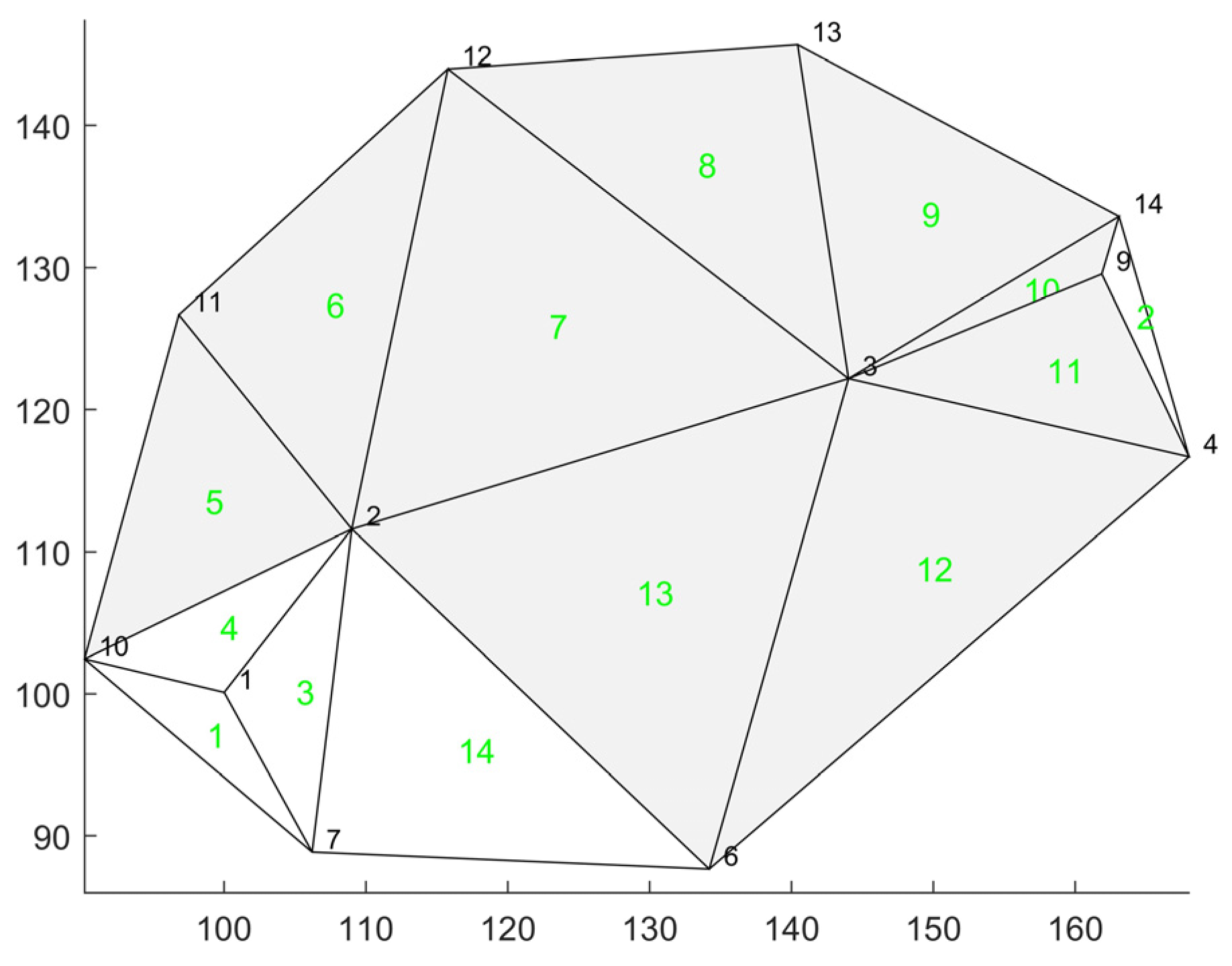
- Through the analysis in the first geometry of the geodetic network, we found that no statistically significant deformations occurred between two epochs in triangles 1, 2, 3, 4, and 14. It can be concluded that the vertices of these triangles have not moved, i.e., the reference points 1, 2, 4, 6, 7, 9 and 10 and 14 (the last two are points on the dam).
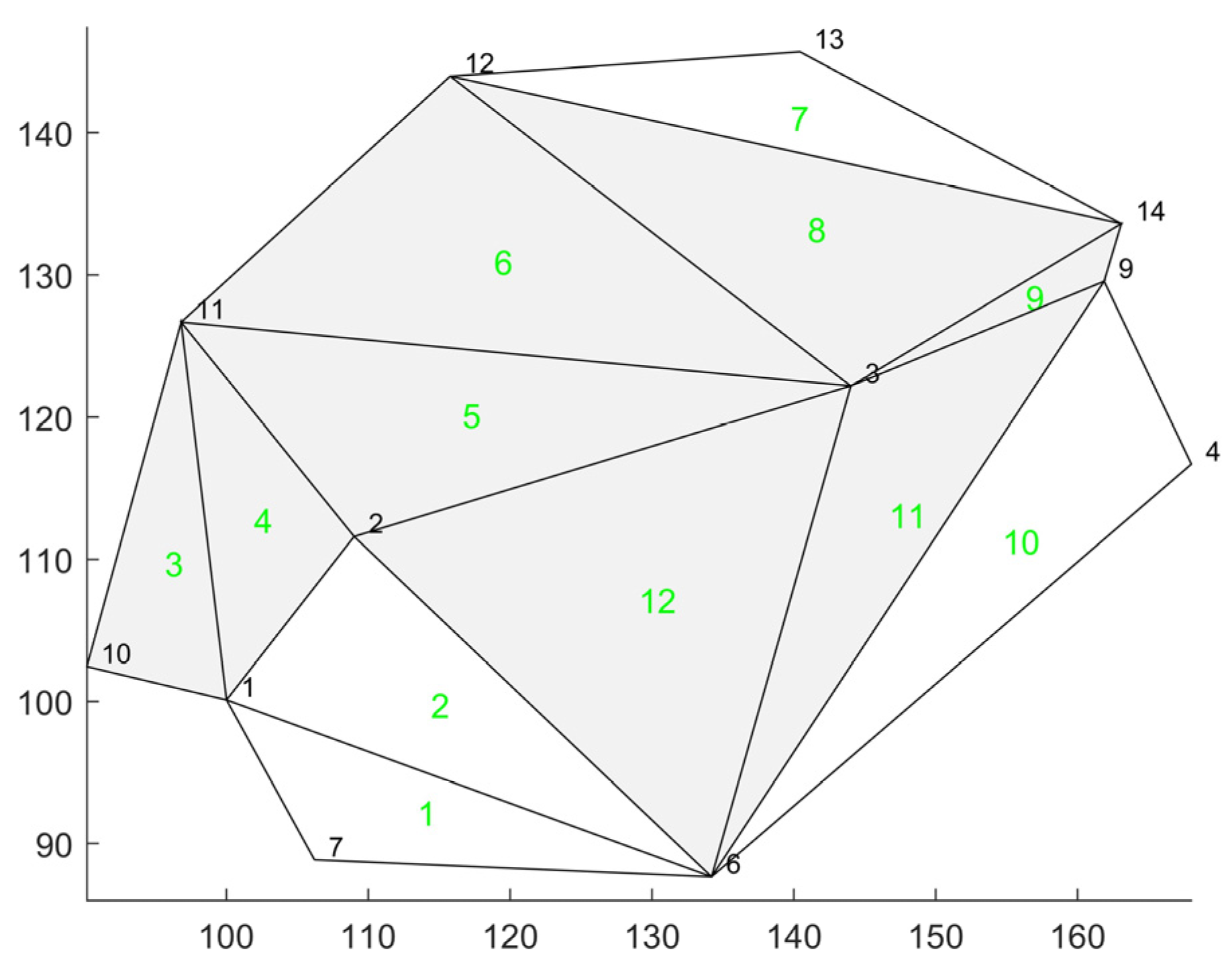
- Through the analysis in the second geometry of the geodetic network, we found that no statistically significant deformations occurred between two epochs in triangles 1, 2, 7 and 10. It can be concluded that the vertices of these triangles have not moved, i.e., the reference points 1, 2, 4, 6, 7, 9, and 12, 13 and 14 (the last three are points on the dam).
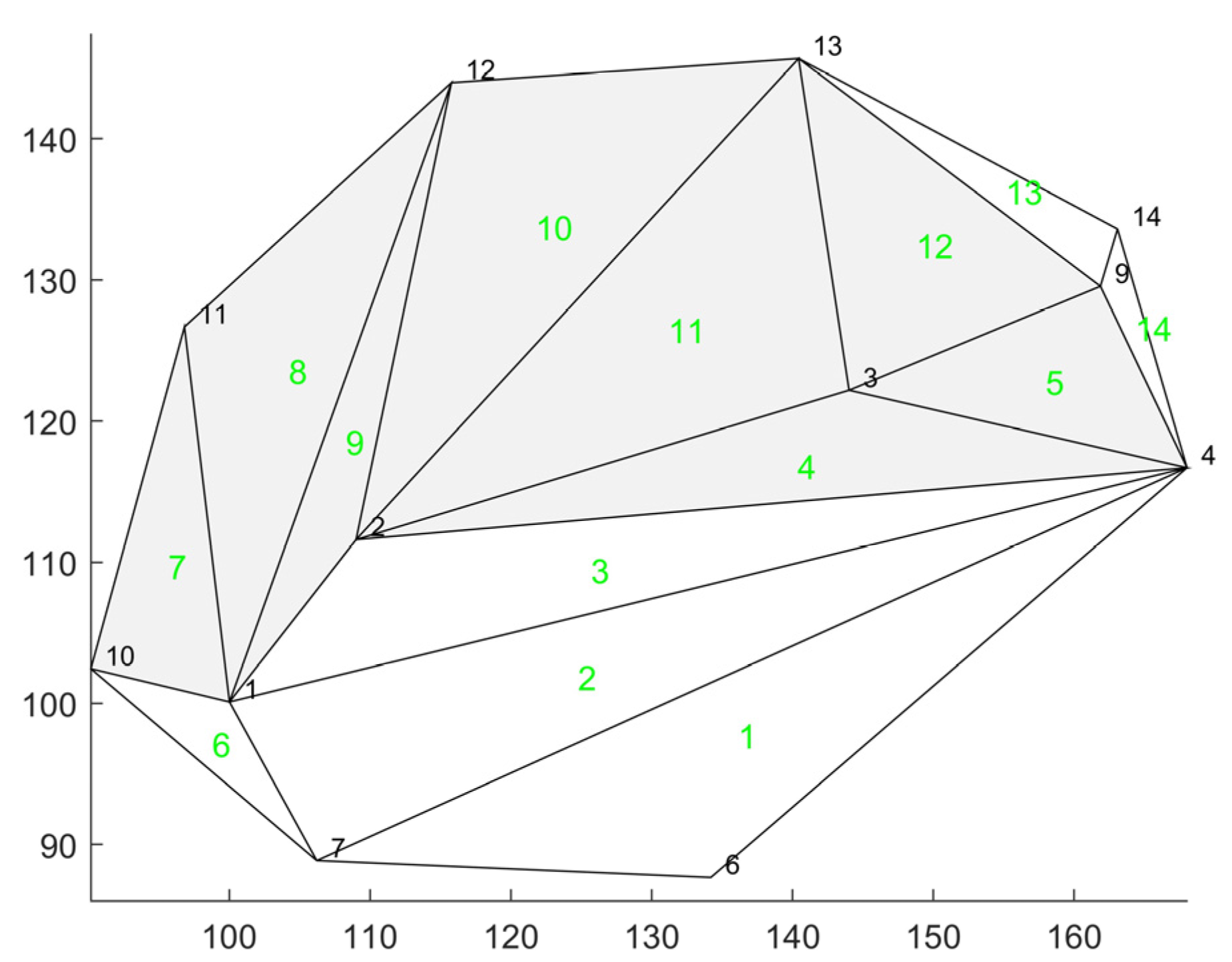
- Through the analysis in the third geometry of the geodetic network, we found that no statistically significant deformations occurred between two epochs in triangles 1, 2, 3, 6, 13 and 14. It can be concluded that the vertices of these triangles have not moved, i.e., the reference points 1, 2, 4, 6, 7, 9 and 10, 13 and 14 (the last three are points on the dam).
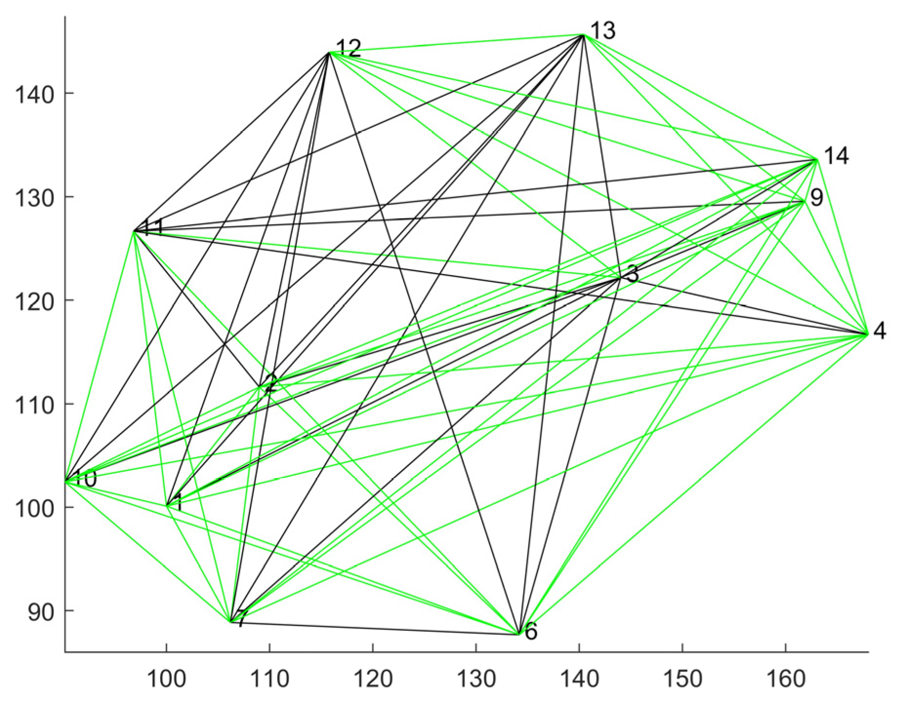
- The distances between reference points 1–2, 1–4, 1–6, 1–7, 1–9, 2–4, 2–6, 2–7, 2–9, 4–6, 4–7, 4–9, 6–9, and 7–9 have not changed in a statistically significant way. However, all distances between reference point 3 and the other reference points 3–1, 3–2, 3–4, 3–6, 3–7, and 3–9 have changed in a statistically significant manner. This analysis confirms the results of the individual triangle transformation testing that reference points 1, 2, 4, 6, 7, and 9 have not moved significantly, and that point 3 has. Only the distance between reference points 6–7 has changed in a statistically significant way (since the movements of these two points point to each other).
- Considering the pairs between the reference points (1, 2, 4, 6, 7, and 9) and the points on the dam (10 and 14) that have not moved as a result of the congruence test, we find that all distances between pairs 1–10, 1–11, 1–14, 2–10, 2–14, 4–10, 4–14, 6–10, 6–11, 6–14, 7–10, 7–11, 7–14, 9–10, 9–14 have not statistically significantly changed. The distances between the reference points and the points on the dam 1–12, 1–13, 2–12, 2–13, 3–13, 6–12, 6–13, 7–12 and 7–13 have changed statistically significantly. All of the above changes confirm the findings from testing the transformation of the individual triangle that reference points 1, 2, 4, 6, 7, and 9 have not moved significantly, and that point 3 has. Distances between 2–11, 3–10, 3–14, 4–11, and 9–11 show a statistically significant change as the points of the pair move toward each other; the distances between pairs 3–11, 3–12, 4–12, 4–13, 9–12, 9–13 do not show a statistically significant change as the two points of the pair have moved in a similar direction relative to each other.
- The distances between the points on the dam 10–11, 10–13, 10–14, 12–13, 12–14, 13–14 have not changed in a statistically significant way. The reason for this assertion is that at least one point of the listed pairs moved a little or the directions of their movement were similar. The distances between the points on dam 10–12, 11–12, 11–13, and 11–14 changed in a statistically significant way.
5. Conclusions
Author Contributions
Funding
Data Availability Statement
Conflicts of Interest
References
- Heck, B.; Kok, J.J.; Welsch, W.M.; Baumer, R.; Chrzanowski, A.; Chen, Y.Q.; Secord, J.M. Report of the FIG-working group on the analysis of deformation measurements. In 3rd International Symposium on Deformation Measurements by Geodetic Methods; Joó, I., Detreköi, A., Eds.; Akademiai Kiadó: Budapest, Hungary, 1983; pp. 337–415. [Google Scholar]
- Pelzer, H. Zur Analyse Geodätischer Deformationsmessungen; Deutsche Geodätische Kommission: München, Germany, 1971. [Google Scholar]
- Niemeier, W. Deformationsanalyse. In Geodätische Netze in Landes- und Ingenieurvermessung II; Pelzer, H., Ed.; Konrat Wittwer: Stuttgart, Germany, 1985; pp. 559–623. [Google Scholar]
- Chrzanowski, A.; Chen, Y.Q.; Secord, J.M. A Generalized Approach to the Geometrical Analysis of Deformation Surveys. In 3rd International Symposium on Deformation Measurements by Geodetic Methods; Joó, I., Detreköi, A., Eds.; Akademiai Kiadó: Budapest, Hungary, 1982. [Google Scholar]
- Chen, Y.Q. Analysis of Deformation Surveys—A Generalized Approach; Department of Geodesy and Geomatics Engineering, University of New Brunswick: Fredericton, NB, Canada, 1983. [Google Scholar]
- Chrzanowski, A.; Chen, Y.Q.; Secord, J.M. On the strain analysis of tectonic movements using fault crossing geodetic surveys. Tectonophysics 1983, 97, 297–315. [Google Scholar] [CrossRef]
- Heck, B. Das Analyseverfahren des Geodätischen Instituts der Universität Karlsruhe Stand 1983. In Deformationsanalysen ’83, Geometrische Analyse und Interpretation von Deformationen Geodätischer Netze; Schriftenreihe: München, Germany, 1983; pp. 153–182. [Google Scholar]
- Heck, B.; Kuntz, E.; Meier-Hirmer, B. Deformationsanalyse mittels relativer Fehlerellipsen. AVN 1977, 84, 78–87. [Google Scholar]
- Welsch, W. Einige Erweiterungen der Deformationsermitlung in geodätischen Netzen durch Methoden der Strainanlyse. In 3rd International Symposium on Deformation Measurements by Geodetic Methods; Joó, I., Detreköi, A., Eds.; Akademiai Kiadó: Budapest, Hungary, 1982; pp. 83–97. [Google Scholar]
- Kuang, S. Geodetic Network Analysis and Optimal Design: Concepts and Applications; Ann Arbor Press: Chelsea, MI, USA, 1996. [Google Scholar]
- Baarda, W. S-Transformations and Criterion Matrices; Computing Centre of the Delft Geodetic Institute: Delft, The Nederland, 1981. [Google Scholar]
- Welsch, W.M. Finite Element Analysis of Strain Patterns from Geodetic Observations Across a Plate Margin. In Developments in Geotectonics; Vyskočil, P., Wassef, A.M., Green, R., Eds.; Elsevier: Amsterdam, The Netherlands, 1983; pp. 57–71. [Google Scholar] [CrossRef]
- Welsch, W.; Zhang, Y. Einige Methoden zur Untersuchung kongruenter und affiner Beziehungen in geodätischen Überwachungsnetzen zur Ermittlung von Deformationen. In Deformationsanalysen’83, Geometrische Analyse und Interpretation von Deformationen Geodätischer Netze; Schriftenreihe: Munich, Germany, 1983; pp. 299–328. [Google Scholar]
- Hunter, J.J. Generalized inverses and their application to applied probability problems. Linear Algebra. Appl. 1982, 45, 157–198. [Google Scholar] [CrossRef]
- Welsch, W.M. Description of Homogeneous Horizontal Strains and some Remarks to their Analysis. In Geodetic Activities, Juneau Icefield, Alaska, 1981–1996; Welsch, W.M., Lang, M., Miller, M.M., Eds.; Schriftenreihe: Munich, Germany, 1997; pp. 73–90. [Google Scholar]
- Caspary, W.F. Concepts of Network and Deformation Analysis; School of Geomatic Engineering: Sydney, Australia, 2000. [Google Scholar]
- Nowel, K. Robust M-Estimation in Analysis of Control Network Deformations: Classical and New Method. J. Surv. Eng. 2015, 141, 04015002. [Google Scholar] [CrossRef]
- Nowel, K. Squared Msplit(q) S-transformation of control network deformations. J. Geod. 2018, 93, 1025–1044. [Google Scholar] [CrossRef]
- Batilović, M.; Kanović, Ž.; Sušić, Z.; Marković, M.Z.; Bulatović, V. Deformation analysis: The modified GREDOD method. Geod. Vestnik. 2022, 66, 60–75. [Google Scholar] [CrossRef]

| Method | Test Statistic | Equation | |
|---|---|---|---|
| X-method | coordinates | (4) | |
| L-method | distances | (6), (12) and (13) | |
| angles | (6), (14) and (15) | ||
| dist. + angles | (6) and (16) |
| Par. | or | Rejected? | p-Value [%] | |||||||
|---|---|---|---|---|---|---|---|---|---|---|
| Trian. | ||||||||||
| 1 | −6.44 | −16.08 | −4.88 | −0.9 | 0.002 | 0.003 | 2.35 | no | 8.20 | |
| 2 | 24.35 | 47.82 | 41.74 | −7.4 | −0.017 | −0.008 | 0.76 | no | 52.10 | |
| 3 | 0.00 | −8.81 | 0.29 | −1.8 | 0.000 | 0.002 | 0.37 | no | 77.74 | |
| 4 | 6.70 | −11.61 | −3.49 | −0.6 | 0.000 | 0.002 | 2.48 | no | 7.04 | |
| 5 | 15.97 | −28.67 | 10.89 | −3.2 | −0.001 | 0.004 | 7.41 | yes | 0.03 | |
| 6 | 42.26 | 9.18 | 64.29 | −2.1 | −0.007 | −0.007 | 14.97 | yes | 0.00 | |
| 7 | 51.37 | −3.22 | −25.33 | 4.3 | −0.003 | 0.001 | 28.59 | yes | 0.00 | |
| 8 | 66.13 | 14.39 | −6.93 | 5.6 | −0.007 | −0.005 | 7.19 | yes | 0.03 | |
| 9 | 66.03 | 15.74 | 15.08 | 6.0 | −0.007 | −0.008 | 18.93 | yes | 0.00 | |
| 10 | 50.48 | 5.36 | 33.12 | 1.9 | −0.006 | −0.007 | 6.13 | yes | 0.11 | |
| 11 | −6.28 | 14.28 | 35.43 | −1.1 | −0.003 | −0.007 | 7.63 | yes | 0.02 | |
| 12 | −19.16 | −3.02 | 28.19 | −4.0 | −0.001 | −0.002 | 11.51 | yes | 0.00 | |
| 13 | −13.18 | −7.11 | −17.09 | −0.5 | 0.002 | 0.003 | 5.80 | yes | 0.15 | |
| 14 | −0.87 | −3.88 | −22.07 | −2.3 | −0.001 | 0.004 | 2.73 | no | 5.22 | |
| Par. | or | Rejected? | p-Value [%] | |||||||
|---|---|---|---|---|---|---|---|---|---|---|
| Trian. | ||||||||||
| 1 | 4.03 | −11.50 | −22.73 | −3.9 | −0.001 | 0.006 | 2.54 | no | 6.54 | |
| 2 | −3.56 | −0.93 | −14.04 | −1.1 | 0.000 | 0.002 | 1.51 | no | 22.11 | |
| 3 | 14.24 | −22.75 | −9.23 | −3.3 | −0.001 | 0.005 | 8.60 | yes | 0.01 | |
| 4 | 13.05 | −25.81 | 22.43 | −1.9 | 0.000 | 0.001 | 3.93 | yes | 1.28 | |
| 5 | 15.76 | −34.48 | −3.18 | −4.4 | −0.001 | 0.007 | 11.84 | yes | 0.00 | |
| 6 | 72.29 | 26.38 | 7.90 | 7.1 | −0.008 | −0.009 | 14.44 | yes | 0.00 | |
| 7 | 67.14 | −2.42 | −4.61 | 2.1 | −0.007 | 0.000 | 0.89 | no | 45.41 | |
| 8 | 65.61 | 22.95 | 6.59 | 7.4 | −0.007 | −0.009 | 18.59 | yes | 0.00 | |
| 9 | 50.48 | 5.36 | 33.12 | 1.9 | −0.006 | −0.007 | 6.13 | yes | 0.11 | |
| 10 | −11.03 | 3.48 | 11.02 | −1.2 | 0.000 | −0.001 | 1.87 | no | 14.55 | |
| 11 | −21.82 | −1.61 | 51.19 | −5.7 | −0.002 | −0.005 | 8.23 | yes | 0.01 | |
| 12 | −13.18 | −7.11 | −17.09 | −0.5 | 0.002 | 0.003 | 5.80 | yes | 0.15 | |
| Par. | Ali | Rejected? | p-Value [%] | |||||||
|---|---|---|---|---|---|---|---|---|---|---|
| Trian. | ||||||||||
| 1 | −7.93 | 20.22 | −20.00 | 2.8 | 0.000 | 0.000 | 2.76 | no | 5.02 | |
| 2 | 1.43 | −6.90 | 2.53 | −2.0 | −0.001 | 0.002 | 0.99 | no | 40.40 | |
| 3 | −2.84 | −8.22 | 3.43 | −2.4 | 0.000 | 0.002 | 0.98 | no | 40.73 | |
| 4 | −55.38 | −46.14 | 10.36 | −11.2 | 0.005 | 0.010 | 14.76 | yes | 0.00 | |
| 5 | −6.28 | 14.28 | 35.43 | −1.1 | −0.003 | −0.007 | 7.63 | yes | 0.02 | |
| 6 | −6.44 | −16.08 | −4.88 | −0.9 | 0.002 | 0.003 | 2.35 | no | 8.20 | |
| 7 | 14.24 | −22.75 | −9.23 | −3.3 | −0.001 | 0.005 | 8.60 | yes | 0.01 | |
| 8 | 19.85 | 6.43 | 87.98 | −6.9 | −0.006 | −0.006 | 15.40 | yes | 0.00 | |
| 9 | 63.24 | −28.82 | −51.92 | 10.7 | 0.001 | 0.003 | 10.81 | yes | 0.00 | |
| 10 | 48.73 | 0.95 | −4.98 | 2.6 | −0.004 | −0.001 | 11.87 | yes | 0.00 | |
| 11 | 63.82 | 4.95 | −31.40 | 6.8 | −0.004 | −0.001 | 29.59 | yes | 0.00 | |
| 12 | 66.45 | 17.51 | 20.36 | 5.8 | −0.007 | −0.009 | 19.13 | yes | 0.00 | |
| 13 | 55.02 | 2.15 | 3.72 | 4.4 | −0.004 | −0.004 | 1.41 | no | 25.01 | |
| 14 | 24.35 | 47.82 | 41.74 | −7.4 | −0.017 | −0.008 | 0.76 | no | 52.10 | |
| pair | 1 | 2 | 3 | 4 | 6 | 7 | 9 | 10 | 11 | 12 | 13 | 14 |
| 1 | / | 0.63 | 16.89 | 0.03 | 3.45 | 0.23 | 0.41 | 0.01 | 2.50 | 20.38 | 9.66 | 0.00 |
| 2 | / | 15.80 | 0.23 | 1.75 | 0.05 | 0.00 | 0.45 | 6.89 | 25.58 | 14.75 | 0.37 | |
| 3 | / | 11.69 | 8.94 | 16.96 | 14.74 | 6.55 | 0.31 | 0.62 | 20.49 | 16.46 | ||
| 4 | / | 0.82 | 0.49 | 0.48 | 0.04 | 7.01 | 1.04 | 3.90 | 0.00 | |||
| 6 | / | 7.03 | 0.04 | 1.13 | 2.11 | 8.04 | 9.26 | 0.27 | ||||
| 7 | / | 1.18 | 0.55 | 3.38 | 15.99 | 8.10 | 0.12 | |||||
| 9 | / | 0.28 | 5.73 | 0.05 | 3.54 | 1.35 | ||||||
| 10 | / | 0.01 | 12.52 | 4.28 | 0.01 | |||||||
| 11 | / | 38.65 | 22.36 | 6.92 | ||||||||
| 12 | / | 0.21 | 0.00 | |||||||||
| 13 | / | 1.60 | ||||||||||
| 14 | / |
| Par. | ||||||||
|---|---|---|---|---|---|---|---|---|
| Triangle | ||||||||
| 1 | −11.32 | 10.44 | −21.76 | 16.10 | −32.16 | 43 | 88 | |
| 2 | 66.09 | 81.65 | −15.57 | 48.61 | 95.65 | 140 | 5 | |
| 3 | 0.29 | 8.96 | −8.67 | 8.81 | −17.62 | 44 | 89 | |
| 4 | 3.20 | 14.28 | −11.08 | 12.68 | −23.23 | 147 | 12 | |
| 5 | 26.86 | 42.21 | −15.35 | 28.78 | −57.33 | 138 | 3 | |
| 6 | 106.55 | 67.62 | 38.94 | 14.34 | 18.37 | 160 | 25 | |
| 7 | 26.04 | 51.50 | −25.46 | 38.48 | −6.44 | 178 | 43 | |
| 8 | 59.20 | 68.86 | −9.67 | 39.27 | 28.79 | 10 | 55 | |
| 9 | 81.11 | 70.50 | 10.61 | 29.95 | 31.48 | 16 | 61 | |
| 10 | 83.60 | 52.00 | 31.60 | 10.20 | 10.71 | 16 | 61 | |
| 11 | 29.15 | 39.85 | −10.70 | 25.27 | 28.55 | 163 | 28 | |
| 12 | 9.03 | 28.38 | −19.35 | 23.87 | −6.05 | 3 | 48 | |
| 13 | −30.27 | −7.76 | −22.50 | 7.37 | −14.21 | 143 | 8 | |
| 14 | −22.94 | −0.18 | −22.76 | 11.29 | −7.77 | 170 | 35 | |
Disclaimer/Publisher’s Note: The statements, opinions and data contained in all publications are solely those of the individual author(s) and contributor(s) and not of MDPI and/or the editor(s). MDPI and/or the editor(s) disclaim responsibility for any injury to people or property resulting from any ideas, methods, instructions or products referred to in the content. |
© 2023 by the authors. Licensee MDPI, Basel, Switzerland. This article is an open access article distributed under the terms and conditions of the Creative Commons Attribution (CC BY) license (https://creativecommons.org/licenses/by/4.0/).
Share and Cite
Ambrožič, T.; Turk, G.; Marjetič, A. Geodetic Applications and Improvement of the X- and L-Method of Deformation Analysis. Geosciences 2023, 13, 330. https://doi.org/10.3390/geosciences13110330
Ambrožič T, Turk G, Marjetič A. Geodetic Applications and Improvement of the X- and L-Method of Deformation Analysis. Geosciences. 2023; 13(11):330. https://doi.org/10.3390/geosciences13110330
Chicago/Turabian StyleAmbrožič, Tomaž, Goran Turk, and Aleš Marjetič. 2023. "Geodetic Applications and Improvement of the X- and L-Method of Deformation Analysis" Geosciences 13, no. 11: 330. https://doi.org/10.3390/geosciences13110330
APA StyleAmbrožič, T., Turk, G., & Marjetič, A. (2023). Geodetic Applications and Improvement of the X- and L-Method of Deformation Analysis. Geosciences, 13(11), 330. https://doi.org/10.3390/geosciences13110330