1. Introduction
Bedrock rivers [
1] carve their paths through solid rock formations, exhibiting distinctive morphological and hydrological characteristics. Bedrock rivers, formally defined as those where a significant portion of the land–river interface boundary consists of exposed bedrock [
2], are characterized by a transport capacity within the channel that exceeds the quantity of sediment transported to the river [
3]. Unlike alluvial rivers, bedrock rivers directly incise into the underlying bedrock, playing a pivotal role in shaping landscapes over geological timescales [
4]. While most environmental studies on riverine geochemistry focus on alluvial rivers, where the channel bed and bank materials consist of loose unconsolidated sediments, the geochemistry of bedrock rivers remains relatively understudied.
Certain trace elements, such as Cu, Pb, or Sn, have been intimately associated with human activities since the dawn of civilization [
5]. Particularly, the advent of industrialization and the mid-20th century’s “Great Acceleration” [
6] has triggered an unprecedented release of trace elements into the environment. Despite the mitigation efforts through environmental protection policies and measures [
7], these elements continue to pose potential risks to ecosystems and human health, often referred to as industrial metals [
8], risk elements [
9], or potentially toxic elements [
10]. Elements like Cr, Cu, Hg, Ni, Pb, and Zn in the urban environment [
11] are pivotal indicators for understanding human–nature relationships. Their study in urban effluents is critical for assessing water protection and waste management policies [
12].
Environmental assessments of fluvial sediments often involve anthropogenic elements naturally present in the environment. To distinguish the natural and non-natural sources contributing to the sediment composition, differentiating geochemical signals [
13] that may cause composition variability is imperative. Concerning natural contents (i.e., “amount-of-substance of a component divided by the mass of the system” [
14]), it is widely acknowledged that the chemical composition of the source rock and the particle-size distribution significantly contribute to the natural variation in sediment composition [
15], hindering the identification of human inputs.
To discern anthropogenic contributions, normalization is a common practice for minimizing the effects of natural variability in order to discern anthropogenic contributions [
16]. Many authors concur that among the natural controlling factors influencing sediment content variability [
16,
17,
18], particle size plays a pivotal role. To mitigate the particle-size effect, the separation of the fine fraction (particle size <0.063 mm) is the most common physical normalization method [
19]. However, some researchers argue that size normalization through the exclusion of the fine fraction can introduce bias due to the omission of minerals that can substantially influence trace element sediment contents [
3,
9]. Some studies also report that fine-grained sediments from bedrock rivers have a limited influence on the trace element composition [
3,
20].
Numerous techniques have been developed for estimating background values [
21] and identifying content values that significantly deviate from the natural reference (enrichments). With the aim of improving background estimation and achieving a more precise identification of enrichments, this study presents a comparative analysis between two commonly used particle-size fractions: the <2 mm fraction, containing sand, silt, and clays (gravels were excluded from samples), and the fine fraction (<0.063 mm). A site-specific investigation is conducted to discern the differences and similarities between these two fractions.
2. Materials and Methods
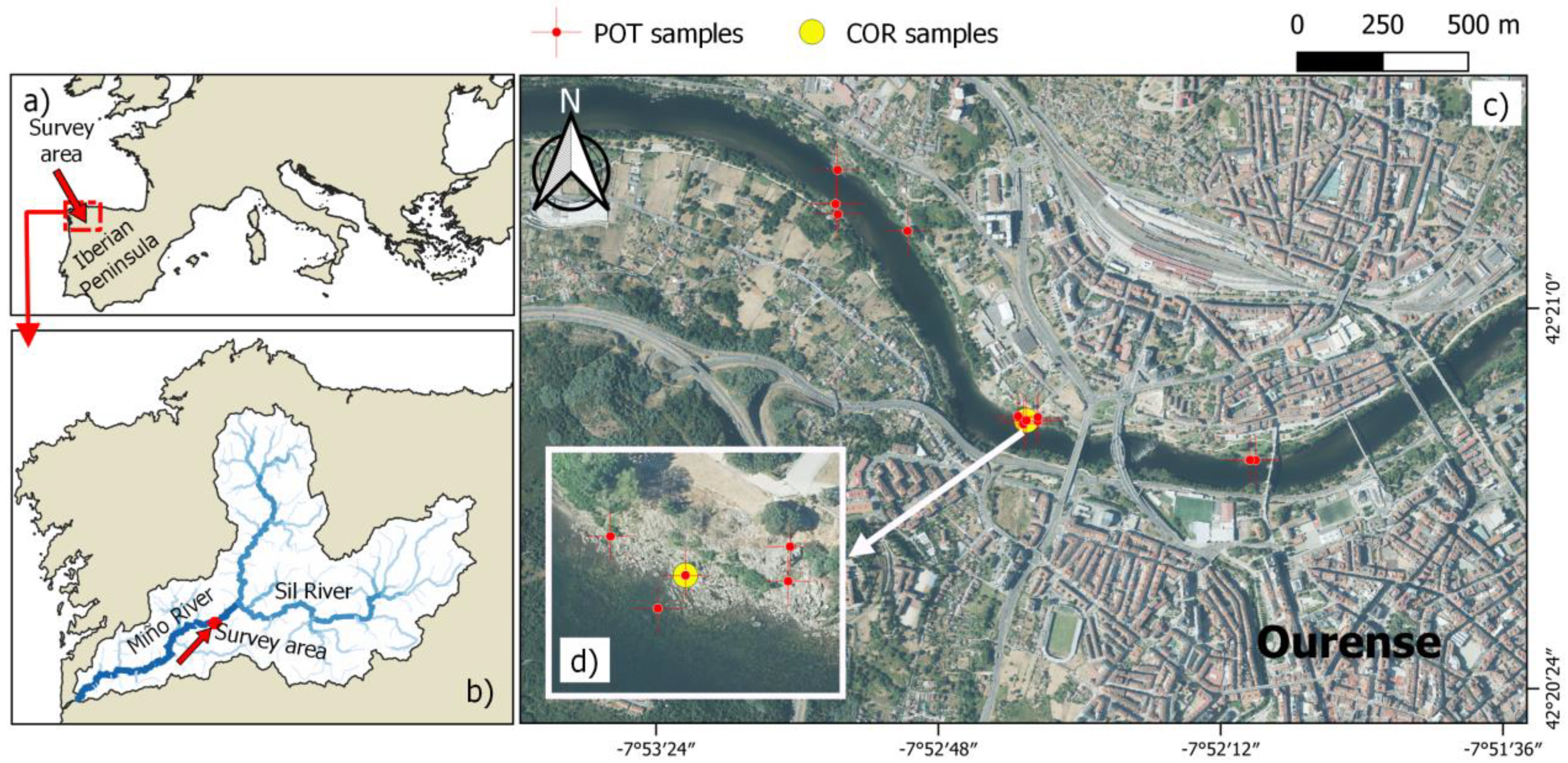
2.1. Surveyed Area
The Miño River (Minho in Portuguese) constitutes a major watercourse within the NW Iberian Massif, located in the Iberian Peninsula. Stretching over a length of 315 km, it flows through a drainage area encompassing approximately 17,619 km
2 [
22], alongside its principal tributary, the Sil River. Due to the importance of this tributary, it is often referred to as the Miño-Sil system or the Miño-Sil River. This system sustains an annual average flow of 340 m
3 s
−1 (from 2011 to 2019, [
23]), ultimately discharging its waters into the Atlantic Ocean. The final 78 km of its course delineate the border between Spain and Portugal.
This study was conducted in a mid-urban stretch of the river as it courses through the town of Ourense in Spain, following an east–west direction. The study area encompasses a 2 km segment of a bedrock channel characterized by siliceous materials, predominantly consisting of alkaline granitoids, granodiorites, schists, and Quaternary deposits (old fluvial terraces) [
24]. At this location, the river maintains an average elevation of 100 m a.s.l., a very gentle water mass gradient of 0.07%, and an annual average flow (2010–2019) of 244 m
3 s
−1 [
23]. The annual total precipitation ranges between 500 and 1000 mm, with a pronounced decline in summer (2012–2020). The monthly average temperature varies from 5 to 25 °C, with an annual average of 15 °C (2011–2020 [
25]).
Human activities have significantly transformed the surveyed river stretch, as shown in
Figure 1. The municipality of Ourense falls under Eurostat’s classification [
26] of “cities” (with at least 50% of the population residing in urban centers), according to the degree of urbanization (DEGURBA). Its immediate urban vicinity boasts a population density of approximately 1240 inhabitants per km
2 [
27]. Significant alterations relevant to this stretch are closely associated with dams that regulate water flow and alter base levels. Upstream, the Velle dam, constructed in 1966, has a capacity of 17 hm
3. Downstream, the Castrelo de Miño dam, built in 1969, possesses a capacity of 60 hm
3 [
28]. Both dams are utilized for hydroelectric power generation. Additionally, the presence of bridges interconnecting urban zones, promenades, and structures, along with the area’s notable thermal springs, attracts both locals and tourists to thermal facilities.
2.2. Sample Collection and Processing
Sampling was conducted in two distinct campaigns. In the first campaign, a total of 12 samples were acquired from surface sediments (0–5 cm) confined within potholes and other rock cavities, hereafter referred to as POT samples. These cavities were strategically located along the riverbank in areas commonly submerged, and the sampling took place during a period of low flow in the summer season. In the subsequent campaign, a profile reaching a depth of 24 cm was collected from within a pothole (COR samples). This profile was subsequently divided into 2 cm intervals. The collected samples underwent oven drying at a temperature of 45 ± 5 °C until a constant weight was achieved. Following drying, the samples were subjected to sieving through 2 mm and 0.063 mm sieves to separate the <2 mm fraction (referred to as F2) and the <0.063 mm fraction (referred to as F63), respectively.
2.3. Determination of Sediment Composition
The samples were commissioned to the Center for Scientific-Technological Research Support (CACTI-UVigo), an ISO 9001-certified laboratory [
31], for compositional analysis. The <2 mm fraction was analyzed using X-ray fluorescence, while the <0.063 mm fraction, due to its limited quantity, underwent analysis using optical emission inductively coupled plasma spectrometry (ICP-OES). The chosen target elements for the analysis included As, Cr, Cu, Ni, Pb, and Zn, as these elements are commonly associated with human activities. Additionally, Al, Ca, Fe, Rb, and Y were selected as reference elements. Aluminum and Fe were chosen as reference elements due to their widespread use [
32]. Rb was recommended as a reference element for sediment normalization by [
33]. Calcium was selected to represent minor constituents in source rocks, and Y was chosen based on its demonstrated effectiveness in previous studies involving the normalization of rare earth elements in the region [
34]. However, an initial assessment of the data raised concerns regarding a significant non-natural enrichment of Fe, particularly in the core sediments within a pothole (up to 12% in the COR12 sample). Additionally, during the sampling process, the presence of red coloring attributed to iron-debris, i.e., construction and demolition waste dumped in the river in the past, was evident at the base of the cavity, indicating oxidation. Consequently, Fe was excluded as a reference element due to its potential to violate the requirement that reference elements should not be significantly affected by human sources [
16].
2.4. Data Treatment
The compositional data analysis was conducted using Statgraphics Centurion 18 software (©Statgraphics Technologies, Inc., The Planins, VA, USA). In the initial exploratory data analysis, robust non-parametric methodologies were preferred. While a normal distribution is typically assumed for natural compositions, factors such as diverse lithologies or contamination can introduce deviations from normality. Therefore, non-parametric statistical techniques were deemed more suitable for the preliminary analysis. In this context, the Kruskal–Wallis test was employed to identify differences and similarities between subsets, and Tukey inner fences were utilized to identify outliers. Outliers were defined as values falling outside the range determined by Q1 − 1.5IQR to Q3 + 1.5IQR, where IQR represents the interquartile range between the first quartile (Q1, 25th percentile) and the third quartile (Q3, 75th percentile).
Parametric statistics were selectively applied only to subsets exhibiting confirmed normal distribution characteristics. For instance, least-squares simple regression was employed to model background functions. Background estimation involved the use of background functions [
9,
21], established by regressing the content of a specific target element (dependent variable, y-coordinate) against that of a reference element (independent variable, x-coordinate). Least-squares simple regression facilitated the calculation of the background as a linear function (BGf), as illustrated in Equation (1):
where [TE]
BG represents the theoretical background content of a specific target element (TE) calculated based on the content of a reference element (RE), “a” denotes the slope of the function and “b” indicates the intercept. It is important to note that this approach was undertaken after confirming that deviations from normality within the dataset could be attributed to identifiable outliers (further details on this will be provided in the results section).
After deriving the background functions (BGfs), the subsequent assessment was conducted through enrichment factor (EF) analysis [
35]. As the BGfs were computed using data from the study’s dataset and the reference element was obtained from the same study area, the term “local enrichment factor” (LEF) is employed here. The LEFs were calculated using Equation (2):
where [TE] represents the measured content of the designated target element (TE).
The Local Enrichment Factor (LEF) is calculated for each sample and varies based on the content of the reference element (RE). Various criteria have been employed to define contamination. In this study, the assessment relies on the term “enrichment” (when measured values exceed expected levels), and thresholds are determined through the LEF, the empirical rule (one-tail normal distribution), and the average and relative standard deviation (RSD = SD/mean) of background samples (those involved in the background function). The empirical rule was selected because it is a statistical guideline that describes the approximate percentage of data values falling within certain standard deviation intervals of a normal distribution. This approach enables classification into four categories:
Background: LEFs below the threshold of 1 + RSD. Theoretically, any value within the normal mode (background) has an 84% probability of falling below this threshold (one-tail normal distribution). The probability of belonging to a different population (enrichment) is below 26%.
Negligible/Suspected Enrichment: LEFs ranging between 1 + RSD (84% probability) and 1 + 2RSD (97.5% probability). Values within this range have a 13.5% probability of belonging to the normal (background) mode, indicating an 86.5% potential for enrichment.
Probable Enrichment: LEFs between 1 + 2RSD and 1 + 3RSD. This range encompasses only 2.35% of the normal (background) mode, resulting in a 97.65% likelihood of being from a different population.
Secure Enrichment: LEFs exceeding 1 + 3RSD, a limit encompassing 99.85% of conceivable values within the normal (background) mode. Thus, the probability of any value exceeding this threshold and belonging to the background population is less than 0.15%.
Importantly, it is essential to emphasize that enrichment does not inherently indicate risk or harm; rather, it serves as a gauge of potential human-induced contributions to sediment composition, thereby facilitating functions such as contamination identification and tracing. Risk assessment lies beyond the scope of this study.
3. Results and Discussion
The surveyed area encompasses a bedrock river characterized by the prevalent exposure of boulders, cobble, and pebbles, which constitute widespread and dominant components of the sediment. During the sampling process, materials exceeding 5 cm in size were excluded. The remaining sediments underwent particle size analysis, revealing the following median distributions: 29.2% gravel (>2 mm), 47.6% sands (ranging between 2 and 0.063 mm), and 0.5% fines (<0.063 mm). It is noteworthy that the fine fraction was notably limited, accounting for 0.2% to 5.9% of the dry weight.
3.1. Preliminary Data Analysis
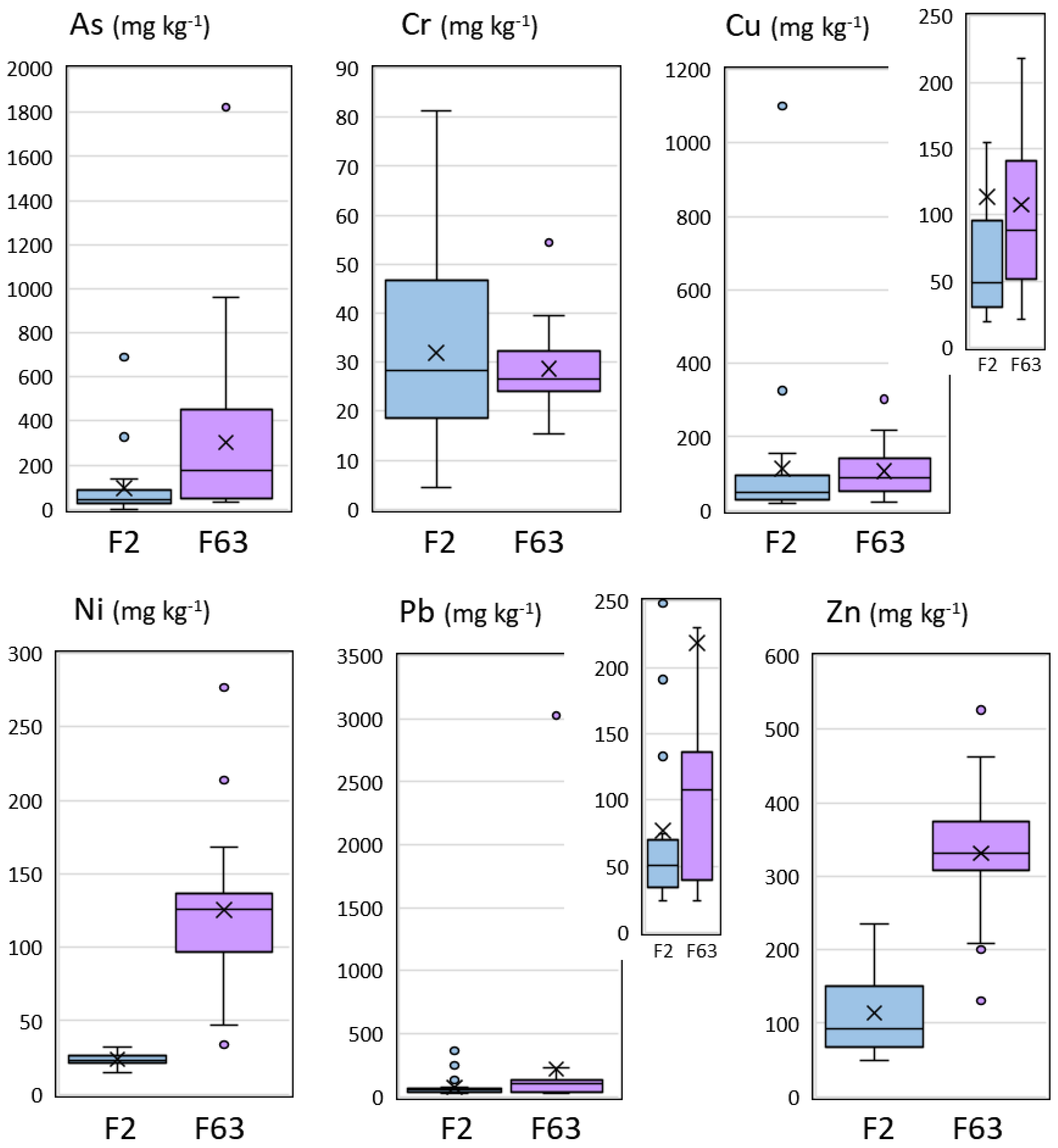
Table 1 provides a summarized overview of the elemental composition of the samples. The initial analysis focused on exploring similarities and disparities between the contents of the two analyzed fractions, namely, <2 mm (F2) and <0.063 mm (F63). This investigation employed two distinct methods to evaluate the similarities and differences within the datasets. First, an F-Test (ANOVA) was utilized to discern any significant disparities among the means, maintaining a 5% significance level. Concurrently, a Kruskal–Wallis test was employed to compare the medians with a 95% confidence level.
The results from both tests indicated that only As, Ni, and Zn exhibited statistically significant differences (
p-value < 0.05) between the fractions. Notably, these differences suggest an enrichment trend within the fine fraction (F63), as depicted in
Figure 2 and detailed in
Table 1. While Cu and Pb displayed apparent differences in medians that also suggested enrichment within the fine fraction, no statistically significant differences were observed in these cases. It is worth highlighting that the element Cr appears to demonstrate a consistent presence regardless of the size-fraction.
Regarding data normality, it is worth noting that only Cr (within the F2 fraction), as well as Ni and Zn (in both the F2 and F63 fractions), exhibited standardized skewness and kurtosis values within the range of −2 to +2. An iterative process was employed, involving the removal of outliers according to Tukey’s inner fences, until no outliers remained within the dataset; the majority of samples remained (with a maximum of six outliers for As in the F2 fraction). In general, across all elements, the subset devoid of outliers displayed standardized skewness and kurtosis well within the range consistent with a normal distribution (+2 to −2). There were only two exceptions with slightly elevated standardized skewness values, namely, As (within F63), with a value of 2.1, and Cu (within F2), with a value of 2.2. Overall, it can be inferred that the majority of the data adhered to a normal distribution, with departures from normality attributed to a limited number of easily identifiable instances.
3.2. Estimation of the Background
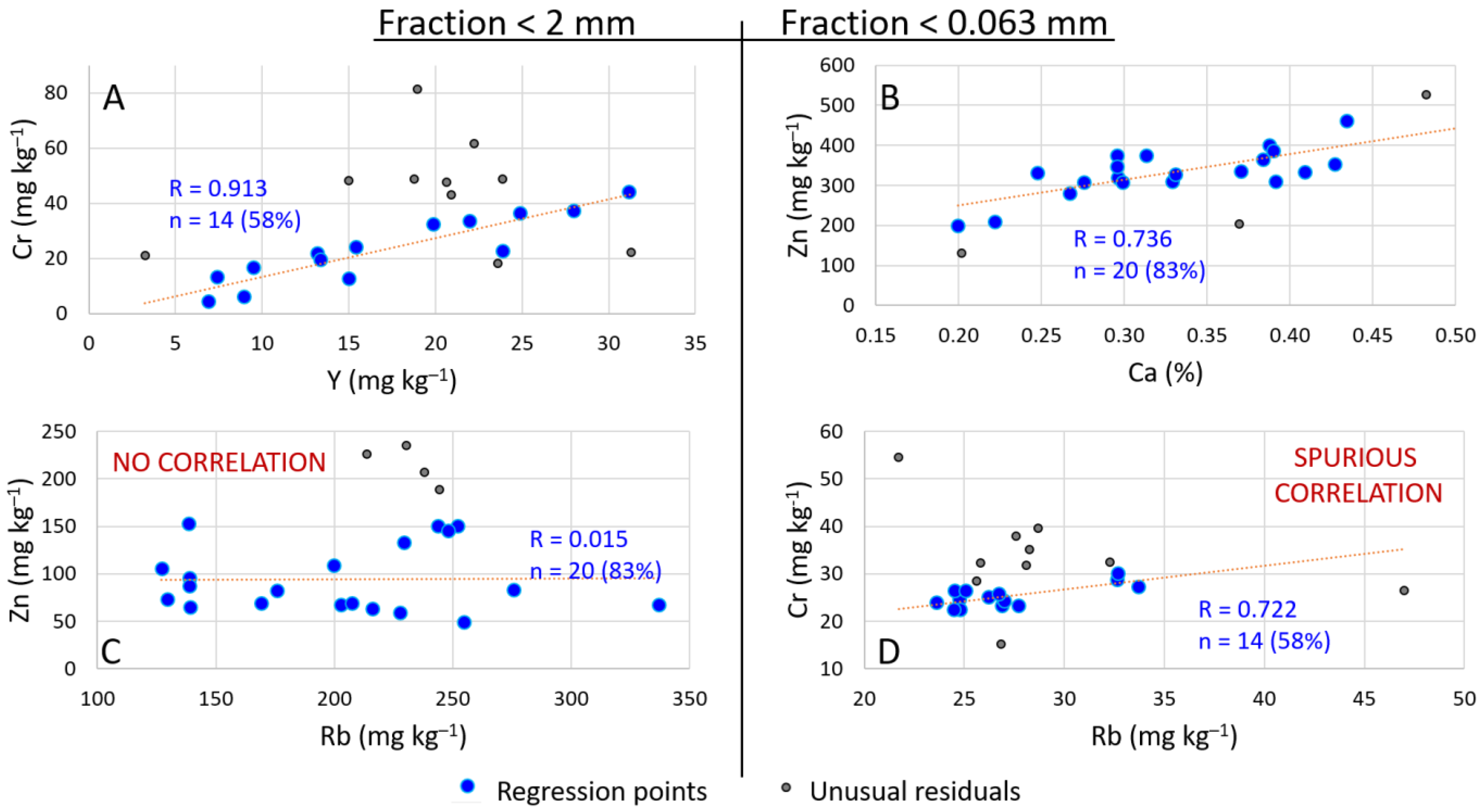
Assuming a normal distribution of background contents for target elements (as estimated by the subset devoid of outliers), background functions were computed using iterative least-squares regression. This process involved regressing the target element (dependent variable) against a specific reference element (independent variable) iteratively. Unusual residuals (Studentized residuals greater than 2) were progressively excluded in each iteration, repeating until no such unusual residuals remained within the model. The selection of background functions was based on the following criteria: (i) a correlation coefficient (R) greater than 0.5, (ii) the presence of a number of samples within the regression model (after the iterative removal of unusual residuals) exceeding 50% of the dataset, and (iii) the scrutiny of bi-plots (TE vs. RE) to avoid spurious correlations [
15].
Figure 3 illustrates graphical representations of selected examples from the iterative least squares correlation outputs. The complete analysis, along with the database, has been included as
supplementary material. It is crucial to exercise caution when employing this approach for background estimation, as highlighted in previous research [
13]. Specifically,
Figure 3D provides a clear example, where the correlation between Cr (dependent variable) and Rb (independent variable) displays a respectable correlation coefficient of 0.722 and a reasonable number of samples (14, equivalent to 58% of the dataset). However, the distribution depicted in the plot exhibits characteristics that could be interpreted as bi-modal or indicative of the summation of two distinct populations. Consequently, this observation raises questions about the validity of using least squares regression, which assumes data normality. The resulting background functions derived from this methodology are detailed in
Table 2.
The background function serves as an empirical representation of the potential background that each sample can exhibit based on its association with a reference element. Furthermore, the background content can be estimated from the samples included in the regression. Thus, the background population can be statistically characterized by its mean and standard deviation (SD), as detailed in
Table 2.
The sediment samples under study generally exhibit elevated contents compared to various references (
Table 1) on a global scale (UCC, [
36]), in regional contexts (Galician sedimentary soils, [
38]), and even in comparison with the composition of local granites [
37]. This disparity is particularly pronounced in the <0.063 fraction, as expected due to the fine fraction’s tendency to concentrate trace elements. An exception is observed with Cr, where the estimated background contents remain consistent across fractions (
Table 1), resembling the contents found in Galician sedimentary soils and local granites and falling below the global reference of the upper continental crust.
The presence of granitic rock formations, along with associated mineralization (often associated with granitic rock formations), and the influence of regional geological structures such as faults and folds could potentially create favorable conditions for the concentration of trace elements. Additionally, it is essential to acknowledge that the samples originate from potholes and other rock cavities, which experience inundation during the wet season and subsequent evaporation in the summer. This phenomenon can facilitate the precipitation of dissolved solids and the development of authigenic secondary minerals like Fe and Mn oxyhydroxides, capable of capturing trace elements [
39]. It is also prudent to consider the impact of the region’s geothermal activity and hydrothermal systems, which may contribute to the occurrence of these elements [
40]. The surveyed urban stretch of the Miño River in this study has reported up to 39 thermal springs [
41]. Furthermore, prior investigations have identified the enrichment of actinoids (particularly Th) in sediments, potentially linked to hydrothermal activity in the area [
42]. It is essential to emphasize that this assessment remains speculative in nature, and further research is warranted to unravel the true controlling factors and their impact on sediment composition.
3.3. Thresholds
When evaluating the significance of enrichment factors, it is common to apply a classification scheme to distinguish between enrichment and background levels. Various researchers have proposed distinct classification criteria for this purpose.
For instance, Hakanson [
43] introduced a classification for contamination factors (Cf), consisting of four levels: Cf <1 indicating low contamination, 1 ≤ Cf < 3 reflecting moderate contamination, 3 ≤ Cf < 6 representing considerable contamination, and Cf ≥6 signifying very high contamination. Yongming et al. [
44] established a classification with five levels for enrichment factors (EF): EF <2 denoting deficiency to minimal enrichment, 2 ≤ EF < 5 indicating moderate enrichment, 5 ≤ EF < 20 representing significant enrichment, 20 ≤ EF < 40 reflecting very high enrichment, and EF >40 characterizing extremely high enrichment. Mora et al. [
45] simplified Hakanson’s criterion [
43] for normalized enrichment factors (NEFs), categorizing as follows: NEF ≤2 suggests negligible to low contamination, 2 < NEF ≤ 3 denotes moderate contamination, and NEF >3 indicates certain to severe contamination. More recently, Li et al. [
46] introduced a classification with six levels: EF <1.5 signifies no enrichment, 1.5 ≤ EF < 2 suggests slight enrichment, 2 ≤ EF < 5 indicates moderate enrichment, 5 ≤ EF < 20 reflects severe enrichment, 20 ≤ EF < 40 denotes highly severe enrichment, and EF ≥40 characterizes extremely severe enrichment. Birch [
35] also proposed a six-level classification scheme: EF <1.5 for no enrichment, 1.5 < EF < 3.0 for slight enrichment, 3.0 < EF < 5.0 for moderate enrichment, 5.0 < EF < 10 for substantial enrichment, 10 < EF < 25 for high enrichment, and EF >25 for severe enrichment.
The application of automatic arbitrary thresholds for the environmental assessment of enrichment factors has its limitations. A lack of uniform criteria can lead to a variability of outcomes when utilizing the same dataset [
35]. Furthermore, these criteria often generalize and do not account for the unique characteristics of the studied area. Matys Grygar and Popelka [
9] propose considering percentiles or thresholds derived from the uncertainty of regression, addressing the need for a more tailored approach.
Another common error is equating enrichment with contamination, despite their non-synonymous nature. An example from a previous study in the Artabro Gulf [
47] demonstrated elevated Cr, Ni, and V contents in a small river draining into the gulf, attributed to local lithology rather than contamination. This underscores the importance of distinct environmental assessments post-enrichment assessment in order to differentiate between enrichment and contamination.
Acknowledging that the background constitutes a population exhibiting inherent variability [
48] and that enrichments manifest as significant deviations from this norm, this study adopted the perspective that enrichment assessment should be rooted in the natural variability of contents, functioning as an estimation technique grounded in statistics [
49]. As detailed in the materials and methods section, the established criterion (as presented in
Table 3) incorporates the mean, its associated uncertainty (relative standard deviation), and the empirical rule. Thresholds were determined individually for each target element and sample fraction, in accordance with Matys Grygar and Popelka’s suggestion [
9]. This approach aims to offer a more refined and statistically justified method for enrichment assessment, acknowledging the context-specific nature of environmental conditions.
3.4. Enrichment Assessment
The calculated thresholds have been visually represented in
Figure 4 using a color-coded scheme. Among the elements, those exhibiting a higher frequency of secure enrichment (1 + 3SD) in the F2 fraction include As (5/24 samples), Cu (4/24), and Pb (4/24), while Cr (2/24), Ni, and Zn did not surpass the secure enrichment threshold. In the F63 fraction, the decreasing frequency of secure enrichment is as follows: As (6/24), Ni (3/24), Cr (2/24), Cu (1/24), and Pb (1/24), with Zn lacking LEFs within this range. The majority of COR samples show enrichment in As, Cu, and Pb, indicating an accumulation trend in sediments deposited in this pothole. However, there is not a consistent correspondence between the enrichments in the F2 and F63 fractions. For instance, in the COR11 sample, the LEF for As in the F2 fraction is 76 (secure enrichment), while in the F63 fraction, it stands at 1.0 (background). The elevated As content can be attributed to absorption on Fe-oxides [
50] resulting from the weathering of observed Fe-debris. Conversely, in the POT05 sample, the LEF for Ni in the F2 fraction is lower (0.9, background) than that in the F63 fraction (1.9, secure enrichment).
When evaluating the overall distribution of LEFs, two distinct patterns of enrichment emerge: discrepancies between fractions and variations between microenvironments of deposition. This observation underscores the complexity of the enrichment processes at play, highlighting the need for a nuanced interpretation.
Differences in enrichment patterns between fractions are evident, with elements such as As, Cu, and Pb displaying more pronounced enrichment in the F2 fraction, while Cr and Ni exhibit higher enrichment in the F63 fraction. Several factors may contribute to these distinctions. First, the association of Pb with feldspar (orthoclase), as well as the connection of Ni and Zn with micas in granites [
9], implies that the erosion of minerals from the bedrock could lead to varied accumulation patterns in different sediment fractions, given the bedrock nature of the surveyed area. Second, post-depositional processes play a role, as Birch [
51] suggests that the fine fraction (F63) may exclude elements linked to oxides and oxyhydroxides, which are more prominent in the coarse fraction (F2). Additionally, Miller et al. [
3] reported contaminant trace element enrichment downstream of cascades in the bedrock-dominated South Fork New River (USA), attributing this phenomenon to the formation of Fe and Mn oxyhydroxides facilitated by aeration due to turbulent flow.
Regarding different depositional microenvironments, two distinct scenarios emerge: (i) the presence of thick surface sediments confined within shallow rock cavities, likely removed and replenished annually during flood events, and (ii) permanent deposits lodged within deep rock cavities, such as potholes. The cyclical interplay of flooding triggered by rising river levels in the wet season and subsequent evaporation during the summer could potentially account for the heightened LEFs of As, Cu, and Pb observed in the COR samples. This pronounced enrichment within the lowest layer (COR12) of the sediments ensnared within a pothole lends credence to the notion of trace element accumulation facilitated by secondary depositional mechanisms, such as precipitation resulting from evaporation during the dry season. Thus, there is a hypothesis that rock cavities, particularly those capable of retaining permanent deposits like potholes exceeding 20 cm in depth [
52], could potentially function as traps for trace elements. However, the underlying causes for the elevated LEFs of Cr and Ni in shallow surface sediments, particularly within the F63 fraction, remain enigmatic. Notably, these two elements did not exhibit a consistent pattern in a preliminary investigation conducted in a small river within the same geographical region [
53]. The differential accumulation patterns within distinct depositional environments warrant further comprehensive investigation to fully comprehend the underlying dynamics.
4. Conclusions
In this study, an investigation into the sediment composition, enrichment factors, and patterns of enrichment in a middle urban reach of a bedrock river (Miño River passing through the Town of Ourense, Spain) was conducted. By comprehensively analyzing samples collected from different fractions and depositional microenvironments, valuable insights were gained into the distribution and enrichment of trace elements in the sediments.
This study is rooted in the concept of the “simple general case” [
49], which assumes the presence of two overlapping populations. The results revealed the existence of a predominant background population that facilitated background estimation, alongside several extreme values classified as enrichments, which may indicate potential contamination. It is important to note the limitations inherent in the scope of this study, which mean that the outcomes and methodologies should not be directly extrapolated to different regions or broader geographical contexts. Nevertheless, the significance of this study at a specific reach scale is emphasized as it mitigates the complexity of natural variation arising from lithological differences.
The results uncovered notable differences in the element contents between the fractions. This enrichment was not consistent across elements, underscoring the multifaceted factors contributing to the observed patterns. Generally, the fine fraction exhibited a tendency to accumulate higher natural contents of trace elements. However, the most pronounced enrichment factors were observed in the coarser <2 mm fraction. Overall, the findings suggest that both fractions have the capacity to detect and quantify enrichment that may indicate human influence.
It was established that enrichment patterns varied not only between fractions but also within different depositional microenvironments. Rock cavities such as potholes, serving as both temporary and permanent sediment traps, displayed distinctive enrichment signatures, implying the influence of local hydrological and geochemical dynamics. Rock cavities harboring permanent deposits appeared to function as sediment traps, accumulating trace elements. Nevertheless, it is crucial to acknowledge that this study’s findings are confined to a single case. Further research is imperative to gain a comprehensive understanding of accumulation dynamics within rock cavities.
The assessment of enrichment was carried out with meticulous consideration of the natural variability of element contents and adherence to statistical rigor. The limitations associated with the use of arbitrary thresholds for enrichment assessment were duly recognized. Instead, this study opted for a context-specific approach reliant on the mean, the standard deviation, and the empirical rule. This approach was selected to provide a more precise representation of enrichment trends aligned with the unique characteristics of the study area.
This research contributes significantly to an enhanced comprehension of the sediment composition and enrichment patterns in bedrock rivers, illuminating the complexities of element distribution and accumulation in various fractions and depositional microenvironments. The findings underscore the necessity for site-specific approaches to enrichment assessment, transcending generic thresholds. Further investigation is warranted for unravelling the underlying mechanisms governing differential accumulation patterns within distinct depositional environments.
Author Contributions
Conceptualization, M.Á.Á.-V. and E.D.U.-Á.; Data curation, M.Á.Á.-V. and A.M.R.-P.; Formal analysis, M.Á.Á.-V. and A.M.R.-P.; Funding acquisition, M.Á.Á.-V. and E.D.U.-Á.; Investigation, M.Á.Á.-V. and A.M.R.-P.; Methodology, M.Á.Á.-V. and R.P.; Project administration, M.Á.Á.-V.; Resources, M.Á.Á.-V., E.D.U.-Á., and E.d.B.; Supervision, E.D.U.-Á., E.d.B., and R.P.; Writing—original draft, M.Á.Á.-V. and E.D.U.-Á.; Writing—review and editing, A.M.R.-P., E.d.B., and R.P. All authors have read and agreed to the published version of the manuscript.
Funding
This research was partially financed by the project “State of Geomorphological Heritage within the Thermal Surroundings of Ourense”, reference INOU15-02, funded by the Vicerrectorado do Campus de Ourense (Universidade de Vigo) and the Deputación de Ourense. M.A. Álvarez-Vázquez is supported by Xunta de Galicia through the postdoctoral grant #ED481D-2023/006.
Data Availability Statement
Conflicts of Interest
The authors declare no conflict of interest.
References
- Tinkler, K.; Wohl, E. A primer on bedrock channels. In Rivers Over Rock: Fluvial Processes in Bedrock Channels; Geophysical Monograph Series; Tinkler, K., Wohl, E., Eds.; AGU: Washington, DC, USA, 1998; Volume 107, pp. 1–18. [Google Scholar] [CrossRef]
- Wohl, E.E.; Merritt, D.M. Bedrock channel morphology. Geol. Soc. Am. Bull. 2001, 113, 1205–1212. [Google Scholar] [CrossRef]
- Miller, J.R.; Watkins, X.; O’Shea, T.; Atterholt, C. Controls on the Spatial Distribution of Trace Metal Concentrations along the Bedrock-Dominated South Fork New River, North Carolina. Geosciences 2021, 11, 519. [Google Scholar] [CrossRef]
- Whipple, K.X.; Hancock, G.S.; Anderson, R.S. River incision into bedrock: Mechanics and relative efficacy of plucking, abrasion, and cavitation. Geol. Soc. Am. Bull. 2010, 112, 490–503. [Google Scholar] [CrossRef]
- Montero, I. Los Metales en la Antigüedad; Consejo Superior de Investigaciones Científicas: Madrid, Spain, 2014. [Google Scholar]
- Steffen, W.; Crutzen, P.J.; McNeill, J.R. The Anthropocene: Are humans now overwhelming the great forces of nature. Ambio 2007, 36, 614–621. [Google Scholar] [CrossRef] [PubMed]
- Álvarez-Vázquez, M.A.; González-Prieto, S.J.; Prego, R. Possible impact of environmental policies in the recovery of a Ramsar wetland from trace metal contamination. Sci. Total Environ. 2018, 637, 803–812. [Google Scholar] [CrossRef] [PubMed]
- Waters, C.N.; Zalasiewicz, J.; Summerhayes, C.; Barnosky, A.D.; Poirier, C.; Gałuszka, A.; Cearreta, A.; Edgeworth, M.; Ellis, E.C.; Ellis, M.; et al. The Anthropocene is functionally and stratigraphically distinct from the Holocene. Science 2016, 351, aad2622. [Google Scholar] [CrossRef]
- Matys Grygar, T.; Popelka, J. Revisiting geochemical methods of distinguishing natural concentrations and pollution by risk elements in fluvial sediments. J. Geochem. Explor. 2016, 170, 39–57. [Google Scholar] [CrossRef]
- Aruta, A.; Albanese, S.; Daniele, L.; Cannatelli, C.; Buscher, J.T.; De Vivo, B.; Petrik, A.; Cicchella, D.; Lima, A. A new approach to assess the degree of contamination and determine sources and risks related to PTEs in an urban environment: The case study of Santiago (Chile). Environ. Geochem. Health 2022, 45, 275–297. [Google Scholar] [CrossRef]
- Thornton, L.; Butler, D.; Docx, P.; Hession, M.; Makropoulos, C.; McMullen, M.; Nieuwenhuijsen, M.; Pitman, A.; Rautiu, R.; Sawyer, R.; et al. Pollutants in Urban Waste Water and Sewage Sludge; Final report; IC Consultants, Office for Official Publications of the European Communities: Luxembourg, 2001; Available online: https://circabc.europa.eu/ui/group/636f928d-2669-41d3-83db-093e90ca93a2/library/886a8f5c-a4d0-4333-86b1-9a090550447b/details?download=true (accessed on 28 September 2023).
- Community Research and Development Information Service (CORDIS)—European Commission. Commission Wants Studies on Pollutants in Urban Wastewaters. Available online: https://cordis.europa.eu/article/id/12165-commission-wants-studies-on-pollutants-in-urban-wastewaters (accessed on 7 August 2023).
- Álvarez-Vázquez, M.A.; Hošek, M.; Elznicová, J.; Pacina, J.; Hron, K.; Fačevicová, K.; Talská, R.; Bábek, O.; Matys Grygar, T. Separation of geochemical signals in fluvial sediments: New approaches to grain-size control and anthropogenic contamination. Appl. Geochem. 2020, 123, 104791. [Google Scholar] [CrossRef]
- IUPAC. Compendium of Chemical Terminology. Available online: https://goldbook.iupac.org (accessed on 28 September 2023).
- Bábek, O.; Matys Grygar, T.; Faměra, M.; Hron, K.; Nováková, T.; Sedláček, J. Geochemical background in polluted river sediments: How to separate the effects of sediment provenance and grain size with statistical rigour? CATENA 2015, 135, 240–253. [Google Scholar] [CrossRef]
- Loring, D.H. Normalization of heavy-metal data from estuarine and coastal sediments. ICES J. Mar. Sci. 1991, 48, 101–115. [Google Scholar] [CrossRef]
- Matys Grygar, T.; Elznicová, J.; Tůmová, S.; Kylich, T.; Skála, J.; Hron, K.; Álvarez-Vázquez, M.A. Moving from geochemical to contamination maps using incomplete chemical information from long-term high-density monitoring of Czech agricultural soils. Environ. Earth Sci. 2023, 82, 6. [Google Scholar] [CrossRef]
- Dung, T.T.T.; Cappuyns, V.; Swennen, R.; Phung, N.K. From geochemical background determination to pollution assessment of heavy metals in sediments and soils. Rev. Environ. Sci. Biotechnol. 2013, 12, 335–353. [Google Scholar] [CrossRef]
- Collins, A.L.; Pulley, S.; Foster, I.D.; Gellis, A.; Porto, P.; Horowitz, A.J. Sediment source fingerprinting as an aid to catchment management: A review of the current state of knowledge and a methodological decision-tree for end-users. J. Environ. Manag. 2017, 194, 86–108. [Google Scholar] [CrossRef]
- Hodge, R.A.; Hoey, T.B.; Sklar, L.S. Bed load transport in bedrock rivers: The role of sediment cover in grain entrainment, translation, and deposition. J. Geophys. Res.-Earth 2011, 116, F04028. [Google Scholar] [CrossRef]
- Birch, G.F. Determination of sediment metal background concentrations and enrichment in marine environments—A critical review. Sci. Total Environ. 2017, 580, 813–831. [Google Scholar] [CrossRef]
- Confederación Hidrográfica Miño-Sil. Descripción. Available online: https://www.chminosil.es/es/chms/demarcacion/marco-fisico/descripcion (accessed on 8 August 2023).
- Centro de Estudios Hidrológicos. Anuario de Aforos 2019–2020. Available online: https://ceh.cedex.es/anuarioaforos/afo/estaf-mapa_gr_cuenca.asp (accessed on 8 August 2023).
- Instituto de Estudos do Territorio, Consellería de Medio Ambiente, Territorio e Infraestruturas—Xunta de Galicia. Litoloxía de Galicia 1:50,000. Available online: https://mapas.xunta.gal/es (accessed on 8 August 2023).
- Meteogalicia. Histórico de la Red Meteorológica, Estación Ourense, Ourense (OU). Available online: https://www.meteogalicia.gal/observacion/estacionshistorico/historico.action?idEst=19037&request_locale=es# (accessed on 8 August 2023).
- Eurostat. Local Administrative Units (LAU) Correspondence Table LAU—NUTS 2016, EU-28 and EFTA/Available Candidate Countries. Available online: https://ec.europa.eu/eurostat/web/nuts/local-administrative-units (accessed on 8 August 2023).
- Instituto Galego de Estatística. Padrón Municipal de Habitantes. Available online: https://www.ige.gal/web/mostrar_actividade_estatistica.jsp?idioma=gl&codigo=0201001002 (accessed on 8 August 2023).
- Embalses.net. Provincia: Orense. Available online: https://www.embalses.net/provincia-36-orense.html (accessed on 8 August 2023).
- HydroSHEDS. HydroRIVERS. Available online: https://www.hydrosheds.org/products/hydrorivers (accessed on 8 August 2023).
- HydroSHEDS. HydroBASINS. Available online: https://www.hydrosheds.org/products/hydrobasins (accessed on 8 August 2023).
- AENOR. Certificado del Sistema de Gestión de la Calidad ISO 9001. Universidad de Vigo, Centro de Apoio Científico e Tecnolóxico a Investigación (C.A.C.T.I.). Available online: https://www.uvigo.gal/sites/uvigo.gal/files/contents/paragraph-file/2023-07/2023-AENOR-ISO-9001-CACTI-es.pdf (accessed on 8 August 2023).
- Birch, G.F. An assessment of aluminum and iron in normalisation and enrichment procedures for environmental assessment of marine sediment. Sci. Total Environ. 2020, 727, 138123. [Google Scholar] [CrossRef]
- Horowitz, A.J. A Primer on Sediment-Trace Element Chemistry, 2nd ed.; CRC Press: Boca Raton, FL, USA, 1991; 144p. [Google Scholar]
- Álvarez-Vázquez, M.A.; De Uña-Álvarez, E.; Prego, R. Patterns and abundance of rare earth elements in sediments of a bedrock river (Miño River, NW Iberian Peninsula). Geosciences 2022, 12, 105. [Google Scholar] [CrossRef]
- Birch, G.F. A review and critical assessment of sedimentary metal indices used in determining the magnitude of anthropogenic change in coastal environments. Sci. Total Environ. 2023, 854, 158129. [Google Scholar] [CrossRef]
- Rudnick, R.L.; Gao, S. 4.1—Composition of the continental crust. In Treatise on Geochemistry, 2nd ed.; Holland, H.D., Turekian, K.K., Eds.; Elsevier: Amsterdam, The Netherlands, 2014. [Google Scholar] [CrossRef]
- Barrera Morate, J.L.; González Lodeiro, F.; Marquínez García, J.; Martín Parra, L.M.; Martínez Catalán, J.R.; de Pablo Maciá, J.G. Memoria del Mapa Geológico de España, Escala 1:200,000, Ourense/Verín; Instituto Tecnológico GeoMinero de España: Madrid, Spain, 1989; 284p. [Google Scholar]
- Macías Vázquez, F.; Calvo de Anta, R.M. Niveles Genéricos de Referencia de Metales Pesados y Otros Elementos Traza en Suelos de Galicia. Niveles Genéricos de Referencia de Metales Pesados y Otros Elementos Traza en Suelos de Galicia; Xunta de Galicia: Santiago de Compostela, Spain, 2009; 233p. [Google Scholar] [CrossRef]
- Craw, D.; Rufaut, C.; Pillai, D. Geological controls on evolution of evaporative precipitates on soil-free substrates and ecosystems, southern New Zealand. Sci. Total Environ. 2022, 849, 157792. [Google Scholar] [CrossRef]
- Tessier, A.; Rapin, F.; Carignan, R. Trace metals in oxic lake sediments: Possible adsorption onto iron oxyhydroxides. Geochim. Cosmochim. Acta 1985, 49, 183–194. [Google Scholar] [CrossRef]
- Araujo Nespereira, P.A.; Cide Fernández, J.A.; Delgado Outeiriño, I.; Güezmes Barriuso, A.L. Inventario y Caracterización del Yacimiento Termal de Ourense Ciudad (Galicia, España)—Xeoaquis 2007. Available online: https://xeoaquis.com/admin/docs/070501%20YACIMIENTO%20GEOTERMICO%20OURENSE-CIUDAD.pdf (accessed on 25 July 2023).
- Álvarez-Vázquez, M.A.; Uña-Álvarez, E.; Prego, R. Background of U and Th in sediments of bedrock rivers. Environ. Smoke 2021, 2021, 17–23. [Google Scholar] [CrossRef]
- Hakanson, L. An ecological risk index for aquatic pollution control: A sedimentological approach. Water Res. 1980, 14, 975–1001. [Google Scholar] [CrossRef]
- Yongming, H.; Peixuan, D.; Junji, C.; Posmentier, E.S. Multivariate analysis of heavy metal contamination in urban dusts of Xi’an, Central China. Sci. Total Environ. 2006, 355, 176–186. [Google Scholar] [CrossRef]
- Mora, A.; Jumbo-Flores, D.; González-Merizalde, M.; Bermeo-Flores, S.A.; Alvarez-Figueroa, P.; Mahlknecht, J.; Hernández-Antonio, A. Heavy metal enrichment factors in fluvial sediments of an Amazonian basin impacted by gold mining. Bull. Environ. Contam. Tox. 2019, 102, 210–217. [Google Scholar] [CrossRef]
- Li, Y.; Zhou, H.; Gao, B.; Xu, D. Improved enrichment factor model for correcting and predicting the evaluation of heavy metals in sediments. Sci. Total Environ. 2021, 755, 142437. [Google Scholar] [CrossRef] [PubMed]
- Álvarez-Vázquez, M.A.; Caetano, M.; Álvarez-Iglesias, P.; del Canto Pedrosa-Garcia, M.; Calvo, S.; De Una-Alvarez, E.; Quintana, B.; Vale, C.; Prego, R. Natural and Anthropocene fluxes of trace elements in estuarine sediments of Galician Rias. Estuar. Coast. Shelf. Sci. 2017, 198, 329–342. [Google Scholar] [CrossRef]
- Matschullat, J.; Ottenstein, R.; Reimann, C. Geochemical background–can we calculate it? Environ. Geol. 2000, 39, 990–1000. [Google Scholar] [CrossRef]
- Sinclair, A.J. A fundamental approach to threshold estimation in exploration geochemistry: Probability plots revisited. J. Geochem. Explor. 1991, 41, 1–22. [Google Scholar] [CrossRef]
- Deliyanni, E.A.; Bakoyannakis, D.N.; Zouboulis, A.I.; Matis, K.A. Sorption of As (V) ions by akaganeite-type nanocrystals. Chemosphere 2003, 50, 155–163. [Google Scholar] [CrossRef]
- Birch, G.F. A test of normalization methods for marine sediment, including a new post-extraction normalization (PEN) technique. Hydrobiologia 2003, 492, 5–13. [Google Scholar] [CrossRef]
- Álvarez-Vázquez, M.A.; De Uña-Álvarez, E. Growth of sculpted forms in bedrock channels (Miño River, northwest Spain). Curr. Sci. India 2017, 996–1002. [Google Scholar] [CrossRef]
- Álvarez-Vázquez, M.A.; De Uña-Álvarez, E. An exploratory study to test sediments trapped by potholes in Bedrock Rivers as environmental indicators (NW Iberian Massif). Cuaternario Geomorfol. 2021, 35, 59–77. [Google Scholar] [CrossRef]
| Disclaimer/Publisher’s Note: The statements, opinions and data contained in all publications are solely those of the individual author(s) and contributor(s) and not of MDPI and/or the editor(s). MDPI and/or the editor(s) disclaim responsibility for any injury to people or property resulting from any ideas, methods, instructions or products referred to in the content. |
© 2023 by the authors. Licensee MDPI, Basel, Switzerland. This article is an open access article distributed under the terms and conditions of the Creative Commons Attribution (CC BY) license (https://creativecommons.org/licenses/by/4.0/).


 ,
, 


