

Monitoring the Ambient Seismic Field to Track Groundwater at a Mountain–Front Recharge Zone


Abstract
1. Introduction
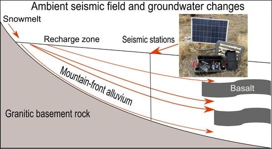
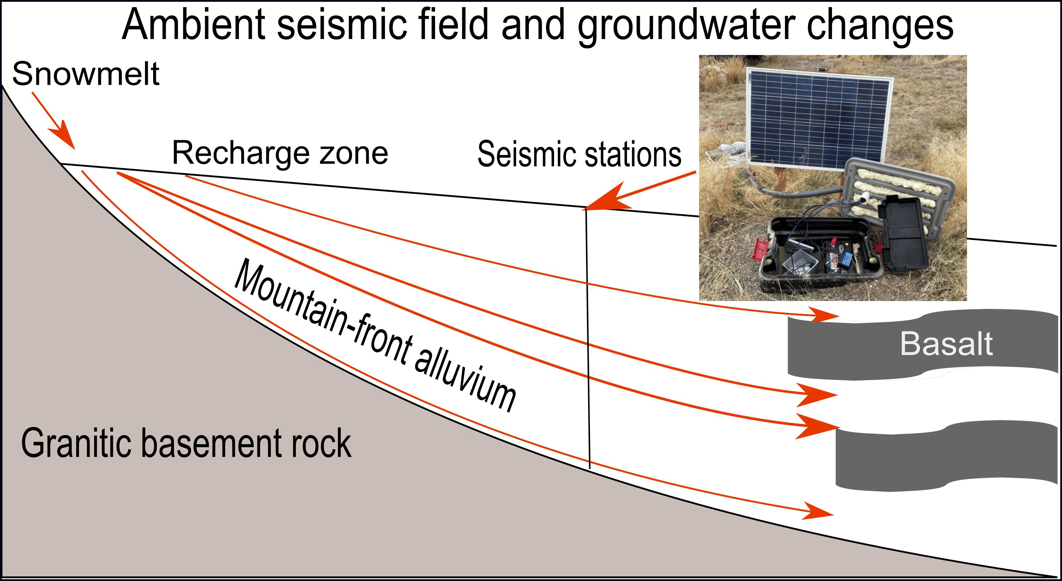
1.1. Recharge Zone
1.2. Passive Seismic Monitoring for Estimating Groundwater Levels
2. Materials and Methods
2.1. Seismometer and Station Construction
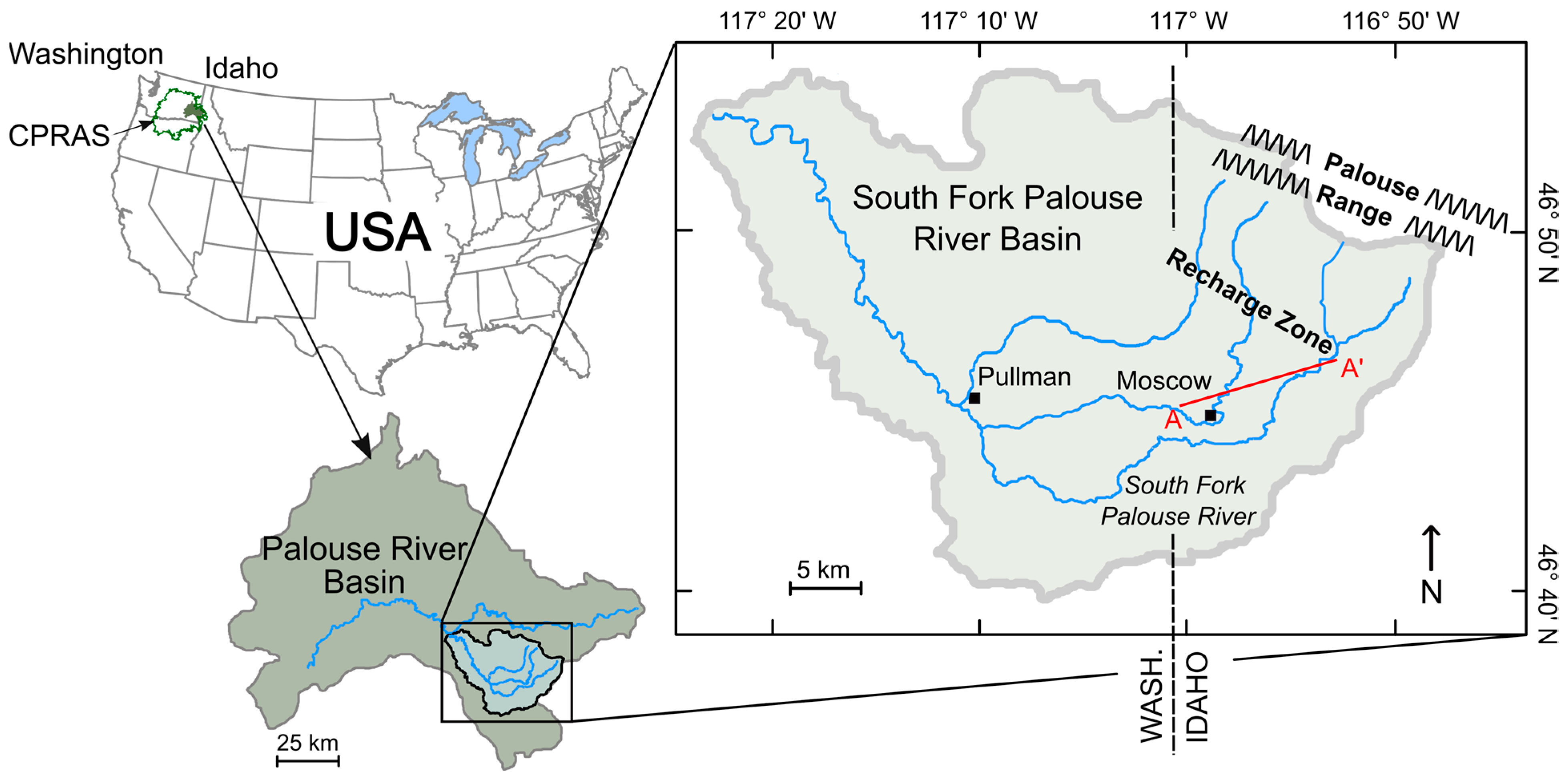
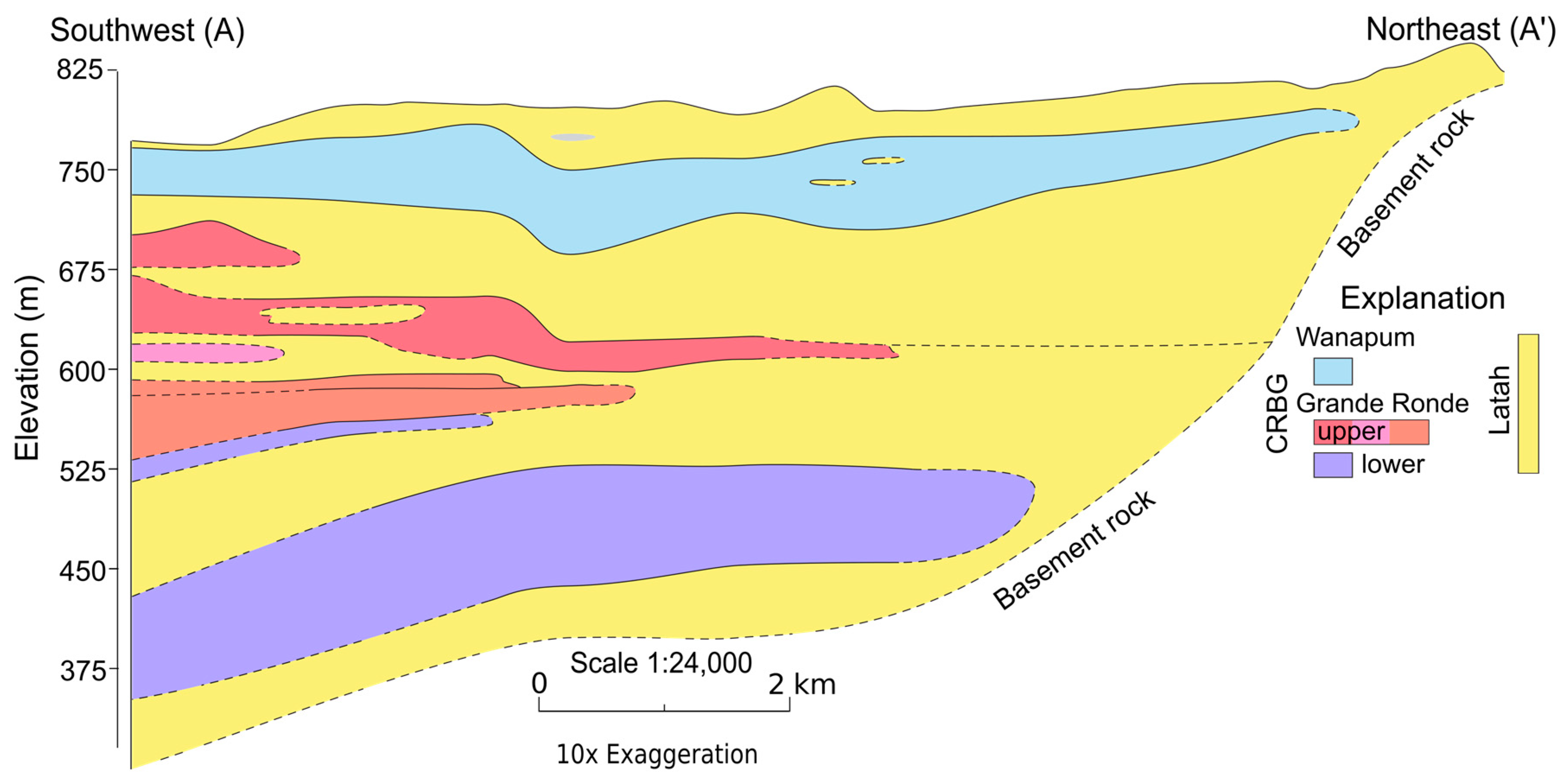
2.2. Seismic Station Locations
2.3. Seismic Station Network and Quantifying Recharge

2.4. Identifying Applicable Waveforms in the Ambient Seismic Field
2.5. Velocity Changes to Groundwater Levels
2.6. Interpretations of Hydraulic Conductivity, Gradient, and Recharge
3. Results
3.1. Velocity Changes and Relation to Groundwater
3.2. Converting Seismic Velocity to Groundwater
3.3. Recharge Volumes by Network Segment
4. Discussion
5. Conclusions
Author Contributions
Funding
Data Availability Statement
Acknowledgments
Conflicts of Interest
References
- Candel, J.; Brooks, E.; Sánchez-Murillo, R.; Grader, G.; Dijksma, R. Identifying Groundwater Recharge Connections in the Moscow (USA) Sub-Basin Using Isotopic Tracers and a Soil Moisture Routing Model. Hydrogeol. J. 2016, 24, 1739–1751. [Google Scholar] [CrossRef]
- Custodio, E. Trends in Groundwater Pollution: Loss of Groundwater Quality & Related Services; Global Environment Facility and the Food and Agriculture Organization of the United Nations: Barcelona, Spain, 2014. [Google Scholar]
- Llamas, M.; Custodio, E. Intensive Use of Groundwater: Challenges and Opportunities; A.A. Balkema Publishers: Madrid, Spain, 2002. [Google Scholar]
- Gleeson, T.; Wada, Y.; Bierkens, M.F.P.; van Beek, L.P.H. Water Balance of Global Aquifers Revealed by Groundwater Footprint. Nature 2012, 488, 197–201. [Google Scholar] [CrossRef] [PubMed]
- Foxworthy, B.L.; Washburn, R.L. Ground Water in the Pullman Area, Whitman County, Washington; U.S. Geological Survey: Washington, DC, USA, 1963.
- Robischon, S. Annual Water Use Report 2016; Palouse Basin Aquifer Committee: Moscow, ID, USA, 2016. [Google Scholar]
- Burns, E.R.; Snyder, D.T.; Haynes, J.V.; Waibel, M.S. Groundwater Status and Trends for the Columbia Plateau Regional Aquifer System, Washington, Oregon, and Idaho; U.S. Geological Survey: Washington, DC, USA, 2012.
- Bush, J.H.; Pierce, J.L.; Potter, G.N. Bedrock Geologic Map of the Moscow East Quadrangle, Latah County, Idaho; Idaho Geological Survey: Moscow, ID, USA, 2010. [Google Scholar]
- Bush, J.H.; Dunlap, P.; Reidel, S.P.; Kobayashi, D. Geologic Cross Sections Across the Moscow-Pullman Basin, Idaho and Washington; Idaho Geological Survey: Moscow, ID, USA, 2018. [Google Scholar]
- Bush, J.H.; Dunlap, P.; Reidel, S.P. Miocene Evolution of the Moscow-Pullman Basin, Idaho and Washington; Idaho Geological Survey: Moscow, ID, USA, 2018. [Google Scholar]
- Reidel, S.P.; Tolan, T.L.; Hooper, P.R.; Beeson, M.H.; Fecht, K.R.; Bentley, R.D.; Anderson, J.L. The Grande Ronde Basalt, Columbia River Basalt Group; Stratigraphic Descriptions and Correlations in Washington, Oregon, and Idaho. In Volcanism and Tectonism in the Columbia River Flood-Basalt Province; Geological Society of America: McLean, VA, USA, 1989; Volume 239, pp. 21–54. [Google Scholar]
- Beall, A.; Fiedler, F.; Boll, J.; Cosens, B. Sustainable Water Resource Management and Participatory System Dynamics. Case Study: Developing the Palouse Basin Participatory Model. Sustainability 2011, 3, 720–742. [Google Scholar] [CrossRef]
- Dhungel, R.; Fiedler, F. Water Balance to Recharge Calculation: Implications for Watershed Management Using Systems Dynamics Approach. Hydrology 2016, 3, 13. [Google Scholar] [CrossRef]
- Behrens, D.; Langman, J.B.; Brooks, E.S.; Boll, J.; Waynant, K.; Moberly, J.G.; Dodd, J.K.; Dodd, J.W. Tracing δ18O and δ2H in Source Waters and Recharge Pathways of a Fractured-Basalt and Interbedded-Sediment Aquifer, Columbia River Flood Basalt Province. Geosciences 2021, 11, 400. [Google Scholar] [CrossRef]
- Hernandez, H.P. Observations of Recharge to the Wanapum Aquifer System in the Moscow Area, Latah County, Idaho. Master’s Thesis, University of Idaho, Moscow, ID, USA, 2007. [Google Scholar]
- Kopp, W.P. Hydrogeology of the Upper Aquifer of the Pullman-Moscow Basin at the University of Idaho Aquaculture Site. Ph.D. Thesis, University of Idaho, Moscow, ID, USA, 1994. [Google Scholar]
- Leek, F. Hydrogeological Characterization of the Palouse Basin Basalt Aquifer System, Washington and Idaho. Master’s Thesis, Washington State University, Pullman, WA, USA, 2006. [Google Scholar]
- Tong, L. Hydrogeologic Characterization of a Multiple Aquifer Fractured Basalt System. Ph.D. Thesis, University of Idaho, Moscow, ID, USA, 1991. [Google Scholar]
- Lum II, W.E.; Smoot, J.L.; Ralston, D.R. Geohydrology and Numerical Model Analysis of Ground-Water Flow in the Pullman-Moscow Area, Washington and Idaho; US Geological Survey: Washington, DC, USA, 1990; p. 79.
- Medici, G.; Engdahl, N.B.; Langman, J.B. A Basin-Scale Groundwater Flow Model of the Columbia Plateau Regional Aquifer System in the Palouse (USA): Insights for Aquifer Vulnerability Assessment. Int. J. Environ. Res. 2021, 15, 299–312. [Google Scholar] [CrossRef]
- Medici, G.; Langman, J.B. Pathways and Estimate of Aquifer Recharge in a Flood Basalt Terrain; A Review from the South Fork Palouse River Basin (Columbia River Plateau, USA). Sustainability 2022, 14, 11349. [Google Scholar] [CrossRef]
- Ryu, J.H.; Contor, B.; Johnson, G.; Allen, R.; Tracy, J. System Dynamics to Sustainable Water Resources Management in the Eastern Snake Plain Aquifer Under Water Supply Uncertainty1: System Dynamics to Sustainable Water Resources Management in the Eastern Snake Plain Aquifer Under Water Supply Uncertainty. J. Am. Water Resour. Assoc. 2012, 48, 1204–1220. [Google Scholar] [CrossRef]
- Provant, A.P. Geology and Hydrogeology of the Viola and Moscow West Quadrangles, Latah County, Idaho and Whitman County, Washington. Master’s Thesis, University of Idaho, Moscow, ID, USA, 1995. [Google Scholar]
- Bush, J.H.; Dunlap, P. Geologic Interpretations of Wells and Important Rock Outcrops in the Moscow-Pullman Basin and Vicinity, Idaho and Washington; Idaho Geological Survey: Moscow, ID, USA, 2018. [Google Scholar]
- Duckett, K.A.; Langman, J.B.; Bush, J.H.; Brooks, E.S.; Dunlap, P.; Welker, J.M. Isotopic Discrimination of Aquifer Recharge Sources, Subsystem Connectivity and Flow Patterns in the South Fork Palouse River Basin, Idaho and Washington, USA. Hydrology 2019, 6, 15. [Google Scholar] [CrossRef]
- Ackerman, D.J. Transmissivity of the Snake River Plain Aquifer at the Idaho National Engineering Laboratory, Idaho; U.S. Geological Survey: Washington, DC, USA, 1991.
- Duckett, K.A.; Langman, J.B.; Bush, J.H.; Brooks, E.S.; Dunlap, P.; Stanley, J.R. Noble Gases, Dead Carbon, and Reinterpretation of Groundwater Ages and Travel Time in Local Aquifers of the Columbia River Basalt Group. J. Hydrol. Amst. 2020, 581, 124400. [Google Scholar] [CrossRef]
- Langman, J.B.; Martin, J.; Gaddy, E.; Boll, J.; Behrens, D. Snowpack Aging, Water Isotope Evolution, and Runoff Isotope Signals, Palouse Range, Idaho, USA. Hydrology 2022, 9, 94. [Google Scholar] [CrossRef]
- Bush, J.H.; Dunlap, P.; Kodayashi, D. A Collection of Geologic Maps, Cross Sections, and Schematic Diagrams That Illustrate the Subsurface Geology of the Moscow-Pullman Basin and Vicinity; Palouse Basin Aquifer Committee: Moscow, ID, USA, 2019. [Google Scholar]
- Bohnhoff, M.; Dresen, G.; Ellsworth, W.L.; Ito, H. Passive Seismic Monitoring of Natural and Induced Earthquakes: Case Studies, Future Directions and Socio-Economic Relevance. In New Frontiers in Integrated Solid Earth Sciences; Cloetingh, S., Negendank, J., Eds.; International Year of Planet Earth; Springer: Dordrecht, The Netherlands, 2010; pp. 261–285. ISBN 978-90-481-2737-5. [Google Scholar]
- Mordret, A.; Courbis, R.; Brenguier, F.; Chmiel, M.; Garambois, S.; Mao, S.; Boué, P.; Campman, X.; Lecocq, T.; Van der Veen, W.; et al. Noise-Based Ballistic Wave Passive Seismic Monitoring—Part 2: Surface Waves. Geophys. J. Int. 2020, 221, 692–705. [Google Scholar] [CrossRef]
- Meier, U.; Shapiro, N.M.; Brenguier, F. Detecting Seasonal Variations in Seismic Velocities within Los Angeles Basin from Correlations of Ambient Seismic Noise. Geophys. J. Int. 2010, 181, 985–996. [Google Scholar] [CrossRef]
- Campillo, M.; Roux, P. Crust and Lithospheric Structure—Seismic Imaging and Monitoring with Ambient Noise Correlations. In Treatise on Geophysics; 2015; pp. 391–417. ISBN 978-0-444-53803-1. [Google Scholar]
- McNamara, D.E.; Boaz, R.I. Visualization of the Seismic Ambient Noise Spectrum. In Seisimic Ambient Noise; Nakata, N., Gualtieri, L., Fichtner, A., Eds.; Cambridge University Press: Cambridge, UK, 2019; ISBN 978-1-108-41708-2. [Google Scholar]
- Grêt, A.; Snieder, R.; Scales, J. Time-Lapse Monitoring of Rock Properties with Coda Wave Interferometry. J. Geophys. Res. Solid Earth 2006, 111. [Google Scholar] [CrossRef]
- Christensen, N.I.; Wang, H.F. The Influence of Pore Pressure and Confining Pressure on Dynamic Elastic Properties of Berea Sandstone. Geophysics 1985, 50, 207–213. [Google Scholar] [CrossRef]
- Clements, T.; Denolle, M.A. Tracking Groundwater Levels Using the Ambient Seismic Field. Geophys. Res. Lett. 2018, 45, 6459–6465. [Google Scholar] [CrossRef]
- Grêt, A.; Snieder, R.; Aster, R.C.; Kyle, P.R. Monitoring Rapid Temporal Change in a Volcano with Coda Wave Interferometry. Geophys. Res. Lett. 2005, 32. [Google Scholar] [CrossRef]
- Christensen, N.I. The Influence of Pore Pressure on Oceanic Crustal Seismic Velocities. J. Geodyn. 1986, 5, 45–48. [Google Scholar] [CrossRef]
- Lecocq, T.; Longuevergne, L.; Pedersen, H.A.; Brenguier, F.; Stammler, K. Monitoring Ground Water Storage at Mesoscale Using Seismic Noise: 30 Years of Continuous Observation and Thermo-Elastic and Hydrological Modeling. Sci. Rep. 2017, 7, 14241. [Google Scholar] [CrossRef]
- Shapiro, N.M.; Campillo, M. Emergence of Broadband Rayleigh Waves from Correlations of the Ambient Seismic Noise. Geophys. Res. Lett. 2004, 31. [Google Scholar] [CrossRef]
- Wang, Q.-Y.; Brenguier, F.; Campillo, M.; Lecointre, A.; Takeda, T.; Aoki, Y. Seasonal Crustal Seismic Velocity Changes Throughout Japan. J. Geophys. Res. Solid Earth 2017, 122, 7987–8002. [Google Scholar] [CrossRef]
- Gassenmeier, M.; Sens-Schönfelder, C.; Delatre, M.; Korn, M. Monitoring of Environmental Influences on Seismic Velocity at the Geological Storage Site for CO2 in Ketzin (Germany) with Ambient Seismic Noise. Geophys. J. Int. 2015, 200, 524–533. [Google Scholar] [CrossRef]
- Tsai, V.C. Understanding the Amplitudes of Noise Correlation Measurements. J. Geophys. Res. Solid Earth 2011, 116. [Google Scholar] [CrossRef]
- Voisin, C.; Guzmán, M.A.R.; Réfloch, A.; Taruselli, M.; Garambois, S. Groundwater Monitoring with Passive Seismic Interferometry. J. Water Resour. Prot. 2017, 9, 1414–1427. [Google Scholar] [CrossRef]
- Garambois, S.; Voisin, C.; Romero Guzman, M.A.; Brito, D.; Guillier, B.; Réfloch, A. Analysis of Ballistic Waves in Seismic Noise Monitoring of Water Table Variations in a Water Field Site: Added Value from Numerical Modelling to Data Understanding. Geophys. J. Int. 2019, 219, 1636–1647. [Google Scholar] [CrossRef]
- Prieto, G.A.; Denolle, M.; Lawrence, J.F.; Beroza, G.C. On Amplitude Information Carried by the Ambient Seismic Field. Comptes Rendus Geosci. 2011, 343, 600–614. [Google Scholar] [CrossRef]
- Berryman, J.G. Seismic Wave Attenuation in Fluid-Saturated Porous Media. In Scattering and Attenuations of Seismic Waves, Part I; Aki, K., Wu, R.-S., Eds.; Pageoph Topical Volumes; Birkhäuser: Basel, Switzerland, 1988; pp. 423–432. ISBN 978-3-0348-7722-0. [Google Scholar]
- Nakata, N.; Gualtieri, L.; Fichtner, A. Seisimic Ambient Noise; Nakata, N., Gualtieri, L., Fichtner, A., Eds.; Cambridge University Press: Cambridge, UK, 2019; ISBN 978-1-108-41708-2. [Google Scholar]
- Krischer, L.; Megies, T.; Barsch, R.; Beyreuther, M.; Lecocq, T.; Caudron, C.; Wassermann, J. ObsPy: A Bridge for Seismology into the Scientific Python Ecosystem. Comput. Sci. Discov. 2015, 8, 014003. [Google Scholar] [CrossRef]
- McNamara, D.E.; Buland, R.P. Ambient Noise Levels in the Continental United States. Bull. Seismol. Soc. Am. 2004, 94, 1517–1527. [Google Scholar] [CrossRef]
- Lecocq, T.; Caudron, C.; Brenguier, F. MSNoise, A Python Package for Monitoring Seismic Velocity Changes Using Ambient Seismic Noise. Seismol. Res. Lett. 2014, 85, 715–726. [Google Scholar] [CrossRef]
- Sajid, M.; Ghosh, D. A Fast and Simple Method of Spectral Enhancement. Geophysics 2014, 79, V75–V80. [Google Scholar] [CrossRef]
- Schimmel, M.; Stutzmann, E.; Ventosa, S. Low-Frequency Ambient Noise Autocorrelations: Waveforms and Normal Modes. Seismol. Res. Lett. 2018, 89, 1488–1496. [Google Scholar] [CrossRef]
- Clarke, D.; Zaccarelli, L.; Shapiro, N.M.; Brenguier, F. Assessment of Resolution and Accuracy of the Moving Window Cross Spectral Technique for Monitoring Crustal Temporal Variations Using Ambient Seismic Noise. Geophys. J. Int. 2011, 186, 867–882. [Google Scholar] [CrossRef]
- Sánchez-Sesma, F.J.; Campillo, M. Retrieval of the Green’s Function from Cross Correlation: The Canonical Elastic Problem. Bull. Seismol. Soc. Am. 2006, 96, 1182–1191. [Google Scholar] [CrossRef]
- Nanda, N.C. Seismic Wave and Rock-Fluid Properties. In Seismic Data Interpretation and Evaluation for Hydrocarbon Exploration and Production: A Practitioner’s Guide; Nanda, N.C., Ed.; Advances in Oil and Gas Exploration & Production; Springer International Publishing: Cham, Switzerland, 2021; pp. 3–23. ISBN 978-3-030-75301-6. [Google Scholar]
- National Water and Climate Center, NWCC Report Generator—Idaho SNOTEL Moscow Mountain Site, Average Precipitation Accumulation (1981–2010). Available online: https://wcc.sc.egov.usda.gov/reportGenerator/view/customGroupByMonthReport/daily/989:id:SNTL|id=%22%22|name/1980-10-01,1981-09-30/PREC::average_1981 (accessed on 9 January 2019).
- Sánchez-Murillo, R.; Brooks, E.S.; Elliot, W.J.; Boll, J. Isotope Hydrology and Baseflow Geochemistry in Natural and Human-Altered Watersheds in the Inland Pacific Northwest, USA. Isotopes Environ. Health Stud. 2015, 51, 231–254. [Google Scholar] [CrossRef]
- Bush, J.H. Bedrock Geologic Map of the Viola Quadrangle, Latah County, Idaho, and Whitman County, Washington; Idaho Geological Survey: Moscow, ID, USA, 1998. [Google Scholar]
- Pierce, J.L. Geology and Hydrology of the Moscow East and Robinson Lake Quadrangles, Latah County, Idaho. Master’s Thesis, University of Idaho, Moscow, ID, USA, 1998. [Google Scholar]
- Domenico, P.A.; Schwartz, F.W. Physical and Chemical Hydrogeology, 2nd ed.; Wiley & Sons: New York, NY, USA, 1997; ISBN 978-0-471-59762-9. [Google Scholar]
- Freeze, R.A.; Cherry, J.A. Groundwater; Prentice-Hall: Englewood Cliffs, NJ, USA, 1979; ISBN 978-0-13-365312-0. [Google Scholar]


| Station ID | Latitude 1 | Longitude 1 | Elevation (m) 2 |
|---|---|---|---|
| 1 | 46.78935 | −117.010 | 848 |
| 2 | 46.78417 | −116.987 | 853 |
| 3 | 46.77367 | −116.975 | 824 |
| 4 | 46.77975 | −116.972 | 848 |
| 5 | 46.77078 | −116.951 | 846 |
| 6 | 46.76875 | −116.936 | 863 |
| Station pairs | 1–2 | 2–3 | 2–4 | 3–5 | 4–5 | 5–6 |
| Recharge segments | A | B 1 | C 1 | D 1 | E 1 | F |
| Period | Date Range (2020–2021) | ΔGWL (m) | Δdv/v (%) | Cperiod |
|---|---|---|---|---|
| 1 | October | +2.19 | −0.07 | 31.2 |
| 2 | November–May | +0.93 | −0.20 | 4.6 |
| 3 | June | −1.89 | +0.05 | 37.3 |
| 4 | July–September | −0.62 | +0.12 | 5.3 |
| Network Segment | Hydraulic Conductivity (m/d) | Saturated Thickness (m) | Station Distance (m) | Hydraulic Gradient | Potential Recharge (m3/d) | Adjusted Recharge 1 (m3/d) |
|---|---|---|---|---|---|---|
| A | 0.024 | 8.0 | 1812 | 0.030 | 10.3 | 10.3 |
| B 1 | 0.033 | 17.8 | 1253 | 0.031 | 22.4 | 43.0 |
| C 1 | 0.033 | 23.5 | 1500 | 0.055 | 63.5 | |
| D 1 | 0.042 | 32.9 | 1883 | 0.080 | 210.6 | 189.8 |
| E 1 | 0.042 | 47.6 | 1927 | 0.044 | 169.0 | |
| F | 0.052 | 44.9 | 1130 | 0.063 | 164.6 | 164.6 |
| Network sum (m3/d): | 407.7 | |||||
Disclaimer/Publisher’s Note: The statements, opinions and data contained in all publications are solely those of the individual author(s) and contributor(s) and not of MDPI and/or the editor(s). MDPI and/or the editor(s) disclaim responsibility for any injury to people or property resulting from any ideas, methods, instructions or products referred to in the content. |
© 2022 by the authors. Licensee MDPI, Basel, Switzerland. This article is an open access article distributed under the terms and conditions of the Creative Commons Attribution (CC BY) license (https://creativecommons.org/licenses/by/4.0/).
Share and Cite
Buzzard, Q.; Langman, J.B.; Behrens, D.; Moberly, J.G. Monitoring the Ambient Seismic Field to Track Groundwater at a Mountain–Front Recharge Zone. Geosciences 2023, 13, 9. https://doi.org/10.3390/geosciences13010009
Buzzard Q, Langman JB, Behrens D, Moberly JG. Monitoring the Ambient Seismic Field to Track Groundwater at a Mountain–Front Recharge Zone. Geosciences. 2023; 13(1):9. https://doi.org/10.3390/geosciences13010009
Chicago/Turabian StyleBuzzard, Quinn, Jeff B. Langman, David Behrens, and James G. Moberly. 2023. "Monitoring the Ambient Seismic Field to Track Groundwater at a Mountain–Front Recharge Zone" Geosciences 13, no. 1: 9. https://doi.org/10.3390/geosciences13010009
APA StyleBuzzard, Q., Langman, J. B., Behrens, D., & Moberly, J. G. (2023). Monitoring the Ambient Seismic Field to Track Groundwater at a Mountain–Front Recharge Zone. Geosciences, 13(1), 9. https://doi.org/10.3390/geosciences13010009