

The GOGIRA System: An Innovative Method for Landslides Digital Mapping


Abstract
:
1. Introduction
2. Materials and Methods
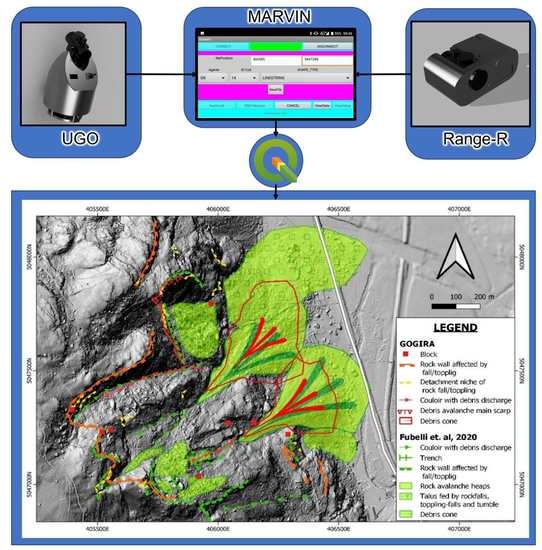
2.1. GOGIRA as GIS System
- CoordFinder, an algorithm to convert local spherical coordinates into a cartographic reference system;
- Two devices, UGO (User-based Geomorphic Observer) and Range-R (Remote Rangefinder), designed for target local spherical coordinates acquisition;
- MARVIN, a smartphone Android application developed to collect UGO and Range-R data, set information about morphogenetic processes, and type of morphometry;
- A semi-automatic cartographic import and legend procedure for QGIS projects.
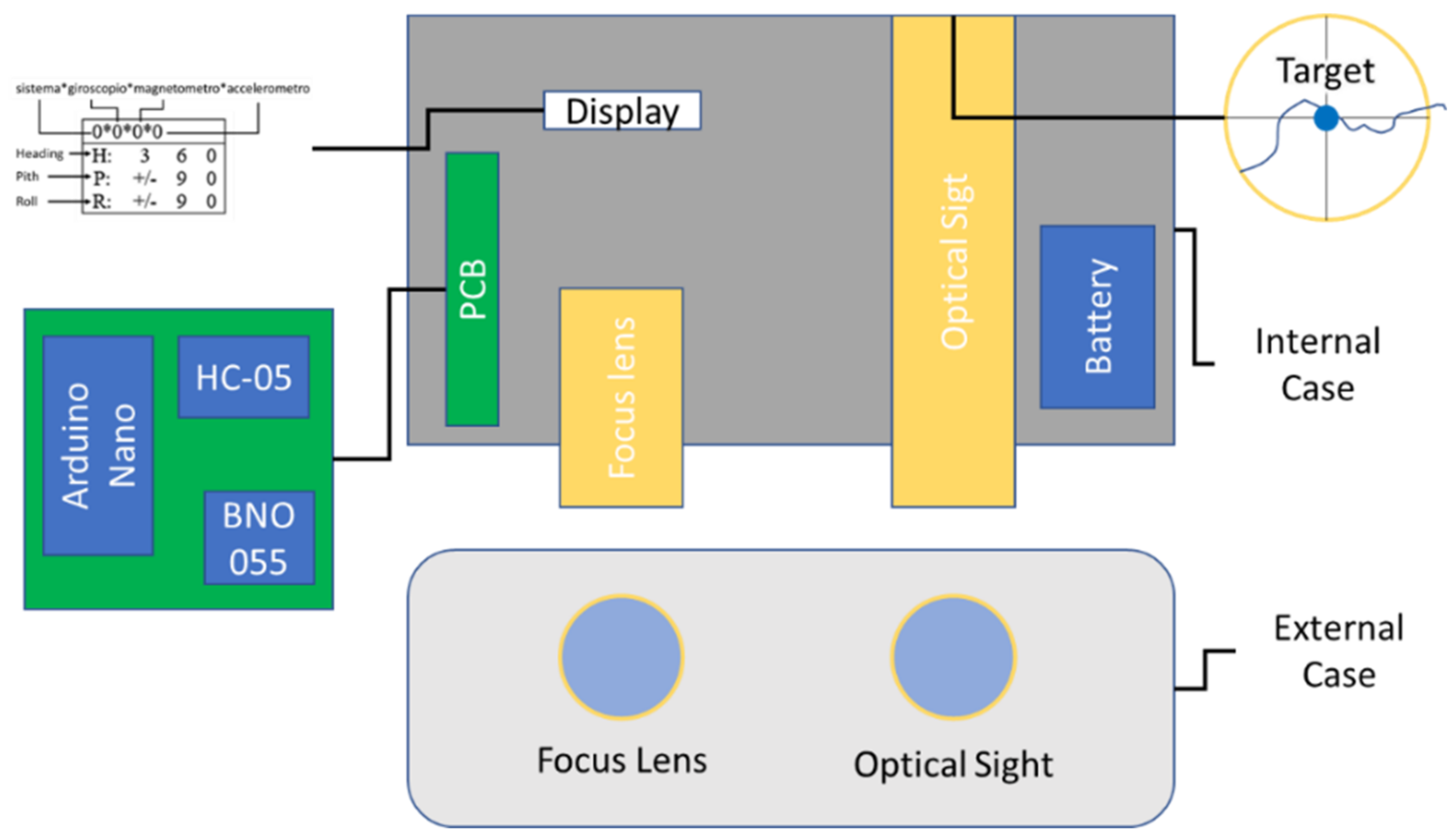
2.2. Prototypes
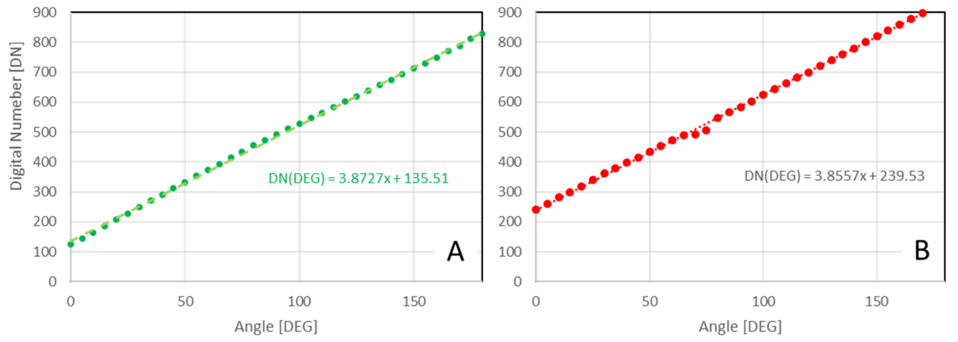
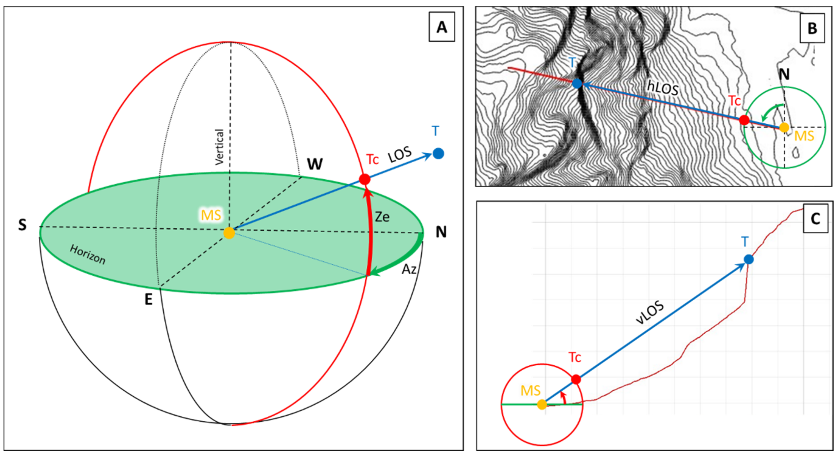
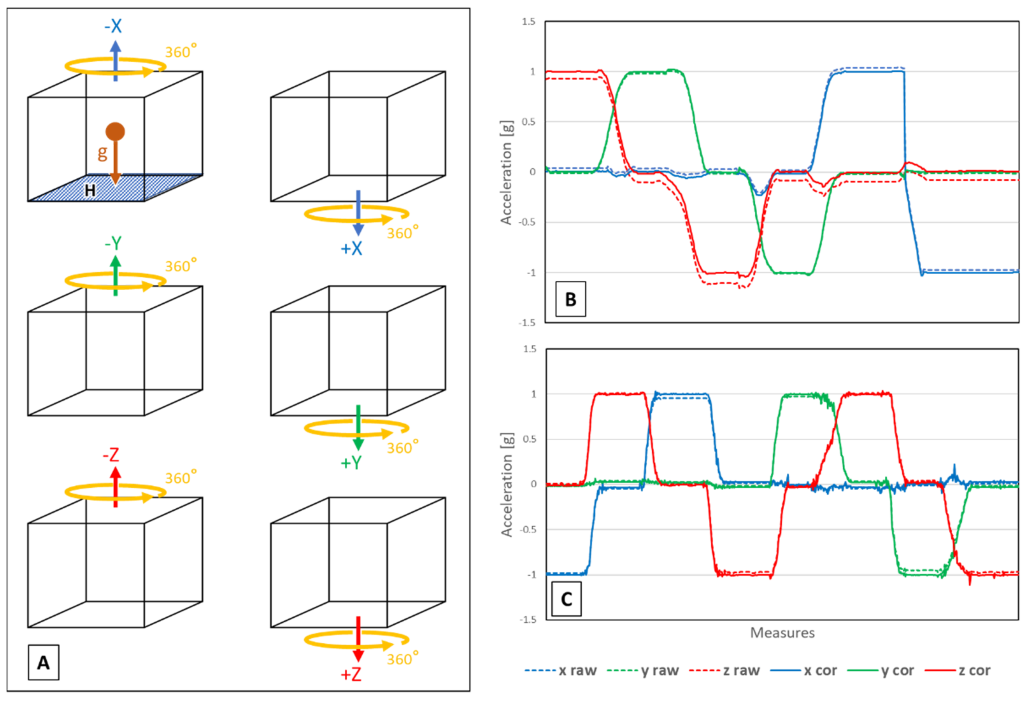
2.2.1. CoordFinder Algorithm
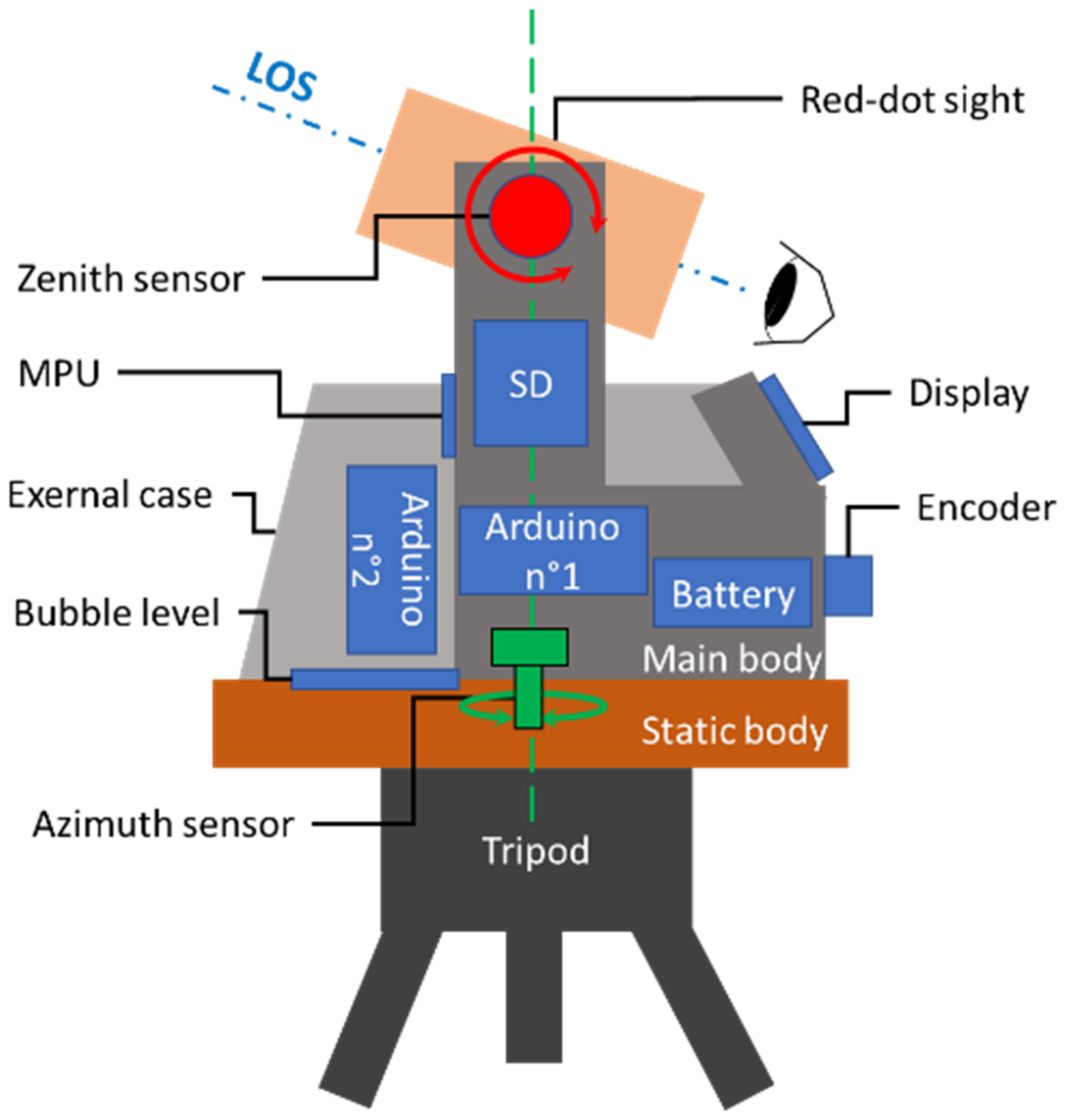
2.2.2. Tools
- n° 2 Rotary potentiometer;
- n° 1 Rotary encoder;
- n° 1 HC-05 Bluetooth module;
- n° 2 Arduino Nano microcontroller;
- n° 1 MPU6050 Inertial Motion Unit (IMU);
- n° 1 SSD1306 OLED display;
- n° 1 SD-card module;
- n° 1 Toroidal bubble-level;
- n° 1 9-volt battery cell;
- n° 1 Red-dot optical sight;
- n° 1 Tripod.
- n° 1 Arduino Nano microcontroller;
- n° 1 BNO055 Attitude and Heading Reference System (AHRS)
- n° 1 SSD1306 OLED display;
- n° 1 HC-05 Bluetooth module;
- n° 1 optical sight 10x zoom;
- n° 1 9-volt battery cell.
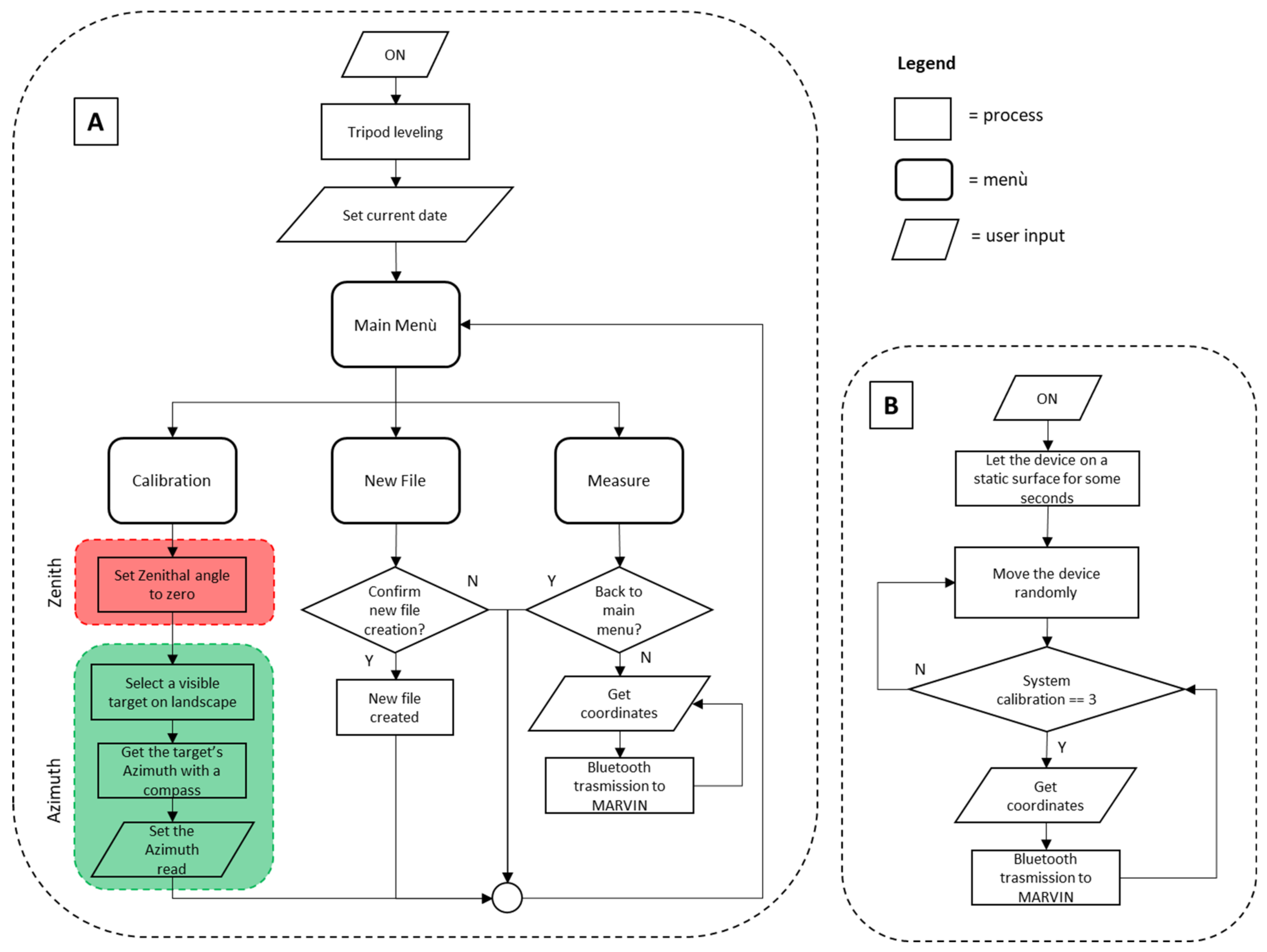
2.3. Procedures and Data
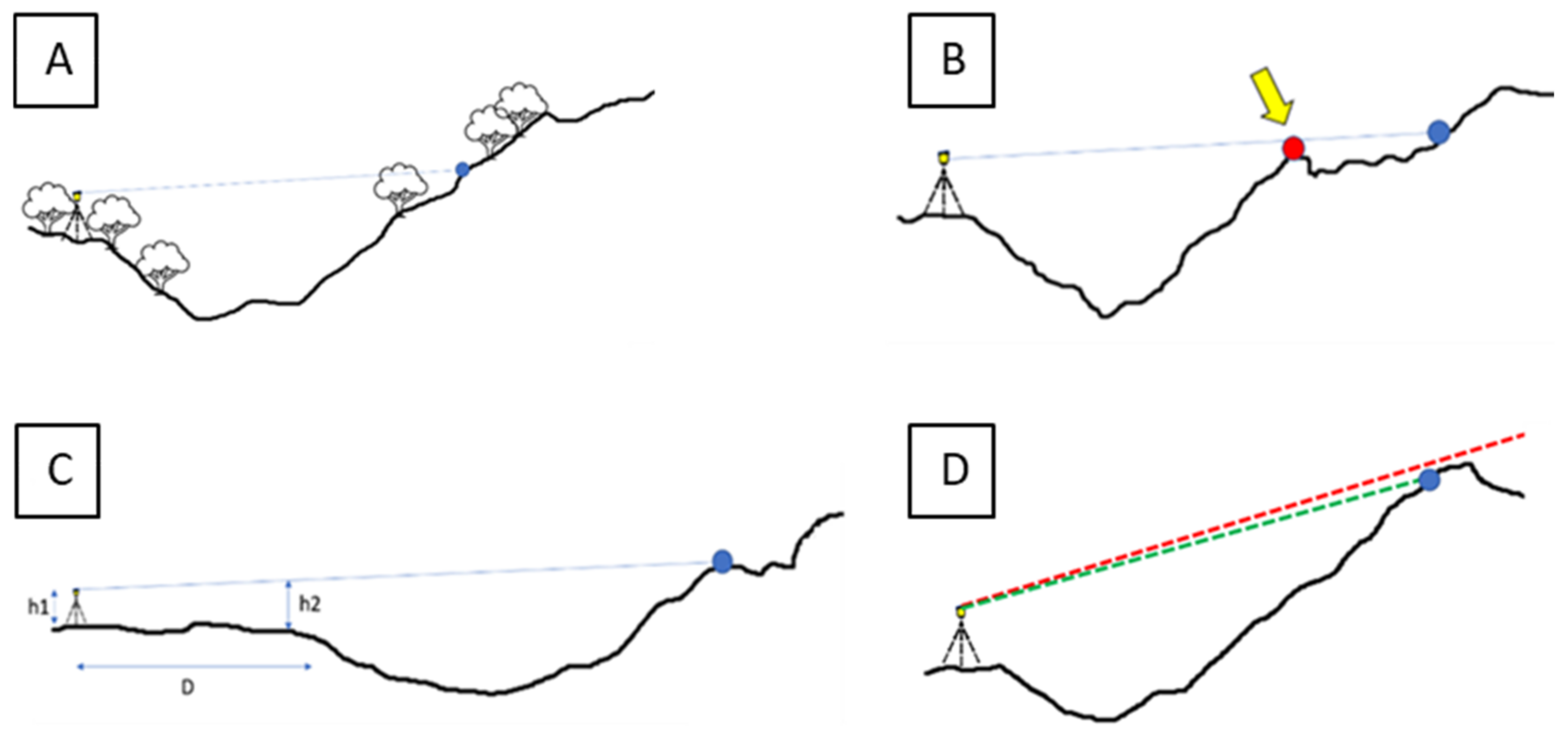
2.3.1. Field Survey
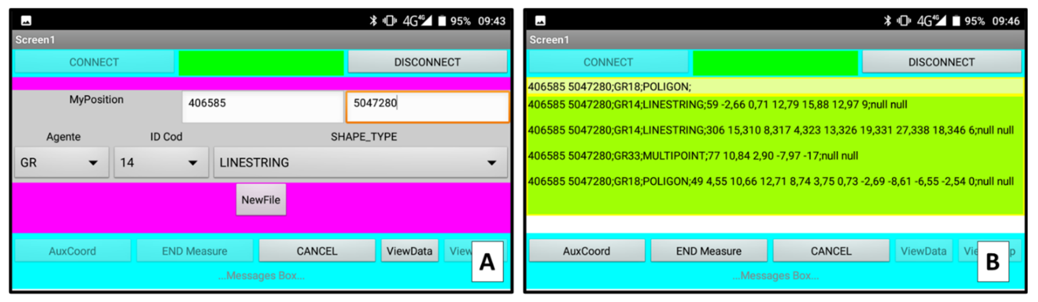
2.3.2. MARVIN
2.3.3. CoordFinder
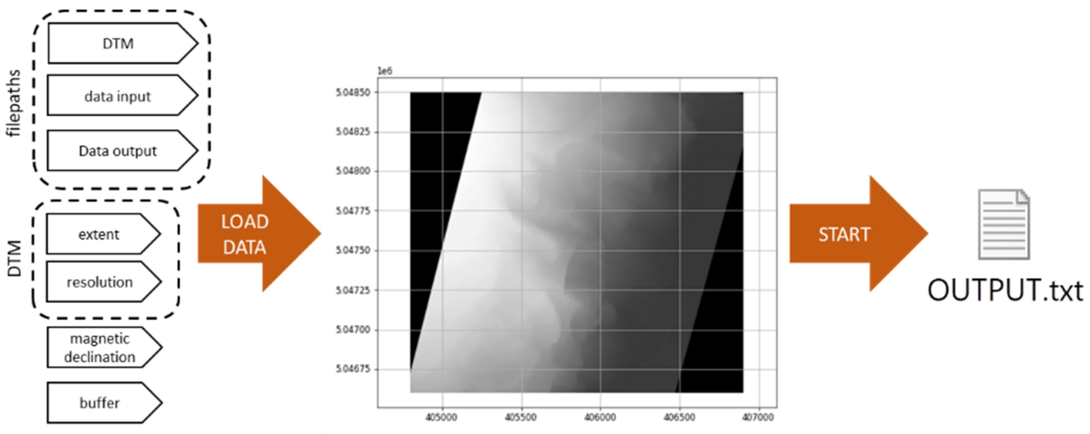
2.3.4. QGIS Data Import
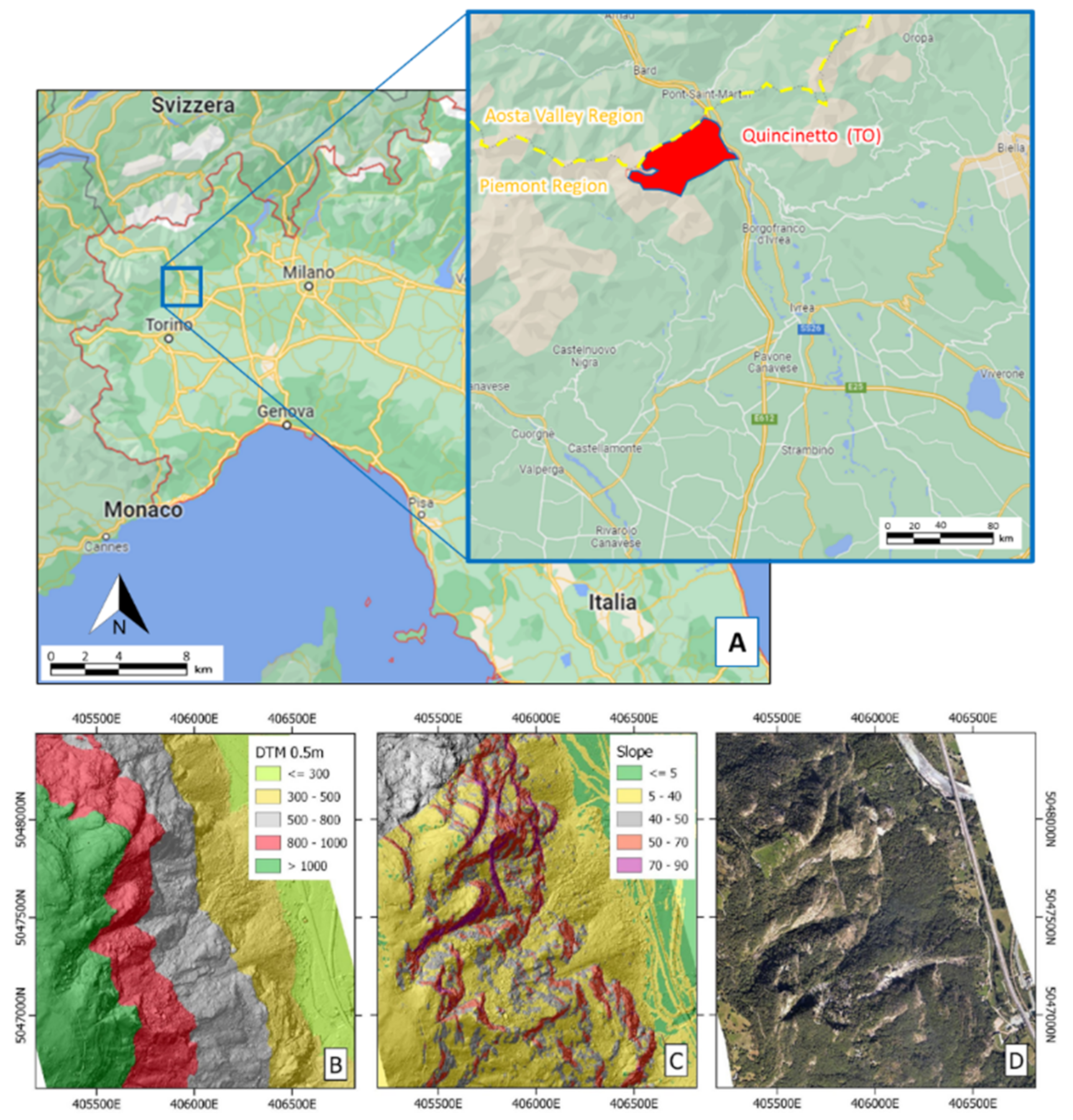
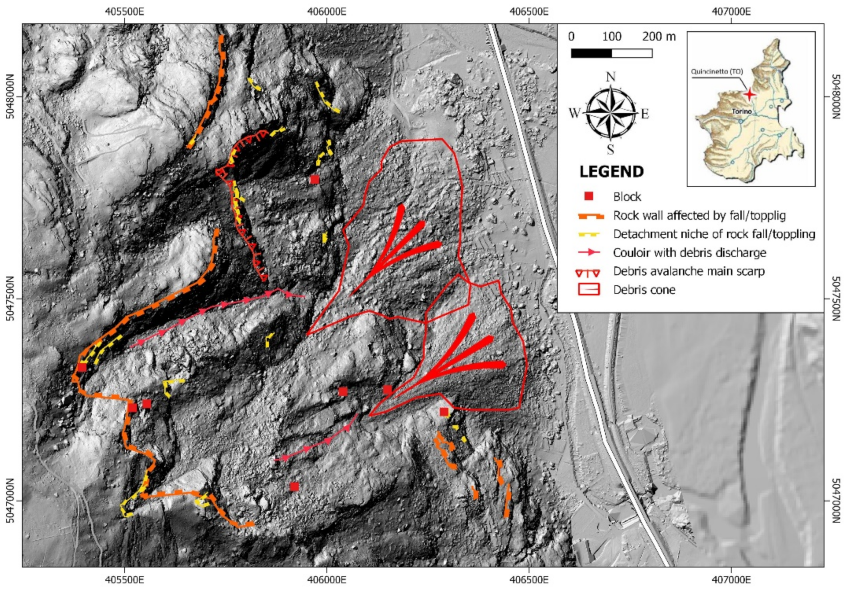
2.4. Field Test: Quincinetto Landslide System
- Estimate the mapping precision with varying distance from the measuring station and targets (metric difference);
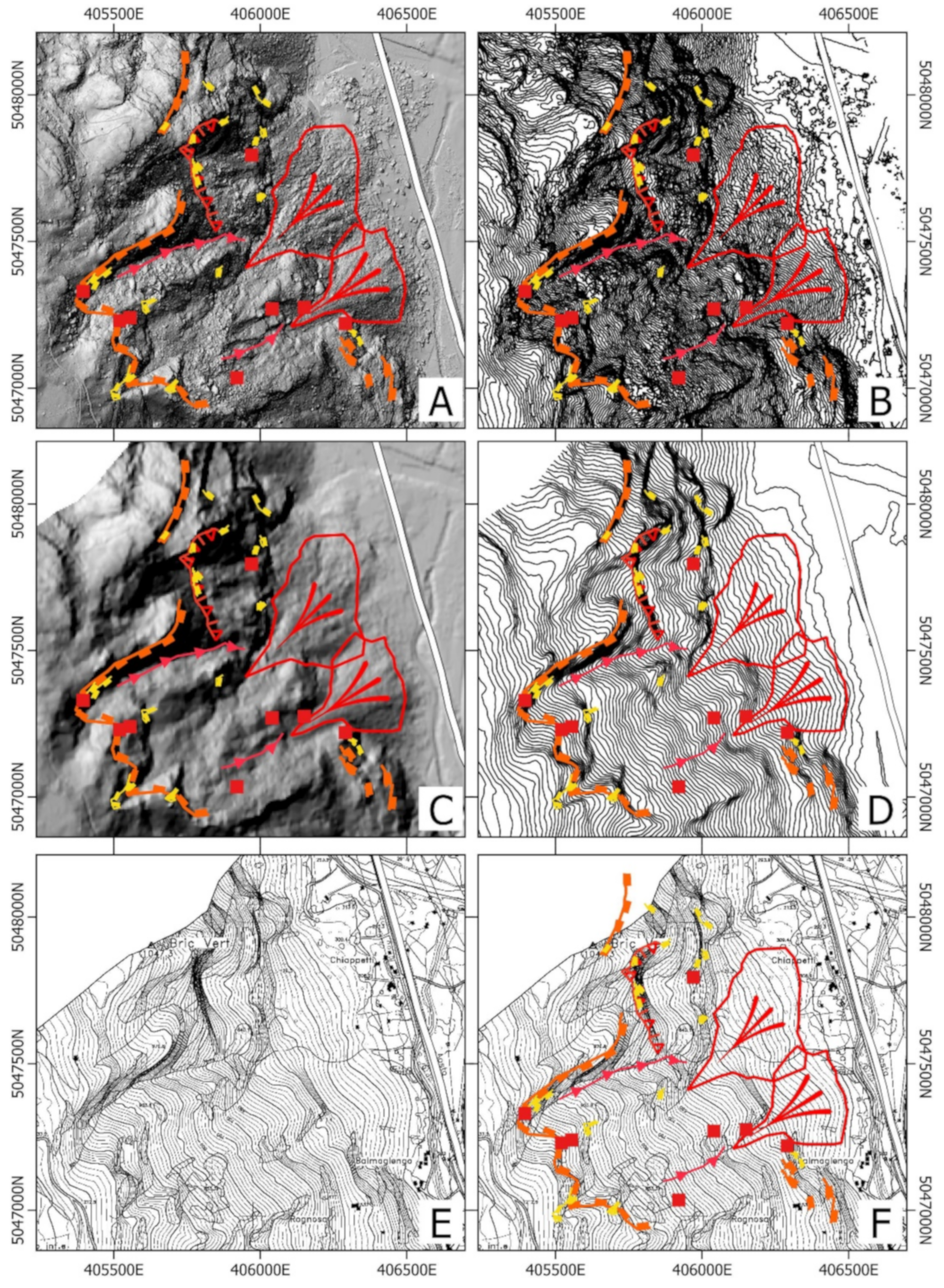
- Check the morphometric coherence between the mapped shapes and the land morphometry (graphical comparison);
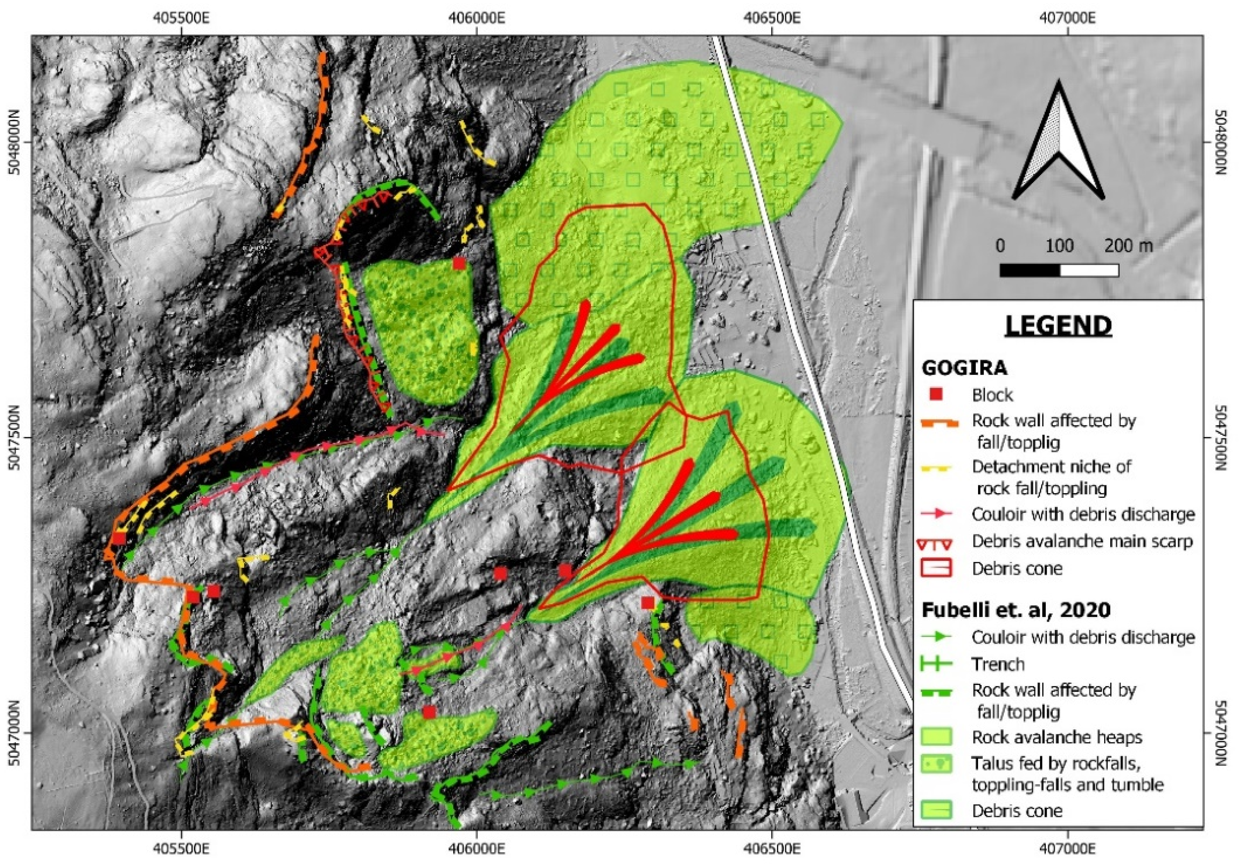
- Evaluate GOGIRA’s final mapping result by comparison with a highly detailed geomorphological map made with modern tested methods (maps comparison).
3. Application and Results
3.1. Data Acquisition and Elaboration
3.2. Metric Difference
3.3. Graphical Comparison
3.4. Maps Comparison
4. Discussion
5. Conclusions
- DNC can improve and optimize geomorphological mapping;
- A GIS-structured project can be used to developed new methods for DNC with standardized and interconnected devices and software;
- GOGIRA proved to be a valid system for geomorphological DNC applied to a complex landslide system. Considering the early stage of development, results were excellent for mapping linear and point objects, as for polygonal elements, more studies must be conducted to improve accuracy and precision;
- Finally, for both INC and DNC, high-resolution DTMs are fundamental for a good quality, detailed geomorphological map, while CTR is often not suitable for mapping meso or micro-scale elements.
Author Contributions
Funding
Data Availability Statement
Acknowledgments
Conflicts of Interest
References
- Passarge, S. Erla¨uterungen Zu Lief. 1, Morphologie Des Messtischblattes Stadtremba (1:25,000). Mitt. Geogr. Gesell. 1914, 28. [Google Scholar]
- Smith, M.J.; Paron, P.; Griffiths, J.S. Geomorphological Mapping: Methods and Applications. In Developments in Earth Surface Processes, 1st ed.; Elsevier: Amsterdam, The Netherlands; New York, NY, USA, 2011; ISBN 978-0-444-53446-0. [Google Scholar]
- van Zuidam, R.A.; van Zuidam-Cancelado, F.I. Terrain Analysis and Classification Using Aerial Photographs; International Institute for Aerial Survey and Earth Sciences: Enschede, The Netherlands, 1979; Volume 7, ISBN 978-90-6164-038-7. [Google Scholar]
- Ershad, A. Geographic Information System (GIS): Definition, Development, Applications & Components. Jalpaiguri. 2020. Available online: https://www.researchgate.net/publication/340182760_Geographic_Information_System_GIS_Definition_Development_Applications_Components (accessed on 6 May 2022).
- Yue, P.; Tan, Z. GIS Databases and NoSQL Databases. In Comprehensive Geographic Information Systems; Elsevier: Amsterdam, The Netherlands, 2018; pp. 50–79. ISBN 978-0-12-804793-4. [Google Scholar]
- Gandhi, V.; Kang, J.M.; Shekhar, S. Spatial Databases. In Wiley Encyclopedia of Computer Science and Engineering; Wah, B.W., Ed.; John Wiley & Sons, Inc.: Hoboken, NJ, USA, 2008; ISBN 978-0-470-05011-8. [Google Scholar]
- Cartografia Numerica: Manuale Pratico per l’utilizzo Dei GIS, 1st ed.; Dainelli, N. (Ed.) Dario Flaccovio: Palermo, Italy, 2008; ISBN 978-88-7758-789-3. [Google Scholar]
- Kramer, J. Digital Mapping Systems for Field Data Collection. In Digital Mapping Techniques ’00-Workshop Proceedings; U.S. Geological Survey: Lexington, KY, USA, 2000; p. 210. [Google Scholar]
- Guzzetti, F.; Mondini, A.C.; Cardinali, M.; Fiorucci, F.; Santangelo, M.; Chang, K.-T. Landslide Inventory Maps: New Tools for an Old Problem. Earth-Sci. Rev. 2012, 112, 42–66. [Google Scholar] [CrossRef]
- van Asselen, S.; Seijmonsbergen, A.C. Expert-Driven Semi-Automated Geomorphological Mapping for a Mountainous Area Using a Laser DTM. Geomorphology 2006, 78, 309–320. [Google Scholar] [CrossRef]
- Ferrero, A.M.; Forlani, G.; Roncella, R.; Voyat, H.I. Advanced Geostructural Survey Methods Applied to Rock Mass Characterization. Rock Mech. Rock Eng. 2009, 42, 631–665. [Google Scholar] [CrossRef]
- Nikolakopoulos, K.G.; Kyriou, A.; Koukouvelas, I.K. Developing a Guideline of Unmanned Aerial Vehicle’s Acquisition Geometry for Landslide Mapping and Monitoring. Appl. Sci. 2022, 12, 4598. [Google Scholar] [CrossRef]
- Parrot, J.F.; Ramírez Núñez, C. Artefactos y Correcciones a Los Modelos Digitales de Terreno Provenientes Del Lídar. Investig. Geográficas 2016, 90, 28–39. [Google Scholar] [CrossRef]
- Mirik, M.; Chaudhuri, S.; Surber, B.; Ale, S.; James Ansley, R. Detection of Two Intermixed Invasive Woody Species Using Color Infrared Aerial Imagery and the Support Vector Machine Classifier. J. Appl. Remote. Sens. 2013, 7, 073588. [Google Scholar] [CrossRef]
- Perotti, L.; Lasagna, M.; Clemente, P.; Dino, G.A.; De Luca, D.A. Remote Sensing and Hydrogeological Methodologies for Irrigation Canal Water Losses Detection: The Naviglio Di Bra Test Site (NW-Italy). In Engineering Geology for Society and Territory-Volume 3; Lollino, G., Arattano, M., Rinaldi, M., Giustolisi, O., Marechal, J.-C., Grant, G.E., Eds.; Springer International Publishing: Cham, Switzerland, 2015; pp. 19–22. ISBN 978-3-319-09053-5. [Google Scholar]
- Solano Acosta, J.D.; Despaigne Diaz, A.I.; Pearse, J. Morphotectonic Analysis of the Upper Guajira, Colombia. A GIS and Remote Sensing Approach. Preprints 2020, 37, 2020100476. [Google Scholar] [CrossRef]
- ECOSTRESS Speclib. Available online: https://speclib.jpl.nasa.gov/library (accessed on 6 May 2022).
- Sousa, J.J.; Ruiz, A.M.; Hanssen, R.F.; Bastos, L.; Gil, A.J.; Galindo-Zaldívar, J.; Sanz de Galdeano, C. PS-InSAR Processing Methodologies in the Detection of Field Surface Deformation—Study of the Granada Basin (Central Betic Cordilleras, Southern Spain). J. Geodyn. 2010, 49, 181–189. [Google Scholar] [CrossRef]
- Fubelli, G. Rapporto tecnico: Indagini a Supporto della Fase A degli Interventi Finalizzati alla Rimozione delle Porzioni Rocciose Instabili dal Fenomeno Franoso a Monte della Frazione Chiappetti (Quincinetto, TO); Università degli Studi di Torino, Dipartimento di Scienze della Terra: Torino, Italy, 2020; p. 83. [Google Scholar]
- Clegg, P.; Bruciatelli, L.; Domingos, F.; Jones, R.R.; De Donatis, M.; Wilson, R.W. Digital Geological Mapping with Tablet PC and PDA: A Comparison. Comput. Geosci. 2006, 32, 1682–1698. [Google Scholar] [CrossRef]
- Cipriani, A.; Citton, P.; Romano, M.; Fabbi, S. Testing Two Open-Source Photogrammetry Software as a Tool to Digitally Preserve and Objectively Communicate Significant Geological Data: The Agolla Case Study (Umbria-Marche Apennines). IJG 2016, 135, 199–209. [Google Scholar] [CrossRef]
- Vosselman, G.; Gorte, B.G.H.; Sithole, G.; Rabbani, T.B. Recognising Structure in Laser Scanner Point Clouds. Inter. Arch. Photogramm. Remote Sens. Spatial Inf. Sci. 2003, 46, 33–38. [Google Scholar]
- Brown, K.; Sprinkel, D. Geologic Field Mapping Using a Rugged Tablet Computer. In Digital Mapping Techniques’ 07 Workshop Proceedings: US Geological Survey Open-File Report; US Geological Survey: Columbia, MO, USA, 2008; pp. 53–58. [Google Scholar]
- De Donatis, M.; Alberti, M.; Cipicchia, M.; Guerrero, N.M.; Pappafico, G.F.; Susini, S. Workflow of digital field mapping and drone-aided survey for the identification and characterization of capable faults: The case of a normal fault system in the monte nerone area (Northern Apennines, Italy). IJGI 2020, 9, 616. [Google Scholar] [CrossRef]
- Whitmeyer, S.J.; Pyle, E.J.; Pavlis, T.L.; Swanger, W.; Roberts, L. Modern approaches to field data collection and mapping: Digital methods, crowdsourcing, and the future of statistical analyses. J. Struct. Geol. 2019, 125, 29–40. [Google Scholar] [CrossRef]
- Friedrich, C. Comparison of ArcGIS and QGIS for Applications in Sustainable Spatial Planning. Master’s Thesis, University of Vienna, Wien, Austria, 2014. [Google Scholar]
- Universal Transvers Mercator. Available online: http://wiki.gis.com/wiki/index.php/Universal_Transverse_Mercator (accessed on 6 May 2022).
- Wold Geodetic System. 1984. Available online: http://wiki.gis.com/wiki/index.php/World_Geodetic_System#A_new_World_Geodetic_System:_WGS84 (accessed on 6 May 2022).
- Well-Known Text—GIS Wiki|The GIS Encyclopedia. Available online: http://wiki.gis.com/wiki/index.php/Well-known_text (accessed on 4 July 2022).
- Badea, A.C.; Badea, G. Considerations on Open Source GIS Software VS Proprietary GIS Software; Faculty of Geodesy, Surveying and Cadastre Department: Alba Iulia, Germany, 2018. [Google Scholar]
- Ruzza, G.; Guerriero, L.; Revellino, P.; Guadagno, F.M. A Multi-Module Fixed Inclinometer for Continuous Monitoring of Landslides: Design, Development, and Laboratory Testing. Sensors 2020, 20, 3318. [Google Scholar] [CrossRef] [PubMed]
- Rodríguez, B.G.; Meneses, J.S.; Garcia-Rodriguez, J. Implementation of a Low-Cost Rain Gauge with Arduino and Thingspeak. In Advances in Intelligent Systems and Computing, Processings of the 15th International Conference on Soft Computing Models in Industrial and Environmental Applications (SOCO 2020), Burgos, Spain, 6–18 September 2020; Herrero, Á., Cambra, C., Urda, D., Sedano, J., Quintián, H., Corchado, E., Eds.; Springer International Publishing: Cham, Switzerland, 2021; Volume 1268, pp. 770–779. ISBN 978-3-030-57801-5. [Google Scholar]
- Aji Purnomo, F.; Maulana Yoeseph, N.; Wijang Abisatya, G. Landslide Early Warning System Based on Arduino with Soil Movement and Humidity Sensors. J. Phys. Conf. Ser. 2019, 1153, 012034. [Google Scholar] [CrossRef]
- Satria, D.; Yana, S.; Munadi, R.; Syahreza, S. Prototype of Google Maps-Based Flood Monitoring System Using Arduino and GSM Module. Int. Res. J. Eng. Technol. 2017, 4, 1044–1047. [Google Scholar]
- Deekshit, V.N.; Ramesh, M.V.; Indukala, P.K.; Nair, G.J. Smart Geophone Sensor Network for Effective Detection of Landslide Induced Geophone Signals. In Proceedings of the 2016 International Conference on Communication and Signal Processing (ICCSP), Melmaruvathur, Tamilnadu, India, 6–8 April 2016; pp. 1565–1569. [Google Scholar]
- Sofwan, A.; Sumardi; Ridho, M.; Goni, A. Najib Wireless Sensor Network Design for Landslide Warning System in IoT Architecture. In Proceedings of the 2017 4th International Conference on Information Technology, Computer, and Electrical Engineering (ICITACEE), Semarang, Indonesia, 19–20 October 2017; pp. 280–283. [Google Scholar]
- SPI. Available online: https://www.arduino.cc/reference/en/language/functions/communication/spi/ (accessed on 28 July 2022).
- Wire. Available online: https://www.arduino.cc/reference/en/language/functions/communication/wire/ (accessed on 28 July 2022).
- Adafruit_GFX. Available online: https://www.arduino.cc/reference/en/libraries/adafruit-gfx-library/ (accessed on 28 July 2022).
- Adafruit_SSD1306. Available online: https://www.arduino.cc/reference/en/libraries/adafruit-ssd1306/ (accessed on 28 July 2022).
- SoftwareSerial. Available online: https://docs.arduino.cc/learn/built-in-libraries/software-serial (accessed on 28 July 2022).
- Kalman. Available online: https://www.arduino.cc/reference/en/libraries/kalman/ (accessed on 28 July 2022).
- SD. Available online: https://www.arduino.cc/reference/en/libraries/sd/ (accessed on 28 July 2022).
- Numpy. Available online: https://numpy.org/ (accessed on 28 July 2022).
- Matplotlib. Available online: https://matplotlib.org/ (accessed on 28 July 2022).
- Math. Available online: https://docs.python.org/3/library/math.html (accessed on 28 July 2022).
- Tkinter. Available online: https://docs.python.org/3/library/tkinter.html (accessed on 28 July 2022).
- Csv. Available online: https://docs.python.org/3/library/tkinter.html (accessed on 28 July 2022).
- PIL. Available online: https://pillow.readthedocs.io/en/stable/ (accessed on 28 July 2022).
- Os Library. Available online: https://docs.python.org/3/library/os.path.html (accessed on 28 July 2022).
- Li, Q.; Li, R.; Ji, K.; Dai, W. Kalman Filter and Its Application. In Proceedings of the 2015 8th International Conference on Intelligent Networks and Intelligent Systems (ICINIS), Tianjin, China, 1–3 November 2015; pp. 74–77. [Google Scholar]
- DeBoon, B.; Foley, R.C.A.; Nokleby, S.; La Delfa, N.J.; Rossa, C. Nine Degree-of-Freedom Kinematic Modeling of the Upper-Limb Complex for Constrained Workspace Evaluation. J. Biomech. Eng. 2021, 143, 021009. [Google Scholar] [CrossRef] [PubMed]
- Junco, A.; Machado Fernández, J. Design and Implementation of an Attitude and Heading Reference System (AHRS) Using Direction Cosine Matrix. Rev. Cubana Cienc. Inf. (RCCI) 2017, 11, 15–28. [Google Scholar]
- Mir, S.B.; Llueca, G.F. Introduction to Programming Using Mobile Phones and MIT App Inventor. IEEE R. Iberoam. Tecnol. Aprendiz. 2020, 15, 192–201. [Google Scholar] [CrossRef]
- Patton, E.W.; Tissenbaum, M.; Harunani, F. MIT App Inventor: Objectives, Design, and Development. In Computational Thinking Education; Kong, S.-C., Abelson, H., Eds.; Springer Singapore: Singapore, 2019; pp. 31–49. ISBN 9789811365270. [Google Scholar]
- Licata, M. Geomorphological-Legend. Available online: https://github.com/MicheleLicata/Geomorphological-Legend (accessed on 6 July 2022).
- Campobasso, C.; Carton, A.; Chelli, A.; D’Orefice, M.; Dramis, F.; Graciotti, R.; Guida, D.; Pambianchi, G.; Peduto, F.; Pellegrini, L. Quaderno 13—Aggiornamneto ed Integrazioni delle Linee Guida della Carta Geomorfologica d’Italia alla Scala 1:50,000; ISPRA, Servizio Geologia Strutturale e Marina, Rilevamento e Cartografia Geologica: Roma, Italy, 2018; p. 96. [Google Scholar]
- Geoportale Piemonte. Available online: https://www.geoportale.piemonte.it/geonetwork/srv/ita/catalog.search#/home (accessed on 5 July 2022).


| Code | Description | Main Features | Price 1 [€/cad] |
|---|---|---|---|
| P160 | Rotary potentiometer | Resistance: 10 [KΩ]; Total mechanical travel: 300 [°] ± 20%; Temperature range: −20 to +70 [°C]. | ~0.5 |
| KY-040 | Rotary encoder | Pulses on 360° rotation: 20; 2-bit Gray code; Push button; Temperature range: −10 to +65 [°C]. | ~2 |
| HC-05 | Bluetooth SPP module | UART interface; baud rate from 9600 to 460,800; Integrated antenna; 3 [Mbps] Modulation 2.4G [Hz]; −80 [dBm] sensitivity; Temperature range: −20 to +70 [°C]. | ~7.5 |
| ATmega328 | Arduino nano board | Flash memory: 32 [KB]; SRAM: 2 [KB]; Clock speed: 16 [MHz]; DC current (I/O): 40 [mA]; Digital I/O pins: 22; Analog I/O pins: 8; Communication: I2C, SPI; Temperature range: −25 to +70 [°C]. | ~8 |
| MPU6050 | 6-axis Motion Tracking | 16-bit resolution triaxial accelerometer and gyroscope; operating currents: 3.6 [mA] (gyroscope), 0.5 [mA] (accelerometer); I2C communication; temperature range: -25 to +70 [°C]. GYROSCOPE: angular rete ±250 to ±2000 [°/s]; data output rate 8 [KHz]. ACCELEROMETER: full-scale range ±2 to ±16 [g]; data output rate 1 [KHz] | ~6 |
| BNO055 | 9-axis Absolute orientation | Triaxial gyroscope, accelerometer and magnetometer; temperature sensor; sensor-fusion modes; autocalibration mode; I2C communication; temperature range: −25 to +70 [°C]. GYROSCOPE: angular rete ±125 to ±2000 [°/s]; data output rate 100 [Hz]. ACCELEROMETER: full-scale range ±2 to ±16 [g]; data output rate 100 [KHz]. MAGNETOMETER: full-scale range: ±1200 [µT] (x,y), ±2000 [µT] (z); data output rate 20 [Hz]. | ~20 |
| SSD1306 | CMOS OLED display | 128x64 pixel resolution; I2C communication; 2 to 24 [mA] consumption. | ~5 |
| ---- | SD card module | SPI Communication; FAT16 or FAT32 formatting; SD card supported: 2 [GB]. | ~4 |
| Name | Language | Reference |
|---|---|---|
| SPI | C++ | [37] |
| Wire | C++ | [38] |
| Adafruit_GFX | C++ | [39] |
| Adafruit_SSD1306 | C++ | [40] |
| SoftwareSerial | C++ | [41] |
| Kalman | C++ | [42] |
| SD | C++ | [43] |
| numpy | Python 3.9 | [44] |
| matplotlib | Python 3.9 | [45] |
| math | Python 3.9 | [46] |
| tkinter | Python 3.9 | [47] |
| csv | Python 3.9 | [48] |
| PIL | Python 3.9 | [49] |
| os | Python 3.9 | [50] |
| Code | Morphogenetic Agent | Point | Line | Polygon | Total |
|---|---|---|---|---|---|
| TE | Tectonic | 1 | 2 | 3 | |
| LS | Lithostructural | 4 | 4 | ||
| GR | Gravitative | 2 | 14 | 11 | 27 |
| FD | Fluvial | 9 | 6 | 15 | |
| GL | Glacial | 1 | 9 | 10 | |
| PN | Periglacial and nival | 1 | 1 | ||
| AN | Anthropic | 1 | 1 |
| Geometry | WKT Format |
|---|---|
| Point | MULTIPOINT(P1x P1y, P2x P2y, …, Pnx Pny) |
| Linear | LINESTRING(P1x P1y, P2x P2y, …, Pnx Pny) |
| Polygonal | POLYGON((P1x P1y, P2x P2y, …, Pnx Pny, P1x P1y)) |
| Station | East 1 | North 1 | Min Distance [m] | Max Distance [m] | Device | Geometry | N° |
|---|---|---|---|---|---|---|---|
| SM_01 | 407760 | 5048459 | 1560 | 2700 | UGO | Line | 25 |
| Polygon | 2 | ||||||
| SM_02 | 406533 | 5047620 | 450 | 1200 | UGO | Line | 24 |
| SM_03 | 406585 | 5047280 | 670 | 1000 | UGO | Point | 9 |
| Range-R | Line | 4 | |||||
| SM_04 | 405888 | 5047016 | 280 | 890 | UGO | Line | 4 |
| Element | Agent | Element | Geometry | N° |
|---|---|---|---|---|
| Block | GR | 33 | Point | 9 |
| Detachment niche of rock fall/toppling | GR | 15 | Line | 21 |
| Rock wall affected by fall/toppling | GR | 14 | Line | 7 |
| Debris avalanche main scarp | GR | 08 | Line | 1 |
| Couloir with debris discharge | GR | 18 | Line | 2 |
| Debris cone | GR | 34 | Polygon | 2 |
Publisher’s Note: MDPI stays neutral with regard to jurisdictional claims in published maps and institutional affiliations. |
© 2022 by the authors. Licensee MDPI, Basel, Switzerland. This article is an open access article distributed under the terms and conditions of the Creative Commons Attribution (CC BY) license (https://creativecommons.org/licenses/by/4.0/).
Share and Cite
Licata, M.; Fubelli, G. The GOGIRA System: An Innovative Method for Landslides Digital Mapping. Geosciences 2022, 12, 336. https://doi.org/10.3390/geosciences12090336
Licata M, Fubelli G. The GOGIRA System: An Innovative Method for Landslides Digital Mapping. Geosciences. 2022; 12(9):336. https://doi.org/10.3390/geosciences12090336
Chicago/Turabian StyleLicata, Michele, and Giandomenico Fubelli. 2022. "The GOGIRA System: An Innovative Method for Landslides Digital Mapping" Geosciences 12, no. 9: 336. https://doi.org/10.3390/geosciences12090336
APA StyleLicata, M., & Fubelli, G. (2022). The GOGIRA System: An Innovative Method for Landslides Digital Mapping. Geosciences, 12(9), 336. https://doi.org/10.3390/geosciences12090336