
Assessment of the Seismic Vulnerability of Bridge Abutments with 3D Numerical Simulations


Abstract
:1. Background
2. Case Study
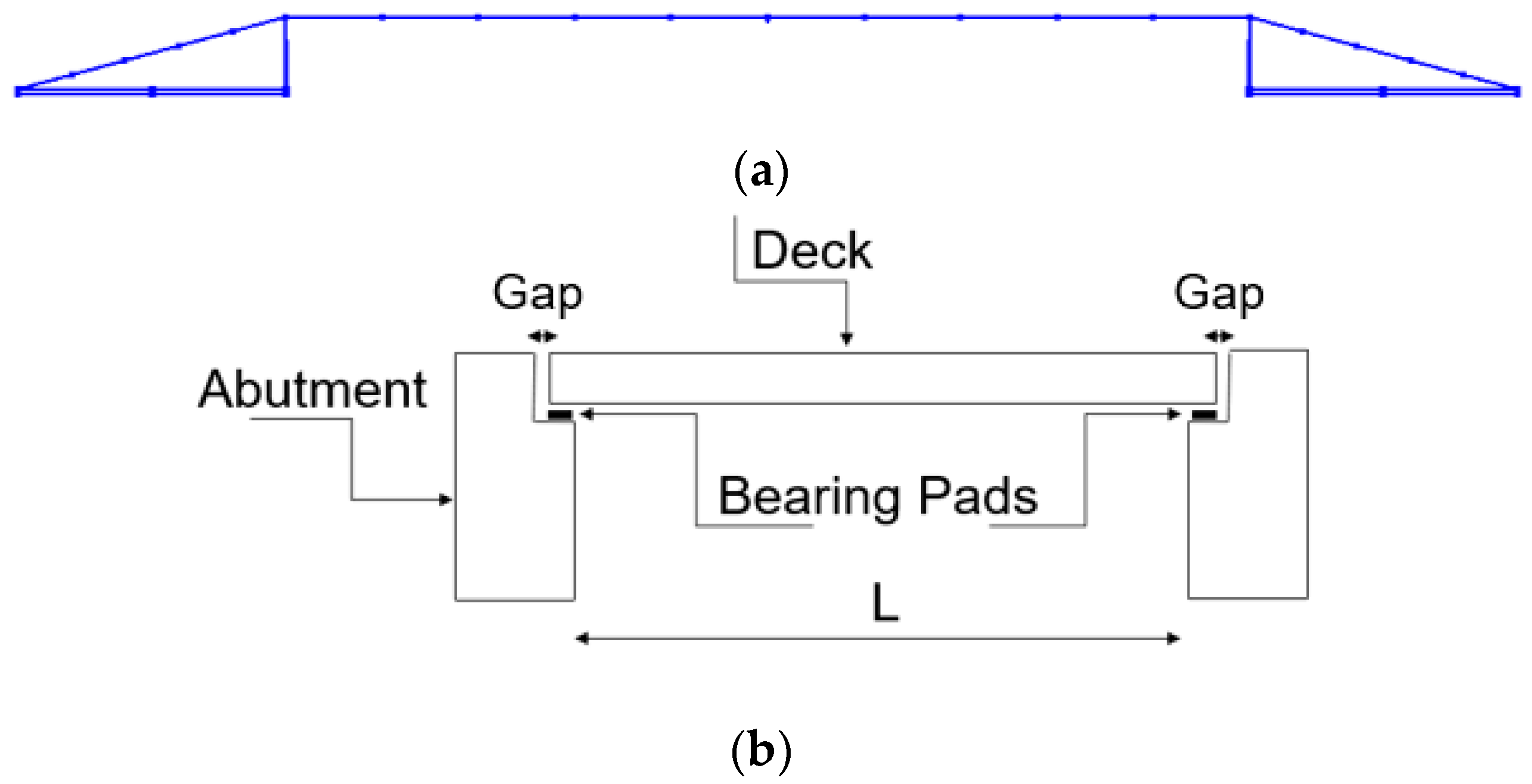
2.1. Bridge Model
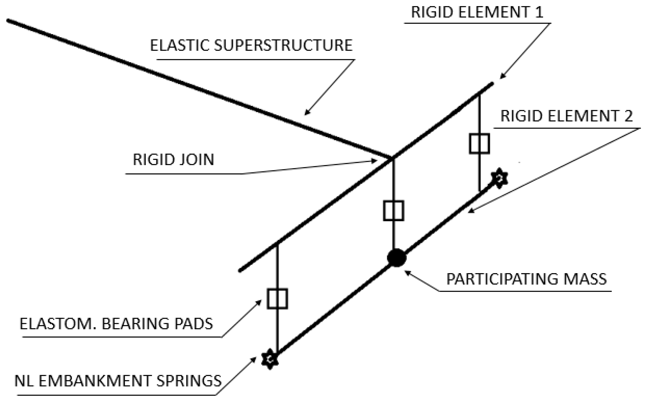
2.2. Abutment Model
- (1)
- the tributary weight of the superstructure and the effective abutment longitudinal stiffness were calculated to determine the structure period, T, using Equation C4.2.1-1 from [30]:
- (2)
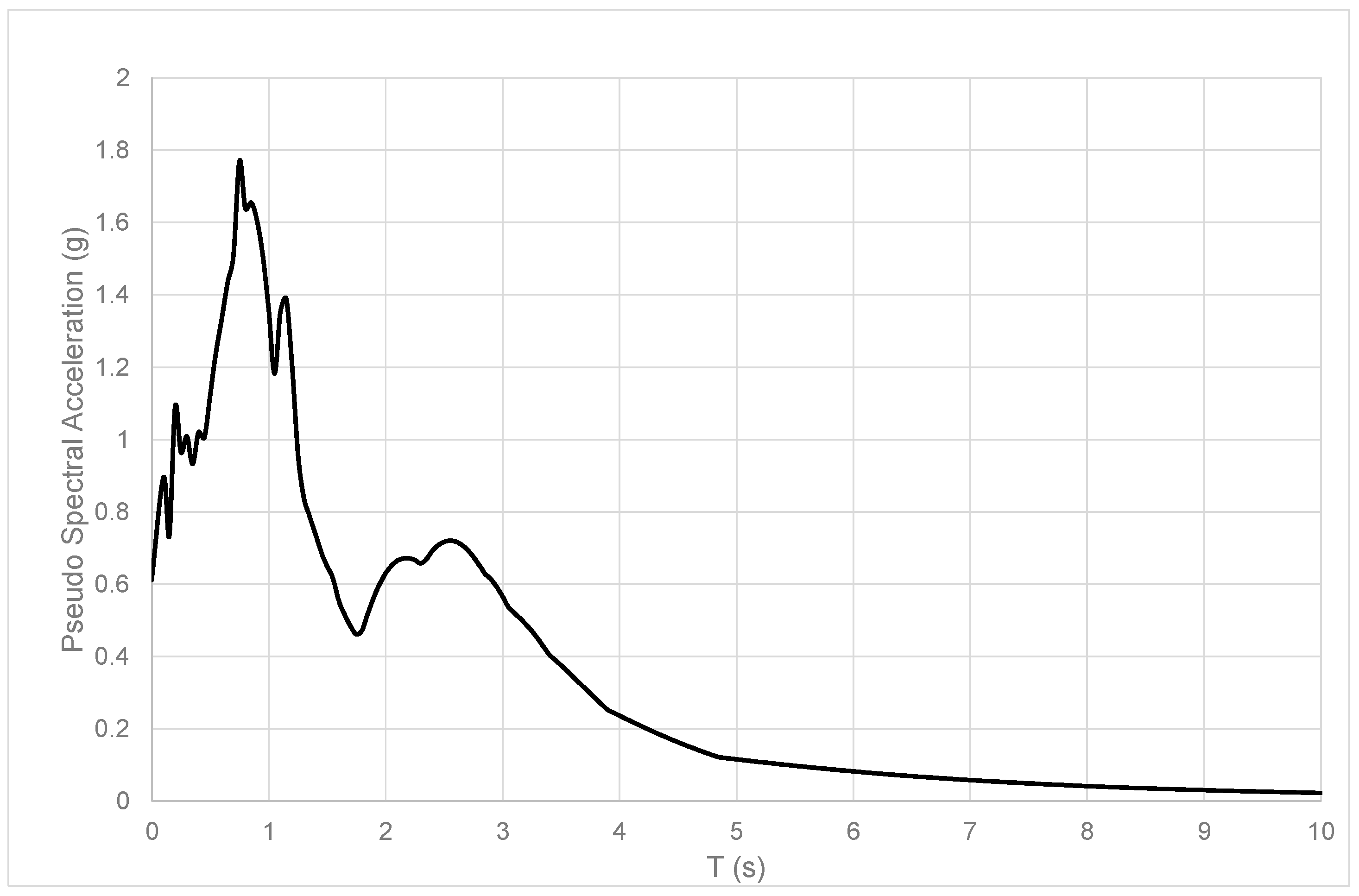
- The spectral acceleration (Sa), by introducing the period inside the design spectrum that was chosen as the maximum between the selected ones (SCS: PGA: 0612g; PGV: 116.85 cm/s and PGD: 54.19 cm, see Figure 3); and
- (3)
- The longitudinal displacement demand (∆D), which was determined from Equation 4.2.1-1 from [30]:
- needs to be taken as for seat abutments,
- needs to be taken as for seat abutments, and
- is taken as 1 for non-skew bridges.
3. Methodology
3.1. Seismic Scenario
- (1)
- Moment magnitude (Mw) 6.5–7.2 and closest distance (R) 15–30 km;
- (2)
- Mw 6.5–7.2 and R 30–60 km;
- (3)
- Mw 5.8–6.5 and R 15–30 km;
- (4)
- Mw 5.8–6.5 and R 30–60 km; and
- (5)
- Mw 5.8–7.2 and R 0–15 km.
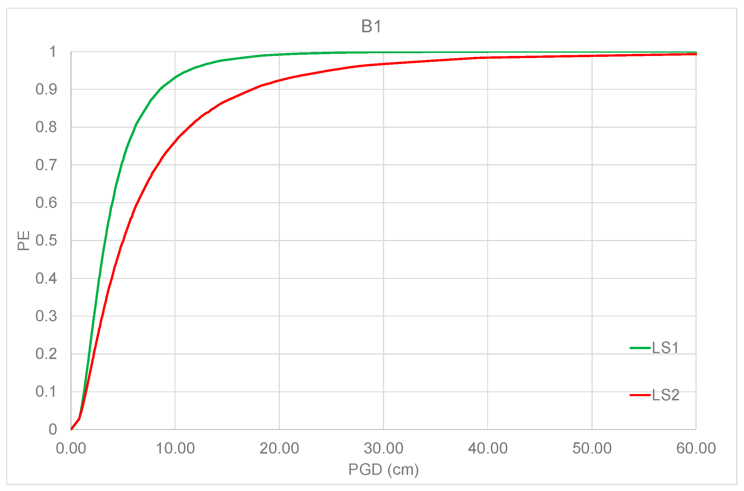
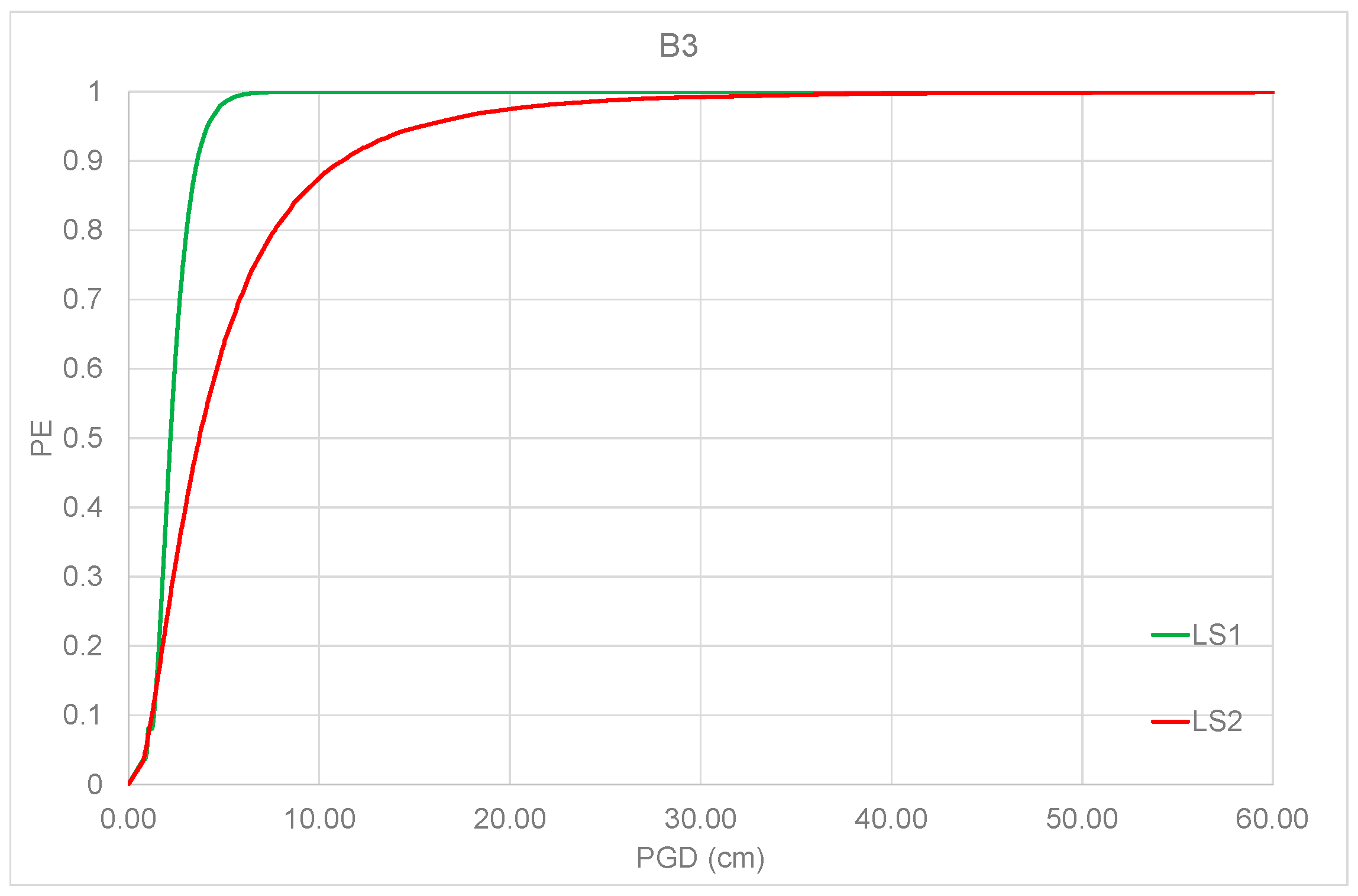
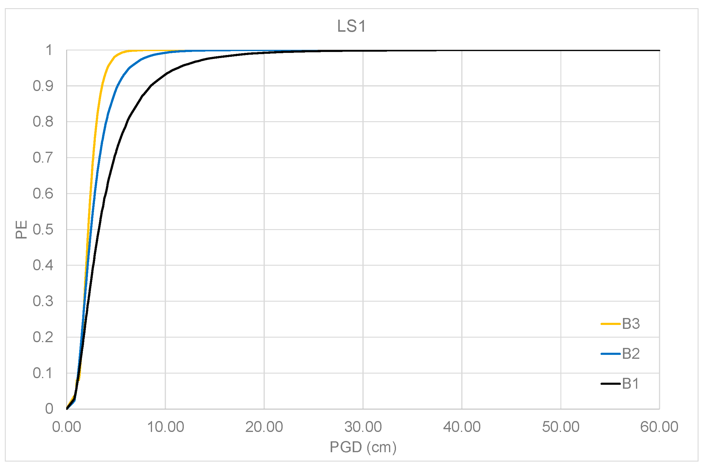
3.2. Fragility Curves
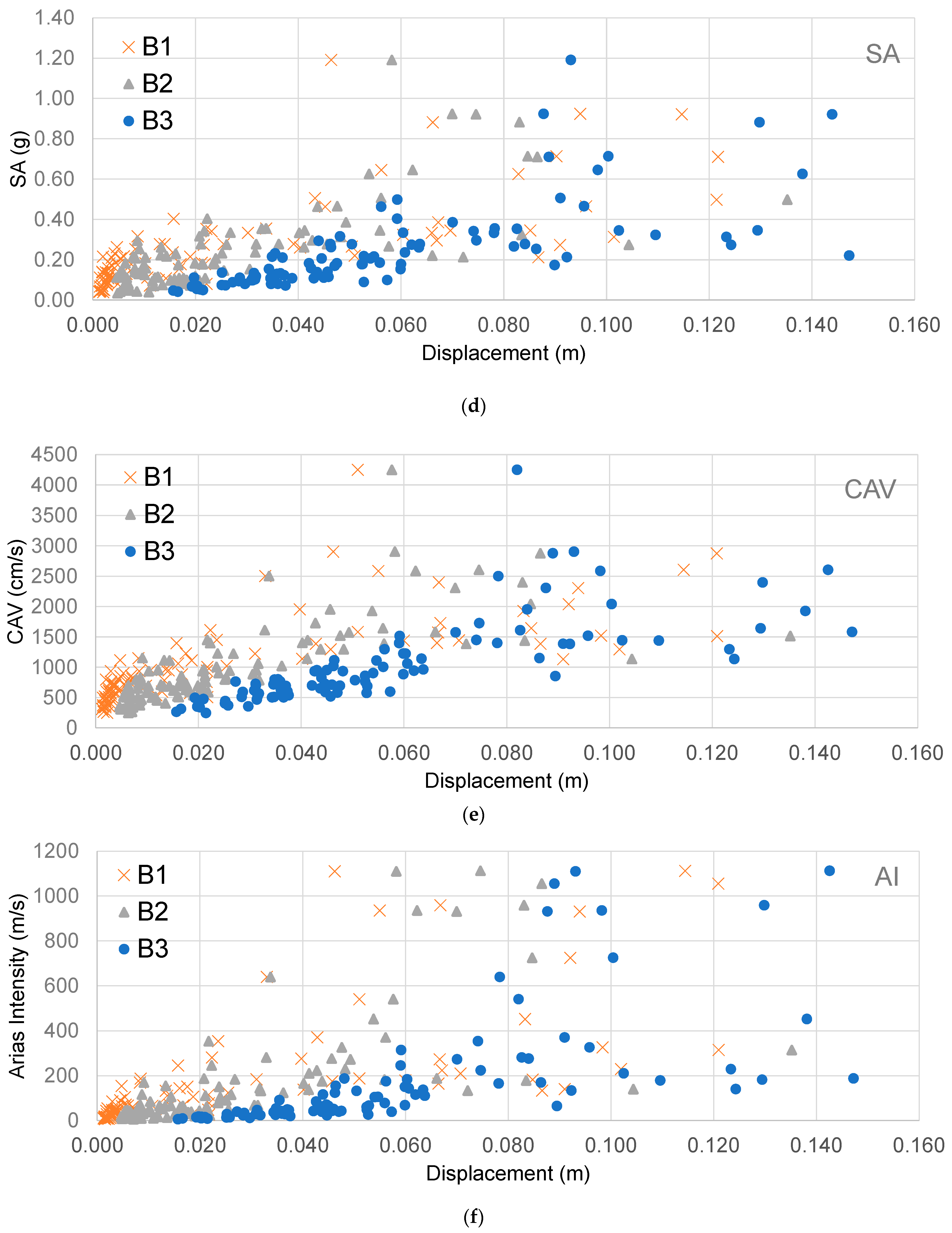
4. Results
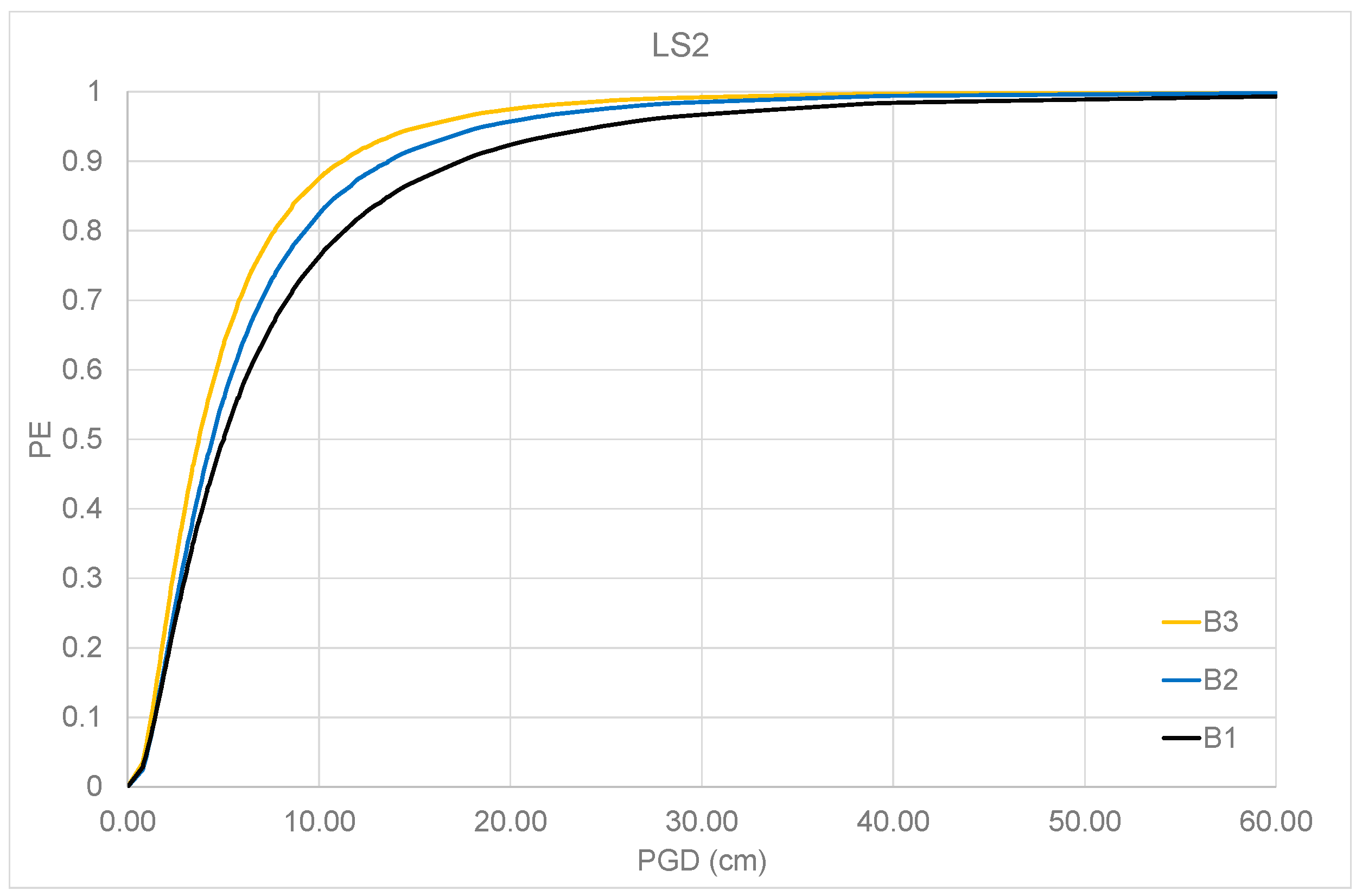
5. Analytical Fragility Curves
6. Conclusions
Funding
Institutional Review Board Statement
Informed Consent Statement
Data Availability Statement
Conflicts of Interest
References
- Gehl, P.; Seyedi, D.M.; Douglas, J. Vector-valued fragility functions for seismic risk evaluation. Bull. Earthq. Eng. 2013, 11, 365–384. [Google Scholar] [CrossRef]
- Sousa, L.; Silva, V.; Marques, M.; Crowley, H.; Pinho, R. Including multiple IMTs in the development of fragility functions for earthquake loss estimation. In Proceedings of the Vulnerability, Uncertainty, and Risk: Quantification, Mitigation, and Management, CDRM 9—American Society of Civil Engineers, Liverpool, UK, 13–16 July 2014; pp. 1716–1725. [Google Scholar]
- Padgett, J.E.; Nielson, B.G.; DesRoches, R. Selection of optimal intensity measures in probabilistic seismic demand models of highway bridge portfolios. Earthq. Eng. Struct. Dyn. 2008, 37, 711–726. [Google Scholar] [CrossRef]
- Zelaschi, C.; Monteiro, R.; Pinho, R. Critical assessment of intensity measures for seismic response of Italian RC bridge portfolios. J. Earthq. Eng. 2017, 23, 1342293. [Google Scholar] [CrossRef]
- HAZUS. Multi-Hazard Loss Estimation Methodology Earthquake Model; Federal Emergency Management Agency: Washington, DC, USA, 2003.
- Kohrangi, M.; Bento, R.; Lopes, M. Seismic performance of irregular bridges–comparison of different nonlinear static procedures. Struct. Infrastruct. Eng. 2015, 11, 1632–1650. [Google Scholar] [CrossRef]
- Pinho, R.; Marques, M.; Monteiro, R.; Casarotti, C.; Delgado, R. Evaluation of nonlinear static procedures in the assessment of building frames. Earthq. Spectra 2013, 29, 1459–1476. [Google Scholar] [CrossRef]
- Pinho, R.; Monteiro, R.; Casarotti, C.; Delgado, R. Assessment of continuous span bridges through nonlinear static procedures. Earthq. Spectra 2009, 25, 143–159. [Google Scholar] [CrossRef]
- Ebrahimian, H.; Jalayer, F.; Lucchini, A.; Mollaioli, F.; Manfredi, G. Preliminary ranking of alternative scalar and vector intensity measures of ground shaking. Bull. Earthq. Eng. 2015, 13, 2805–2840. [Google Scholar] [CrossRef]
- Giovenale, P.; Cornell, C.A.; Esteva, L. Comparing the adequacy of alternative ground motion intensity measures for the estimation of structural responses. Earthq. Eng. Struct. Dyn. 2004, 33, 951–979. [Google Scholar] [CrossRef]
- Bianchini, M.; Diotallevi, P.; Baker, J.W. Prediction of inelastic structural response using an average of spectral accelerations. In Proceedings of the 10th International Conference on Structural Safety and Reliability (ICOSSAR09), Osaka, Japan, 13–17 September 2009; p. 1317. [Google Scholar]
- Eads, L.; Miranda, E.; Lignos, D.G. Average spectral acceleration as an intensity measure for collapse risk assessment. Earthq. Eng. Struct. Dynam. 2015, 44, 2057–2073. [Google Scholar] [CrossRef]
- Biasio, M.D.; Grange, S.; Dufour, F.; Allain, F.; Petre-Lazar, I. A simple and efficient intensity measure to account for nonlinear structural behavior. Earthq. Spectra 2014, 30, 1403–1426. [Google Scholar] [CrossRef]
- Baker, J.W. Efficient analytical fragility function fitting using dynamic structural analysis. Earthq. Spectra 2015, 31, 579–599. [Google Scholar] [CrossRef]
- Baker, J.W.; Cornell, C.A. Vector-valued intensity measures incorporating spectral shape for prediction of structural response. J. Earthq. Eng. 2008, 12, 534–554. [Google Scholar] [CrossRef]
- Bayat, M.; Daneshjoo, F.; Nistico, N. A novel proficient and sufficient intensity measure for probabilistic analysis of skewed highway bridges. Struct. Eng. Mech. 2015, 55, 1177–1202. [Google Scholar] [CrossRef]
- Forcellini, D.; Alzabeebee, S. Seismic fragility assessment of geotechnical seismic isolation (GSI) for bridge configuration. Bull. Earthq. Eng. 2021. [Google Scholar] [CrossRef]
- Mackie, K.R.; Stojadinović, B. Performance-based seismic bridge design for damage and loss limit states. Earthq. Eng. Struct. Dyn. 2007, 36, 1953–1971. [Google Scholar] [CrossRef]
- Zentner, I. A general framework for the estimation of analytical fragility functions based on multivariate probability distributions. Struct. Saf. 2017, 64, 54–61. [Google Scholar] [CrossRef]
- Romstad, K.; Kutter, B.; Maroney, B.; Vanderbilt, E.; Griggs, M.; Chai, Y.H. Experimental Measurements of Bridge Abutment Behavior; Rep. No. UCD-STR-95-1; Department of Civil and Environmental Engineering, University of California: Davis, CA, USA, 1995. [Google Scholar]
- Bozorgzadeh, A. Effect of Backfill on Stiffness and Capacity of Bridge Abutments. Ph.D. Thesis, University of California, San Diego, CA, USA, 2007. [Google Scholar]
- Lemnitzer, A.; Ahlberg, E.; Nigbor, R.; Shamsabadi, A.; Wallace, J.; Stewart, J. Lateral Performance of Full-Scale Bridge Abutment Wall with Granular Backfill. J. Geotech. Geoenviron. Eng. 2009, 135, 506–514. [Google Scholar] [CrossRef]
- Mazzoni, S.; McKenna, F.; Scott, M.H.; Fenves, G.L. Open System for Earthquake Engineering Simulation, User Command-Language Manual; 2009; Available online: http://opensees.berkeley.edu/OpenSees/manuals/usermanual (accessed on 24 May 2022).
- Mina, D.; Forcellini, D. Soil–Structure Interaction Assessment of the 23 November 1980 Irpinia-Basilicata Earthquake. Geosciences 2020, 10, 152. [Google Scholar] [CrossRef]
- Forcellini, D. 3D Numerical simulations of elastomeric bearings for bridges. Innov. Infrastruct. Solut. 2016, 1, 1–9. [Google Scholar] [CrossRef]
- Forcellini, D. Assessment on geotechnical seismic isolation (GSI) on bridge configurations. Innov. Infrastruct. Solut. 2017, 2, 1–6. [Google Scholar] [CrossRef]
- Lam, I.; Martin, G.R. Seismic Design of Highway Bridge Foundations; U.S. Department of Transportation, Federal Highway Administration, Research, Development, and Technology: Washington, DC, USA, 1986.
- Aviram, A.; Mackie, K.R.; Stojadinovic, B. Effect of abutment modeling on the seismic response of bridge structures. Earthq. Eng. Eng. Vib. 2008, 7, 395–402. [Google Scholar] [CrossRef]
- Kotsoglu, A.; Pantazopoulou, S. Modeling of Embankment Flexibility and Soil-structure Interaction in Integral Bridges. In Proceedings of the First European Conference on Earthquake Engineering and Seismology, Geneva, Switzerland, 3–8 September 2006. [Google Scholar]
- Caltrans. Caltrans Seismic Design Criteria; Version 2.0; California Department of Transportation; Sacramento, CA, USA, 2019. [Google Scholar]
- Zhang, J.; Makris, N. Kinematic Response Functions and Dynamic Stiffnesses of Bridge Embankments. Earthq. Eng. Struct. Dyn. 2002, 31, 1933–1966. [Google Scholar] [CrossRef]
- Werner, S.D. Study of Caltrans’ Seismic Evaluation Procedures for Short Bridges. In Proceedings of the 3rd Annual Seismic Research Workshop, Sacramento, CA, USA, 27–29 June 1994. [Google Scholar]
- Gupta, A.; Krawinkler, H. Estimation of seismic drift demands for frame structures. Earthq. Eng. Struct. Dyn. 2000, 29, 1287–1305. [Google Scholar] [CrossRef]
- Mackie, K.R.; Wong, J.-M.; Stojadinovic, B. Integrated Probabilistic Performance-Based Evaluation of Benchmark Reinforced Concrete Bridges; Report No. 2007/09; Pacific Earthquake Engineering Research Center, University of California: Berkeley, CA, USA, 2007. [Google Scholar]
- Forcellini, D. Cost assessment of isolation technique applied to a benchmark bridge with soil structure interaction. Bull. Earthq. Eng. 2017, 15, 51–69. [Google Scholar] [CrossRef]
- Mina, D.; Forcellini, D.; Karampour, H. Analytical fragility curves for assessment of the seismic vulnerability of HP/HT unburied subsea pipelines. Soil Dyn. Earthq. Eng. 2020, 137, 106308. [Google Scholar] [CrossRef]


| L (ft) | L (m) | A (m2) | ITR (m4) | ILG (m4) | |
|---|---|---|---|---|---|
| B1 | 40 | 12.19 | 3.36 | 1.65 | 31.71 |
| B2 | 60 | 18.29 | 3.46 | 1.70 | 32.56 |
| B3 | 80 | 24.38 | 3.61 | 1.77 | 33.97 |
| Bearing Pads: Properties | Values |
|---|---|
| Number | 3 |
| Height (m) | 0.05 |
| Shear modulus G (kPa) | 1034 |
| Young modulus E (kPa) | 34,474 |
| Yield displacement (%) | 150 |
| Ultimate displacement (%) | 300 |
| W (kN) | T (s) | K (kN/m) | Sa | ||
|---|---|---|---|---|---|
| B1 | 935 | 0.185 | 11,500 | 1.01 | 0.0086 |
| B2 | 1440 | 0.245 | 96,450 | 0.97 | 0.0144 |
| B3 | 2000 | 0.360 | 62,300 | 0.93 | 0.0230 |
| h (ft) | w (ft) | Fbw | kabut | RA | ||||
|---|---|---|---|---|---|---|---|---|
| B1 | 1.3 | 92 | 239 | 2498 | 0.096 | 0.0254 | 0.121 | 0.07 |
| B2 | 1.4 | 95 | 281 | 2632 | 0.106 | 0.0254 | 0.132 | 0.109 |
| B3 | 1.5 | 100 | 333 | 2825 | 0.118 | 0.0254 | 0.143 | 0.209 |
| R2 | PGA | PGV | PGD | SA | CAV | AI |
|---|---|---|---|---|---|---|
| B1 | 0.5204 | 0.7022 | 0.7349 | 0.5261 | 0.5164 | 0.4783 |
| B2 | 0.4903 | 0.7007 | 0.8646 | 0.5002 | 0.5050 | 0.4526 |
| B3 | 0.4486 | 0.6927 | 0.8025 | 0.4887 | 0.5383 | 0.4321 |
| LS1 | Ratio (%) | LS2 | Ratio (%) | |
|---|---|---|---|---|
| B1 | 0.935 | 93.45 | 0.767 | 87.30 |
| B2 | 0.993 | 99.30 | 0.829 | 94.30 |
| B3 | 0.999 | 100 | 0.879 | 100 |
Publisher’s Note: MDPI stays neutral with regard to jurisdictional claims in published maps and institutional affiliations. |
© 2022 by the author. Licensee MDPI, Basel, Switzerland. This article is an open access article distributed under the terms and conditions of the Creative Commons Attribution (CC BY) license (https://creativecommons.org/licenses/by/4.0/).
Share and Cite
Forcellini, D. Assessment of the Seismic Vulnerability of Bridge Abutments with 3D Numerical Simulations. Geosciences 2022, 12, 316. https://doi.org/10.3390/geosciences12090316
Forcellini D. Assessment of the Seismic Vulnerability of Bridge Abutments with 3D Numerical Simulations. Geosciences. 2022; 12(9):316. https://doi.org/10.3390/geosciences12090316
Chicago/Turabian StyleForcellini, Davide. 2022. "Assessment of the Seismic Vulnerability of Bridge Abutments with 3D Numerical Simulations" Geosciences 12, no. 9: 316. https://doi.org/10.3390/geosciences12090316
APA StyleForcellini, D. (2022). Assessment of the Seismic Vulnerability of Bridge Abutments with 3D Numerical Simulations. Geosciences, 12(9), 316. https://doi.org/10.3390/geosciences12090316