Abstract
When conducting numerical upscaling, either for a fractured or a porous medium, it is important to account for anisotropy because in general, the resulting upscaled conductivity is anisotropic. Measurements made at different scales also demonstrate the existence of anisotropy of hydraulic conductivity. At the “microscopic” scale, the anisotropy results from the preferential flatness of grains, presence of shale, or variation of grain size in successive laminations. At a larger scale, the anisotropy results from preferential orientation of highly conductive geological features (channels, fracture families) or alternations of high and low conductive features (stratification, bedding, crossbedding). Previous surveys of homogenization techniques demonstrate that a wide variety of approaches exists to define and calculate the equivalent conductivity tensor. Consequently, the resulting equivalent conductivities obtained by these different methods are not necessarily equal, and they do not have the same mathematical properties (some are symmetric, others are not, for example). We present an overview of different techniques allowing a quantitative evaluation of the anisotropic equivalent conductivity for heterogeneous porous media, via numerical simulations and, in some cases, analytical approaches. New approaches to equivalent permeability are proposed for heterogeneous media, as well as discontinuous (composite) media, and also some extensions to 2D fractured networks. One of the main focuses of the paper is to explore the relations between these various definitions and the resulting properties of the anisotropic equivalent conductivity, such as tensorial or non-tensorial behavior of the anisotropic conductivity; symmetry and positiveness of the conductivity tensor (or not); dual conductivity/resistivity tensors; continuity and robustness of equivalent conductivity with respect to domain geometry and boundary conditions. In this paper, we emphasize some of the implications of the different approaches for the resulting equivalent permeabilities.
1. Introduction
The hydraulic conductivity of geological media is often anisotropic as it has been shown in laboratory and field experiments on a wide variety of scales and a wide variety of porous or fractured rocks [1,2,3,4,5,6,7,8,9,10,11,12,13]. At the microscopic (pore) scale, the anisotropy is due to the preferential flatness of grains, the presence of shale, or the variation of grain size in successive laminations. At a larger scale, the anisotropy results from preferential orientation of geological features such as fracture families, stratifications, or channels [14,15]. Anisotropy is a key parameter controlling the behavior of solutes such as contaminants in porous materials [16,17]. An example demonstrating the crucial importance of anisotropy for regional hydrogeology studies is the study of Arsenic contamination in the Bengal basin [18]. Anisotropy can trigger the existence of groundwater whirls [19,20] that may have a large influence on reactive transport and dilution processes. Anisotropy can impact the efficiency of greenhouse gases (such as CO2), sequestration in deep geological formations [21], and heat extraction by geothermal boreholes [22].
Therefore, there is a need for methods and tools allowing to estimate anisotropy in the laboratory [23,24,25,26] or in the field [27,28,29], or to evaluate anisotropy through upscaling techniques (e.g., when a detailed geological model has been built but is too detailed for direct numerical modeling). When anisotropy is put in this perspective, one realizes that some common techniques can be used to interpret permeametric experiments in the laboratory as well as numerical experiments based on geological models.
Those techniques have been essentially developed over the last 50 years in the framework of upscaling, either on finite domains or finite “blocks” (equivalent block conductivity, as in the present work) or in infinite domain (effective hydraulic conductivity). Analyses and reviews of these methods can be found, for example, in [30,31,32,33,34,35,36]. Their applications to estimate tensorial permeabilities in numerical experiments or in the laboratory have been studied by many authors (including, for example, [23,25,37,38,39,40,41,42,43,44]. Other works have focused on optimal estimation of heterogeneous reservoir properties such as permeability . For instance, techniques such as truncated Proper Orthogonal Decomposition (POD) have been used in this context, as well as High Order Singular Value Decompositions (HOSVD), which lead typically to a coarsened optimal estimation of permeability distribution (e.g., [45]). Other orthogonal decompositions such as wavelet decompositions have been used for intermediate upscaling of permeability with application to solute transport upscaling (e.g., [46]).
Note that within the upscaling literature, one can distinguish effective properties and equivalent block properties. The effective properties emerge when the size of the heterogeneities is much smaller than the size of the sample and when there is some statistical homogeneity within the sample or some geometrical periodicity. When these conditions are not met, the equivalent conductivity is not any more an intrinsic property of the medium, and to avoid confusion with effective permeability one uses, in general, terminology such as equivalent block permeability, or simply block permeability. In the following, we will consider only block permeability tensors. The two concepts converge when the conditions of emergence of an effective permeability are met.
The block hydraulic conductivity, or block permeability tensor, obtained from an experiment (either numerical or physical) can be very different depending on the technique used to analyze the experiment (type of averaging, for example) and on the type of experiment itself (essentially the type of boundary conditions imposed on the sample). This is especially the case if the porous sample exhibits anisotropic heterogeneity features having a scale comparable to the size of the sample. This effect is described in most of the reviews cited above, and in several other papers [39,43,47,48,49,50,51,52].
In particular, it is known that depending on the technique used, one can obtain non-symmetrical tensors (e.g., [53,54,55]. This has raised controversial issues. For example, if the hydraulic conductivity tensor is not symmetric, it implies that there is no direction such that the Darcy velocity is parallel to the hydraulic gradient, and one cannot identify anymore the usual principal directions of anisotropy. Note, however, that it is possible to analyze a non-symmetric permeability tensor in terms of two sets of principal directions and principal components.
Similarly, it is possible to obtain tensors that may not be positive definite. For instance, the permeability tensor may be indefinite; or else it may be semi-definite positive (i.e., positive in some directions but zero in some other directions). In the most counter-intuitive situations, one can obtain a permeability tensor having one negative eigenvalue, that is, a negative principal permeability (see example in Section 6.2). This implies that the mean flow along this principal direction will go “upgradient”, from zones of low hydraulic head to zones of high hydraulic head. In addition, if the permeability tensor is not definite positive, it implies that there may be some directions of flow such that the energy dissipated by the viscous forces in the medium can become zero or even negative (a situation that has no physical sense). Indeed, the only way to ensure that the dissipated power is always strictly positive when the head gradient is not equal to zero is to ensure that the permeability tensor is definite positive.
To better understand the relations between the definitions and properties of the permeability tensors obtained from upscaling procedures or averaging techniques in numerical or laboratory experiments, we present an overview of the most frequent techniques, and we discuss new approaches as well. Specifically, the main focus of this work is to explore the relations between these various definitions and the resulting properties of the anisotropic equivalent conductivity.
Fracture networks constitute a special case of interest [40,51,56,57,58,59,60]. If the porous matrix is assumed impervious, then flow takes place only through an intersecting network of discrete conductive objects (the percolating subset of the fracture network). If the network is considered to be 2D, then flow occurs through a bond network of links and nodes (or its percolating subset). An algebraic approach to the equivalent permeability of such a 2D network was proposed by Ababou and Renard [61,62]. The case of 3D planar fractures is more complex. The percolating subset and other properties of a 3D network of planar disc fractures were analyzed recently by Cañamón et al. [63]. In these works, the rock matrix was assumed impervious, and the emphasis was on the topological graph properties of the fracture networks. Additionally, because of this extreme type of discontinuity (flowing fractures vs. impervious matrix), it is often necessary to use special dedicated formulations for flux averages and equivalent conductivities. The intermediate case of a 3D permeable rock matrix traversed by planar disc fractures was also treated by Rajeh, Ababou et al. [64]; their study of permeability upscaling took into account both the permeability contrast Kf/Km and the density of the 3D fracture set. They also considered the asymptotic case Kf/Km → ∞, and they finally expressed the upscaled tensorial permeability of the matrix/fracture medium in terms of a critical density of fractures (the so-called critical “exclusion density” based on the exclusion volume of fractures). Other works that focus on fractured media include Long [40], Pouya and Fouché [43], and Lang et al. [39]. Barker et al. [65] consider the spectral graph properties of networks and developed a reservoir simulation application involving a Finite Volume discretization of a 3D heterogeneous continuum, re-interpreted as a 3D network of links.
In the following, we consider three types of heterogeneous media:
- continuous porous media: this includes the special cases of uniform (homogenous) media, non-uniform (inhomogeneous) media with continuously varying properties, and spatially correlated random media;
- composite porous media: this includes various multilayered media, as well as more general Boolean porous media (binary random mixtures, thresholded random fields, etc.) where permeability is non-zero everywhere;
- fractured networks: we include in this category the special case of 2D fractured media with impervious porous matrix; this case is equivalent to the problem of flow on a network.
In the remainder of this work, we focus to a larger extent on the first two types of heterogeneous media mentioned above: (i) continuous porous media, and (ii) composite porous media, and to a lesser extent on the third case (iii) of fractured media/2D networks.
The remainder of this paper is organized as follows:
In the next section (Section 2), we present our assumptions of flow and geometry, and we show how the conductivity tensor can be computed from the results of numerical experiments. This requires that one defines both the boundary conditions (experimental setup) and the equivalence criteria to be used to define the equivalent conductivity, usually through some kind of averaging. In Section 3, we present some special analytical solutions for Darcy flow in finite domains, which provide insights on the effects of permeability variability on the flow pattern and can sometimes lead to analyses of the corresponding equivalent permeability tensor. In Section 4, various average quantities and equivalence criteria are proposed to define and calculate the equivalent hydraulic conductivity of heterogeneous blocks. Combining these average quantities and criteria with various types of boundary conditions or flow experiments leads to several different ways of calculating the equivalent permeability tensor. In Section 6, numerical experiments are implemented on 10 samples of heterogeneous porous media, including continuously variable random field conductivity patterns, as well as composite or random Boolean conductivity patterns. The special case of 2D fracture networks is treated separately, analytically, in Section 6.2. Section 7 presents analytical and algebraic proofs concerning the properties of equivalent conductivity tensors obtained by some of the previous methods, and the relations between the different methods. A brief conclusive section is provided in Section 8. It is followed by several Appendices, which complete some of the developments presented in the text concerning heterogeneous flow patterns, averages, boundary conditions, etc.
2. Definitions and Assumptions on Flow and Geometry
Defining upscaling techniques and characterizing their properties requires first defining the following items: the local flow model; the global or upscaled flow model; a formal or general definition of the upscaled permeability tensor; a series of (possibly alternative) equivalence criteria or homogenization criteria; and a description of the boundary conditions used to calculate the equivalent permeability or conductivity tensor. Note: a brief introduction to tensorial permeability will be presented in Section 2.4, with more details in Appendix A.1, concerning second rank tensors in general, then conductivity tensors in particular, ending up with the concept of directional conductivity (when flow is governed by the tensorial form of Darcy’s law).
2.1. Flow Domain: Block Geometry
We do not fix a priori the geometry of the domain of interest. It can either be a simple geometrical shape (rectangle, parallelepiped, triangle, tetrahedron, etc.) or completely general. In some situations, we may have to use a parallelepipedic geometry. In such a case, we will use the conventions introduced in Figure 1.
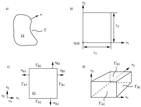
Figure 1.
Geometrical sketch of: (a) a general 2D domain Ω, with n the outgoing normal vector with respect to the boundary Γ. (b) Rectangular domain geometry and size. (c) Faces and normal vectors in a rectangular geometry. The letter A stands for the faces closest to the origin. The letter B corresponds to the opposite face. The index (1,2, or 3) stands for the axis perpendicular to the face. (d) The same principle is used to denote the faces of a 3D parallelepipedic domain as well.
2.2. Local Flow Models
At the macroscopic scale, the distribution of permeability within the porous medium (or the spatial distribution of the fractures and their apertures) is assumed to be known. The geometry of the domain is also assumed to be known. Note: in the case of a fractured porous medium, we would consider two local flow models, one for the porous medium and one for the fractures; however, here we only provide indications for the case of 2D fracture networks neglecting the permeability of the porous matrix.
2.2.1. Head-Based Flow Equations for a Porous Medium
The porous medium is assumed to be water-saturated (or liquid saturated more generally). The flow is assumed to follow Darcy’s law:
where v(x) [LT−1] is the local Darcy velocity vector or specific discharge (often denoted q(x)); h [L] is the local total hydraulic head, and k(x) [LT−1] is the local hydraulic conductivity tensor, which is assumed symmetric and positive-definite [66,67].
Note that the local, “hydraulic gradient” is often defined as in the literature, so that Darcy’s law can also be expressed as .
In addition, the Darcy velocity obeys a steady state mass conservation equation (assuming here incompressible fluid):
Finally, the local head-based flow equation is obtained by inserting Darcy’s law Equation (1) into Equation (3):
In what follows, we will usually assume that the local conductivity is isotropic; therefore k(x) is a spatially distributed scalar rather than a tensor (locally). (In the remainder of this paper, we use interchangeably the terms “permeability” and “hydraulic conductivity” for convenience, although strictly speaking, k & K represent here local & block scale hydraulic conductivity [m/s].) The local total hydraulic head h [L] is defined as the sum of pressure potential plus gravitational potential, converted into water column height as follows:
where is the vertical elevation (pointing upwards), is pore water pressure, is air pressure (atmospheric), is the acceleration of gravity, and is the density of liquid water (or the density of the incompressible liquid that saturates the porous medium).
2.2.2. Velocity-Based Flow Equations for a Porous Medium
Alternatively, a “flux”-based flow equation governing directly the Darcy velocity in a heterogeneous porous medium has been proposed ([68] Section 4.3 therein, [69] Section 3.5 therein). This equation is obtained by re-stating Darcy’s law Equation (1) as follows and assuming from now on that the local permeability is isotropic (scalar field ):
We can then infer that the curl of must be null because the curl of a gradient is always null. By definition, the curl (rotational) of a vector field is the vector product (or cross product) of the vectorial operator with vector . The velocity equation (which is a direct consequence of Darcy’s law) is given by:
Finally, this rotational Equation (7), together with the divergence Equation (3), form a velocity-based system of vector equations, which can be used to solve directly for the velocity field instead of the head-based Equation (5). Once solved, the hydraulic gradient can then be obtained from Equation (6), and the scalar head field can then be obtained by integration from any boundary point where the head is prescribed.
A more detailed derivation of these velocity or flux-based equations is presented later below in Section 3.1 and in Appendix A.2. In the case of randomly heterogeneous media, the consequences of these local velocity-based equations, as opposed to head-based equations, were studied by Akpoji et al. [70].
The main consequence of this alternative formulation, in the context of equivalent permeability, is that the averaged version of this flow equation may not yield the same equivalent permeability as the head-based flow equations (see discussion in Section 2.3).
2.2.3. Head-Based Flow Equations for a 2D Fracture Network (Indications)
In the fractures, the flow is assumed to follow a linear law such as the cubic law. In two dimensions, the fracture network is represented by a graph [71,72] of edges and nodes (as shown in Figure 2).
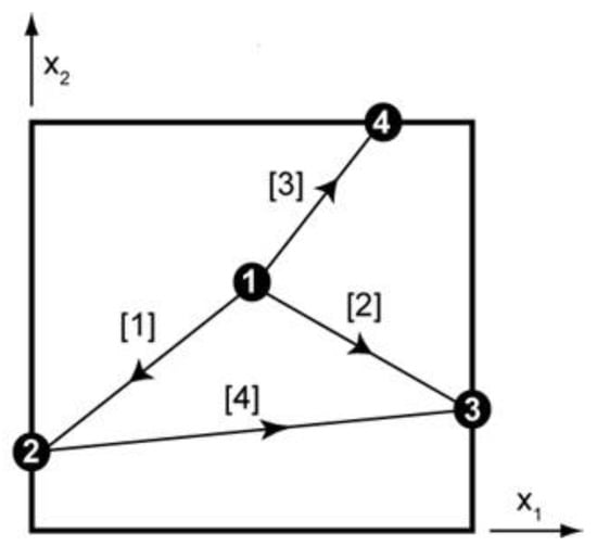
Figure 2.
Example of a simple 2D fracture network, represented by a directed graph (“digraph”). Black circles such as  represent the vertices of the graph (i.e., the nodes of the intersecting fracture network), and the line segments with numbers [2] represent the “arcs” or “edges” of the graph (i.e., the fracture segments or links between nodes). The links are interconnected to each other via vertices (nodes). The vertices can be numbered in any order, and similarly for the edge numbers. For a fracture network, the edge directions can also be set up using any predefined convention (see text).
represent the vertices of the graph (i.e., the nodes of the intersecting fracture network), and the line segments with numbers [2] represent the “arcs” or “edges” of the graph (i.e., the fracture segments or links between nodes). The links are interconnected to each other via vertices (nodes). The vertices can be numbered in any order, and similarly for the edge numbers. For a fracture network, the edge directions can also be set up using any predefined convention (see text).
The flux qi [LT−3] along the edge “” is also denoted vi for convenience (being similar to a velocity). It is modeled according to either Darcy’s law or Poiseuille’s law, by:
with [L2T−1] the conductance of edge “”, hj and hk [L] the hydraulic heads at the nodes corresponding to the extremities of edge “”, li the distance between the two end-nodes of edge “”. Note that we have used here the single index “” to label the edges or links, and the double index to label their two end-nods. Alternatively, it is possible to use the double index to label conductivities (e.g., ) and conductances (e.g., ) of the fracture kinks .
The conservation equation is then written for each node of the graph. This law (known as Kirchhoff’s law) states that the balance of the fluxes of all the edges connected to a given node is equal to zero (zero net flux at any given node):
where represents the indices k of all nodes connected to the node j by a fracture link (j,k). For example, in a regular hexagonal network, each node has six neighbors, and the Kirchhoff law above expresses that, at any node of the network, the sum of all six velocities (ingoing and outgoing) must be zero.
2.3. Upscaled Flow Model with Equivalent Conductivity
It is assumed that both in the case of a fractured or a porous medium, the large-scale flow can be described by a macroscopic model analogous to the local Darcy and mass conservation equations, but with macroscale or block scale quantities (we use capital letters for these macroscale quantities):
hence, the head-based flow equation is obtained by inserting Darcy’s law Equation (10) into Equation (12):
In these macroscale equations, [LT−1] is the upscaled or equivalent hydraulic conductivity (possibly non-symmetric), [L] is the macroscale hydraulic head within the upscaled block, and is the macroscale specific discharge (Darcy velocity). The macroscale “hydraulic gradient” is defined as .
In all cases, it is assumed that the macroscale V, , or J are continuous and smoothly varying functions within the domain. We will assume in many cases that the macroscale quantities , , and can be considered spatially constant within the block (although this is not necessary), and in such cases, the macroscale head is a linear function of space. In particular, note that the macroscale velocity is either constant or smoothly varying, while in contrast, the local Darcy velocity vector can be highly variable and even discontinuous, for instance in composite or fractured media where the tangential component of can be discontinuous across a fracture or a material discontinuity within the block. Finally, note also that K, V, are not necessarily defined as simple arithmetic averages of the local variables , ,.
Several authors, including ([30,73,74], [68] Chapter 4 therein), and others, have demonstrated that such a model governs the large-scale flow if the following conditions are met:
- the heterogeneities have a small size compared to domain size (or, for a random medium, the spatial correlation scales of the medium are small with respect to domain size, which is analogous to the theoretical “infinite domain” hypothesis); and
- the flow field is “homogeneous” at the macro-scale or domain scale (or, in the case of a random medium, the flow field should be statistically homogeneous up to second order).
However, when dealing with practical situations, the previous conditions may not be fulfilled. For instance, the mean large-scale flow could be radial, as would occur around a pumping well, or the heterogeneous structures of the medium could be as large as the size of the sample. If this would be the case, implementing the simplified macroscopic phenomenological law of Equations (10) and (12) with constant K, V, would be mistaken, because we know it is not theoretically exact when the cited conditions on inhomogeneity and/or scales are not met.
As mentioned in Section 2.2.2, the averaged velocity-based flow equations may not yield the same equivalent permeability as the head-based flow equations. For instance, the velocity version of Darcy’s law, Equation (7), may lead, upon averaging, more naturally, to an equivalent resistivity (rather than an equivalent permeability). The challenge is then to match the equivalent permeability (obtained from head-based equations) to equivalent resistivity (obtained from velocity-based equations). We refer to Fadili and Ababou [75] for a similar dual permeability-resistivity upscaling approach in the context of randomly heterogeneous media for single-phase and two-phase flow. A more general matching procedure could be attempted for arbitrarily heterogeneous porous and/or fractured blocks, but this possible extension will not be developed further here.
2.4. Tensorial Conductivity & Directional Conductivity Ellipse
This sub-section presents brief definitions of second rank tensors (such as the conductivity tensor ) and several related concepts: principal axes, principal values, directional “flux” and “gradient” conductivities, anisotropic conductivity ellipses. This topic is relevant for both microscale (local) and macroscale (upscaled) flow models. For references, see [76] concerning vectors and tensors in fluid mechanics, and [77] concerning principal and directional conductivities. A more detailed presentation of the algebraic aspects of this subsection can be found in Appendix A.1.
2.4.1. Vectors, Second Rank Tensors, and Tensorial Conductivity
Vectors, Tensors, and Transformation Rules
A vector is a first rank tensor. A second rank tensor or can be viewed as a linear application and can be represented by a matrix, for instance (in 2D with N = 2):
The coefficients depend on the system of coordinates , and the change if the system is changed by a rotation , or conversely its transpose , which transforms the new system into the initial system and is called the passage matrix . The rotation matrix and the passage matrix are orthogonal: (identity matrix).
The transformation rule for a vector under a change of coordinate system, that is, under a rotation of the basis vectors , is as follows, in terms of the passage matrix :
The quantity is a “true” vector only if it is transformed as shown above under a rotation of the coordinate system. Otherwise, it is not a true vector (it is, rather, a pseudo-vector).
Finally, the transformation rule for a second rank tensor under a rotation of the basis vectors is as follows, in terms of the passage matrix :
(summation on repeated indices)
Application to Darcy’s Law with Anisotropic Tensor
Darcy’s law is , where the Darcy velocity vector , the head gradient vector , and the conductivity tensor are all expressed in the reference system . The notation is also used to designate the hydraulic gradient and will be used elsewhere.
We now derive the expression of Darcy’s law in a new transformed system as follows. We start with Darcy’s law in the reference system ; we insert the vector transformation rules and ; and we also insert the tensor transformation rule . This yields:
which is just Darcy’s law in the new system , with the transformed conductivity as expected.
Principal System, Diagonalization
The transformation rules serve in particular for finding the principal vectors and the principal permeability values ( without summation). In the new principal system , the conductivity tensor is expressed by a diagonal matrix with real non-negative values. Briefly:
The first equation has three positive real roots () if is symmetric positive definite; the second equation consists of solving for the three principal vectors once the eigenvalues () are known. The principal basis vectors , or eigenvectors, are the column vectors of the passage matrix that takes the new principal basis into the initial basis (such that ). In the principal basis, tensor is represented by a diagonal matrix with . The conductivity matrix in any given coordinate system can always be expressed in terms of the diagonalized matrix using the relation , where contains the ’s as column vectors. More details in Appendix A.1.1 concerning the principal values and axes for the 2D case.
Note: the above description concerns the diagonalization of a symmetric positive definite tensor. (For a non-symmetric tensor, there are two distinct principal bases and two distinct sets of principal values.)
2.4.2. Directional Conductivity and Conductivity Ellipse
If is a second rank tensor, symmetric and positive definite (this applies also to non-symmetric if its symmetric part is definite positive), then it can also be described equivalently in the form of a directional conductivity parallel to flux , or parallel to hydraulic gradient . These are functions of the direction of Darcy velocity or of the gradient , respectively. Direction angles can be used: polar angle θ in 2D; spherical angles (θ, ϕ) in 3D. It can be shown that the polar plots of these directional conductivities (or their square roots) describe an ellipse in 2D, or an ellipsoid in 3D. The conductivity ellipse contains all the information about the tensor: the principal diameters are related to the principal values of , and the principal axes of the ellipse coincide with the principal vectors of .
Directional Conductivity
Let us start again with the tensorial form of Darcy’s law, using the notation :
Let be the unit “flux” vector (aligned with Darcy velocity); then by definition: . Similarly, let be the unit “gradient” vector (aligned with ); then by definition: . The directional “flux” conductivity () is a scalar quantity obtained by “projecting” Darcy’s law on the direction of the “flux”, as follows:
Similarly, the directional “gradient” conductivity () is a scalar quantity obtained by “projecting” Darcy’s law on the direction of the “gradient”, as follows:
Anisotropic Conductivity Ellipse
By re-inserting Darcy’s law with tensorial conductivity, and noting that and it can be shown that [40,77]:
In 2D, let and designate the polar angles of the “flux” (Darcy velocity) and of the “gradient” (hydraulic gradient). Then, the direction vector is of the form , and the directional conductivities given just above are each a function of the polar angle (): and .
Now, it can be shown by inserting the diagonalization in these expressions that each of the quantities, and , is the polar radius describing an ellipse whose principal axes are the eigenvectors of , and whose principal radii are (for the directional flux conductivity ellipse) and (for the directional gradient conductivity ellipse). Similarly, in 3D, and are the polar radii describing an ellipsoid for the “flux” and “gradient” versions, respectively.
Many authors have applied these concepts to analyze the (upscaled) hydraulic conductivity of heterogeneous or fractured media. For instance, Long et al. [40] designed 2D numerical flow experiments under imposed hydraulic gradient in a synthetic fractured rock; they computed the directional along the gradient direction, and then rotated to obtain for different angular directions, plotted the resulting , and fitted the resulting plot to an ellipse. Applications of the ellipse representation of conductivity anisotropy can also be found in forthcoming sections of the present paper; see the ellipses of equivalent block conductivity in Figures 15 and 16.
2.4.3. Non-Symmetric Permeability Tensor
Some of the upscaling techniques discussed in this paper lead to non-symmetric permeability tensors. This raises several questions about the validity of these methods. Before discussing this point further, let us first discuss the impact of non-symmetric permeability tensors on the Darcy velocity and derive some algebraic relations between anti-symmetry and diagonalization.
The degree of anti-symmetry can be separated algebraically from the other characteristics of the tensor, such as its degree of anisotropy and the angles of its principal axes (e.g., directional permeability ellipse). Indeed, defining the symmetric part as , and the anti-symmetric part as , one can choose to diagonalize the symmetric part as usual, in an orthogonal basis (the resulting principal axes are orthogonal and the resulting eigenvalues are real and positive). It can be shown that the rotation that diagonalizes has no effect on the anti-symmetric part . Thus, the quadratic form is seen to depend only on :
Similarly, it can be shown that is non-negative if is non-negative, while itself is always indefinite by construction. Therefore, the antisymmetric part cannot induce negativity of the tensor, no matter how anti-symmetric it might be. In conclusion, the symmetric part of the tensor, , can be analyzed in the same way as in the previous section (i.e., in terms of directional conductivities and ellipses), because the quadratic form “Q” of and of the non-symmetric are identical.
On the other hand, the anti-symmetric part, , has a zero quadratic form. Therefore, the physical role of cannot be analyzed in terms of directional conductivities or conductivity ellipses. The full non-symmetric tensor can be analyzed more directly in 2D or 3D by diagonalizing it in two distinct non-orthogonal bases, that is, two distinct sets of principal axes and eigenvalues. The two distinct principal bases are related to the two distinct directions of the velocity and hydraulic gradient in the (non-symmetric) tensorial form of Darcy’s law. For details and interpretation, see for instance [69] (their Section 4.6 on Generalized principal axes). We propose below a physically based analysis of Darcy flow with non-symmetric tensorial conductivity.
The hydraulic effects of a non-symmetric equivalent permeability tensor can be illustrated for the case of a 2D equivalent continuum as follows:
The above Darcy velocity vector is expressed for a given hydraulic gradient J, with . Decomposing the velocity itself into symmetric and non-symmetric parts yields:
denoting and .
Accordingly, the symmetric and antisymmetric contributions to velocity can be schematically represented as shown in Figure 3. In these schematics, the hydraulic gradient is considered as the forcing condition (input), and the Darcy velocity is the result (output). For illustration purposes, we consider the principal system (x*) oriented at θ = π/4 and the following non symmetric tensor:
where:
- is the passage matrix from reference frame to principal frame (and it is a π/4 rotation matrix);
- θ(x*→x) = +π/4 is the angle of rotation from principal frame (x*) to reference frame (x); and
- the reverse angle passing from reference frame to principal frame, (x, x*), is θ(x→x*) = −π/4.
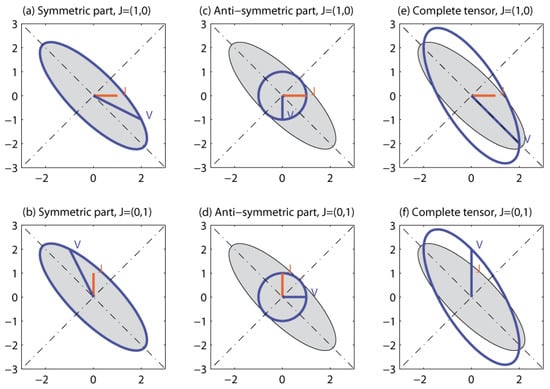
Figure 3.
(a–f). (a,b): Schematic illustration of symmetric behavior, illustrating the symmetric contribution for a given hydraulic gradient J (orange arrow). The resulting Darcy velocity vector V is shown as a solid blue arrow. Here, the principal system is at an angle θ = −π/4 with respect to the reference frame. (c,d): Schematic illustration of anti-symmetric behavior, illustrating the antisymmetric contribution for a given hydraulic gradient J (orange arrow). The Darcy velocity vector V is shown as a solid blue arrow. The orientation of the principal system (θ) plays no role in this antisymmetric component of the flow. The antisymmetric deflection is always orthogonal (90 degrees). (e,f): Schematic illustration of the complete behavior of an anti-symmetric and inclined permeability tensor K = KS + KA for a given hydraulic gradient J (orange arrow, visible in (e), but hidden behind V in (f)). The resulting Darcy velocity vector V is shown as a solid blue arrow. The principal system of the symmetric part KS is at an angle θ = −π/4 with respect to the reference frame. The antisymmetric part (KA) exerts an orthogonal deflection (always at 90 degrees), which does not depend on the θ angle.
In this example, the symmetric off-diagonal component is S = [KS]12 = −1, the antisymmetric part is A = 2, and the Frobenius norm is (see Equation (134) for the Frobenius norm). Thus, in this particular example, the symmetric and antisymmetric parts are of the same order of magnitude (as occurs also in some of our experiments on equivalent block permeability).
Table 1 and Figure 3a–f show two examples illustrating the relative effects of non-diagonality and antisymmetry on the Darcy velocity vector for a given hydraulic gradient vector . The main result shown in these figures is that the antisymmetric part (KA) exerts a systematic orthogonal deflection (always at 90 degrees) that adds up to the effect of the symmetric part (compare Figure 3c,d).

Table 1.
Antisymmetry effects on flow direction for a given hydraulic gradient vector J.
2.5. Boundary Conditions
Solving the equations of the local heterogeneous flow model and those of the upscaled macroscopic flow model requires in both cases to define a set of boundary conditions. In the following, we review the different conditions that are often considered and that we will use later.
2.5.1. Permeameter Boundary Conditions (PRM)
The permeameter boundary conditions correspond to the boundary conditions applied in the laboratory when measuring the hydraulic conductivity with a classical permeameter. They have been very often used to compute numerically the equivalent conductivity of heterogeneous media. The shape of the domain must include two parallel faces and correspond typically either to cylindrical cores or rectangular shaped samples. Based on this geometry, a constant head is prescribed on one of the two parallel faces and another constant head is prescribed on the opposite face, such that a global gradient is imposed in this direction. All the other faces are no-flow boundaries.
Note that, physically, laboratory samples are 3D (e.g., a cylindrical core, or a parallelepiped rectangle). However, quasi-2D samples can also be considered in the laboratory (thin slices, Hele-Shaw cells, etc.). To simplify our presentation, let us consider a two-dimensional experiment. We can express the permeameter conditions (PRM) as follows for a flow experiment with a head gradient imposed in the x1 direction:
L1 and L2 represent the dimension of the edges of the block, h0 the imposed head, the head difference between the two opposite faces, which are orthogonal to x1. In this “x1 flow experiment”, a head gradient is imposed in the x1 direction. The two other faces, orthogonal to x1, are no-flow boundaries.
2.5.2. Dual Permeameter Conditions (PRM’)
From a numerical point of view, it may be interesting to consider a novel configuration that generalizes the classical PRM permeametric conditions described above. Briefly, the new configuration consists of:
- two opposite faces with constant and identical non-zero fluxes, and
- linearly varying heads imposed on all other faces of the sample (instead of zero fluxes).
We propose to name these boundary conditions dual permeameter (PRM’) boundary conditions.
2.5.3. Constant Gradient Conditions (GRD) from Linearly Varying Boundary Heads
A constant gradient condition (GRD) is imposed by prescribing linearly varying heads along the boundary of the 2D domain or 3D domain, which may have complex geometric shape (usually convex). The linear form is defined in terms of a specified global or “far field” hydraulic gradient. This far field gradient occurs in the exterior of the porous domain and at its boundaries, hence the name “hydraulic immersion conditions” as if the porous sample were immersed in an ambient fluid characterized by a frozen macroscale gradient field. In the 3D case, for instance, this condition leads to a tri-linear macroscale head distribution on the boundary of the porous domain:
where J [-] is sometimes called “hydraulic gradient”; it is the opposite of the 3D head gradient vector (macroscale), and it can be expressed as:
With these notations, for any chosen orientation of the vector , the head distribution on the boundary is:
The same boundary conditions are applied on the microscale or macroscale experiments; therefore, we can use either the notation for micro or macroscale for the boundary conditions. In particular, for the case of a rectangular box-shaped domain, J1 is the total head drop between any points at location x2 = x3 = 0 taken on the two opposite faces orthogonal (⊥) to axis x1:
The linear head distribution (Equation (34)) can be applied on any domain geometry in a numerical model while they are much more difficult to apply in the laboratory, as opposed to permeameter type boundary conditions. Linearly varying heads were used by many authors, including [40,43,78,79,80,81]. For instance, the last authors [81] applied linear head immersion conditions or equivalently constant gradient conditions (named here GRD) to a sample of fractured porous medium.
2.5.4. Piecewise Gradient Conditions (GRD’)
As an alternative to the above GRD conditions, one may consider (and we will consider) piecewise constant gradient conditions (GRD’) implemented as piecewise linear head conditions on the boundary. The GRD’ conditions can be used to obtain analytically the local flow field on simple composite media (layered media, fractured media), and then perform averages to obtain explicitly an “exact” expression for the equivalent anisotropic conductivity tensor [80,82,83,84]. The last reference [84]), provides details in its Section 3.2.1 entitled “First step: equivalent permeability of unit blocks (upscaling single fracture/matrix blocks)”.
2.5.5. Constant Flux Immersion (FLX)
With permeameter boundary conditions (PRM), presented earlier, the flow is confined by impervious lateral boundaries around the sample. The flux immersion method (FLX) offers a more flexible manner to force the flow in any given direction, and this, for any domain shape. A constant macroscale vectorial flux is imposed by prescribing normal fluxes () on all elements of the boundary (on all points of the boundary Γ). Accordingly, let:
where is the unit normal vector defined on any point of the boundary Γ (outgoing normal). In addition, the head must be prescribed at a single point of the boundary to ensure unicity of the hydraulic head solution. These conditions can be understood as an immersion of the block in a frozen specific discharge vector field V (macroscale). This vector is projected normally on each boundary point and used as a boundary condition. These boundary conditions have been used, for example, by Pouya and colleagues [43,85] for fracture networks.
The flux immersion condition, as described here, is a dual version of the GRD conditions discussed earlier. Note: by the same token, piecewise flux conditions (FLX’) can also be constructed as an interesting analogy to the piecewise constant gradient conditions (GRD’).
2.5.6. Periodic Conditions (PRD)
Periodic conditions have been used widely used in the framework of homogenization theory [12,37,74]. They are applied on regular domain geometry (rectangle, hexahedron, etc.). In the case of a 2D rectangular domain, we can express them as:
where J1 and J2 are the components of the vector J. In addition, a value of the hydraulic head must be imposed on a single boundary point, otherwise the problem would have an infinite number of solutions. Note that in numerical codes, e.g., with discretized finite volume formulations and iterative matrix solvers, this may not be needed, as the initial guess can serve as forcing head condition (this is the case for example with the BigFlow 3D code, documented in [86]).
Note that periodic boundary conditions on a rectangular domain can be interpreted as a formulation of the flow problem on a torus (doughnut-shaped domain). This interpretation also implies a periodic pattern of all material properties involved: the internal geometry of the medium is repeated periodically (or equivalently, it is mapped onto the surface of a torus). Thus, for a fracture network, this would require a periodic distribution of all conductive objects (fractures). Similarly, for a multilayered medium, this would require a periodic distribution of all layers.
2.5.7. Skin Immersion (SKN) or Border Region
It is possible to prescribe the boundary conditions not directly on the boundary of the domain of interest, but further away, by considering that the domain of interest is immersed within a larger domain having the same kind of heterogeneity. This method was proposed by [87], and used later by several authors such as [55].
2.5.8. General Case with Mixed Head and Flux Conditions
More generally, the boundary Γ of the domain Ω may be divided into several parts, with various distributions of heads or fluxes on them. (Note: the term “flux” is sometimes used in this text to designate the specific discharge, or Darcy velocity vector.) For example, the boundary Γ can be separated into two parts, Γ = Γ1 ∪ Γ2, on which the head and flux are prescribed as given functions of space (respectively, and ):
3. Analytical Solutions of Darcian Flow Models
In this section, we present some analytical solutions of local-scale flow problems under specified boundary conditions in heterogeneous continua (these solutions are also applicable to macroscale problems with slowly evolving continuous permeability). In some cases, these analytical or quasi-analytical solutions have been backed up by numerical solutions obtained on fine grids (not detailed here). Such exact solutions can be useful for numerical benchmarks, and also for testing equivalent permeability criteria such as those studied in this paper. Note also that the equivalent permeabilities corresponding to other exact analytical solutions will be calculated explicitly for composite or layered media using our different equivalent permeability criteria (Section 5).
3.1. Velocity-Based Vectorial Flow Equation with Heterogeneous Permeability
This section is a more detailed continuation of the velocity-based flow equations that were briefly introduced in Section 2.2 on local flow models (Section 2.2.2: velocity based flow equations). We start with an introduction concerning the origins, motivations, and possible interest of such velocity-based flow equations before presenting it briefly.
It has been observed in the literature on Darcy flow that, for steady flow in a heterogeneous multidimensional medium, it is possible to use a system of PDE’s directly governing the Darcy velocity vector v (or the flux density q) taking into account both Darcy’s law and mass conservation without any explicit appearance of the pressure gradient or head gradient. This has several consequences:
- ✓
- The detailed Darcy velocity field resulting from the flux-based equations may be different from that obtained from the pressure-based equations. In theory they should be identical, but differences will arise due to the different approximations used either by perturbation methods or numerically in the flux-based and the pressure-based formulations; see for example Ababou ([68], Section 4.3 therein) and Akpoji et al. [72] concerning the flux vector variance in the case of a randomly heterogeneous spatially correlated medium (spectral perturbation solutions).
- ✓
- Using the flux vector equations, new flux solutions may be obtained potentially for various types of heterogeneous media, deterministic or random, either by analytical methods or numerically; in the case of a finite domain, boundary conditions on the flux vector must be considered, since the pressure gradient does not appear explicitly in the flux equations (as will be seen).
- ✓
- Another consequence of the flux-based approach is that it may lead to yet other definitions of the equivalent or effective permeability at the macroscale. Darcy’s law must still be used, but the averaging is performed on the detailed flux or Darcy velocity field resulting from the flux-based equation (not from the pressure-based equation). Just for this reason, the resulting macroscale may be different.
Briefly, the “flux-based”, or Darcy velocity-based flow PDE, is shown below for a multi-dimensional porous medium with spatially variable hydraulic conductivity :
where the symbol × denotes the vector product.
Let us also denote F(x) the log-permeability or log-conductivity field:
The term in parentheses in Equation (39) can be interpreted as the vorticity vector of the flow:
hence, the velocity-vorticity flow equation is:
A more advanced interpretation is developed in the aforementioned Appendices. For example, using indicial notations (with implicit summation on repeated indices), we have equivalently:
where is the strain rate tensor. Note that this equation is a second order vector PDE (a system of 3 s order PDE’s in 3D) governing the Darcy velocity vector (or “flux”) in a heterogeneous porous medium. It is somewhat analogous to a vector Poisson equation or Helmholtz equation. In the present case, for Darcy flow, it expresses that the vector Laplacian of velocity is driven by vorticity or by the divergence of strain rate. This velocity PDE could be solved, without using the hydraulic head field, under conditions of a prescribed Darcy velocity along the boundary of the domain.
To sum up: the previous formulation follows the vectorial velocity-based formulation of Darcy flow formulated in Ababou [68] for a heterogeneous continuum in general. For details with particular emphasis on the case of random filed log-permeability, Ababou [68], Section 4.3 therein: “New Closed Form Perturbative Solution for the Flux Spectrum”. This direct approach to velocity or flux solutions leads to stochastic analyses of flux variances, as in Akpoji, Ababou, De Smedt [70], based directly on the stochastic velocity equation. The velocity or flux-based equation was also presented in Zijl and Nawalany [69]; their Section 3.5 on “Directly calculated velocity components” (pp. 55–63) closely follows Ababou [68]′s work using different notations. We provide more details on the development of the velocity-based flow PDE in Appendix A.2: “Derivation of velocity-based PDE governing Darcy flow”, which is based on Ababou [68] (Section 4.3 therein).
3.2. Philip 1986 Analytical Flow Solution for a Continuous Periodic K(x,y) Pattern
In his paper, Philip [88] examines a special case of saturated flow in 2D periodic heterogeneous porous medium such that the flow can be described quasi-analytically by simple, periodic flow functions: the potential function and the stream function . The potential is associated with the hydraulic head and the stream function is associated with the streamlines of the Darcy velocity field . He also discusses an extension in 3D, but here, we will briefly describe the 2D periodic flow pattern. In Philip’s paper, the corresponding effective permeability is only mentioned in passing. Nevertheless, this particular flow field may be of interest for future equivalent permeability analysis.
Briefly, the 2D periodic permeability field treated by Philip [88] is of the form:
where is a reference value of permeability, obtained for instance at point , (and at all points located on horizontal lines ). In the remainder of this section, we take every where , or equivalently, the permeability is rescaled by taking . With this scaling, the permeability is bounded below and above by: .
The corresponding Darcy velocity field for this permeability pattern is given by:
The stream function was prescribed to be the following linear/periodic function:
Finally, the corresponding potential function can be determined by integration from:
Note that represents the local head gradient in our notations. Finally, note that, in fact, the permeability pattern of Equation (44) was inferred by Philip (1986) by solving exactly the following inverse problem: given the local flow pattern described by Equations (46) and (47), find the permeability field that satisfies this flow pattern: the result is the spatially distributed field given just above in Equation (44).
Figure 4 displays the permeability pattern and the corresponding flow field of Philip (1986) for .
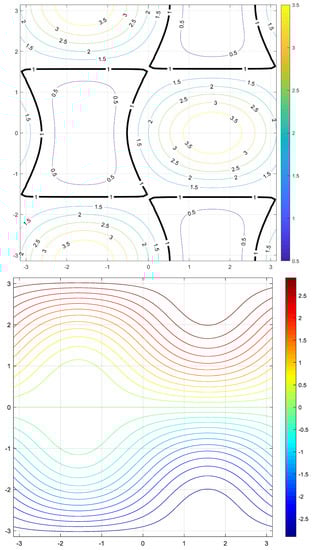
Figure 4.
Illustration of the 2D periodic flow problem of Philip [70] for , in a square domain . Top: Permeability contours . Bottom: streamlines obtained as iso-values of the stream function .
We now briefly consider an interpretation of the spatial pattern of as a probability distribution (due to Philip 1986), and possible extensions of this analysis to obtain the effective macroscale permeability from knowledge of , and .
- Firstly, Philip [88] states that, for his periodic permeability pattern, the effective “apparent” permeability (which he denotes “K*”) is by construction a scalar isotropic quantity equal to unity (K* = 1). However, no details are given concerning the definition of such an apparent permeability.
- Secondly, Philip [88] was able to re-interpret the spatial distribution of Equation (44) in terms of a probability density function of permeability (which he expresses in terms of an elliptic integral and plots in his Figure 3).
- We note that the (constant) effective permeability (possibly tensorial) could be computed according to various definitions and criteria to be presented later in this paper. This could be done in two different ways:
- by interpreting all local variables and coefficients in probabilistic terms (not only , but also , , and ), and then use probabilistic averages <…> to compute such that:
- Alternatively, the same objective could be achieved by replacing the probabilistic averaging brackets above <…> by spatial averaging brackets (being understood that the average is performed over a single periodic cell of the permeability pattern).
These suggestions have not been pushed further for the present periodic pattern; the probabilistic or spatial integrals needed are cumbersome, and it seems that the procedures suggested just above have not been carried out yet in the literature for this quasi-analytical flow pattern.
3.3. Analytical Velocity Field for Periodic Exponential-Cosine Permeability K(x,y,z)
The previous velocity-based equation (see also Appendix A.2) allows to obtain directly, in some cases, the Darcy velocity field for given permeability distributions, either exactly or approximately. We present below a velocity field in a finite domain with periodic permeability. This velocity is an approximation if one assumes a constant head gradient is imposed, but we will re-analyze it as an exact velocity solution with variable boundary head conditions on the finite size block. First, let us consider a 3D continuous porous block with a periodically variable permeability field (exponential-cosine function):
where is the spatial frequency or wave vector, is the amplitude of Ln(K) fluctuations, and is the geometric mean permeability. The following analytical velocity field satisfies exactly 3D steady state mass conservation , and it also satisfies Darcy’s law—albeit approximately (the approximation is first order in and it improves as decreases and becomes much less than unity).
Remark 1.
The above solution corresponds to a periodic medium with a single wave vector. It was used by one of us (R.A.) circa 1992 to test Lagrangian Particle Tracking algorithms on massively parallel Connection Machine. A more general Fourier expansion approximation based on spectral perturbation theory [32,68] was also developed for a broader spectrum of wave-vectors, and a similar general approximation was independently presented and used by Kapoor and Kitanidis [89] for illustrating solute dilution and concentration fluctuations in a heterogeneous aquifer (cf. their appendix: “Model Periodic Hydraulic Conductivity and Flow Field”, p. 313 therein).
Figure 5a shows a plot of the 2D periodic exponential-cosine permeability field:
with .
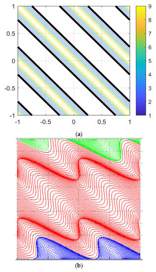
Figure 5.
(a,b) Analytic Darcy flow problem with exponential-cosine permeability: permeability field, streamlines, and hydraulic head field, from top to bottom. (a): contours of the periodic permeability field with ; the bold black contours correspond to geometric mean permeability ; the broad white zones without contour lines correspond to the relatively flat minima of . (b): streamlines of the analytical Darcy velocity field given in the text.
Figure 5b shows a plot of this 2D periodic permeability field, and of the streamlines corresponding to the 2D analytical Darcy velocity field with the above parameters and .
Before proceeding further, let us note that the previous velocity field solution was inspired by spectral perturbation solutions of Darcy flow in an infinite domain with randomly heterogeneous permeability (the periodic permeability proposed here represents only a single non-random Fourier mode from the spectral perturbation approach). The resulting periodic velocity field above (Equation (49)) is only an approximation of the local velocity if one assumes that the flow domain is infinite and that the flow is submitted to a constant large scale hydraulic gradient: in that case, the velocity of Equation (49) satisfies exactly mass conservation but only approximately Darcy’s law.
However, let us now take a different viewpoint in two ways: (i) by restricting the flow problem to a finite domain (e.g., 2D square or rectangular domain), and (ii) by seeking boundary conditions such that the local velocity field given above of Equation (49) becomes exact. This is achieved by the following “inverse” procedure, that is, inverting Darcy’s law as follows:
where is the local hydraulic gradient defined by , and is the periodic “exponential-cosine” function of space, defined earlier.
Note that the flow field defined by , , and now satisfies exactly both mass conservation and Darcy’s law with the specified exponential-cosine permeability field .
It is now possible to explicitly obtain the head distribution inside the square domain, and along its boundary as well (four faces: left, right, bottom, top). To obtain at any interior or boundary point , one may first integrate horizontally the horizontal gradient component and then vertically the vertical gradient component , following for instance the integration path illustrated in the schematic of Figure 6.
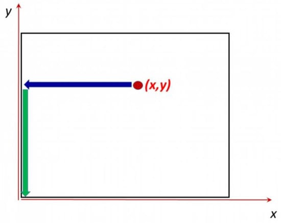
Figure 6.
Schematic representation of an integration path to obtain the head at any point , given the hydraulic gradient field .
Assuming for convenience a rectangular domain , the quasi-analytical result is:
where the vector is known analytically from the previous inverse Darcy relation. The simple integrals were carried out with a simple histogram method (mimicking Rieman integral), and the resulting head distribution inside the domain is displayed in Figure 7 for the same case of highly variable periodic with as in the previous figures.
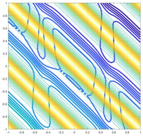
Figure 7.
Quasi-analytical hydraulic head field given in the text, shown as bold contours. The contours of periodic permeability with are also superimposed as thin curves. The broad white bands of correspond to zones of minimal permeability, coinciding also with zones of large head gradient.
Remark 2.
, the standard deviation of LnK(x,y), plays the role of an amplitude parameter here; the heterogeneous domain is very variable for and, on the contrary, it becomes nearly homogeneous for .
Finally, from the previous head solution , which is valid both at interior points and at boundary points, we now deduce the four head profiles along the four boundary faces of the domain, as follows Equations (53)–(56):
The corresponding profiles of boundary heads are plotted in various ways, for the high variability case (), in Figure 8. We have taken the head value at the lower left corner to be zero: . Reminder: in all such figures (velocities, streamlines, heads), the domain is a square with coordinates and , and therefore, the domain size is .
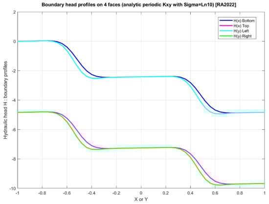
Figure 8.
Plot of the 4 profiles of hydraulic head or along the 4 boundary faces of the square domain with periodic “exponential-cosine” permeability for (high variability). It can be seen that the continuity of hydraulic head at the 4 corners of the square domain is ensured (more on this in the text).
Note in particular that the continuity of hydraulic head at the four corner nodes is satisfied; for instance, at the bottom right corner , the head value from the bottom horizontal profile at is the same as the head value from the right vertical profile at . They can be seen to be identical graphically from the plotted boundary profiles of Figure 8. We have verified indeed that head continuity is ensured with relative precision better than 1/1000, and it is also continuous analytically. The unique value of head at the bottom right corner is numerically , and analytically:
Furthermore, due to the periodic permeability field, the head field has a number of symmetries, as can be seen from in Figure 7, and from the boundary head profiles of Figure 8. Thus, in Figure 8, the bottom profile in dark blue is nearly identical to the left profile in cyan color. Similarly, the top profile in magenta is nearly identical to the right profile in green. The slight discrepancies between the bottom/left profiles and between the top/right profiles are only due to coarse numerical integration (the graphics shown here use a discretization of the domain into 50 × 50 pixels or 51 × 51 nodes; these discrepancies will vanish for finer numerical integration grids).
In summary, an exact quasi-analytical finite domain flow under prescribed spatially variable head conditions was presented in this subsection for a periodic permeability field. The sample appears to be stratified with an angle of stratification of 45 degrees (in our example). This sample flow problem could be further exploited to infer the equivalent homogeneous permeability using one or several of the methods or criteria that will be presented later in this paper.
4. Equivalent Conductivity: The Criteria
Definition 1.
The equivalent block conductivity K is the hydraulic conductivity of a fictitious upscaled homogeneous medium such that certain average quantities (the equivalence criteria) are equal if we compute them both on the real heterogeneous medium and on the upscaled medium when the same boundary conditions are imposed on the two media. NB: more precisely, in some methods it is the equivalent conductivity matrix that is obtained; in other methods the resulting conductivity K can be shown to be a true second rank tensor .
To apply the previous definition, the equivalence criteria must be defined precisely. In the next paragraphs, we describe the average quantities that have been used to define the equivalence between the heterogeneous and upscaled media. In each case, we distinguish (when necessary) between the three types of heterogeneous media defined earlier: (1) continuous, (2) composite, and (3) fracture networks. In the case of fracture networks, hydraulic conductivities vanish in most of the domain except in the fracture set, and for this reason, the permeable domain is partially disconnected, and so is its boundary Γ. Due to this extreme type of discontinuity, we use special dedicated formulations for flux averages and equivalent conductivities. In all cases, the previous formal definition requires the computation of the equivalence criteria both on the heterogeneous and on the homogeneous media.
4.1. Average Quantities and Equivalence Criteria
In this section, we present several criteria (for instance based on different kinds of averages of flux and hydraulic gradient, or total dissipated power, etc.) that can be used to define the equivalent block-scale permeability. For each type of criterion, the case of a porous continuum sample is treated in detail, and in most cases, the same expressions hold also for a composite porous sample (in addition, the corresponding expressions for the special case of a block consisting of a 2D fracture network are summarized).
4.1.1. Net Surface Flux (NSF)
The Net Surface Flux (NSF) criterion is the first and most obvious criterion that was used [90,91]. It is based on the analogy with the permeameter experiment.
The idea is that the net fluxes through the surfaces of the heterogeneous and homogeneous media must be identical. It is perfect for isotropic medium. However, it leads to some difficulties for anisotropic medium; when all the faces of the domain are open to flow, the flux entering the domain through a given face can be different from the flux leaving the domain through the opposite face. A way to circumvent this issue is to use an average: the mean between the fluxes on the two opposite faces (in the case of rectangular geometry).
NSF Criterion for a 2D Rectangular Porous Sample
Thus, for a 2D rectangular porous sample, the x1 component of the net surface flux vector is then defined by the following expression for continuous and composite porous media:
where the minus sign results from the opposite orientation of the normal vectors () for two opposite faces in rectangular geometry (in this paper, the normals are outgoing, see Figure 1).
NSF Criterion for a 2D or 3D Porous Sample of Arbitrary Shape
For the sake of generality, we propose a set of expressions that can be used on any geometry of the porous sample in two or three dimensions. For that purpose, we assume that only surface fluxes at the boundary of the domain are available to measurements and not vectors. Under these constraints, we derive (see Appendix A.4) the following set of equations in two dimensions.
where , , and are three scalars that depend only on the geometry of the domain and on the coordinate system, and and are two oriented and integrated surface fluxes, as follows:
In these equations, ui is the unit vector along direction i. In the special case of a rectangular domain, Fi boils down to the total flux normal to the face orthogonal to ui. This set of equations leads to Equation (57) when the domain has a rectangular shape. The formula is consistent, that is, when applied to a constant velocity field within the domain it yields the components of this constant velocity vector (as it should). The general expressions for the 3D case are given in Appendix A.5.
NSF Criterion for a 2D Fracture Network
Although we have not systematically specialized our analyses to fracture networks in this paper, it may be useful to consider the previous “NSF” criterion when applied to a 2D fracture network consisting of an impervious block traversed by thin fractures (segments in 2D). For such a fracture network, NSF expressions similar to the previous ones can be obtained via a discrete summation of the fluxes at the boundary of the fractured block.
To illustrate the principle of this summation, Figure 9 shows a simple square block. On the external boundary of the block, only the incoming or outcoming fluxes are assumed to be measurable. These quantities are defined for each node i located on the boundary and denoted . By convention, is positive if the flux enters the block and negative if the flux exists the block. With this notation, the horizontal component of the Net Surface Flux can be expressed as the average flux between the two opposite faces (see Appendix A.4 for a generalization).
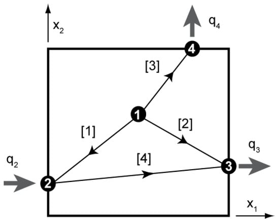
Figure 9.
Schematic illustration of the NSF criterion on a simple fracture network. Note that only the normal fluxes perpendicular to the faces of the block are available at the nodes that are located on the boundary (compare to the VSF method of Figure 10).
Using either Darcy’s law or Poiseuille’s law, it is possible to express the vectorial fluxes at all boundary nodes of the fracture network. One can then express formally the Net Surface Flux by multiplying the fluxes by a matrix having two lines (for two vector components in 2D) and as many columns as the number of boundary nodes. The coefficients of this matrix are computed in order to project the fluxes on the right direction, and we obtain the mean NSF velocity as follows in terms of border fluxes
Conclusions on the NSF Criterion
Even if the Net Surface Flux (NSF) criterion has some interesting features, such as its consistency, it does not allow capturing properly the deviation of flow that can occur in a medium. For example, if the flux enters a face at the base of the face and leaves the opposite face near a corner, it is clear that there exists a diagonal component in the flux that we cannot capture with the NSF. This is why other formulas are required; this is the motivation for the formulas described in the next sections.
4.1.2. Vectorial Surface Flux (VSF)
In some situations, it is possible to directly access the vectorial fluxes at the boundary of the domain. For example, the flux vectors (or velocity vectors) can be accessed quite directly at the boundary of a fractured block consisting of a 2D fracture network, but more generally, they can also be computed on the boundary of any continuous or composite porous block.
VSF Criterion for a Porous Sample in 2D or 3D
It is quite natural to define an average vectorial surface flux at the boundary of the sample by simply averaging all those vectors. This can be done by a surface integral as follows, for a sample of continuous or composite porous medium (generally in three-dimensional space).
VSF Criterion for a 2D Fracture Network
In the case of a 2D fracture network, one can use instead a discrete summation over all the individual fractures hitting the boundary of the block, as shown for illustration in the example of Figure 10:
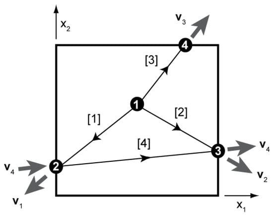
Figure 10.
Schematic illustration of the VSF criterion on a simple fracture network. Note that the directions of the fluxes are also available (contrary to the NSF method of Figure 9). In this case, the vectors are summed over all the edges touching the border.
4.1.3. Volume Averaged Flux (VAF)
Another interesting alternative technique to get a mean vectorial flux in the block is to average the Darcy velocities over the whole domain of interest as proposed by [92]. This is what we define as the Volume Average Flux
This concept can be less intuitive than the two previous averaging methods (NSF and VSF) when one thinks about a laboratory experiment in which the Darcy velocities inside the block are not easily accessible. Of course, this is not an issue for numerical experimentation. However, this is also not a problem in a laboratory experiment because the volume averages can be replaced by surface integrals [93] as shown in Appendix A.7:
Developing the previous equation on square geometries leads to an average of the total surface fluxes weighted by the coordinates of the centers of gravity of those fluxes on the different faces (Appendix A.7.3 and Table 2). Note that these equations have been used to construct a prototype of tensorial permeameter in the laboratory [25].
Table 2.
Equivalent permeability criteria: specialization of volume averages to surface averages for specific boundary conditions and block geometries (see Appendix A.7 for proofs).
VAF Criterion for a 2D Fracture Network
On the example of the previous fracture network (see also Figure 2), applying the VAF criterion in a discrete manner yields (for a square domain):
4.1.4. Volume Averaged Gradient (VAG)
Up to this point, we only discussed average quantities related to the Darcy velocities. However, depending on the boundary conditions, it may be necessary as well to estimate an average hydraulic gradient.
For example, when imposing permeameter type boundary conditions, only the head gradient in one direction is imposed during a single experiment, but the perpendicular gradient components also need to be computed.
As another example, when imposing a fixed constant vectorial flux to the boundaries of the domain, these fixed velocities are interpreted as the block scale velocities, and only the average head gradient requires to be computed as a function of the heterogeneity.
In all those situations, the average gradient is computed as the volume integral over the local gradients within the domain, as proposed by Rubin and Gómez-Hernández [92].
Like for the Volume Average Flux, one can transform the volume integral into a surface integral [93] to facilitate its computation or its measurement in a real experiment (see Table 2 and Appendix A.7.2).
Among the results concerning this quantity, it is important to note that the volume average gradient is equal to the far field gradient imposed through linearly varying head boundary conditions for any geometry, and it is also true for periodic boundary conditions. This result is true both for the heterogeneous and homogeneous media because it depends only on the head distribution along the boundary.
In conclusion, the Volume Average Gradient (VAG) is identical to the opposite of the macroscale hydraulic gradient vector, which serves to impose linearly varying head conditions on the boundary of the domain. That is, we have:
where is the hydraulic gradient vector in the linearly varying head boundary conditions:
A similar linear distribution of hydraulic heads can be expressed at the boundary of a fracture network, by prescribing at all fracture boundary points. These are the intersection points of fractures with the immaterial boundary of the computational domain (e.g., a rectangular block).
4.1.5. Total Dissipated Power (TDP)
The last very important physical quantity that we will consider in this paper is the Total Dissipated Power. This quantity was frequently used to define the equivalent hydraulic conductivity [30,94,95,96].
When flow occurs through a porous or fractured medium, a dissipation of energy occurs, which corresponds to the hydraulic head loss along the flow field. This energy loss is equivalent to the work of the viscous forces that resist the flow.
TDP for a Porous Continuum
In the case of a porous continuum, the total energy dissipated per unit time within the porous domain is the total dissipated power P [Watt] defined as
where g is the acceleration of gravity [m/s2] and ρ is the mass density [kg/m3] of the fluid.
TDP for a Fracture Network
Briefly, for a 2D fracture network, the equivalent expression of the Total Dissipated Power P is of the form:
where the summation is over all conductive arcs, or fracture segments, in the network.
4.2. Defining the Equivalent Conductivity Tensors
In this section, we describe how the equivalent block conductivity tensor (or at least the equivalent conductivity matrix) can be expressed and calculated, depending on the choice of the equivalence criteria and of the boundary conditions imposed on the sample block. We treat generally the case of continuous or possibly composite porous samples, and we also briefly provide the corresponding expressions for the special case of a 2D fractured block consisting of a network of fracture segments. We end up with a special consideration of the dual matching procedure for determining the equivalent permeability and resistivity, which, although not implemented numerically in this paper for the various block scale samples of Section 6, has proven useful in the context of upscaling for randomly heterogeneous media via analytical perturbation methods (e.g., [75]).
4.2.1. Equivalent K from Permeametric Experiment: Diagonal K Matrix (DIAG)
Since the first numerical studies of the equivalent permeability of heterogeneous media [91], the equivalent permeability “K” is often estimated by imposing permeameter type boundary conditions and computing the net surface flux through the heterogeneous medium in the direction of the imposed gradient. Assuming that the main axes of anisotropy of the medium are parallel to the axes of the sample, the net surface flux through the homogeneous medium is simply equal to the imposed head gradient times the diagonal element of the equivalent conductivity tensor corresponding to the direction of the flow experiment.
Consequently, one can estimate the equivalent (diagonal) conductivity matrix in the coordinate system of the porous sample, provided three numerical simulations (in 3D) or two numerical simulations (in 2D). Taking the 2D example yields the following diagonal K matrix (note: it is not the equivalent conductivity “tensor” that is “diagonal”; rather, it is the equivalent conductivity matrix K that is diagonal in the coordinate system of the block.):
In that expression, is the net surface flux in the x1 direction computed from the first numerical experiment (hence the superscript 1) with a gradient imposed in the x1 direction. Similarly, is computed from the numerical experiment in the perpendicular direction.
The same expression can be written in 3D; it only requires running an additional flow experiment in the x3 direction.
In the following, the DIAG method correspond to the results obtained with Equation (74) whether they are computed from experiments made using permeameter type or linearly varying head boundary conditions. In other words, the DIAG method consists of using the NSF criterion and neglecting the off-diagonal components of the equivalent permeability matrix expressed in the coordinate system of the porous sample. This method is obviously not adequate for identifying the full permeability tensor in the general anisotropic case, but is used here to allow a comparison with the other techniques that are presented below.
Note: “matrix” and “tensor” should be distinguished. Indeed, assuming that the equivalent K is a second rank tensor (), then the permeability matrix K (diagonal or not) is merely the representation of this tensor in the reference system (in the present case, for permeametric conditions, the reference system is aligned with the porous block sample).
4.2.2. K from Net Surface Flux (NSF)
A natural extension of the previous definition (DIAG) to anisotropic media is to consider the Net Surface Flux (NSF) to define an equivalent conductivity. Using this criterion, KNSF is defined such that the net surface fluxes are identical in the heterogeneous and homogeneous media.
The brackets represent the averaging operator described in Equations (57)–(62) for the 2D case, and in Appendix A.5 for the 3D case. Recall that lower case represents local microscale velocity (which can be highly variable in space), while upper case represents macroscale velocity (which can be either constant or mildly variable in space). Caution is required with the <…>NSF averaging operator because it involves an integration of the normal fluxes on the boundary of the sample.
It is possible to express KNSF from Equation (75) after some manipulations. However, this leads to a complex averaging operator for the head gradient along the boundary of the domain. In fact, the problem lies not in this complex integration but in the fact that the spatial distribution of the head gradient along the boundary of the sample is itself a function of KNSF. This means that in the general situation, one cannot manipulate Equation (75) to provide a closed form expression of KNSF without making an additional assumption.
When the hydraulic gradient J = −∇H is constant along the boundary of the domain of the homogenized porous block, Equation (75) has a closed form solution. This situation occurs, for example, when imposing linearly varying head, a constant vectorial flux, or periodic boundary conditions. When this is the case, the NSF formulas have been derived to ensure consistency, and we have under these conditions. We then obtain the following operational definition of the equivalent conductivity tensor from the NSF criterion with GRD, FLX, or PRD boundary conditions:
When the head gradient is not constant in the homogeneous domain, one can use an estimation of the mean gradient within the domain and along the boundary to find an approximate solution to Equation (75). We propose, then, to use the volume average gradient criteria (VAG). This leads to the following operational definition for KNSF.
Note that this last equation is identical to Equation (76) when using GRD, FLX, or PRD boundary conditions since the Volume Average Gradient in these cases is equal to the imposed gradient −J. In the numerical experiments that will be described in Section 6, we will apply Equation (77) in all cases, that is, also in cases where the boundary conditions are not imposing a constant gradient in the homogeneous domain (PRM, for example), and we will illustrate numerically that the computation of KNSF using Equation (77) does not always ensure the equality Equation (75).
Like for the DIAG method, two numerical experiments are necessary to identify all the components of KNSF in 2D (or three experiments in 3D). Equation (77) is written for each numerical experiment and assembled in a linear system where the unknown is the hydraulic conductivity tensor KNSF. This yields:
where stands for , and the superscript 1 or 2 associated with an average quantity is used to identify the flow experiment. The above equation can also be written in matrix notation:
In this equation, is a square matrix, whose columns contain the volume average gradient components computed for a given numerical experiment; VNSF is a square matrix as well, containing the corresponding Darcy velocities organized in a similar structure. The matrix representation is identical in 2D and 3D. If is invertible, the solution is obtained by multiplying both sides of the equation by :
In 2D, this explicit solution for the NSF equivalent permeability is simply:
with: .
Note that Equation (81) contains all the components of the head gradient vectors for both numerical experiments. This allows computing the off-diagonal terms of the equivalent conductivity matrix . A similar procedure was employed by Kfoury et al. (2006).
To ensure that is invertible, it is convenient to select the boundary conditions of the 2 in 2D or 3 in 3D numerical experiments such that the directions of the gradient are perpendicular. In particular, when constant gradient (GRD) or periodic conditions (PRD) are used, it is very convenient to use unit gradients aligned with the coordinates systems ( for i = 1, …, 3), then becomes the identity matrix ( = −I) and the previous equations become simply, under these unit gradient conditions:
As already explained earlier, the previous Equation (77) and all its simplifications just above ensure the equality of the NSF criterion between the homogeneous (homogenized) medium and the heterogeneous medium, when using either GRD or PRD boundary conditions (head gradient or permeametric conditions). However, Equation (77) remains an approximation in the general case.
Equivalent K with the NSF Criterion for a 2D Fracture Network (Summary)
Briefly, in the case of a 2D fracture network, and for constant head gradient conditions (GRD), we have found that the equivalent permeability resulting from the previous NSF criterion can be expressed as:
In this expression (Equation (83)), represents the resulting equivalent conductivity tensor (see comment on this further below). The other quantities are defined as follows:
- ▪
- Quantities such as designate node–node Laplacian matrices, weighted by the conductances C of the fracture segments (links) relating the nodes (intersections). The discrete Laplacian matrix corresponds to the continuum Laplacian operator but with discrete versions of the and operators (they are expressed on the graph representing the fracture network). The conductivities are replaced by conductances C based on either Darcy or Poiseuille’s law for flow through each link. The Laplacian matrix to be inverted in Equation (83) is the internal node–node matrix of size . Other auxiliary node–node Laplacian matrices appear also; they are indexed depending on whether they concern internal nodes (I) and/or boundary nodes (F): thus, is the Laplacian matrix of size relating all internal nodes, while of size is the Laplacian matrix relating internal nodes to boundary nodes, and of size is the Laplacian relating all boundary nodes between them (if there does not exist a single link between any pair of boundary nodes, then ).
- ▪
- represents a geometric matrix of size containing the two components of the unit vector normal to the block at the NF boundary nodes (which are submitted to linearly varying head for the present case of gradient condition “GRD”);
- ▪
- represents a coordinate matrix of size with lines (number of boundary nodes) and two-columns containing the coordinates of the boundary nodes;
- ▪
- L is a scalar representing the size of the 2D fractured domain (here a square block); note: the domain size “L” should not be confused with the Laplacian matrix “L”.
With these definitions, the reader can check that the resulting equivalent conductivity is indeed an indexed matrix ; furthermore, analyzing the algebraic nature of the expression of Equation (83), it can be shown that the resulting behaves like a second rank tensor. Properties of this equivalent tensor, and those obtained by applying other criteria, have been analyzed by us [61,62]) and will be presented in more detail elsewhere in future (e.g., [97]).
For more details on the algebra of graphs, see Gil Strang’s seminal paper on equilibrium problems in hydraulics and structural mechanics [98], where graph structures and algebraic approaches are emphasized. His ideas were also presented more recently in a book ([99], Chap. 2: A framework for applied mathematics therein).
4.2.3. K from Vectorial Surface Flux (VSF)
In a similar manner, we can define the equivalent conductivity tensor KVSF such that the Vectorial Surface Flux is identical on both the homogeneous and heterogeneous media. Here, the averaging operator is simpler than for the VSF expression and can be expressed as surface integrals on the local and homogenized Darcy velocities (i.e., the microscale and macroscale velocities).
Replacing the large-scale specific discharge V by the upscaled Darcy’s law with a constant tensor leads to the following definition of the equivalent conductivity for continuous or composite media:
Like for the NSF method, the average value of the gradient on the frontier of the block of the homogeneous medium is not known in general as it is a function of , the geometry of the block, and the boundary conditions. If the boundary conditions are such that the gradient is constant in the homogeneous medium, then this average quantity is known and independent from the value of . It is equal to the imposed gradient. If this is not the case, we use the volume average gradient on the heterogeneous medium as a reasonable approximation.
To compute , Equation (86) is used twice in 2D or three times in 3D with different numerical experiments in order to identify all the components of the conductivity tensor with an expression analogous to Equation (80).
The only difference with Equation (80) is that the averaging technique used to compute the mean velocity is here the Vectorial Surface Flux while it was the Net Surface Flux in the previous method. Again, if linearly varying head or periodic boundary conditions with unit gradients aligned with the system of coordinates, one can use a similar expression as Equation (82) with the VSF averages.
Equivalent K with the VSF Criterion for a 2D Fracture Network (Summary)
Briefly, in the case of a 2D fracture network, and for constant head gradient conditions (GRD), we have found that the equivalent permeability resulting from the previous NSF criterion can be expressed as:
where (briefly): is a matrix indicating the direction vectors of the “boundary” fracture links that intersect the boundary of the domain; and are submatrices that relate (through conductances) those links to (respectively) the boundary nodes () and the interior nodes (I); is the square Laplacian matrix of size over all interior nodes; is the Laplacian matrix relating interior to boundary nodes; and is an coordinate matrix containing the two coordinates of the boundary nodes. Note that matrices are of the form , where is the diagonal conductance matrix and is the node–node adjacency matrix. The resulting equivalent permeability is given explicitly by Equation (88), in an algebraic fashion. The main computational task is (as before) the inversion of the square Laplacian matrix .
4.2.4. Volume Average Flux (VAF)
A third possibility is to define the equivalent conductivity tensor KVAF such that the Volume Average Flux (VAF) is identical on both the homogeneous and heterogeneous media. Here, the averaging operator is a volume integral, although we have already seen that it can be replaced by a surface integral without any loss of generality. The volume average flux criterion is:
Replacing the macroscale Darcy velocity V by the upscaled Darcy’s law leads to the following definition of the upscaled VAF conductivity :
As before, is implicitly in the volume integral because H is a function of the geometry of the block, the boundary conditions, and . When constant gradients (GRD) or periodic boundary (PRD) conditions are used, then the Darcy velocity and the head gradient are constant in the domain, whatever is its geometry, and the volume average gradient is directly known. In the other cases, we will invoke an additional criterion, which is that the volume averaged head gradients in both the heterogeneous and homogeneous domains should be equal:
Using both the VAF and VAG criteria leads to the operational definition of the equivalent conductivity used by many authors since Rubin and Gomez-Hernandez (1990):
Here, it is important to note that the reciprocal may not be true, computing from Equation (92) does not necessarily imply that the VAF and VAG criteria are both verified.
As for KVSF or KNSF, KVAF is computed numerically by solving two numerical problems in 2D or three in 3D and by applying Equation (92) for each numerical experiment. All those equations are assembled to identify all the components of the conductivity tensor.
with and being the matrices containing the compilation of the volume average fluxes and gradients computed from the results of two numerical experiments with perpendicular gradients as explained in detail earlier (see Equations (78) and (81)).
As before, this equation can be simplified for linearly varying head or periodic conditions with unit gradients.
Equivalent K with the VAF Criterion for a 2D Fracture Network (Summary)
Briefly, in the case of a 2D fracture network, and for constant head gradient conditions (GRD), the equivalent permeability resulting from the VAF criterion is of the form:
where the various matrices are defined as in Equation (83), with Laplacian matrices (boundary nodes to boundary nodes), (interior nodes to boundary nodes), (interior nodes to interior nodes), and is the rectangular matrix of coordinate positions of the boundary nodes. Again, the 2D block is assumed here to be a square of side “” (not to be confused with a Laplacian matrix).
4.2.5. Equivalent K with the Volume Average Gradient (VAG) Criterion
We have seen that in the previous definitions of the equivalent conductivity, we often had to use the volume average gradient as complementary information. In addition, when constant flux boundary conditions are used, all the previous criteria are directly imposed by the boundary conditions and cannot be used to define K. In this case, one has to use the Volume Average Gradient to define and compute the equivalent conductivity .
Using the large-scale Darcy’s law, and taking out of the averaging operator, one obtains:
Like for the previous cases, one can fully identify by running three different flow experiments. When using constant flux (FLX) boundary conditions, the right-hand side of Equation (97) is imposed by the boundary conditions. If we assume that the two numerical experiments are designed with unit vectorial fluxes oriented along the and directions, we get the following expression for .
4.2.6. Equivalent K from the Total Dissipated Power (TDP) Criterion
Some authors such as [30,94,96,100,101] used the Total Dissipated Power to define the equivalent hydraulic conductivity. As in the previous definitions, the principle here is to state that the total dissipated power must be identical in the heterogeneous medium and in the corresponding homogeneous (homogenized) medium:
If we replace, in the right-hand side, the block scale or macroscale V by the macroscale Darcy phenomenological law, we then obtain the following definition of the equivalent conductivity matrix :
This criterion has been used very successfully for deriving bounds for the equivalent conductivity [43,94]. However, because this criterion leads to a scalar equation, it is a priori less convenient than a vectorial criterion if the objective is to calculate a non-diagonal equivalent conductivity matrix (or more generally, the equivalent conductivity tensor). In particular, because each numerical experiment will provide only one equation, this criterion (Equation (100)) will require running more flow simulations than the other techniques.
To avoid that problem, Bøe [96] proposes to split the implicit sums resulting from the product of the head gradient with all the components of the Darcy velocity in the criterion of Equation (100). This results in a set of nine sufficient criteria involving a basis of three numerical flow problems in perpendicular directions whose solutions are h1 to h3. Assuming that the boundary conditions are periodic, Bøe [96] proposes an operational definition, which can be written with our own notations as follows.
This expression (Equation (101)) is a sufficient condition to satisfy the TDP criterion. It was also suggested by Farmer [35] as “a natural” definition of the equivalent conductivity without stating a specific equivalence criterion. Both Bøe [96], assuming a diagonal local conductivity tensor and periodic boundary conditions, and Farmer [35], for a symmetric but not necessarily diagonal local conductivity tensor and linearly varying head, show that the previous equation can be written in a more complex form.
Equation (102) is not used to compute , but it directly shows the symmetry of obtained from Equation (101) if one uses linearly varying head or periodic boundary conditions. If the intensity of the gradient is Ji = 1 in each numerical experiment, Equation (101) is identical to Equation (94). Furthermore, the resulting tensor is strictly the same as the one computed by the VAF technique when using GRD or PRD boundary conditions. Therefore, in the remainder of this paper, we will not consider that approach as a distinct approach to compute K. Instead, because the TDP is an important criterion, we will test whether all the other definitions of the equivalent conductivity tensor will satisfy the total dissipated power.
4.3. Dual Permeability/Resistivity Matching
We end up with a brief presentation of the dual permeability/resistivity matching procedure for determining both the equivalent permeability and equivalent resistivity. This procedure will not be implemented numerically to the various block samples studied in Section 6 (some of them random, others deterministic), but it is worth mentioning, as it has proven useful in the context of upscaling flow in randomly heterogeneous media via analytical perturbation methods (e.g., [75,102,103]).
This approach is based on the local head governing PDE , but uses it in two different ways to obtain an upscaled Darcy law (two “dual” approaches):
- upscaling is performed in terms of the local hydraulic conductivity k (based on Darcy’s law v = −k(x).∇h), leading to an equivalent macroscale conductivity K, and…
- upscaling is also conducted in terms of hydraulic resistivity r = k−1 (based on the reciprocal formulation of Darcy’s law −∇h = r(x).v), leading to an equivalent macroscale resistivity R.
The term “conjugate” or “dual” was introduced in Ababou ([1], Chap.4) to describe the particular invariance properties of 2D heterogeneous continua with equilibrated distributions, under the transformation →, exploiting and generalizing previous results by Shvidler [73] and Matheron [30]. The term “dual upscaling” was later applied to the tensorial macro-resistivity Rij obtained by upscaling −∇h = r(x).v in any number of spatial dimensions, where r(x) is the local resistivity (e.g., [102] for single phase flow in a 3D random medium). This “dual” approach leads to a comparison of Kij and Rij based on algebraic positivity and reciprocity upscaling criteria: [Rij] > 0; [Kij] > 0; [Rij] = [Kij]−1.
These criteria were presented in Fadili and Ababou [75] for a random continuum with spatially correlated log-parameters, first for single phase flow, and secondly for immiscible two-phase flow based on Darcy–Muskat equations, with nonlinear retention curves and two-phase permeability curves. This permeability/resistivity approach had also been presented earlier, for single-phase Darcy flow in randomly heterogeneous media (e.g., [102,103]). In summary, the main result for the case of a statistical Darcian continuum with random field Gaussian log-conductivity is of the form:
See also around Equation (101) in Appendix A.8. This formulation achieves several desirable properties: (i) it is thought to ensure the robustness of the small parameter approximation thanks to the exponential extrapolation; (ii) it satisfies both the reciprocity relation and the positivity criterion for permeability and resistivity; and (iii) it preserves the tensorial nature of effective permeability and resistivity (for more details, see Appendix A.8). The permeability/resistivity matching approach could be considered in the future for application to finite domain upscaling, that is, matching macroscale block-permeability and block-resistivity.
5. Explicit Expressions of Equivalent Conductivity Tensors for Layered Media
In this section, we develop expressions of equivalent conductivity tensors for a few special types of heterogeneous media or fracture networks with prescribed boundary conditions.
This section shows that piecewise linear head conditions lead (analytically) to a tensorial Kij. Two methods were developed, one by Renard ([80], Annex B therein), and the other was presented by Cañamón et al. [82,83] and Ababou et al. [84]. These methods yield the same types of results for slightly different layered configurations. In the latter method, the microscale velocity and head gradient fields are piecewise constant, and the microscale head field is piecewise linear, both on the boundary and inside the layered domain. Furthermore, the microscale and macroscale head fields (h and H) do not obey the same boundary conditions, unlike the gradient condition “GRD” with linearly varying head condition, presented in Section 2.4. The present approach with piecewise linear head conditions can be described as follows:
- Conditions: immersion in a piecewise constant gradient (GRD’) or flux (FLX’)
- Criteria: Volume Average Gradient and Volume Average Flux (VAG+VAF)
5.1. Exact Flow Solution and Equivalent Permeability for a Three-Layered Fractured Medium under Piecewise Linear Head Conditions (GRD’)
We present here a special analysis that produces an exact tensorial Kij for multi-layered 2D or 3D prismatic domains submitted to specific piecewise linear head distributions on the boundary (GRD’). Among the various upscaling methods analyzed in this paper, these particular head boundary conditions were not fully investigated in the previous section; however, this case is still relevant because the simple flow solution obtained with these conditions on a layered block leads to an exact evaluation of the equivalent block permeability tensor Kij, which can be used as a reference for comparisons with other methods. Cañamón [82], Cañamón et al. [83,104]), Ababou et al. [61], applied the method to a composite matrix/fracture “unit block”, as the first step in a sequential upscaling procedure for 3D fractured porous media with a permeable isotropic matrix. The fractures can behave either isotropically (assuming the fractures are similar to thin layers of coarse porous material) or anisotropically (assuming Poiseuille flow parallel to fracture planes). The upscaling presented below is also applicable to N layers instead of a fractured porous matrix.
Here, let us focus on the case of a unit block comprising three “layers”: an inner “fracture” or “coarse” layer (with isotropic Darcy permeability kF or with directional Poiseuille permeability kF//), bordered by 2 “matrix” layers, each with isotropic Darcy permeability kM < kF. The geometry and boundary conditions for the “unit fractured block” problem are illustrated in Figure 11 for a rectangular box-shaped domain, although more general prismatic shapes yield similar results.
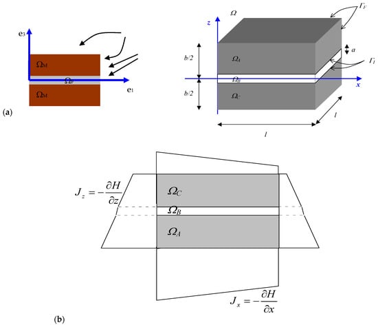
Figure 11.
(a-left): Schematic of a “unit” block Ω containing a single “fracture” ΩF sandwiched between two layers of porous matrix ΩM. (a-right): The fractured matrix block, with explicit indication of fracture aperture and matrix layers thicknesses. (b): Two-dimensional view of the piecewise linear head conditions, corresponding to piecewise constant gradient J along the boundaries (GRD’).
To upscale the flow on this geometry, we first look for a local velocity distribution
such that, on each sub-domain Ωk (k = A,B,C), except at the material interfaces , we have:
submitted to piecewise linear head boundary conditions of as follows:
Notations. All lower-case quantities are local microscale quantities. They are generally non constant in space. For instance, the hydraulic gradient j0 is imposed (subscript 0) but not necessarily constant in space (lower case j). In the present case, because j0 is piecewise constant, we use the notation j0(k), where index (k) describes the sub-domains.
The above condition is applied separately on each piece of the boundary (on each subdomain k = A,B,C). Note that the boundary conditions are chosen here such that h(x,y,z) is of the lowest possible order: 3) (space of continuous functions). The head field is not necessarily differentiable, or possibly, only differentiable along some directions. For this reason, the final upscaling result, although exact for these boundary conditions, is a “low order” equivalent conductivity tensor (from that point of view).
The next step is to implement mass flux continuity and pressure continuity along all “layer/layer” interfaces , that is , including at boundary points where interfaces meet boundaries, that is . For instance, in the case of a horizontal interface, the continuity relations are.
Notations for interfaces: designates all interfaces pertaining to sub-domain ; on the other hand, a notation such as can be used to denote the interface formed by the intersection of the two sub-domains and (see Figure 11).
After some manipulations, which are not detailed here, and expressing the piecewise constant gradient in terms of a constant reference gradient denoted , a unique set of piecewise linear head conditions (and gradients) is obtained that satisfies the continuity conditions, not only inside the domain but also on its boundary. The reader can verify this by direct insertion of the following equation:
These boundary conditions finally produce a piecewise constant velocity vector v(x), which can be controlled by controlling , and which satisfies mass balance and continuity conditions throughout the composite domain ():
Using this flow field, the upscaled conductivity for this special problem is obtained below.
In order to upscale this local flow problem, the average flux and gradient vectors are computed at block scale with one of the available methods, given the exact “local” flow field given by Equations (108) and (109). Thus, using the VAF method for the block scale flux and the VAG method for the block scale gradient, we obtain respectively (There are in fact several ways to proceed with this average. Here we consider the Volume Averaged Flux (VAF). However, in Appendix IX of Canamon [82], the approach based on Vectorial Surface Flux (VSF) is also presented (which may be useful for comparison purposes).):
Denoting ϕ the volumetric fraction of the inner “fracture” layer within the block, and (1 − ϕ) the volumetric fraction of the matrix, we obtain the block scale (VAF) flux vector as:
and inserting the block scale (VAG) gradient , we obtain a “Darcian” linear tensorial relation between the macroscopic flux and gradient vectors, as follows:
Finally, this yields the equivalent tensorial conductivity of the block in the block’s reference frame:
where the resulting principal conductivities (Kii*) can be interpreted as weighted arithmetic and harmonic means. More generally, if the 3D block is oriented at angle with respect to the reference frame, we obtain:
where: (ni, i = 1,2,3) are the components of the unit vector n normal to the layers; KA and KH are the weighted arithmetic and harmonic mean conductivities (defined above).
Specialization: Equivalent Kij for a Single Fracture Block with Impervious Matrix
Finally, it is interesting to specialize the above result to the case of a single fracture traversing an impervious block with zero matrix permeability; this is a very basic building piece of any “fracture network”. Thus, we set kM = 0, and we obtain as a result a tensorial block conductivity of the form:
where ϕ is simply the volumetric fraction of the single “fracture” within the impervious block. For a Poiseuille fracture, the conductivity in Equation (116) is the Poiseuille conductivity parallel to the fracture plane (law of cubic aperture). However, if the fracture is made up of (or filled with) a coarse isotropic porous material, then we set in Equation (116) to represent the local isotropic Darcy conductivity inside the coarse “fracture” medium.
5.2. Exact Flow Solution for Two Anisotropic Layers under Piecewise Linear Head Conditions (GRD’)
Renard ([80], Appendix B) developed a similar 3D solution under piecewise linear head conditions for a two-layer Darcian medium with fully non-diagonal permeability tensors, one in each layer. Thus, let us consider a composite medium made of two adjacent homogeneous 3D blocks, as shown in Figure 12.
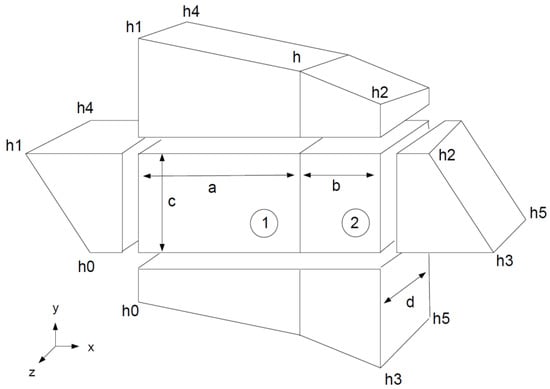
Figure 12.
Composite medium made of two rectangular cuboid blocks. Definition of the geometry and of the boundary conditions.
The two blocks have the shape of a rectangular cuboid, and they share a common face. They both have a constant hydraulic conductivity tensor and . The aim of this section is to derive an analytical expression for the equivalent conductivity tensor that represents globally the composite block under the assumptions (1) that the local conductivity tensors and are symmetrical definite positive and constant in each block and (2) that the local scale-specific discharge rates and are different but spatially constant in each block (the streamlines are straight lines in each block). Under these assumptions, the head gradients are constant (but different) within each domain, and one can derive an exact analytical solution. A gradient in three dimensions can be defined by the values of four heads at four locations. To define these gradients and the continuity of head values at the boundary between the blocks, we introduce head values at some corners of the domain (see Figure 12). The values that are not named in the figure depend uniquely on the ones that are defined, and it is therefore not needed to introduce them.
To obtain the solution, the first step consists in defining the boundary conditions, which ensures that assumption (2) is honoured. To get the most general solution under this framework, we assume in addition that none of the head gradient component is equal to zero. With the geometry and notations introduced in Figure 12, the expression for the head gradient in block 1 (left side) is:
and for the head gradient in block 2 (right side), we have:
The continuity of the heads at the boundary between the two blocks implies the equality of the components of the gradient in the y and z (2 and 3) directions for the two blocks, and therefore we observe that we have:
To identify the head value noted h in Figure 12, we write the continuity of the local scale flux normal to the interface between the two blocks. This implies that the x component of the local scale Darcy velocity in the two blocks must be equal.
In the notation , the subscript represents the th component of the velocity vector, and the superscript allows to identify the block; is the x component of the local Darcy velocity in block 2. By applying the local scale flow equation on both blocks, one obtains the equality:
from which the unknown h can be isolated. Hence:
Then, we define the equivalent conductivity as the conductivity of a homogeneous block such that
and such that the upscaled fluxes that traverse all the sides of the homogeneous medium should be identical to the ones traversing the composite heterogeneous medium. Let us first express the component of the Darcy velocity in the first direction (or rather, its opposite . It is identical in both blocks and equal to:
If we replace h by the result of our previous computation (Equation (123)), we obtain the expression
In the equivalent homogeneous medium, the same flux is expressed as
Similarly, the second component of the upscaled Darcy velocity (along the y direction) must be equal to the mean of the total flux passing through the composite block in that direction.
where represents the local scale Darcy velocity component in the second direction (the y direction) in the first block, and represents the local scale Darcy velocity component along the second direction for the second block. Replacing the local scale velocities by their expression, we obtain
A similar computation for the third component of the upscaled Darcy velocity gives:
to be compared with:
Finally, using these expressions, one can estimate all the components of the equivalent conductivity tensor as follows:
These relations generalize the classical arithmetic and harmonic mean for a layered medium. One can check that Equation (132) reduces to a diagonal tensor with the arithmetic mean in directions y and z when the cross terms of the local conductivity tensors are zero. We also note that Equation (132) reduces to the equations that were presented by Kasap and Lake [105] for an analogous tensorial problem in 2D.
6. Numerical Experiments
Among the different techniques that were presented in the previous section on criteria for the equivalent conductivity, it is not obvious to know in advance which upscaling techniques (if any) might satisfy some other criteria in addition to those directly used for defining the equivalent conductivity.
For example, when one uses the DIAG method (criterion) with linearly varying head conditions (boundary conditions), a question that can be asked is the following: “is the TDP criterion also verified?”. Similarly, what about the Net Surface Flux when defining K using the Volume Average Flux? Other important questions are whether the resulting equivalent conductivity is a true second rank tensor, whether it is symmetric, and whether it is positive-definite? (Briefly, is a “true” second rank tensor if its components are transformed according to tensorial transformation rules under a rotation of the coordinate system; is a non-symmetric tensor if ; and is positive definite if its symmetric part is positive-definite. Finally, a symmetric matrix is positive-definite if any quadratic form is strictly positive for all non-zero vectors .)
In this section, we apply the different upscaling methods on numerical examples, and we explore the properties of the methods. The cases are chosen to illustrate not only the standard situations, but also the pathological situations that can occur, and to understand them. This series of numerical experiments provides counter examples allowing to know when some criteria or properties are not systematically satisfied. (In the next Section 7, we will concentrate on analytical proofs to demonstrate the general validity of some numerical observations made in this section concerning the properties of the various versions of equivalent conductivity.)
6.1. Continuous and Composite Media in 2D
In the case of continuous and composite media, the detailed and global flow calculations, required to numerically compute the equivalent permeability tensor and to check the accuracy of the methods, were conducted either with the commercial finite element code FEFLOW (http://www.feflow.info, accessed in 18 June 2022) or with MATLAB routines developed by us for the purpose of this work. In both cases, we used standard bilinear rectangular finite elements.
6.1.1. Experimental Setup, Types of Media, and Methodology
Numerical tests have been conducted in two and three dimensions, but for illustration purposes we present only two-dimensional results. Here, we study 12 synthetic media with different spatial distributions of hydraulic conductivities. These media are represented in Figure 13.
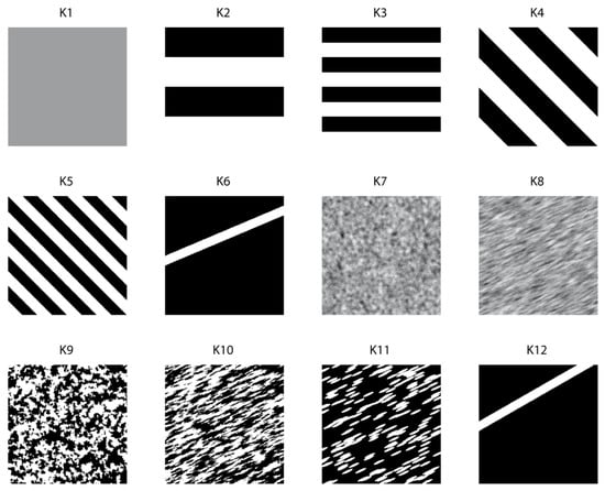
Figure 13.
The twelve two-dimensional synthetic samples of porous media proposed for analysis. The white and light grays represent high conductivity values, while the black and dark grays represent low conductivities.
The first test sample, denoted K1, is a homogeneous anisotropic medium; the local conductivity is a constant tensor represented by a matrix with non-zero of off-diagonal terms. All the other samples K2 to K12 are heterogeneous, and their local conductivity is isotropic, represented by a spatially varying scalar . However, in spite of local isotropy, some of these samples can exhibit anisotropic geometric structure due to the spatial organization of the local conductivities. Media K2 to K6 are stratified (or multilayered), with a contrast of conductivities of 100. Media K7 and K8 are multi-Gaussian random media, with a lognormal probability distribution of hydraulic conductivities, respectively, with isotropic structure (K7) and anisotropic stratified structure (K8). The random medium K8 exhibits an inclined geometrical anisotropy (or statistical anisotropy). Media K9 and K10 are, respectively, isotropic and anisotropic random binary media, having the same proportions of the two phases. (The term “phases” is understood here, for binary media, in the sense of material phases (e.g., high permeability sand for the white phase and low permeability clay for the black phase). In all cases, the porous media are considered to be water-saturated (or saturated with a single fluid phase).) Medium K11 is a random Boolean medium made up of porous matrix (black) with “anisotropic” lenticular inclusions of elliptic shape. Medium K12 is similar to K6, but here, the unique conductive stratum connects two adjacent perpendicular faces (instead of two opposite parallel faces in K6).
For all these block samples of porous media, a reference hydraulic conductivity tensor can be estimated either with an exact or an approximate analytical formula (see Table 3). In all the cases, the reference hydraulic conductivity assumes that the medium is infinite and that the flow is uniform through the medium. For the stratified media, the reference equivalent conductivity is calculated using the arithmetic and harmonic means for the directions parallel and perpendicular to the strata.
Table 3.
Reference conductivity tensors for the twelve two-dimensional synthetic media.
For the random multi-Gaussian medium and for the binary isotropic medium with identical proportions of high and low permeability cells (K7 and K9, respectively), the exact effective conductivity is the geometric mean [30].
For the multi-Gaussian and binary anisotropic media (K8 and K10, resp.), we use the geometric mean corrected by the anisotropy factors proposed by Ababou [68] and Ababou ([106], Appendix B therein):
where represents the geometric mean, the variance of the neperian logarithm of conductivity, the correlation scale in the i direction, and the arithmetic mean of the correlation scales. The same formula was also applied to the anisotropic Boolean medium K11 with elliptical inclusions. Finally, note that all media except K1 have locally isotropic conductivity ; on the other hand, several of the proposed sample media such as K8, K10, and K11 are structurally or statistically anisotropic, although their local conductivity is isotropic (scalar).
For each of these 12 samples of porous media, 8 equivalent conductivity tensors were computed numerically using the methods described in the previous section. These eight conductivity tensors correspond to four averaging methods—or interpretation methods (DIAG, NSF, VSF, and VAF)—and to two types of boundary conditions (linearly varying head and permeameter type).
To analyze the results, we use several measures. First, we define a dimensionless error norm ε by computing the Frobenius norm of the difference between the estimated equivalent conductivity tensor and the reference tensor. The Frobenius norm is also called Euclidian norm [107]. The Frobenius or Euclidian norm was chosen because it can be used to compare two tensors globally. It is close to zero when the eigenvalues and eigenvectors of the two tensors are close. It is defined as follows:
where N = 2 in 2D, or N = 3 in 3D. The Frobenius norm can also be expressed as follows in terms of the eigenvalues of , i.e., the principal conductivities (which are independent of the chosen coordinate system): . Interestingly, it can also be proved that the Frobenius norm of a symmetric definite positive tensor is the trace of the “square-root matrix” defined by . In other words, we have the identity: . The proof is obtained by expressing B in the form where is lower triangular and is diagonal, and using the principal basis where is represented by the diagonal matrix .
Secondly, we define the error ε as the Frobenius norm of the difference between the “estimated” and the “reference” equivalent conductivity, and we normalize it by the norm of the reference conductivity, namely:
Thirdly, we estimate the relative magnitude β of the anti-symmetry of the resulting equivalent tensor:
Both criteria ε and β are useful.
On the other hand, we use other comparison methods, based on the upscaled flow field (V); the estimated equivalent K tensor is used to compute again the flow field with the same boundary conditions that were used to compute the small-scale flow field (v). We also compare the total dissipated power and the fluxes obtained with the equivalent medium (equivalent conductivity K) and with the original heterogeneous medium (local conductivity k).
6.1.2. Comparisons with the Reference Permeability Tensors for 12 Porous Samples
In Figure 14, we first show for each 2D porous sample (K1, K2, …, K12) the relative difference between the reference value and the computed tensor for all the techniques that we tested.
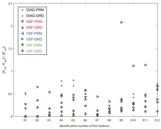
Figure 14.
Comparison between the twelve estimated (Kest) and reference (Kref) hydraulic conductivity tensors for the 2D cases; the ordinate represents the normalized Frobenius norm of their difference, and the abscissa represents the different types of media (12 porous samples labeled by their identification number).
The first striking characteristic that can be seen in this graph is that there is no obvious and systematic classification of the methods. The volume surface flux with linearly varying head (VSF-GRD) seems to provide very often a tensor far from the reference values, but at the same time it performs better than many other techniques for the first case (medium K1). Some techniques seem to be more reliable than others, but the classification is often changing depending on the type of heterogeneous medium. None of the techniques systematically provides a value equal or very close to the reference.
It is therefore important to understand more precisely what are the physical mechanisms that control those differences. Let us start with the homogeneous anisotropic case (Test case 1 denoted “K1” in Table 3).
- ▪
- For the homogeneous anisotropic medium, when applying linearly varying head boundary conditions, all the methods correctly identify the permeability tensor.
- ▪
- With permeameter (PRM) boundary conditions, only the VAF+VAG method provides the right answer (the reference flow field and the equivalent conductivity tensors are displayed in Figure 15a–c). We did not plot the DIAG method here since it is obvious that it will not properly capture the anisotropy. Since the homogeneous domain is anisotropic, the flow lines are not perpendicular to the head isovalues. The geometry of the flow is distorted in such a way that it minimizes the total dissipated power within the media accounting both for the boundary conditions and the anisotropy imposed by the conductivity tensor. As a consequence, there is a difference between the mean head computed on the two no-flow boundary conditions, and there is a deviated component of the mean Darcy velocities within the domain.
- ▪
- When we compute the net surface flux (NSF), these inclined components cannot be identified since the two faces in the direction perpendicular to the vertical component are forced to be impervious. The head gradient in the domain is still correctly estimated, using the volume average gradient (VAG), and allows identifying an off-diagonal term in the equivalent conductivity tensor. As a result, KNSF correctly captures the direction of anisotropy (see Figure 15c), but the magnitude of the maximum principal value is underestimated and the perpendicular component is overestimated (the ellipsoid is closer to a circle than the reference).
- ▪
- In contrast, the vectorial surface flux (VSF) averages directly the specific discharge vectors “v” on the faces of the sample and overestimates the vertical component because “v” tends to be very inclined along the boundary. Indeed, the “v” vector inside the domain (near no flow boundaries) is much less inclined but not sampled by the VSF. We observe that the VSF technique properly identifies the main directions of anisotropy, but in this case, it overestimates the maximum principal component and underestimate the smallest component (the ellipsoid is flattened as compared to the reference one).
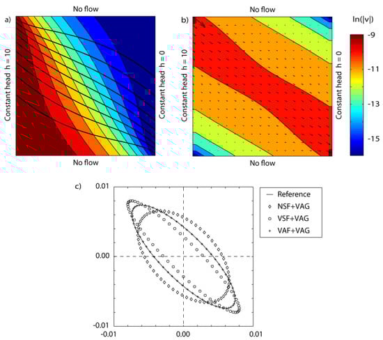
Figure 15.
Illustration of the head field (a) and velocity field (b) in a homogeneous anisotropic medium (sample K1) computed with permeameter type boundary conditions (PRM). The medium is homogeneous, as K1, but it has been chosen here with a different orientation to better illustrate the distortion of the flow field. Its main axis of anisotropy in this figure is inclined at –45 degrees, , . Anisotropy ellipses are shown below in plot (c). These ellipses represent the square root of flux directional permeability [77] obtained here with the NSF, VSF, and VAF criteria. The ellipses axes are aligned with the principal directions of anisotropy, and their principal radii are the square roots of the principal values of conductivity.
A brief conclusion from this first experiment (K1: homogenous anisotropic medium) is the following: linearly varying head boundary conditions (GRD) and volume average flux (VAF) are best. However, this is not always true, depending on the type of medium, as will be seen in the next example.
We now examine the stratified or layered medium K2 displayed earlier in Figure 13 The results are shown in Figure 16. One can observe a behavior that is opposite to the one described in the previous paragraph. For test K2, all the techniques based on PRM boundary conditions are converging toward the reference value, whereas the techniques using GRD boundary conditions leads to a significant error. More precisely, for sample K2:
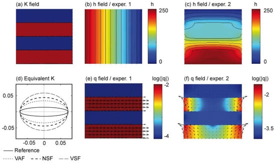
Figure 16.
Medium K2 with linearly varying head boundary conditions (GRD): (a) K field, the red layers are the high permeability layers. (b,c) Head distribution in the domain for the two flow experiments. (d) Ellipsoids of the square root of flux directional permeability obtained with the VAF, NSF, and VSF criteria. (e,f) Darcy velocity fields for the two flow experiments; the background color represents the norm of the Darcy velocity.
- all the techniques identify properly the principal directions of anisotropy;
- all the techniques also estimate correctly the largest principal component K// parallel to strata (arithmetic mean of local permeabilities);
- in the perpendicular direction, we expect to obtain for K⊥ the harmonic mean permeability; however, all the methods using GRD boundary conditions overestimate K⊥ significantly (Figure 14); the overestimation is maximum for VSF, minimum for VAF, and NSF lies in between.
The reason for this overestimation of K⊥ is the presence of flow cells on the sides of the most permeable layers in the K2 sample (see Figure 16e,f). Water is entering the high permeability layers at their base and leaving them laterally because of the prescribed head gradient along the boundary. The same behavior would occur if the block would be immersed in a medium with intermediate conductivity: the flow would converge toward the high conductivity layer and diverge around the low conductivity zones. The consequence is that the total flux perpendicular to layers is much higher than it would be if the layers were infinite, and therefore we obtain a systematic overestimation of the equivalent conductivity K⊥ perpendicular to layers.
Note: the opposite situation arises when forcing the flow through flux conditions instead of head conditions; this is discussed in Section 6.1.5 comparing flux immersion vs. head immersion conditions.
Is this apparent overestimation of the orthogonal K⊥ really a problem? In fact, one could argue that it is not the block permeability K⊥ that is overestimated, but rather that the reference used for comparison underestimates the true perpendicular block conductivity. Indeed, the reference used here assumes an infinite extension of layers, and/or a set of infinitely thin layers. In fact, the K2 test contains just a few thick layers of finite extension, and the local 2D configuration of the flow near the boundaries suggests that indeed, the equivalent perpendicular K⊥ is truly larger than the harmonic mean in this particular case (Figure 16f). Overall, this discussion brings about the need for using skin immersion (or border regions) when computing the equivalent conductivity [55], e.g., in the case of thick layers with respect to block size. The magnitude of these differences will probably decrease when the number of layers increases (compare samples K2 and K3 displayed earlier in Figure 13); this will be due to a decrease in the size of the rotational flow cells, such as those observable at the intersection of domain boundary and layer interfaces in Figure 16f.
Continuing with the comparison of the computed permeability tensors versus reference conductivities, we now consider media K3 and K4 (which have inclined layers). We find as expected that the errors are maximal with the DIAG method compared with all other methods.
For the random multi-Gaussian fields (concerning the spatially correlated MultiGaussian random fields K7 and K8, the notions of local vs. structural or statistical anisotropy should be distinguished. Both K7 and K8 represent spatial distributions of locally isotropic conductivity . However, the first one (K7) is also isotropic structurally (statistically), while the second one (K8) is anisotropic structurally (statistically).), the isotropic field (K7), and the anisotropic field (K8), which have fairly small spatial correlation lengths with respect to block size, all the techniques are reasonably good except the VSF+GRD method (i.e., Vectorial Surface Flux “VSF” combined with linearly varying head or fixed gradient condition “GRD”).
Finally, the highest differences between the computed equivalent conductivity and the reference values are observed for binary random media (K9, K10, K11) when using the VSF+GRD method (vectorial surface flux with linearly varying head conditions).
6.1.3. Analysis of the Degree of Anti-Symmetry of the Computed Tensors
Figure 17 shows for each numerical experiment (test media K1, …, K12) the relative magnitude of the anti-symmetric component of the resulting permeability tensors, normalized by the Frobenius norm of the full tensor (Equation (134)). It can be seen that anti-symmetry arises with some of the methods (not all), and only for some types of heterogeneity (not all).
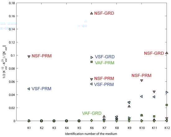
Figure 17.
Magnitude of the antisymmetric component of the equivalent permeability tensors, relative to the Frobenius norm of the full permeability tensor.
We observe that anti-symmetry arises in the simplest test case (K1: homogeneous anisotropic medium) when applying the NSF method with permeameter (PRM) boundary conditions. This is not surprising, since the NSF method cannot deliver in a single experiment the two components of the average Darcy velocity when permeameter (PRM) boundary conditions are used.
For all the stratified media, horizontal or inclined (K2 to K5), all the methods gave symmetrical tensors. Those results are related to the geometric symmetry of the media themselves, with respect to heterogeneous structure as well as domain shape.
Indeed, non-symmetry arises for medium K6 containing a single inclined stratum that is not well centered into the block. In that situation, the only method that provides a symmetric tensor is the volume average flux VAF method with linearly varying head conditions, but all other methods yield a non-symmetric tensor.
Similarly, for the multi-Gaussian and binary media (K7, K8, K9, K10, K11), all the techniques except VAF produce non-symmetric permeability tensors.
To provide a synthesis of all the previous results obtained for various 2D media, we plot in Figure 18 the different upscaling techniques on a map in terms of the degree of non-symmetry. Each technique is represented by a point whose coordinates are as follows: the x-axis represents the average normalized error over all numerical experiments (twelve different media), and the y-axis represents the average of the normalized anti-symmetric component of the computed tensors. We see clearly in Figure 18 that the Volume Average Flux technique with the Linearly Varying head is the technique that always provides a symmetric tensor and that it also has the lowest error with respect to the reference value on average over all test cases (over the limited sample of 12 blocks of porous media investigated here).
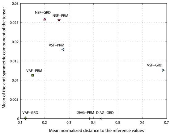
Figure 18.
Synthetic representation of the comparison between the reference and the numerically estimated equivalent conductivity tensors, in terms of the degree of anti-symmetry. The abscissa of a point in this figure represents the average of the norm over the twelve 2D blocks of porous media defined in the text. The ordinate represents the mean degree of anti-symmetry, averaged over the twelve 2D media.
6.1.4. Net Surface Flux and Total Dissipated Power Criteria (Verification)
In this section, we check numerically whether the Net Surface Flux and the Total Dissipated Power criteria are verified a posteriori. For that purpose, we solve the flow problem numerically on the upscaled media. Since some approximations had to be made in order to define the equivalent K with some techniques (NSF for example), it is not obvious that the criteria are verified a posteriori.
In Figure 19, we compare the net surface flux in the x1 direction computed on the detailed heterogeneous media versus the corresponding equivalent homogeneous media with the PRM and GRD boundary conditions, and this was performed for all the media (the 12 porous block samples). The following results emerge from these graphical comparisons:
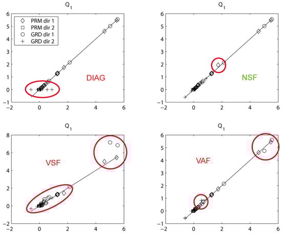
Figure 19.
Comparison between the values of the microscopic total flux Q1 calculated on the heterogeneous media (abscissa) with the total macroscopic flux computed with the same boundary conditions on the upscaled homogeneous medium (ordinate). Each graph represents all the numerical results for a given upscaling method (DIAG, NSF, VSF, VAF).
- The DIAG technique reproduces very well the Net Surface Flux in the direction of flow imposed by the boundary condition. Note, in the direction perpendicular to the main gradient (GRD case), the fluxes are necessarily zero because the DIAG method neglects the off-diagonal term of the conductivity tensor.
- The NSF method is almost perfect, but still one can see that with PRM boundary conditions there is a slight discrepancy due to the approximation discussed earlier.
- The VSF method shows the highest dispersion and seems to be the least accurate.
- The VAF method seems good overall but shows some slight difference between the fluxes in the case of the GRD boundary conditions. Surprisingly, it seems that the VAF perfectly reproduces the fluxes in the case of PRM conditions.
Similar comparisons are also shown in terms of Total Dissipated Power (TDP) in Figure 20. It can be seen that, among all the techniques that we tested, only the VAF method accurately reproduces the TDP criterion. Among the other techniques, the DIAG and NSF methods perform rather well overall, while the VSF method is less accurate.
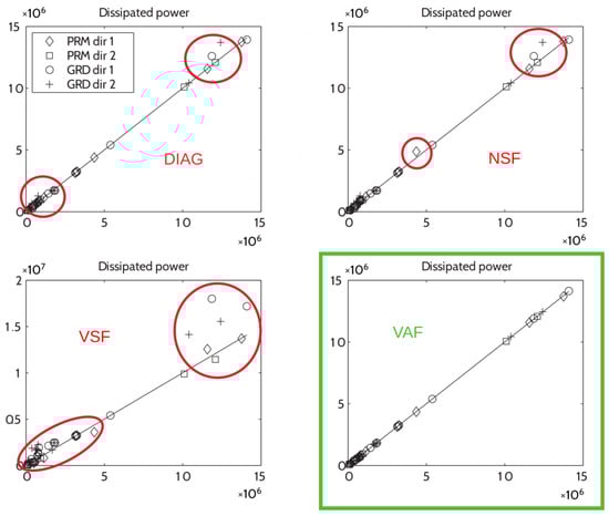
Figure 20.
Comparison between the total microscopic dissipated power (P) computed on the heterogeneous media (abscissa) with the total macroscopic power calculated with same boundary conditions on the homogeneous media (ordinate). Only the VAF method with PRM and GRD boundary conditions ensures the equality of the dissipated powers.
All these numerical/graphical results are also summarized in Table 4.
Table 4.
Main properties of the upscaling techniques discussed in this paper.
6.1.5. Flux Immersion Conditions: Comparisons with Linear Head Immersion
This section discusses prescribed “flux immersion” boundary conditions versus the prescribed head conditions. More precisely, “flux immersion” conditions correspond to the case where the flow is forced by immersion of the porous block in a flux vector field (using the normal fluxes as BC’s)—to be compared to hydraulic gradient immersion (where linearly varying heads are imposed on the boundary).
We use a horizontally layered block K2bis as a prototype case for this discussion. This block is similar to a thickly fractured block comprising three layers (M; F; M), with the “Fracture” layer sandwiched between the “Matrix” layers as illustrated earlier in Figure 11. The relative permeabilities and thicknesses of the three layers are (kM; kF; kM) = (1; 1000; 1) and (eM; eF; eM) = (9; 2; 9). The averaging method used to interpret the flux immersion experiment is VAF for the flux and VAG for the gradient. The results obtained with flux immersion , compared to linear head or “gradient immersion” , are the following:
These results can be interpreted by comparing them with the reference tensor:
Note that the equivalent block permeability is expressed in the reference frame aligned with the layers, with KA and KH denoting the weighted arithmetic and harmonic means of the permeabilities of the three layers (The arithmetic mean “KA” should not be confused with the anti-symmetric part also denoted “KA” in other sections.). This reference tensor was shown in Section 5.1 to be the exact equivalent permeability of the block under piecewise linear head conditions, or equivalently, under piecewise constant gradient conditions (and therefore also under piecewise constant flux conditions as well). Comparisons with the GRD and FLX numerical experiments show that:
- ▪
- gradient immersion (GRD) significantly overestimates the permeability orthogonal to layers (K⊥ ≈ 10.8 >> 1.11);
- ▪
- flux immersion (FLX) drastically underestimates the permeability parallel to layers (K// ≈ 2.3 << 100.9).
These results are illustrated in Figure 21 and they confirm experimentally that the two tensors are ordered by the relation in the following sense: matrix if matrix (B-A is semi-definite positive). Pouya et al. [43,51,85] proved analytically in the continuous case the same inequality .
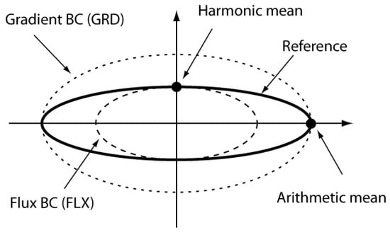
Figure 21.
Schematic representation of the 3 permeability tensors ellipsoids for a finite 3 horizontal layers block (matrix/fracture block).
Furthermore, the tensors KGRD (obtained under gradient immersion conditions, “conductive upscaling”) and KFLX (obtained under flux immersion conditions, “resistive” upscaling) are bounding the reference tensor .
From a theoretical point of view, the flux immersion and hydraulic gradient immersion experiments can be analyzed in the light of other theoretical approaches, the first one (A) dealing directly with a flux governing equation to analyze local flow, and the second one (B) considering together the conductivity upscaling problem (under gradient conditions) and the “dual” resistivity upscaling problem under flux conditions [75]. These approaches were outlined earlier in Section 2.2.2 and Section 4.3 and are also described in detail in Appendix A.2.
However, in the light of the resistivity approach from Fadili and Ababou [75], the result can be re-interpreted as [Rij]−1 ≤ [Kij] if we choose to denote [Rij]−1 the upscaled resistivity (under prescribed velocity) and Kij the upscaled conductivity (under prescribed gradient, or linearly varying head). Thus, if we admit that the equivalent [Rij] 1 and Kij tensors correspond to two distinct flow experiments with boundary conditions FLX and GRD (respectively), then, the two tensors do not necessarily match, and they are always ordered as indicated above.
6.2. Simple 2D Fracture Networks
In this section, we use simple 2D fracture networks (Figure 22 and Figure 23) to illustrate further the properties of the different techniques. Only linearly varying head boundary conditions are used in this section.
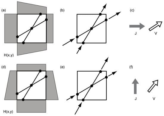
Figure 22.
Schematic of a fracture network and the Darcy velocities corresponding to a flow experiment with a prescribed horizontal gradient (a–c) or a prescribed vertical gradient (d–f). Figures (a,d) represent the network and the two sets of boundary conditions. Figures (b,e) represent the velocity vectors in the individual fractures. Figures (e,f) represent the prescribed mean gradient and the resulting mean velocity. In both cases, the Darcy velocity is deviated toward the principal direction of anisotropy, which is oriented at 45 degrees.
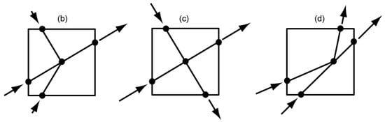
Figure 23.
Schematic of three simple fracture networks (b–d), with the Darcy velocities corresponding to a flow experiment with a constant horizontal gradient. All the fractures have the same aperture. The lengths of the 4 fractures are identical in cases b and c, and the local conductivities are also identical. The letters (b–d) above the graphs correspond to the cases discussed in the text and to the results reported in Table 5.
First, we want to illustrate when non symmetry occurs. For that purpose, we start with a simple medium (Figure 22) such that all the techniques deliver a symmetric tensor with a strong off-diagonal component (Table 5, case a). After having described this medium and the corresponding results, we will modify it to show when the non-symmetry occurs.
The initial medium contains two fractures (Figure 22) intersecting exactly in the center of the domain. The medium is symmetric around a line going through the center of the domain and inclined at 45 degrees. On Figure 22a, we see the Darcy velocities computed for a linear gradient oriented along the x1 direction. J is horizontal; the average velocity cannot be in the same direction due to the anisotropy and is deviated toward the principal direction of anisotropy at 45 degrees (Figure 22b). When the prescribed gradient is rotated by 90 degrees (Figure 22c), the velocity is again deviated toward the principal direction of anisotropy at 45 degrees (Figure 22d). Due to the geometrical symmetry of the fracture system, the flux is identical to , and this directly ensures the symmetry of KNSF (see Table 5, case a). Still because of the geometrical symmetry, the vectorial surface fluxes and are identical; KVSF is symmetric too as well as KVAF (Table 5, case a).
We now consider the fracture network (b) on Figure 23. Compared to the previous figure (Figure 22), here one boundary point of the upper left fracture has been moved toward the left. This has been done to ensure that the total flux in the vertical direction becomes zero during the experiment with a horizontal gradient, while keeping a value different from zero in the perpendicular experiment. As expected, the result is that KNSF is asymmetric (Table 5, case b). The other averaging techniques still provide a symmetric tensor as shown in Table 5.
If we continue to perturb the initial setup and move now the lower right fracture in order to obtain a perfect cross with perpendicular fractures but not aligned with the coordinates’ axis (Figure 23c), the asymmetry becomes even stronger for KNSF with opposite off diagonal terms 0.84 and −0.84 (Table 5, case c). These results are obtained because when the gradient is prescribed in the horizontal direction, the fractures are oriented at an angle close to 40 degrees upward but the net fluxes on the faces are such that the estimated mean velocity with the NSF method is oriented downward. When the gradient is rotated by 90 degrees, again the mean velocity estimated with the NSF criteria is inclined toward the right. In both conditions, the velocity field always rotates with respect to the prescribed gradient, and the only way to describe that behavior is to use an anti-symmetric tensor. We also note that in this example, the symmetric part of KNSF is perfectly diagonal. This is in close agreement with the other averaging techniques which deliver a diagonal tensor (Table 5) and therefore consider the medium as isotropic.
With the previous examples, KVSF and KVAF was always symmetric. However, in some situations, it happens that the tensor becomes asymmetric but with a moderate anti-symmetric component. To illustrate that behavior, we show an example in Figure 23 and Table 5 case (d); it is based on the initial case (a) displayed in Figure 22, except that the central node was moved in order to break the symmetry of the fracture network. In this new situation (Figure 23 and Table 5 case (d)), both the NSF and VSF criteria give a non-symmetric K tensor. Only KVAF is symmetric.
The next example (Figure 24a) illustrates when a negative principal value can occur with the VSF method. The fractured sample is symmetric around a horizontal line splitting the domain in two equal halves. In each half domain, a two-part fracture enters the domain from the left and leaves it from the side. When prescribing GRD boundary conditions, we impose a constant head difference between the entry and outlet of the fracture. The flux through the fracture is constant, but the orientations of the inflowing and outflowing vectors are different and even almost opposite. More precisely, the orientation of the flux entering the block from the left is more inclined than the orientation of the outflowing edge (Figure 24a). As a consequence, the sum of the two vectors gives a backward horizontal component (Figure 24b). Due to the symmetry, the sum of those vectors for the two fractures gives a zero vertical component. Overall, while the prescribed gradient should force a forward flux, the VSF method computes a mean flux that is oriented backward and therefore leads to a negative value of K11 (Table 6).
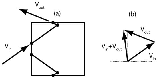
Figure 24.
Schematic of a fracture network leading to a negative diagonal component for VSF. (a) Geometry of the network and Darcy velocities for the two upper edges of the network when a horizontal gradient is prescribed. (b) Geometrical representation of the sum of the two vectors represented in subplot (a).
Table 6.
Hydraulic conductivity tensors computed on the networks displayed in Figure 24.
On the other hand, in the same situation the forward flux is estimated properly by the Net Surface Flux and the Volume Average Flux methods, and both methods yield a positive definite K, with more or less similar positive values for K11 (Table 6).
To conclude, this example shows that the VSF method does not necessarily provide a positive-definite tensor.
In the last example (Figure 25), we consider two set of fractures having a fixed spacing and fixed orientations.
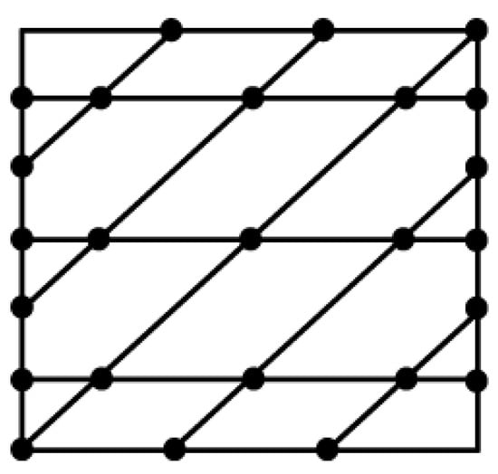
Figure 25.
Schematic of a fracture network made of two sets of equally spaced and parallel fractures.
Based on this geometry, we analytically compute the reference equivalent permeability tensor for an infinite medium [59,60]. Briefly, this reference permeability is obtained by a superposition of fluxes (Q in m2/s). In 2D, the direct superposition of fluxes projected on the fracture segments yields, for each fracture f:
Summing over all fractures (f = 1, …, N) and using indicial notation, this yields:
The equivalent tensorial transmissivity (m2/s) emerges). Finally, dividing by domain cross-sectional area (or domain length in the 2D case), e.g., for the case of a single set of parallel fractures, there emerges a mean fracture spacing , and one finally obtains (for the single set of parallel fractures):
where Kij is the equivalent hydraulic conductivity, obtained here explicitly. For a set of two parallel families of fractures, these formulas specialize as follows:
where N is the number of families of fractures, I is the identity matrix, for each family of fracture, is the unit vector normal to the fractures (they are all parallel), its transpose, is the spacing between two fractures, and the aperture.
By comparing the analytical results with the numerical ones (Table 7), we find that all the components of the tensor are correctly estimated only if we use the VAF method. The NSF method tends to underestimate the off-diagonal terms and the smallest principal value. The VSF method overestimates all the components of the tensor.
Table 7.
Hydraulic conductivity tensors computed on the networks displayed in Figure 25.
7. Analytical and Algebraic Proofs of the Properties of Equivalent K
In the previous section, we have seen some systematic patterns in our numerical results. While some techniques were shown that do not provide symmetrical tensors or do not satisfy the criterion of total dissipation of energy, others were always satisfying those criteria. These results are summarized in Table 5. In this section, we provide some analytical studies and proofs of the properties of the equivalent permeability tensors defined previously. The results of this work are also listed in Table 4 to confirm, when possible, the numerical observations.
7.1. DIAG + PRM ensures NSF and TDP
In the case of permeameter type boundary conditions, the Total Dissipated Power (TDP) criterion can be expressed very simply as follows (P is the dissipated power):
This relation is derived in detail in the Appendix A.7.4 by replacing the volume integral in the definition of the TDP by a surface integral. All the terms on the no-flow boundaries vanish and only the terms on the boundaries with a prescribed head remain. Since the head is constant on those boundaries, it can be taken out of the integral and the whole equation simplifies to Equation (144) both for the heterogeneous and homogeneous media. The DIAG method ensures that the total flux in the direction of the imposed gradient is identical in the homogeneous and heterogeneous media , and the prescribed head difference between inlet and outlet is also identical on both media . Therefore, the total dissipated power criterion is always verified when we compute the equivalent conductivity using the DIAG + PRM method.
Of course, this technique does not allow computing the off-diagonal components of the tensor and therefore the result may be highly inaccurate if the principal direction of anisotropy of the heterogeneous medium are not aligned with the faces of the block. In the laboratory, the presence of anisotropy can be tested by measuring the heads on the sides of the block and computing the head gradient in the direction perpendicular to the main flow. If this gradient is not equal to zero, then it is a clear indication that the sample has not been well oriented and that the resulting diagonal tensor will be inaccurate (Renard et al., 2001).
7.2. VAF + GRD Implies TDP
In the case of Linearly Varying Head boundary conditions, the total dissipated power can be expressed for any geometry as follows (see Table 2 and Appendix A.7.2):
As described in Renard [80] or Pouya and Fouche [43], the same formula can be applied both for the microscale and the homogenized macroscale problems; also, because the volume average flux criterion with linearly varying head enforces , a similar equality holds for the dissipated power as a direct consequence of the VAF criterion:
This last relation states the equality of the volume averaged dissipated power of (i) the microscale medium and (ii) the homogenized macroscale medium.
7.3. Symmetry of K for VAF + GRD
Using VAF for averages (Volume Averaged Flux) and GRD for boundary conditions (gradient, i.e., linearly varying head condition), together, ensures the symmetry of the equivalent conductivity tensor .
This was shown by several authors including Pouya and Fouche [43] for fractured media. We briefly present the proof in a slightly different form, with a tensorial local conductivity k(x). The proof is based on the principle that a tensor is symmetric if for any pair of vectors J and J’, the scalar products and are equal. (Note that J’ is just another vector, it is not the transpose of J. In this text, the notation for the transpose a vector is not J’.)
To obtain the result, we consider two flow experiments in which and are the prescribed boundary conditions, h and h’ are the head solutions of the flow problems for those two boundary conditions, and v and v’ are the corresponding Darcy velocities. The local hydraulic conductivity k is assumed to be a symmetric tensor, and therefore we can write the following equality:
By Darcy’s law, the left term of the previous equation can be written as the divergence of the product hv’:
Now, since we are looking at the VAF method, we integrate the above equation over the domain of interest:
Additionally, since we are using the GRD type of boundary condition , we can insert it as follows (recall that the global hydraulic gradient is defined as ):
The first integral vanishes because , and the second integral can be identified as the volume average flux (see Table 2). Therefore, the volume average of equation (Equation (99)) is equal to
The previous result is obtained using the definition of KVAF, and the fact the volume average gradient of h’ is equal to −J’, in addition to Darcy’s law.
Finally, exactly the same averaging and derivation can be made on the right-hand side of Equation (147), and therefore we obtain the following identity, implying that KVAF is symmetric.
7.4. VAF + GRD Is Positive Definite
KVAF is symmetric when it is computed with GRD, but it is also positive and definite. This is a direct consequence of the fact that under the GRD boundary conditions, the VAF criteria ensures that the Total Dissipated Power is identical in the upscaled medium and in the heterogeneous medium. Indeed, one can show that KVAF is positive and definite if for any vector J different from 0 the following quadratic form is always positive:
This is always true because for whatever J, the expression above is proportional to the Total Dissipated Power in the medium if we apply linearly varying head boundary conditions (GRD conditions). Since the small-scale hydraulic conductivity tensor k is assumed positive definite, the total dissipated power on the heterogeneous medium (left hand side of equation below) is strictly positive when the gradient imposed to the block is different from zero.
The right-hand side of the above equation is the Total Dissipated Power on the upscaled medium, which is equal to the TDP on the homogeneous medium. The fluid density and the acceleration of gravity are strictly positive; the right-hand side of the previous equation is then strictly positive, and KVAF is positive definite.
7.5. Symmetry of VAF / TDP & PRD
Concerning the symmetry property of the equivalent conductivity under VAF averaging for the TDP criterion and the permeametric PRD criterion, Boe [96] and Farmer [35] used Equation (72) to define the equivalent conductivity tensor and prove that the resulting tensor is symmetric. The result is in agreement with the numerical experiments of Durlofsky [37].
8. Discussion and Conclusions
It was seen in the preceding review and analyses that several other works in the literature have compared upscaling techniques. For instance, a large comparison exercise of upscaling techniques has been made by the Society of Petroleum Engineers. The problem included the simulation of multiphase flow in a large heterogeneous oil reservoir after applying various upscaling techniques. The results were reported by Christie and Blunt [108]. One of the findings of this exercise was that the equivalent conductivity obtained with no flow boundary conditions were providing “better” upscaled solutions than the results obtained with linearly varying heads (or gradient conditions) for their specific case study.
Here in this paper, we take a different perspective by conducting a more theoretical analysis of various approaches that have been used in the past to define the equivalent permeability tensor. We started by setting the problem in a very open manner and trying to review a broad range of definitions and practical ways to compute the equivalent permeability on finite domains or “blocks”. We then analyzed and illustrated the various methods with simple numerical experiments and with analytical proofs concerning their properties.
More precisely, the definitions of the equivalent conductivity that we considered involved different boundary conditions such as permeametric conditions, linear head conditions (or fixed gradient condition), and different equivalence criteria such as Volume Average Flux, Net Surface Flux, Vectorial Surface Flux, and Total Dissipated Power). We show that not only does the value of the computed equivalent permeability depends on the type of averaging technique and boundary conditions, but also the properties of the resulting equivalent conductivity can be different. These results were summarized in Table 4.
For a medium stratified along the axes of a rectangular block, permeameter type boundary conditions (PRM) allow to obtain the theoretical equivalent conductivity (which coincides in that case with the theoretical infinite domain “effective” conductivity). In contrast, for the same case of stratification parallel to the block’s axes, linearly varying head conditions (gradient conditions “GRD”) overestimate the smallest component of the equivalent conductivity tensor. Indeed, the permeameter imposes confining conditions that imply a no flow boundary perpendicularly to the strata, whereas linear head conditions generate small scale lateral circulation cells within the high conductivity strata, which increase flux perpendicular to strata (see Figure 16) leading to an overestimation of total flux. On the other hand, when the strata are inclined with respect to the block’s axes, linearly varying head conditions provide a better estimate, closer to the expected result than with permeameter type conditions.
Among the various criteria that can be used, the Volume Average Flux (VAF) criterion is particularly interesting because of the properties of the resulting equivalent permeability tensor:
- is always a symmetric tensor when combined with GRD (prescribed gradient), FLX (prescribed flux), or PRD (periodic) boundary conditions;
- The VAF method using GRD, FLX, or PRD boundary conditions, ensures that the Total Dissipated Power (TDP) is identical in the heterogeneous medium and in the equivalent homogeneous medium.
The numerical experiments show that non-symmetry of the equivalent tensor occurs more frequently with other equivalence criteria (NSF & VSF).
Negative values of some of the principal permeability values Kii* of the Kij tensor can occur with the VSF equivalence criterion. Recall that the principal values Kii* are the eigenvalues of Kij, and these are independent of the chosen coordinate system. With the VSF criterion, it is found that the resulting equivalent Kij tensor can be indefinite (e.g., with one negative principal value and the others positive), although it cannot be negative-definite (which is a physically sound result).
In addition to continuous and composite porous media, we have also presented partial results on equivalent permeability for some simple 2D fracture networks (Section 5.1 and Section 6.2). The algebraic properties of equivalent permeability of irregular fracture networks, represented as networks of links in 2D space, have also been analyzed by Renard and Ababou [62], Ababou and Renard [61], providing partial results for at least some of the criteria and conditions reviewed in the present paper. A more complete analysis is under way [97]. The case of networks of planar fractures in 3D space is another matter, which involves a richer class of “links” and “intersections” compared to 2D networks. We refer the reader to Noetinger and Jarrige [109] for semi-analytical/numerical approaches to 3D fracture network flow, to Rajeh et al. [64] for a semi-empirical approach to the equivalent permeability tensor of 3D fractured porous media with permeable porous matrix, and to Cañamón et al. [63], and references therein, for a generalized graph-based approach to percolation phenomena in 3D networks of planar fractures.
Recalling the possibility of using flux-based or velocity-based flow equations (Section 2.2.2 and Section 3.1, Appendix A.2), we show that the averaged version of this flow equation may not yield the same equivalent permeability than the head-based flow equations. For instance, the velocity version of Darcy’s law, Equation (7), may lead, upon averaging, more naturally, to an equivalent resistivity rather than an equivalent permeability. The challenge may then be to match, or at least to compare, the equivalent permeability from head-based equations to equivalent resistivity from velocity-based equations. A “dual” permeability-resistivity matching procedure (summarized in Section 4.3) was presented by Fadili and Ababou [75] for upscaling in the context of randomly heterogeneous media (effective properties in an infinite domain). A more general matching procedure, which we leave for future work, could be attempted for arbitrarily heterogeneous porous and/or fractured finite blocks, in combination with the various averaging operations and boundary conditions that were tested in the present work.
In closing, to sum up, we have presented in this paper a comprehensive review as well as theoretical and numerical analyses on upscaling methods and criteria, aimed at calculating equivalent block permeability tensors of heterogeneous media, and also, at evaluating the properties of the proposed upscaling criteria.
Author Contributions
Writing—original draft preparation, P.R., R.A.; writing—review and editing, P.R., R.A. Both authors contributed equally to the article and agreed to its publication. All authors have read and agreed to the published version of the manuscript.
Funding
This research received no external funding.
Data Availability Statement
Not applicable.
Conflicts of Interest
The authors declare no conflict of interest.
Appendix A
Appendix A.1. Tensorial Kij, Directional K, and Anisotropic Kij Ellipse
This Appendix presents a more detailed algebraic complement to Section 2.4 in the text, concerning second rank tensors such as the conductivity tensor , and several related concepts, including: principal axes, principal values, directional “flux” and “gradient” conductivities, anisotropic conductivity ellipses.
Appendix A.1.1. Vectors, Second Rank Tensors, and Tensorial Conductivity
Vectors, Tensors, and Transformation Rules
A vector is a first rank tensor. A second rank tensor or can be represented by a matrix, and it can be defined as follows, by considering that the tensor is a linear application from to :
or: (with implicit summation on repeated indices)
In 2D, with N = 2, the application T is also represented by a square 2 × 2 matrix:
The coefficients depend on the system of coordinates , and the change if the system is changed by a rotation . Conversely, its transpose transforms the new system into the initial system, and is called the passage matrix . In 2D, we have:
The rotation matrix and the passage matrix are orthogonal: (identity matrix).
In 3D, the passage matrix P becomes:
The transformation rule for a vector under a change of coordinate system, that is, under a rotation of the basis vectors , is as follows, in terms of the passage matrix :
Note: vectors and can represent the position vectors ( and ) in the old and new system, respectively.
The quantity is a “true” vector only if it is transformed as shown above under a rotation of the coordinate system. Otherwise, it is not a true vector. Example: if we have in the reference system and in the new system rotated by angle , then is not a true vector because it does not obey the transformation rule (it is, rather, a pseudo-vector).
Finally, the transformation rule for a 2nd rank tensor under a rotation of the basis vectors is as follows, in terms of the passage matrix :
Application to Darcy’s Law with Anisotropic Tensor
Darcy’s law is , where the Darcy velocity vector , the head gradient vector , and the conductivity tensor , are all expressed in the reference system . The notation is also used to designate the hydraulic gradient and will be used elsewhere.
We now derive the expression of Darcy’s law in a new transformed system as follows. We start with Darcy’s law in the reference system and we insert the vector transformation rules and , and then we also insert the tensor transformation rule for the conductivity. This yields:
which is just Darcy’s law in the new system , with the transformed conductivity as expected. This confirms, or proves, that the permeability tensor is indeed transformed by the rule . We also have conversely , using the fact that .
Principal System, Diagonalization
These transformation rules can be used in particular for finding the principal vectors and the principal permeability values ( without summation). In the new principal system , the conductivity tensor is expressed by a diagonal matrix with real non-negative values. Briefly, the principal vectors (eigenvectors) and the principal values (eigenvalues) of the conductivity tensor are obtained by solving the equations:
The first equation has three positive real roots () if is symmetric positive definite; the second equation consists in solving for the three principal vectors once the eigenvalues () are known. The principal basis vectors , or eigenvectors, are the column vectors of the passage matrix that takes the new principal basis into the initial basis (such that ). In the new principal basis, the conductivity tensor is represented by the diagonal matrix:
The conductivity matrix in a given coordinate system can therefore always be expressed in terms of the diagonalized matrix using the following relation, where the ’s are column vectors:
It is advisable to sort the eigenvalues (principal conductivities) in decreasing order, i.e., .
Thus, in 2D, let designate the angle between the first principal axis (associated with the first and largest principal conductivity ), and the first axis of the reference system. This angle can be determined to within an additive constant from the relation . If the eigenvalues are not ordered, here is another relation that determines independently of the ordering of principal values, but only within an additive constant : . The 2D principal conductivity values are given by:
In particular, we retrieve the identity , as it should, since the trace of a tensor is invariant under a change of the coordinate system.
Note: the above description concerns the diagonalization of a symmetric positive definite tensor (For a non-symmetric tensor, there are two distinct principal bases and two distinct sets of principal values.).
Appendix A.1.2. Directional Conductivity, and Conductivity Ellipse
If is a second rank tensor, symmetric and positive definite (or, more generally, this applies also to non-symmetric if its symmetric part is definite positive), then it can also be described equivalently in the form of a directional conductivity parallel to flux , or parallel to hydraulic gradient . They are functions of the direction vector of Darcy velocity or of the gradient , respectively. The direction angles can be used to indicate the direction: polar angle θ in 2D; spherical angles (θ, ϕ) in 3D. It can then be shown that the polar plots of these directional conductivities (or their square roots) describe an ellipse in 2D, or an ellipsoid in 3D. The conductivity ellipse contains all the information about the tensor: the principal radii are related to the principal values of , and the principal axes of the ellipse coïncide with the principal vectors of .
Directional Conductivity
Let us start again with the tensorial form of Darcy’s law, using the notation :
Let be the unit “flux” vector (aligned with Darcy velocity); then, by definition: . Similarly, let be the unit “gradient” vector (aligned with ); then by definition: . The directional “flux” conductivity () is a scalar quantity obtained by “projecting” Darcy’s law on the direction of the “flux”, as follows:
Similarly, the directional “gradient” conductivity () is a scalar quantity obtained by “projecting” Darcy’s law on the direction of the “gradient”, as follows:
Anisotropic Conductivity Ellipse
By re-inserting Darcy’s law with tensorial conductivity, and noting that and it can be shown that [40,77]:
In 2D, let and designate the polar angles of the “flux” (Darcy velocity) and of the “gradient” (hydraulic gradient). Then, the direction vector is of the form , and the directional conductivities given just above are each a function of the polar angle (): and .
Now, it can be shown by inserting the previous diagonalization in these expressions that each of the scalar quantities, and , are the polar radii describing an ellipse whose principal axes are the eigenvectors of , and whose principal radii are (for the directional conductivity // flux ellipse) and (for the directional gradient // ellipse). Similarly, in 3D, and are the polar radii describing an ellipsoid for the “flux” and “gradient” versions, respectively.
Many authors have applied these concepts to analyze the (upscaled) hydraulic conductivity of heterogeneous or fractured media. For instance, Long et al. (1982) designed 2D numerical flow experiments under imposed hydraulic gradient in a synthetic fractured rock; they computed the directional along the gradient direction, and then rotated to obtain for different angular directions, plotted the resulting , and fitted the resulting plot to an ellipse. Applications of the ellipse representation to equivalent block conductivity anisotropy can also be found in the main text: Figure 15 and Figure 16.
Finally, note that the symmetric part of the tensor, , can be analyzed in the same way as above (i.e., in terms of directional conductivities and ellipses). This is because the quadratic form of and the non-symmetric are the same. However, the anti-symmetric part, , has a zero quadratic form, and the physical role of cannot be analyzed in terms of directional conductivities or in terms of conductivity ellipses. The complex case of non-symmetric conductivity anisotropy is discussed in the main text around Figure 2 in the context of equivalent conductivity models.
Appendix A.2. Derivation of Velocity-Based PDE Governing Darcy Flow
Appendix A.2.1. Introduction to Flux Based or Velocity Based Flow Equation
In this Appendix, we provide a brief derivation of the flux-based PDE governing the Darcy velocity vector (rather than the pressure or hydraulic head) in a 3D heterogeneous porous medium, after the work of Ababou [68] (Section 4.3, pp. 211–217)., which is also presented in Zijl and Nawalany [69] (Section 3.5 “Directly calculated velocity components”, pp. 55–63).
First, this development is motivated by the fact that the spatial structure of the Darcy velocity vector is important, since it has a direct influence on the spatial distribution, variability, and dispersion of advected tracers and contaminants, and also, since it plays a major role in the determination of effective permeability (the main topic of this paper). Note that pore water velocity (which determines solute advection) is directly related to the Darcy velocity or flux vector, since the pore-velocity may be defined locally as flux divided by porosity.
NB: to be complete, note also that we use the term “flux” for “areal flux density” denoted Q, the latter being also identical to the so-called “Darcy velocity” denoted V (thus we use the terms “flux” or “Darcy velocity” interchangeably, and the notations V and Q stand for the same vector quantity).
The flux-based equation was used in the literature to develop perturbation solutions for the flux vector in randomly heterogeneous media, as an alternative to the indirect determination of flux obtained by inserting head perturbation solutions in an approximate (perturbed) form of Darcy’s law. The more direct approach based on flux-governing equations has led to first order (and possibly higher order) stochastic flux solutions. This direct method of stochastic flux analysis was developed earlier in a Ph.D. thesis (Ababou 1988, Chap. 4, Section 4.3), which is also available as an MIT report 1988 by Ababou, McLaughlin, Gelhar. In addition, this flux approach has also been later presented and discussed in detail in Zijl and Nawalany’s [69] book (Chap.3) directly based on the afore-mentioned work. Some results from this direct stochastic flux equation were presented in [11].
Here, we present the general flux-based equation, or velocity-based equation (in the sense of Darcy velocity) for heterogeneous porous media (random or not), without presenting the stochastic flux analysis dedicated specifically to random auto-correlated continua.
Appendix A.2.2. Development of Velocity Vector Equations
At steady state, the flux or Darcy velocity vector is governed by mass conservation and Darcy’s law where is the “hydraulic gradient” vector defined as . Note that, by Darcy’s law, the hydraulic gradient obeys where for a heterogeneous porous medium (here we consider locally isotropic heterogeneity, so that is a scalar field). Now, mass conservation implies that is divergence free (solenoidal), and Darcy’s law implies that the hydraulic gradient is curl free (irrotational). Let us now define the vorticity vector Ω as the curl of velocity, that is:
Inserting and using the fact (since the curl of a gradient is always null) yields a relation between vorticity, log-conductivity, and flux, as follows:
where we denote the log-conductivity field: .
On the other hand, since is divergence free, the gradient of its divergence is the null vector. Developing the gradient of divergence by the standard rules of vector field operators (e.g., Gradshtein and Rhyzik, 2007, [110], Section 10.31 therein): Properties of the Operator ) yields finally:
Note that this is a vector equation. The operator stands for the vector Laplacian, i.e., the Laplacian operator applied to each component of vector .
Finally, substituting Equation (A17) into Equation (A18) yields the vectorial velocity-based flow equation:
Following Ababou ([68], Section 4.3 therein), this velocity-equation (also called “flux equation”) can be further developed by decomposing the term using the standard rules of vector field operators [110]. However, before proceeding with this decomposition, the vector equation can be developed in a more instructive way by introducing physically meaningful quantities, analogous to those used in elasticity and fluid dynamics; we choose here the latter approach (see next subsection).
Appendix A.2.3. Interpretation in Terms of Velocity, Vorticity, and Strain Rates
The heterogeneities of the medium lead to two types of distortions of the flow field, pure strain (without rotation) and pure rotation (without strain). The strain itself can be decomposed into a spherical part (compressive volumetric strain) and an anti-symmetric part (shear strain). In our case, the compressive strain is null. This line of reasoning is borrowed from continuum mechanics and utilizes the fact that the steady-state Darcy flux vector is an incompressible velocity field (divergence-free velocity).
In what follows, we use indicial notations with Einstein’s rule of implicit summation on repeated indices. The quantities of interest are the pure strain rate tensor (which is rotation-free):
and the pure solid rotation rate tensor (which is strain-free):
Note that the strain and rotation rate tensors are, respectively, symmetric and skew-symmetric. The strain can be further decomposed as the sum of a compressive or spherical strain , and shear strain or deviatoric strain equal to . It is easily seen that due to mass conservation. Thus, the total strain rate equals the shear strain rate for our steady state Darcy flow system without source term (this may not be so in other cases). The total deformation rate is the sum of (shear) strain rate and (solid) rotation rate:
Finally, we relate the vorticity vector given by Equation (A17) to the rotation rate tensor, by the transformations:
where is known as the alternating tensor. It is defined as follows: is 0 if any two indices are equal, +1 if {i,j,k} is a permutation of {1,2,3} in cyclic order, and −1 if {i,j,k} is a permutation of {1,2,3} in anti-cyclic order. In the three-dimensional case, this yields:
In the two-dimensional case, the rotation tensor is obtained by elimination of the last row and column of the above matrix. Additionally, observe the factor 1/2 in the last equation (some texts in fluid dynamics define vorticity as 1/2 the curl of velocity).
Now, inserting the rotation rate from Equations (A23) and (A24) in the flux-vorticity Equation (A18) yields the velocity vector equation in the form:
Furthermore, inserting the vorticity Equation (A17) into the definition of rotation rate Equations (A23) and (A24) yields a relation between rotation rate, hydraulic conductivity, and velocity (due to Darcy’s law) as follows:
Finally, inserting this expression in the right-hand side of Equation (A25) gives the desired expanded form of the flux-governing equation:
where is the spatially variable log-conductivity .
Note that if is homogeneous (constant in space) then the rotation rate vanishes, the vorticity vanishes, and the flow governing equation becomes .
Additionally, it should be emphasized that the general velocity Equation (A27) is linear, not only with respect to the dependent variable (), but also with respect to the heterogeneous log-conductivity field , whereas the Darcy equation itself is linear in terms of and not in terms of .
Appendix A.3. Analytical Solution with Linearly Varying Head
In this appendix, we derive the analytical solution for the head distribution within a homogeneous anisotropic domain Ω under linearly varying heads boundary conditions.
The problem to be solved is:
or:
with boundary conditions on Γ:
The solution for the head distribution inside the domain is simply equal to the linearly varying head prescribed on the boundary whatever is the shape of the domain. It is the solution that both respect the partial differential equation and the boundary conditions. Therefore, in this case the specific discharge is constant in the whole domain:
Appendix A.4. Net Surface Flux in 2D
First, we treat the Darcy velocity vector, denoted here, as being constant along the domain boundary . We assume then that only surface fluxes (scalar product on the boundary of the domain are available to measurement, and we assume that the geometry of the domain is known. We want to find a way to estimate the vector from the measurements and the geometry.
Knowing the geometry, we can orient the fluxes depending on the orientation of the boundaries and sum of these fluxes. We define then two components:
and
We then introduce the relation
within the definition of and . We illustrate this operation on ,
or
The next step is to define the following integrals, which depend only on the geometry of the domain,
The fluxes and can then be written as:
and
Solving this linear system of two equations for and gives
and
We see then that if the second members of the two previous equations are used to define the component of the net surface flux vector, then the definition is consistent, i.e., it will systematically provide, for any geometry, the components of a constant vector in the domain from the surface fluxes.
Appendix A.5. NSF Criteria in 3D
In three dimension, the derivation of the NSF criteria is rather tedious; we must define six geometrical integrals and three oriented net fluxes,
Using all these definitions, the first component of net surface flux is given by:
The other components can be derived following the same principle.
Appendix A.6. Properties of the Anti-Symmetric Part of a Tensor
Any matrix K can be decomposed in the sum of a symmetric and an anti-symmetric matrices
such that
where the superscript T stands for transpose. According to the previous relations, we have directly:
The anti-symmetric matrix is of the form
A property of an anti-symmetric tensor is that it is invariant by a rotation of the system of coordinate,
The consequence of this property is that if a tensor of hydraulic conductivity shows an antisymmetric component, it cannot vanish when rotating the system of coordinates. In other words, there will not exist any system of coordinates for which the flow can be collinear with the gradient.
Appendix A.7. Volume Integral to Surface Integrals
The TDP, VAF, and VAG criteria are defined as volume integrals, while the NSF and VSF criteria are surface integrals. To compare them, it is useful to transform the volume integrals in surface integrals. This is the aim of this section.
Appendix A.7.1. Green’s Gradient and Divergence Formulae
The basic tool is the Green formula, or integration by parts. It can be written in a scalar form as:
where , the ith component of the normal vector to the elementary surface . The same expression can be written in vectorial form as:
with n, the normal vector to the elementary surface .
The above identity (“gradient integral”) can be derived as follows from the classical flux-divergence theorem (which is another Green identity). Let us start therefore with the flux divergence theorem:
Usually, represents a flux or velocity vector, and the left-hand term represents the volume integral of the “flux divergence” , while the right-hand side term is the net flux through the boundary of the domain. Now, the trick is to replace the vector by a diagonal matrix : (we use here exceptionally double underlining for matrices):
Observe now that we have the following identities (using here vector and indicial notations):
This leads finally to the desired “gradient” theorem, or generalized integration by parts, given above in Equations (A54) and (A55).
Appendix A.7.2. Simplification of the VAG
In the general case, we obtain a simplification (or another formulation) of the VAG through a direct application of the Green formula (Sánchez-Vila et al., 1995):
Specialization for Linear Head Conditions (“Immersion”)
However, we note also, more specifically, that an additional simplification occurs if the boundary conditions are of linear head distributions (“immersion” conditions). We can write them as
Using Equations (A59) and (A60), the volume average head gradient in the domain becomes:
or
The second term vanishes because is constant. We can then apply Green’s formula back to transform the first surface integral into a volume integral, and we obtain:
To sum up: the volume average hydraulic gradient inside the domain, , is equal to the constant head gradient used to define the prescribed head boundary conditions on the boundary surface of the block. The result is independent of the geometry of the domain and of the spatial heterogeneities within the block. The proof may appear strange; we started with a volume integral to transform it in a surface integral, and finally we transformed it back into a volume integral. The key is that the internal distribution of the heads is unknown for the microscale heterogeneous medium. Only the head distribution on the boundary is known (prescribed). The first transform allows to replace the unknown heads inside the domain by the heads on the boundary. When these boundary heads are known (prescribed), we can move back to the interior of the domain with a known function which is different from the actual heads in the domain.
Specialization for Rectangular Geometry
When the geometry of the domain is a parallelepiped, the surface integral can be separated on every face of the domain. To illustrate this principle, the integral can be split into four terms in the case of the rectangular body previously introduced. First, let us consider only one component of the average gradient:
The two integrals on the faces ΓA2 and ΓB2 vanish, as the normal vectors are perpendicular to the unit vector u1. Finally, the x1 component of the gradient is in this case:
Specialization for Periodic Conditions
When the boundary conditions are of periodic type, then the average head gradient within the domain is equal to the imposed head gradient at the boundary of the domain. In the rectangular example, we have:
Specialization for Permeametric Conditions
When the boundary conditions are of permeameter type, the average head gradient in the direction of imposed flow is simply the one prescribed by the boundary conditions between the two opposite faces divided by the separating distance between the two opposite faces. Assuming, for example, a gradient in the x1 direction, we have:
In the perpendicular direction(s), the average head gradient is not imposed by the boundary conditions, but it is also different from zero in general. For example, in the x2 direction, we have:
Polyhedra with N Faces at Constant Head
In the case of a polyhedral domain that is limited by planar boundary faces, we have
with hi the prescribed head on face i, ni the normal vector and Si the area of face i.
Appendix A.7.3. Simplification of the VAF Expression
The volume average flux is simplified in two steps. First, we consider the component of the average specific discharge flux (Darcy velocity):
Then, an integration by part (Green’s formula) leads to:
Since the flow is steady-state , we get
or
Specialization for Rectangular Geometry
If we assume the rectangular shape, and if we note qi the flux across the face and the center of gravity of the face weighted by the fluxes on the face, we have:
and
We can then express the average specific discharge as follows (as in Sánchez-Vila et al., 1995):
With being the (constant) coordinate of face A1, and the coordinate of the center of gravity of face A2 weighted by the fluxes (see Figure 1 in the text). Note that in the case of linearly varying head boundary conditions, these equations cannot be simplified further. See below for the case of permeametric conditions.
Specialization for Permeametric Conditions
When the boundary conditions are of permeameter type, then the previous expression can be further simplified because
Using these relations, we obtain the following expressions:
and
Specialization for Periodic Conditions
When the boundary conditions are periodic, the distribution of the fluxes along opposite surfaces are identical. Consequently, we have the following identities:
and therefore, the volume average fluxes are simply:
and
Appendix A.7.4. Simplification of the Total Dissipated Power (TDP)
The total dissipated power is also simplified thanks to an integration by parts (Boe, 1994, Njifenjou, 1994). Let us first recall the definition of P:
Integration by part (or Green’s identity) gives:
Since the velocity field is divergence-free () we obtain:
Rectangular Geometry
Let us assume again a rectangular geometry. The integral can be decomposed on all the elemental surfaces:
Specialization for Permeametric Conditions
When the boundary conditions are of permeameter type, the head is constant on two opposite faces and the normal fluxes vanishes on the other boundary faces (“lateral” faces). We obtain, then:
Since qA1 = −qB1, this yields:
Specialization for Periodic Conditions
When the boundary conditions are periodic, the simplification requires to regroup the integrals into two subgroups or “components”, related to the opposite faces. For example, if we take the pair of opposite faces , we define the “component” of P as follows (Note: the name “component” is only used for convenience here; P is a scalar; and the «components» are such that ):
These integrals are expressed as a function of the coordinate system.
We can group the two integrals and because of the boundary conditions , we obtain:
or
The same applies for the second direction, and therefore, the total dissipated power is obtained from , which yields finally:
Specialization for Linearly Varying Head Boundary Conditions (Gradient Conditions)
When the boundary conditions are linearly varying heads, the hydraulic head on Γ is
The total dissipated power is then
or
The last integral vanishes because within Ω. We recognize that the first integral is the volume average flux within the domain (see Equation (A73)). Therefore, we obtain:
Appendix A.8. Dual Permeability/Resistivity Upscaling Procedure
This Appendix presents more details on the dual permeability/resistivity homogenization procedure, as a complement to the main text (Section 4.3).
The dual permeability/resistivity was developed in particular for Darcy flow in randomly heterogeneous spatially correlated media on infinite domains, based on spectral perturbation solutions of the permeability and resistivity-based Darcy flow equations, along with an exponential extrapolation of the resulting macro-permeability and macro-resistivity [75,103]. In particular, two criteria are required: positivity of the resulting effective permeability and resistivity tensors ( and must be positive definite); and reciprocity relation ( must be the inverse of ).
It should be noted that this dual upscaling procedure is applicable to both single-phase and two-phase flows in locally isotropic porous media (with conductivity and resistivity dependence on capillary pressure in the case of two-phase flow); in addition, it is potentially applicable for evaluating the equivalent permeability of finite size blocks without necessarily assuming random-type heterogeneity. The key is matching the (approximate) macro-permeability with the (approximate) macro-resistivity.
Our presentation below illustrates the method in particular for statistical continua in infinite domains.
First, the local microscale flow equations are cast in both permeability and resistivity form:
where the scalar resistivity is defined as the inverse of the scalar conductivity:
Note that these Darcy relations, Equation (A98a) for permeability, as well as Equation (A98b) for resistivity, involve the two vectors and . Another approach is possible in terms solely of the velocity vector by using the identity (see Section 2.2.2 and Appendix A.2), but this “velocity approach” is not directly used here for permeability/resistivity matching.
Next, an upscaling procedure is applied to both equations in Equation (A98a,b). In the case at hand, the log-coefficients are used, and the upscaling procedure is applied twice, and to . Upscaling is based here on expressing ensemble averages of and based on perturbation approximations using the standard deviation as a “small parameter”. The quantity is a statistically homogeneous random field, with well-defined auto-correlation function and spectral density.
If the coordinate system coincides with the principal axes of statistical anisotropy of the random medium, the resulting effective permeability and effective resistivity obtained from this procedure, to second order accuracy in terms of , are two distinct tensors of the form:
where the label (2) in and indicate second order perturbation approximations, the star superscript “*” indicates principal values, and is a microgeometric tensor that does not depend on the hydraulic gradient (for single phase flow), but only on statistical geometry and correlation structure of the random porous medium (in the spectral perturbation theory it is a Fourier integral of the spectral density function of the random field ). Note that (with the star*) represents the components of tensor expressed in the coordinate system aligned with the principal axes of the porous medium (this is indicated by the * superscript). Thus, in Equation (A99), we have taken the coordinate system to be aligned with the principal axes of statistical anisotropy. In that case, the effective and are diagonal, and it is easily seen that (a) the principal values are not the inverse of , and (b) one of them at least could become negative for large enough . Thus, at this point, remarkably, the reciprocity relation and the positivity criterion are not satisfied.
Next, to improve robustness towards larger variability (larger ), the above approximations are modified according to the following “exponential extrapolation” (a conjectural extrapolation of perturbation results, presented in Ababou [102], Gelhar [32], and proved to be exact in the 1D case in Ababou [111]):
However, the above relation holds only for expressed in the principal coordinate system. Due to the exponential extrapolation, the tensorial nature of the effective coefficients is now lost: the rule to transform the permeability and resistivity to a new coordinate system not aligned with principal axes…is not known. This is because the exponential of a tensor like is not a true tensor even if is a tensor.
Therefore, a last modification is suggested in order to conserve the tensorial nature of effective coefficients using the following empirical formulation:
This last formulation preserves the tensorial nature of effective permeability and resistivity, that is, it satisfies the tensorial transformation rules of the form . The permeability and resistivity tensors are now expressed in any coordinate system, as a transformation from the (starred*) principal system, using the passage matrix (see Section 2.4.1 and Appendix A.1.1).
To sum up, this last formulation (Equation (A101)) achieves several desirable properties: (i) it is thought to ensure the robustness of the small parameter approximation thanks to the exponential extrapolation; (ii) it satisfies both the reciprocity relation and the positivity criterion for permeability and resistivity; and (iii) it preserves the tensorial nature of effective permeability and resistivity.
Nomenclature
| Abbreviation | Description |
| NSF | Net Surface Flux |
| VSF | Vectorial Surface Flux |
| VAF | Volume Average Flux |
| VAG | Volume Average Gradient |
| TDP | Total Dissipated Power |
| PRM | PeRMeameter boundary conditions |
| GRD | Constant head GRaDient immersion boundary conditions |
| FLX | Constant FLuX immersion boundary conditions |
| PRD | PeRioDic boundary conditions |
| SKN | Skin immersion |
| GRD’ | Piecewise constant GRaDient conditions |
| FLX’ | Piecewise constant FLuX conditions |
| PRM’ | The “dual permeameter” (non-zero fluxes on two opposite faces, linear heads on the other two faces). |
| Symbol | Description |
| h, H | Local and global hydraulic head (m) |
| j, J | Local and global hydraulic gradient −∇h, −∇H |
| k, K | Local and global hydraulic conductivity tensor (m/s) |
| P | Total dissipated power (see note below) (J/s). |
| v, V | Local and global Darcy velocity, or specific discharge rate (m/s) |
References
- Baas, J.H.; Hailwood, E.A.; McCaffrey, W.D.; Kay, M.; Jones, R. Directional petrological characterisation of deep-marine sandstones using grain fabric and permeability anisotropy: Methodologies, theory, application and suggestions for integration. Earth-Sci. Rev. 2007, 82, 101–142. [Google Scholar] [CrossRef]
- Burger, R.L.; Belitz, K. Measurement of anisotropic hydraulic conductivity in unconsolidated sands: A case study from a shoreface deposit, Oyster, Virginia. Water Resour. Res. 1997, 33, 1515–1522. [Google Scholar] [CrossRef]
- Dewhurst, D.N.; Brown, K.M.; Clennell, M.B.; Westbrook, G.K. A comparison of the fabric and permeability anisotropy of consolidated and sheared silty clay. Eng. Geol. 1996, 42, 253–267. [Google Scholar] [CrossRef]
- Greenkorn, R.A.; Johnson, C.; Shallenberger, L.K. Directional permeability of heterogeneous anisotropic porous media. Soc. Pet. Eng. J. 1964, 4, 124–132. [Google Scholar] [CrossRef]
- Grimestad, G. Analysis of data from pumping tests in anisotropic aquifers—Equations and graphical solutions. Water Resour. Res. 1995, 31, 933–941. [Google Scholar] [CrossRef]
- Hurst, A.; Rosvoll, K.J. Permeability variations in sandstones and their relationship to sedimentary structures. In Reservoir Characterization II; Lake, L.W., Carroll, H.B., Wesson, T.C., Eds.; Academic Press: Cambridge, MA, USA, 1991; pp. 166–196. [Google Scholar]
- Hutta, J.J.; Griffiths, J.C. Directional permeability of sandstones; a test of technique. Prod. Mon. 1955, 19, 12–24. [Google Scholar]
- Moore, P.J. Determination of permeability anisotropy in a two-way permeameter. Geotech. Test. J. 1979, 2, 167–169. [Google Scholar]
- Motz, L.H. Multiple-pumped-well aquifer test to determine the anisotropic properties of a karst limestone aquifer in Pasco County, Florida, USA. Hydrogeol. J. 2009, 17, 855–869. [Google Scholar] [CrossRef]
- Papadopulos, I.S. Nonsteady flow to a well in an infinite anisotropic aquifer. Hydrol. Fract. Rocks 1965, 21–31. [Google Scholar]
- Phonate, V.; Malik, R.S.; Kumar, S. Anisotropy in some alluvial soils. Ann. Arid. Zone 2001, 40, 425–427. [Google Scholar]
- Rayne, T.W.; Mickelson, D.M. Sediment fabric and anisotropy of hydraulic conductivity in Sandy till, Wisconsin, USA. Hydrol. Res. 1996, 27, 161–174. [Google Scholar] [CrossRef]
- van den Berg, E.H.; de Vries, J.J. Influence of grain fabric and lamination on the anisotropy of hydraulic conductivity in unconsolidated dune sands. J. Hydrol. 2003, 283, 244–266. [Google Scholar] [CrossRef]
- Borghi, A.; Renard, P.; Courrioux, G. Generation of 3D spatially variable anisotropy for groundwater flow simulations. Groundwater 2015, 53, 955–958. [Google Scholar] [CrossRef] [PubMed]
- Medici, G.; Smeraglia, L.; Torabi, A.; Botter, C. Review of modeling approaches to groundwater flow in deformed carbonate aquifers. Groundwater 2021, 59, 334–351. [Google Scholar] [CrossRef]
- Bennett, J.P.; Haslauer, C.P.; Cirpka, O.A. The impact of sedimentary anisotropy on solute mixing in stacked scour-pool structures. Water Resour. Res. 2017, 53, 2813–2832. [Google Scholar] [CrossRef]
- Sánchez-Vila, X.; Carrera, J. Directional effects on convergent flow tracer tests. Math. Geol. 1997, 29, 551–569. [Google Scholar] [CrossRef]
- Michael, H.A.; Voss, C.I. Controls on groundwater flow in the Bengal Basin of India and Bangladesh: Regional modeling analysis. Hydrogeology 2009, 17, 1561–1577. [Google Scholar] [CrossRef]
- Hemker, K.; van den Berg, E.; Bakker, M. Ground water whirls. Ground Water 2004, 42, 234–242. [Google Scholar] [CrossRef]
- Stauffer, F. Impact of highly permeable sediment units with inclined bedding on solute transport in aquifers. Adv. Water Res. 2007, 30, 2194–2201. [Google Scholar] [CrossRef]
- Zhao, P.; Xie, L.; He, B.; Liu, J. Anisotropic permeability influencing the performance of free CH4 and free CO2 during the process of CO2 sequestration and enhanced gas recovery (CS-EGR) from shale. ACS Sustain. Chem. Eng. 2021, 9, 914–926. [Google Scholar] [CrossRef]
- Weijermars, R.; Khanal, A. High-resolution streamline models of flow in fractured porous media using discrete fractures: Implications for upscaling of permeability anisotropy. Earth-Sci. Rev. 2019, 194, 399–448. [Google Scholar] [CrossRef]
- Bernabé, Y. On the measurement of permeability in anisotropic rocks. In Fault Mechanics and Transport Properties of Rocks; Evans, B., Wong, T.-F., Eds.; Academic Press: Cambridge, MA, USA, 1992; pp. 147–167. [Google Scholar]
- Bieber, M.T.; Rasolofosaon, P.; Zinszner, B.; Zamora, M. Measurement and overall characterization of permeability anisotropy by tracer injection. Rev. L’institut Français Pétrole 1996, 51, 333–347. [Google Scholar] [CrossRef]
- Renard, P.; Genty, A.; Stauffer, F. Laboratory determination of the full tensor of permeability of a sample. J. Geophys. Res. 2001, 106, 26443–26452. [Google Scholar] [CrossRef]
- Clavaud, J.-B.; Maineult, A.; Zamora, M.; Rasolofosaon, P.; Schlitter, C. Permeability anisotropy and its relations with porous medium structure. J. Geophys. Res. Earth Surf. 2008, 113, B01202. [Google Scholar] [CrossRef]
- Hsieh, P.; Neuman, S.; Stiles, G.K.; Simpson, E.S. Field determination of the three-dimensional hydraulic conductivity tensor of anisotropic media 1. Methodology and application to fractured rocks. Water Resour. Res. 1985, 21, 1667–1676. [Google Scholar] [CrossRef]
- Moench, A.F. Flow to a well of finite diameter in a homogeneous, anisotropic water table aquifer. Water Resour. Res. 1997, 33, 1397–1407. [Google Scholar] [CrossRef]
- Cihan, A.; Zhou, Q.; Birkholzer, J.T.; Kraemer, S.R. Flow in horizontally anisotropic multilayered aquifer systems with leaky wells and aquitards. Water Resour. Res. 2014, 50, 741–747. [Google Scholar] [CrossRef]
- Matheron, G. Éléments Pour Une Théorie des Milieux Poreux; Masson & Cie: Paris, France, 1967. [Google Scholar]
- Dagan, G. Flow and Transport in Porous Formations; Springer Science & Business Media: Berlin, Germany, 1989. [Google Scholar]
- Gelhar, L.W. Stochastic Subsurface Hydrology; Prentice Hall: Englewood Cliffs, NJ, USA, 1993; p. 390. [Google Scholar]
- Wen, X.-H.; Gómez-Hernández, J.J. Upscaling hydraulic conductivities in heterogeneous media: An overview. J. Hydrol. 1996, 183, ix–xxxii. [Google Scholar] [CrossRef]
- Renard, P.; de Marsily, G. Calculating equivalent permeability: A review. Adv. Water Res. 1997, 20, 253–278. [Google Scholar] [CrossRef]
- Farmer, C.L. Upscaling: A review. Int. J. Numer. Methods Fluids 2002, 40, 63–78. [Google Scholar] [CrossRef]
- Sanchez-Vila, X.; Guadagnini, A.; Carrera, J. Representative hydraulic conductivities in saturated groundwater flow. Rev. Geophys. 2006, 44, RG3002. [Google Scholar] [CrossRef]
- Durlofsky, L.J. Numerical calculation of equivalent grid block permeability tensors for heterogeneous porous media. Water Resour. Res. 1991, 27, 699–708. [Google Scholar] [CrossRef]
- Kfoury, M.; Ababou, R.; Noetinger, B.; Quintard, M. Upscaling Fractured Heterogeneous Media: Permeability and Mass Exchange Coefficient. J. Appl. Mech. 2006, 73, 41–46. [Google Scholar] [CrossRef]
- Lang, P.S.; Paluszny, A.; Zimmerman, R.W. Permeability tensor of three-dimensional fractured porous rock and a comparison to trace map predictions. J. Geophys. Res. Solid Earth 2014, 119, 6288–6307. [Google Scholar] [CrossRef]
- Long, J.C.; Remer, J.S.; Wilson, C.R.; Witherspoon, P.A. Porous media equivalents for networks of discontinuous fractures. Water Resour. Res. 1982, 18, 645–658. [Google Scholar] [CrossRef]
- Massier, S. Simulation Directe D’Ecoulements Sur des Réseaux Bidimensionnels de Fractures: Conductivité Equivalente; Stage de 2ème année, Ecole Centrale de Lyon: Lyon, France, 1994. [Google Scholar]
- Pickup, G.E.; Ringrose, P.S.; Jensen, J.L.; Sorbie, K.S. Permeability Tensors for Sedimentary Structures. Math. Geol. 1994, 26, 227–250. [Google Scholar] [CrossRef]
- Pouya, A.; Fouche, O. Permeability of 3D discontinuity networks: New tensors from boundary-conditioned homogenisation. Adv. Water Res. 2009, 32, 303–314. [Google Scholar] [CrossRef]
- Scandelli, H.; Ahmadi-Senichault, A.; Levet, C.; Lachaud, J. Computation of the Permeability Tensor of Non-Periodic Anisotropic Porous Media from 3D Images. Transp. Porous Media 2022, 142, 669–697. [Google Scholar] [CrossRef]
- Afra, S.; Gildin, E. Permeability Parametrization Using High Order Singular Value Decomposition (HOSVD). In Proceedings of the 12th International Conference on Machine Learning and Applications, Miami, FL, USA, 4–7 December 2013; pp. 188–193. [Google Scholar] [CrossRef]
- Moslehi, M.; de Barros, F.P.J.; Ebrahimi, F.; Sahimi, M. Upscaling of solute transport in disordered porous media by wavelet transformations. Adv. Water Resour. 2016, 96, 180–189. [Google Scholar] [CrossRef]
- Amaziane, B.; Koebbe, J. JHomogenizer: A computational tool for upscaling permeability for flow in heterogeneous porous media. Comput. Geosci. 2006, 10, 343–359. [Google Scholar] [CrossRef]
- Dagan, G.; Fiori, A.; Jankovic, I. Upscaling of flow in heterogeneous porous formations: Critical examination and issues of principle. Adv. Water Resour. 2013, 51, 67–85. [Google Scholar] [CrossRef]
- Flodin, E.A.; Durlofsky, L.J.; Aydin, A. Upscaled models of flow and transport in faulted sandstone: Boundary condition effects and explicit fracture modelling. Pet. Geosci. 2004, 10, 173–181. [Google Scholar] [CrossRef]
- Giudici, M.; Vassena, C. About the symmetry of the upscaled equivalent transmissivity tensor. Math. Geol. 2007, 39, 399–408. [Google Scholar] [CrossRef]
- Pouya, A.; Courtois, A. Definition of the permeability of fractured rock masses by homogenisation methods. Comptes Rendus Geosci. 2002, 334, 975–979. [Google Scholar] [CrossRef]
- Zhang, Y.; Liu, B.; Gable, C.W. Homogenization of Hydraulic Conductivity for Hierarchical Sedimentary Deposits at Multiple Scales. Transp. Porous Med. 2011, 87, 717–737. [Google Scholar] [CrossRef]
- Neuman, S.P.; Orr, S. Prediction of steady state flow in nonuniform geologic media by conditional moments: Exact nonlocal formalism, effective conductivities and weak approximation. Water Resour. Res. 1993, 29, 341–364. [Google Scholar] [CrossRef]
- Stam, J.M.T.; Zijl, W. Modeling permeability in imperfectly layered media. II. A two-dimensional application of block-scale permeability. Math. Geol. 1992, 24, 885–904. [Google Scholar]
- Wen, X.-H.; Durlofsky, L.J.; Edwards, M.G. Use of border regions for improved permeability upscaling. Math. Geol. 2003, 35, 521–547. [Google Scholar] [CrossRef]
- Darcel, C.; Bour, O.; Davy, P.; De Dreuzy, J.R. Connectivity properties of two-dimensional fracture networks with stochastic fractal correlation. Water Resour. Res. 2003, 39, 1272. [Google Scholar] [CrossRef]
- De Dreuzy, J.-R.; De Boiry, P.; Pichot, G.; Davy, P. Use of power averaging for quantifying the influence of structure organization on permeability upscaling in on-lattice networks under mean parallel flow. Water Resour. Res. 2010, 46, W08519. [Google Scholar] [CrossRef]
- Hestir, K.; Long, J.C.S. Analytical expressions for the permeability of random 2-dimensional Poisson fracture networks based on regular lattice percolation and equivalent media theories. J. Geophys. Res. Solid 1990, 95, 21565–21581. [Google Scholar] [CrossRef]
- Kiraly, L. Anisotropie et hétérogénéité de la perméabilité dans les calcaires fissurés. Eclogae Geol. Helv. 1969, 62, 613–619. [Google Scholar]
- Snow, D.T. Anisotropic permeability of fractured media. Water Resour. Res. 1969, 5, 1273–1289. [Google Scholar] [CrossRef]
- Ababou, R.; Renard, P. Equivalent permeability tensor in fractured media: An algebraic approach. In Proceedings of the MAMERN11: 4th International Conference on Approximation Methods and Numerical Modelling in Environment and Natural Resources, Saidia, Morocco, 23–26 May 2011; Amaziane, B., Barrera, D., Mraoui, H., Rodriguez, M.L., Sbibih, D., Eds.; Universidad de Granada: Granada, Spain, 2011; p. 4, ISBN 078-84-338-5230-4. [Google Scholar]
- Renard, P.; Ababou, R. Relation between the definition and properties of the equivalent permeability tensor in heterogeneous and fractured porous media. In Proceedings of the MAMERN09 3rd International Conference on Approximation Methods & Numerical Modelling in Environment & Natural Resources, Pau, France, 8–11 June 2009; Amaziane, B., Barrera, D., Sbibih, D., Eds.; Editorial Universidad de Granada: Granada, Spain, 2009; p. 4, ISBN 978-84-338-5006-5. [Google Scholar]
- Cañamón, I.; Rajeh, T.; Ababou, R.; Marcoux, M. Topological analysis of 3D fracture networks: Graph representation and percolation threshold. Comput. Geotech. 2022, 142, 104556. [Google Scholar] [CrossRef]
- Rajeh, T.; Ababou, R.; Marcoux, M.; Cañamon, I. Fast upscaling of the hydraulic conductivity of three-dimensional fractured porous rock for reservoir modeling. Math. Geosci. 2019, 51, 1037–1074. [Google Scholar] [CrossRef]
- Barker, A.T.; Lee, C.S.; Vassilevski, P.S. Spectral upscaling for graph Laplacian problems with application to reservoir simulation. SIAM J. Sci. Comput. 2017, 39, S323–S346. [Google Scholar] [CrossRef]
- Ferrandon, J. Les lois de l’écoulement de filtration. Génie Civ. 1948, 125, 24–28. [Google Scholar]
- Scheidegger, A.E. Directional permeability of porous media to homogeneous fluids. Geofis. Pura E Appl. 1954, 28, 75–90. [Google Scholar] [CrossRef]
- Ababou, R. Three-Dimensional Flow in Random Porous Media. Ph.D. Thesis, Ralph Parsons Laboratory, Massachusetts Institute of Technology, Cambridge, MA, USA, 1988. Volume 2. p. 833. [Google Scholar]
- Zijl, W.; Nawalany, M. Natural Groundwater Flow. Lewis Publishers: Boca Raton, FL, USA, 1993; p. 321. [Google Scholar]
- Akpoji, A.G.; Ababou, R.; De Smedt, F. Stochastic flow analysis of flux variances in heterogeneous porous media. In Computational Methods in Water Resources X, Tenth International Conference held at Universität Heidelberg, Germany, July 1994; Peters, A., Wittum, G., Herrling, B., Meissner, U., Brebbia, C.A., Gray, W.G., Pinder, G.F., Eds.; Kluwer Academic Publishers: Dordrecht, The Netherlands, 1994; Volume 1, pp. 391–398. ISBN 0-7923-2935-X. [Google Scholar]
- Diestel, R. Graph Theory, 2nd ed.; Springer: Cham, Switzerland, 2000. [Google Scholar]
- Wilson, R.J. Introduction to Graph Theory, 4th ed.; Pearson Education: Essex, UK, 1996. [Google Scholar]
- Shvidler, M.I. Filtration Flows in Heterogeneous Media; A Statistical Approach; Consultants Bureau: New York, NY, USA, 1964. [Google Scholar]
- Quintard, M.; Whitaker, S. Ecoulement monophasique en milieu poreux: Effets des hétérogénéités locales. J. Mécanique Théorique Appliquée 1987, 6, 691–726. [Google Scholar]
- Fadili, A.; Ababou, R. Dual homogenization of immiscible steady two-phase flows in random porous media. Water Resour. Res. 2004, 40. [Google Scholar] [CrossRef]
- Aris, R. Vector, Tensors, and the Basic Equations of Fluid Mechanics; Dover: Mineola, NY, USA, 1989; 1st edition by Prentice Hall: Englewood Cliffs, NJ, USA, 1962. [Google Scholar]
- Bear, J. Dynamics of Fluids in Porous Media; Dover Publication Inc.: Mineola, NY, USA, 1988; [Republished from American Elsevier, New York, 1972]. [Google Scholar]
- Bamberger, A. Approximation des Coefficients D’Opérateurs Elliptiques, Stable Pour la G-Convergence; Ecole Polytechnique: Paris, France, 1977. [Google Scholar]
- Gallouët, T.; Guérillot, D. Averaged heterogeneous porous media by minimisation of the error on the flow rate. In Proceedings of the ECMOR IV-4th European Conference on the Mathematics of Oil Recovery, Røros, Norway, 7–10 June 1994. [Google Scholar]
- Renard, P. Modélisation des Ecoulements en Milieux Poreux Hétérogènes, Calcul des Perméabilités Equivalentes. Ph.D. Thesis, Ecole des Mines de Paris, Paris, France, 1997. Mémoires des Sciences de la Terre, Volume 32. [Google Scholar]
- Rajeh, T.; Ababou, R.; Marcoux, M. Conductivité hydraulique équivalente d’une roche poreuse fracturée dans un réservoir géothermique profond. In Proceedings of the 13èmes Journées d’études des Milieux Poreux, Anglet, France, 12–14 October 2016. (hal-01394520). [Google Scholar]
- Cañamón, I. Analysis and Modeling of Coupled Thermo-Hydro-Mechanical Phenomena in 3D Fractured Media; Institut National Polytechnique: Toulouse, France, 2006. [Google Scholar]
- Cañamón, I.; Ababou, R.; Elorza, F.J. A 3-dimensional homogenized model of coupled thermo-hydro-mechanics for nuclear waste disposal in geologic media. In Proceedings of the European Nuclear Conference 2007 (ENC) on Nuclear Waste Modeling, Brussels, Belgium, 16–20 September 2007. [Google Scholar]
- Ababou, R.; Valera, I.C.; Poutrel, A. Macro-permeability distribution and anisotropy in a 3D fissured and fractured clay rock: ‘Excavation Damaged Zone’ around a cylindrical drift in Callovo-Oxfordian Argilite (Bure). Phys. Chem. Earth, Parts A/B/C 2011, 36, 1932–1948. [Google Scholar] [CrossRef]
- Pouya, A. Equivalent permeability tensors of a finite heterogeneous block. Comptes Rendus Geosci. 2005, 337, 581–588. [Google Scholar] [CrossRef]
- Ababou, R.; Bagtzoglou, A.C. BIGFLOW: A Numerical Code for Simulating Flow in Variably Saturated, Heterogeneous Geologic Media (Theory and User’s Manual, Version 1.1), Report NUREG/CR-6028; U.S. Nuclear Regulatory Commission, Government Printing Office: Washington, DC, USA, 1993; p. 139. Available online: http://www.osti.gov/bridge/servlets/purl/10168217-yoTsuT/10168217.pdf (accessed on 11 May 2022).
- Gómez-Hernández, J.J.; Journel, A.G. Stochastic characterization of grid-block permeabilities: From point values to block tensors. SPE Form. Eval. 1994, 9, 83–99. [Google Scholar] [CrossRef]
- Philip, J.R. Issues in flow and transport in heterogeneous porous media. Transp. Porous Media 1986, 1, 319–338. [Google Scholar] [CrossRef]
- Kapoor, V.; Kitanidis, P. Dilution of nonreactive solutes in heterogeneous porous media. In Scale Invariance and Scale Dependence in Hydrology; Sposito, G., Ed.; Cambridge University Press: New York, NY, USA, 1996. [Google Scholar]
- Cardwell, W.T.; Parsons, R.L. Average permeabilities of heterogeneous oil sands. Trans. AIME 1942, 160, 34–42. [Google Scholar] [CrossRef]
- Warren, J.E.; Price, H.S. Flow in heterogeneous porous media. Soc. Pet. Eng. J. 1961, 1, 153–169. [Google Scholar] [CrossRef]
- Rubin, Y.; Gómez-Hernández, J.J. A stochastic approach to the problem of upscaling of conductivity in disordered media: Theory and unconditional numerical simulations. Water Resour. Res. 1990, 22, 691–701. [Google Scholar] [CrossRef]
- Sánchez-Vila, X.; Girardi, J.P.; Carrera, J. A synthesis of approaches to upscaling of hydraulic conductivities. Water Resour. Res. 1995, 31, 867–882. [Google Scholar] [CrossRef]
- Loc’h, G.L. An efficient strategy for combining the permeabilities: Practical applications on a simulated reservoir. In Geostatistics; Armstrong, M., Ed.; Springer: Dordrecht, The Netherlands, 1989; Volume 2, pp. 557–568. [Google Scholar]
- Indelman, P. Upscaling of permeability of anisotropic heterogeneous formations, 3, applications. Water Resour. Res. 1993, 29, 935–943. [Google Scholar] [CrossRef]
- Bøe, Ø. Analysis of an upscaling method based on conservation of dissipation. Transp. Porous Media 1994, 17, 77–86. [Google Scholar] [CrossRef]
- Ababou, R.; Renard, P. Exact algebraic approach to flow calculation and permeability upscaling in 2D fracture networks using graph operators. Oral Communication in Session 51 on Fractured geological media and fracture networks: Flow, graphs, morphology. In Proceedings of the IAMG 2022, 21st Annual Conference of the International Association for Mathematical Geosciences, Nancy, France, 29 August–3 September 2022. [Google Scholar]
- Strang, G. A framework for equilibrium equations. SIAM Rev. 1988, 30, 283–297. [Google Scholar] [CrossRef]
- Strang, G. Computational Science and Engineering; Wellesley-Cambridge Press: Wellesley, MA, USA, 2007. [Google Scholar]
- Indelman, P.; Dagan, G. Upscaling of heterogeneous formations: General approach and application to isotropic media. Transp. Porous Media 1993, 12, 61–183. [Google Scholar] [CrossRef]
- Njifenjou, A. Expression en termes d’énergie pour la perméabilité absolue effective. Rev. De L’institut Français Du Pétrole 1994, 49, 345–358. [Google Scholar] [CrossRef]
- Ababou, R. Stochastic Homogenization and Effective Conductivity Tensor in Random Anisotropic Media. In Proceedings of the ICIAM’91 2nd International Conference on Industrial & Applied Mathematics—Minisymposium M146 on Darcy Flow in Composite and Random Porous Media SIAM, Washington, DC, USA, 8–12 July 1991; pp. 300–302. [Google Scholar]
- Ababou, R. Stochastic velocity-pressure fields in random porous media: Statistical expansions, solutions, and homogenization. In Proceedings of the International Conference on Industrial and Applied Mathematics ICIAM’99, Edinburgh, UK, 5–9 July 1999. [Google Scholar]
- Cañamón, I.; Elorza, F.J.; Ababou, R. 3D Fracture Networks: Optimal Identification and Reconstruction. In Proceedings of the IAMG’06: International Association of Mathematical Geology, XIth International Congress, Université de Liège, Liège, Belgium, 3–8 September 2006. [Google Scholar]
- Kasap, E.; Lake, L.W. Calculating the effective permeability tensor of a gridblock. SPE Form. Eval. 1990, 5, 192–200. [Google Scholar] [CrossRef]
- Ababou, R. Random porous media flow on large 3-D grids: Numerics, performance and application to homogenization. In IMA Volumes in Mathematics and its Applications Environmental Studies: Mathematical, Computational and Statistical Analysis; Wheeler, M.F., Ed.; Springer Science & Business Media: Berlin, Germany, 1996; pp. 1–25. [Google Scholar]
- Householder, A.S. The Theory of Matrices in Numerical Analysis. Dover Books on Mathematics; Dover Publication Inc.: Mineola, NY, USA, 2006. [Google Scholar]
- Christie, M.A.; Blunt, M.J. Tenth SPE comparative solution project: A comparison of upscaling techniques. SPE Reserv. Eval. Eng. 2001, 4, 308–317. [Google Scholar] [CrossRef]
- Noetinger, B.; Jarrige, N. A quasi steady state method for solving transient Darcy flow in complex 3D fractured networks. J. Comput. Phys. 2012, 231, 23. [Google Scholar] [CrossRef]
- Gradshtein, I.S.; Rhyzik, I.M. Tables of Integrals, Series, and Products, 7th ed.; Jeffrey, A., Zwillinger, D., Eds.; Academic Press: Cambridge, MA, USA, 2007; p. 1171. [Google Scholar]
- Ababou, R. Solution of Stochastic Groundwater Flow by Infinite Series, and Convergence of the One-Dimensional Expansion. Stoch. Hydrol. Hydraul. 1994, 8, 139–155. [Google Scholar] [CrossRef]


Publisher’s Note: MDPI stays neutral with regard to jurisdictional claims in published maps and institutional affiliations. |
© 2022 by the authors. Licensee MDPI, Basel, Switzerland. This article is an open access article distributed under the terms and conditions of the Creative Commons Attribution (CC BY) license (https://creativecommons.org/licenses/by/4.0/).