Anisotropy of Out-of-Phase Magnetic Susceptibility and Its Potential for Rock Fabric Studies: A Review

Abstract

In anisotropic materials such as minerals and rocks, the AC magnetic susceptibility is also anisotropic, and consists of two components, one in-phase with the applied field (ipMS) and the other out-of-phase (opMS). Correspondingly, anisotropies of these components, in-phase magnetic anisotropy (ipAMS) and out-of-phase anisotropy (opAMS), can be defined. In non-conductive dia- and paramagnetic materials, and in pure multi-domain magnetite, the opMS is effectively zero and only ipAMS can be measured. In some ferromagnetic minerals, such as pyrrhotite, hematite, titanomagnetite, or small magnetically viscous grains of magnetite, the opMS is clearly non-zero, and not only ipAMS but also opAMS can be determined. The opAMS can then be used as a tool for the direct determination of the magnetic sub-fabrics of the minerals with non-zero opMS. The precision in measurement of opMS decreases non-linearly with decreasing opMS/ipMS ratio, which may result in imprecise determination of the opAMS if the ratio is very low. It is highly recommended to inspect the results of the statistical tests of each specimen and to exclude the specimens with statistically insignificant opAMS from further processing. In rocks with a mono-mineral magnetic fraction represented by the mineral with non-zero opMS, the principal directions of the opAMS and ipAMS are virtually coaxial, while the degree of opAMS is higher than that of ipAMS. In some cases, the opAMS provides similar results to those provided by anisotropies of low-field-dependent susceptibility and frequency-dependent susceptibility. The advantage of the opAMS is in its simultaneous measurement with the ipAMS during one measuring process, whereas the other two methods require measurement in several fields or operating frequencies.

1. Introduction

Anisotropy of magnetic susceptibility (AMS) is used to indirectly and efficiently investigate the preferred orientation of magnetic minerals in rocks, i.e., the magnetic fabric, and is thus a frequently used technique for the structural analysis of rocks. The rock susceptibility is controlled by all minerals present in a rock although the individual minerals or their groups may behave in different ways in various geological situations. Special methods were developed for resolving the rock magnetic fabric into magnetic sub-fabrics differing by specific susceptibility behavior in variable magnetic fields or at variable temperatures (see for example [1] for review).

The most frequently used instrument for measuring the AMS of rocks is the induction bridge, which measures the susceptibility and its anisotropy in an alternating magnetic field. Namely, the measured specimen is magnetized by a weak field that varies sinusoidally in time. In most materials, the induced magnetization also shows sinusoidal variation that is in phase with the applied field and the magnetization-to-field ratio then represents magnetic susceptibility. In some materials, however, the magnetization is not in phase with the applied field, but lags behind the field and the magnetic susceptibility may be formally resolved into a component that is in-phase with the field (ipMS) and a component that is out-of-phase (opMS) (Figure 1). Correspondingly, the anisotropy of the in-phase susceptibility (ipAMS) and the anisotropy of the out-of-phase susceptibility (opAMS) can be determined. The standard AMS is in fact the ipAMS, and this is widely used in geophysical and geological applications (e.g., [2,3,4,5]). The measurement of the opAMS is more difficult and its technique was developed only recently [1].

As the opMS is non-zero in only some minerals, its anisotropy offers itself as a tool for the direct determination of the magnetic sub-fabrics of the minerals that show the measurable out-of-phase susceptibility, such as magnetically viscous ultrafine grains of magnetite or maghemite, virtually non-magnetic but electrically conductive graphite, and multi-domain grains of titanomagnetite, hematite, and pyrrhotite. The purpose of the present paper is to review the potential of the opAMS for the use in fabric analysis. The investigations are oriented towards the KLY5-A Kappabridge, which is to our knowledge the only commercially available instrument equipped to measure simultaneously the in-phase and out-of-phase susceptibilities, and their anisotropies.

2. Theoretical Background

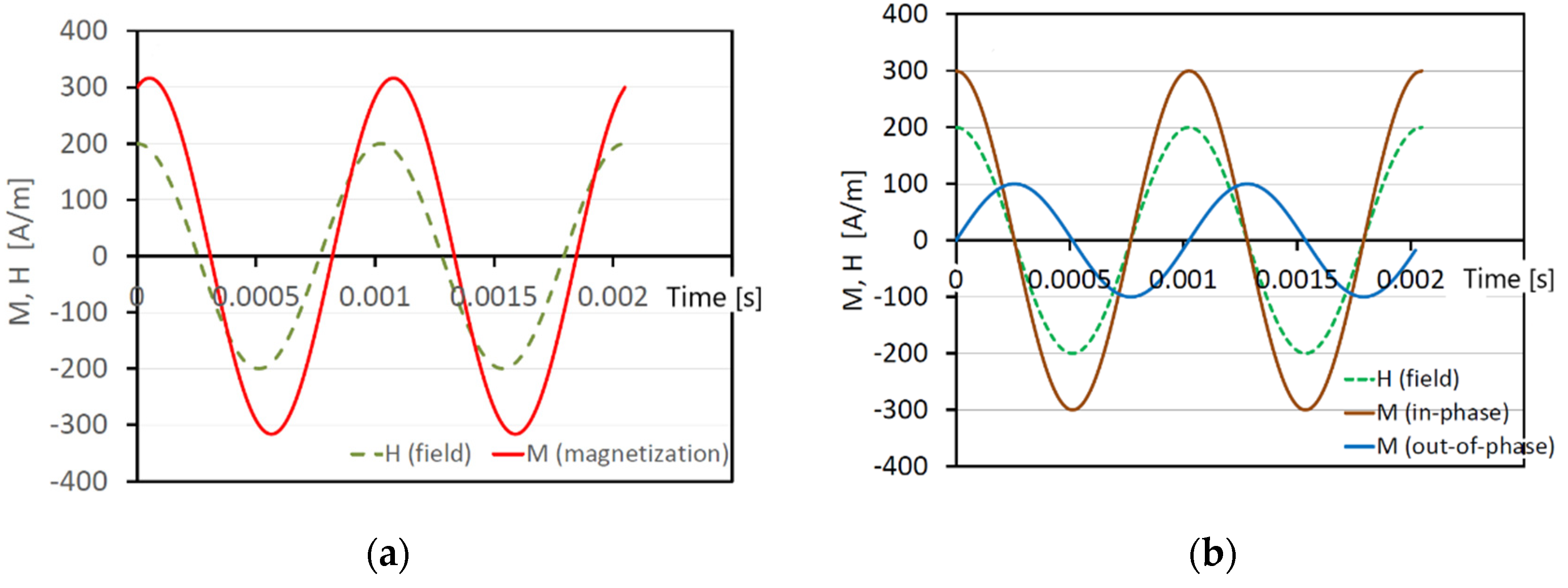
2.1. Physical Principles of Out-Of-Phase Magnetic Susceptibility

In measuring magnetic susceptibility in a low alternating magnetic field, the measured specimen is usually magnetized by a weak field (in the order of hundreds A/m) sinusoidally varying in time:

H(t)= H_o cos(ωt)

(1)

where H_o is amplitude, ω is angular frequency, and t is time, and the magnetic response is measured, most conveniently represented by magnetization. In diamagnetic, paramagnetic, and many ferromagnetic minerals, the magnetization also varies sinusoidally; because it is in phase with the applied field and the magnetization-to-field ratio, then it maintains a constant value that represents the susceptibility. In some ferromagnetic and/or electrically conductive minerals, however, the magnetization is not in phase with the applied field, but it lags behind the field (Figure 1a) and may therefore formally resolve into in-phase and out-of-phase components (Figure 1b). The ipMS and opMS are defined correspondingly:

M(t) = H_o k′cos(ωt) + H_o k″sin(ωt)

(2)

where M(t) is magnetization, H_o is amplitude of the magnetizing field, ω is angular frequency, t is time, k′ and k″ are ipMS and opMS components, respectively, related as tan δ = k″/k′, with δ being referred to as the phase angle or simply phase.

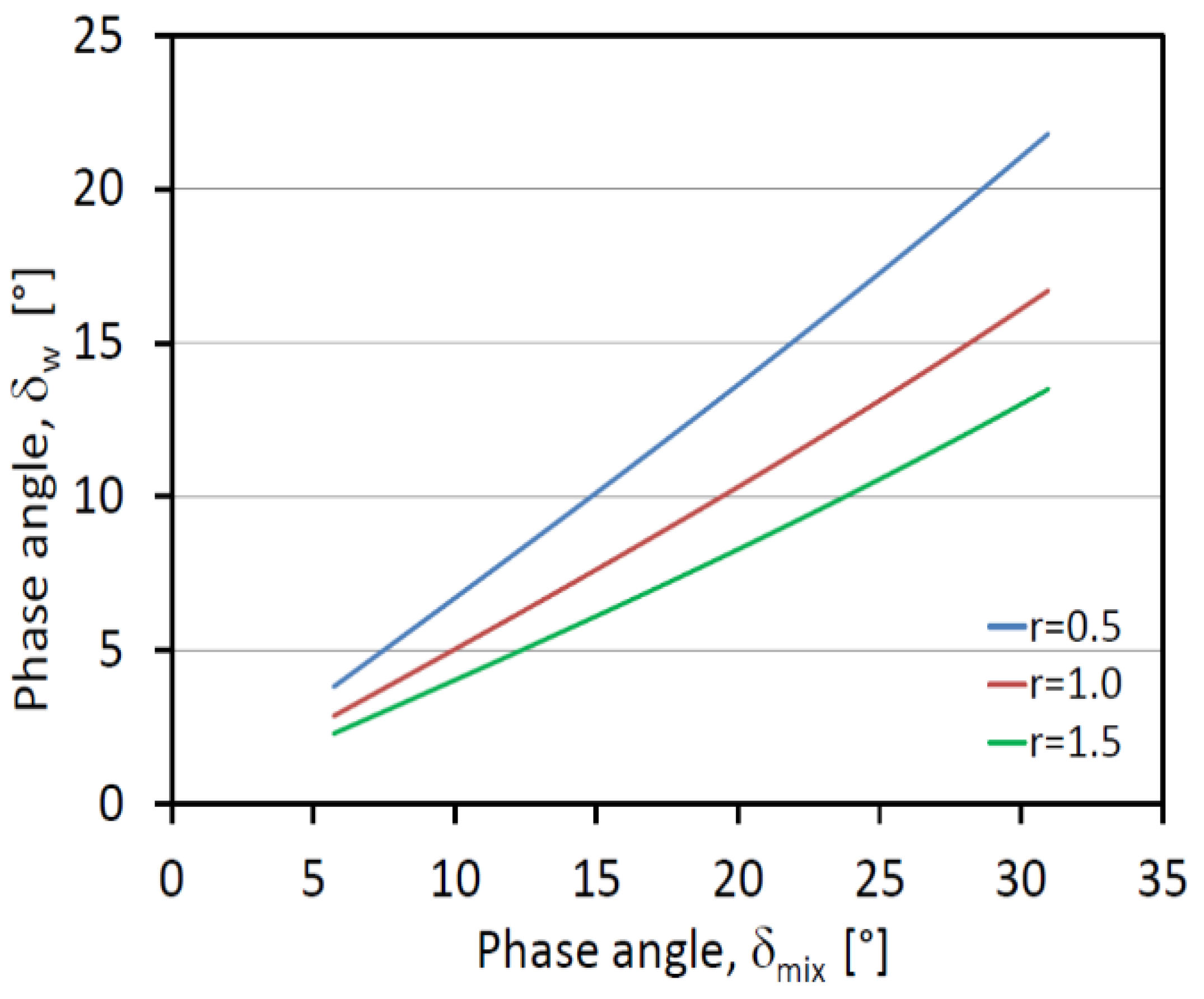
2.2. Effect of Mineral Fractions with Exclusive In-Phase Response on the Whole Rock Phase Angle

In general, rocks consist of dia-, para-, and ferromagnetic sensu lato minerals. The whole rock susceptibility can then be described, assuming the minerals mutually not interact magnetically, by the following model [6,7,8]:

k_w = c_dk_d + c_pk_p + c_fk_f = K_d + K_p + K_f

(3)

where k_w is the whole rock susceptibility, k_d, k_p, k_f are susceptibilities of dia-, para-, and ferromagnetic fractions, respectively, and c_d, c_p, c_f are the respective percentages; K_d, K_p, K_f are called the respective contribution susceptibilities. Analogously, we can introduce another susceptibility resolution:

k_w = K_ip + K_mix

(4)

where K_ip is the contribution susceptibility of the mineral fraction that possesses only the in-phase response (its opMS is zero) and K_mix is the contribution susceptibility of the mineral fraction whose opMS is non-zero. Re-writing this equation in terms of in-phase and out-of-phase contribution susceptibilities yields:

k′_w = K_ip + K′_mix

k″_w = K″_mix

(5)

tan δ_w = k″_w/k′_w = tan δ_mix/(1 + r)

where tan δ_mix = K″_mix/K′_mix and r = K_ip/K′_mix. It is obvious that while the whole rock in-phase contribution susceptibility is controlled by all mineral fractions present in the rock, the out-of-phase contribution susceptibility is solely controlled by the fraction whose opMS is non-zero. However, the phase angle is affected by both the fractions present. Figure 2 shows the tan δ_w vs. tan δ_mix plot for several r ratios, indicating that the increasing amount of the fraction with only in-phase response results in decreasing the whole rock phase angle.

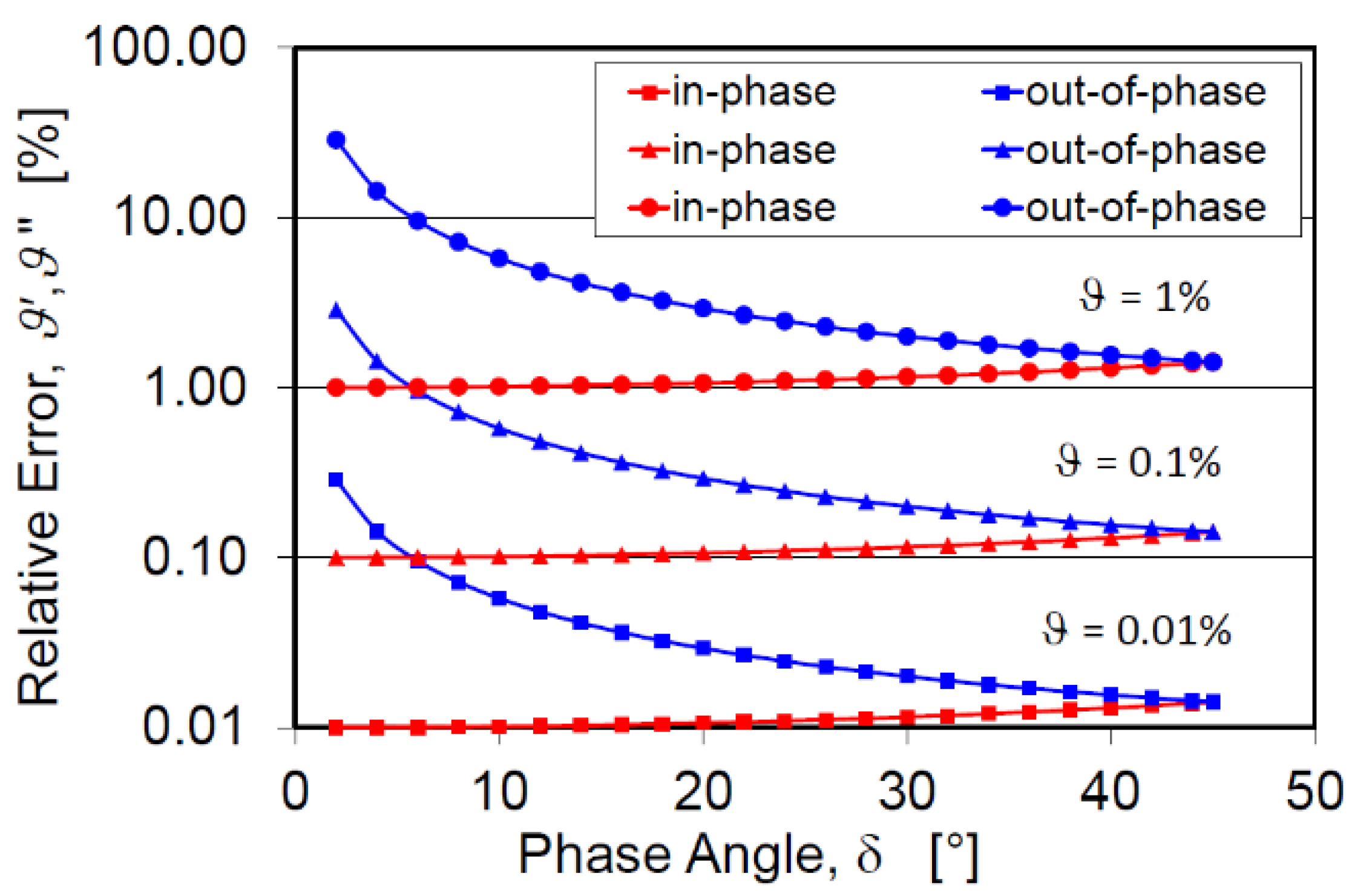
2.3. Accuracy of opAMS Determination

The principle of the AMS determination lies in measuring the susceptibility in several (at least six) independent directions and subsequent fitting the second rank symmetric susceptibility tensor to these data using the least squares method. The accuracy in determination of the AMS can be characterized by the errors in determining the principal susceptibilities and principal directions. Hrouda and Pokorný [10,11] showed that there is a close relationship between measurement precision of directional susceptibilities and the accuracy of the determination of the AMS.

In all inductive bridges, the overall magnetic response is primarily measured, which is subsequently resolved into the in-phase and out-of-phase components presented in terms of susceptibility. Hrouda et al. [1] showed that the relative error in measuring directional susceptibility varies between 0.1% and 0.01% in the MFK1 and KLY5 Kappabridges, tending to slightly decrease with increasing field.

It is intuitively considered that in rocks having a small phase angle, the measuring error in ipMS will be very low, whereas that in opMS will be very high. On contrary, in materials with large phase angle (e.g., conductive ores, graphites) the measuring error in ipMS will be high, whereas that in opMS will be low. The situation in rocks with phase angles ranging from 0° to 45° is illustrated in Figure 3, which shows the relative errors in ipMS (ϑ′) and opMS (ϑ″) according to the phase angle and relative error in measuring directional susceptibility (ϑ). It is evident that the ipMS relative error, ϑ′, increases slowly from ϑ′ = ϑ to ϑ′ = √(2ϑ) for δ = 45°. At δ = 45° it holds ϑ″ = ϑ′. With decreasing phase angle, ϑ″ initially increases slowly and for δ < 10° dramatically, reaching extremely high values for δ near zero. The relative error in opMS is almost always clearly higher than that in ipMS.

In the KLY5 Kappabridge, the opAMS is measured simultaneously with ipAMS and calculated, even in the case when the phase angle is small and the calculated anisotropy is insignificant from the statistical point of view. For this reason, it is highly recommended to inspect the results of the statistical tests of each specimen provided by the instrument-control software. The basic statistical test is the F-test, which serves to verify whether the differences between the principal susceptibilities are large enough compared to measuring errors for the specimen to be regarded as anisotropic. The same test is used to find out whether the AMS ellipsoid is statistically rotational or triaxial. In addition, the errors in determining the principal susceptibilities and the confidence angles about the principal directions are presented (for details see [12]). Then, the specimens whose opAMS is statistically insignificant should be excluded from further processing. The problem is that the decision about the precision sufficiency is multi-criteria and cannot be simply algorithmized. Therefore, the decision is not included in the measuring software.

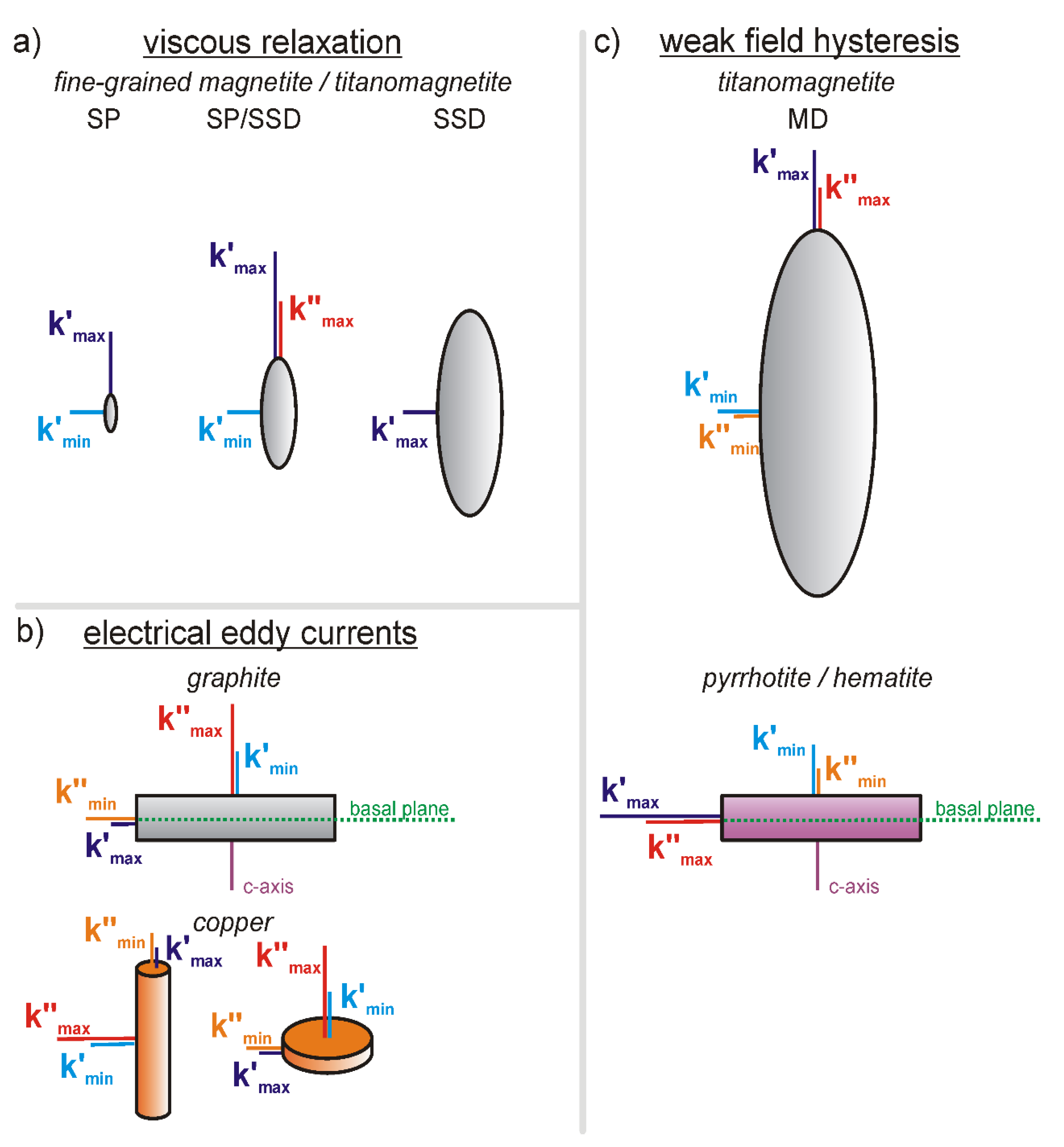
3. Physical Mechanisms That Produce Out-Of-Phase Susceptibility

There are three major physical mechanisms that produce the opMS [13]:

(1)

viscous relaxation,

(2)

electrical eddy currents (induced by AC field in conductive materials),

(3)

weak field hysteresis (non-linear and irreversible dependence of M on H).

Mechanism (1) is typical of ultrafine magnetic particles (usually magnetite and maghemite) that are between the blocked and unblocked states at superparamagnetic (SP)/stable single domain (SSD) boundary. Mechanism (2) is typical of minerals that are at least moderately conductive electrically. Mechanism (3) is typical of the minerals that show a wide hysteresis loop (titanomagnetite, pyrrhotite, hematite) [13].

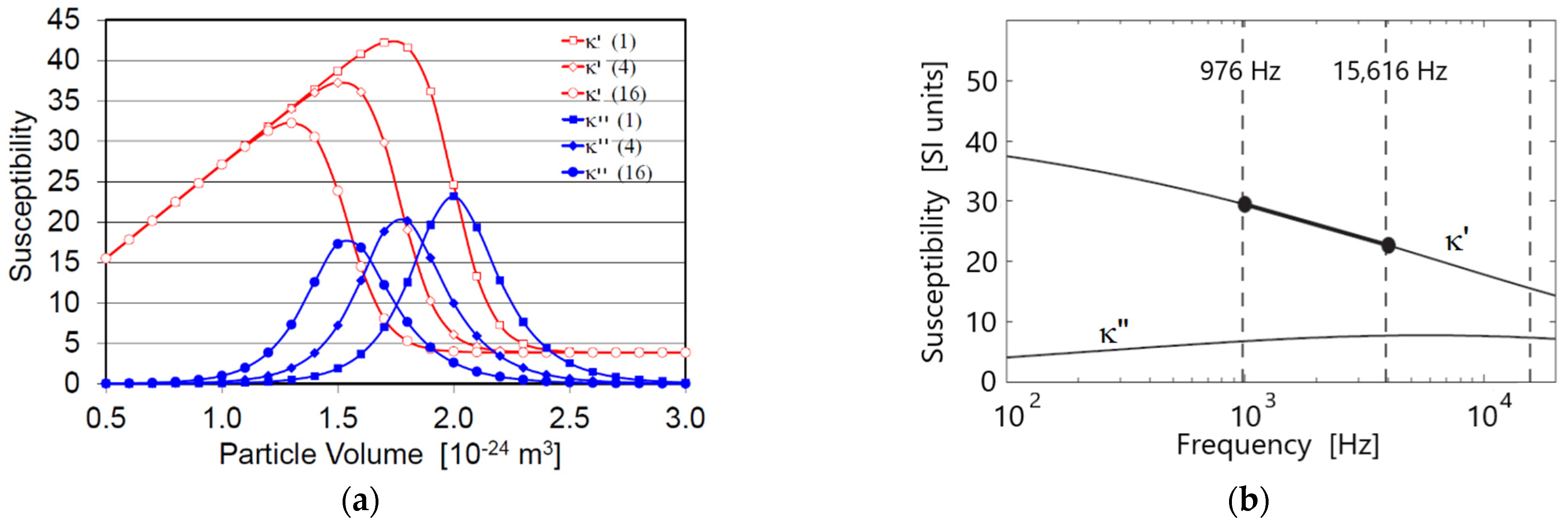
3.1. Viscous Relaxation

The susceptibility of viscous magnetic particles that are between the blocked and unblocked states at the SP/SSD boundary resolves into a component that is in-phase with applied field (κ′) and a component that is out-of-phase (κ″). It can be described by the formula introduced by Néel [14] and transcribed by Egli [15], using terms of linear dynamic susceptibility, κ = κ′ − iκ″, as follows:

$${\kappa }_{sp/sd}={\kappa }_{sd}\left[\frac{\beta }{1+i{\tau }_o\omega e^{\beta }}+1\right]$$

(6)

where κ_sd = 2M_s/3H_k, β = K_aV/k_BT and ω = 2πf; M_s is saturation magnetization, H_k is microscopic coercivity related to macroscopic coercivity (H_c) as H_k = 2.09H_c [16], K_a is the aniso- tropy constant, V is the particle volume, k_B is the Boltzmann constant, T is the absolute temperature, τ_o ≈ 10^–10 s is a time constant, and f is the operating frequency.

Figure 4a shows the susceptibility vs. particle volume plot for three frequencies (corresponding to those of the MFK-1 Kappabridge) for magnetite (K_a = 2.5 × 10⁴ J/m³, see [17]). Initially, ipMS almost linearly increases with grain size, while the opMS is effectively zero. After reaching the maximum value, the ipMS acutely decreases to SSD susceptibilities. The peak ipMS decreases with increasing frequency and shifts towards the smaller particle volumes. The opMS increases, creating a bell-like curve and subsequently dropping to effectively zero. The peak opMS also decreases with increasing frequency and shifts towards the smaller particle volumes. Consequently, whereas the ipMS is non-zero in the entire interval of particle volumes considered and therefore affected by the particles of relatively wide grain-size interval, the opMS is non-zero and dominantly affected by the particles of much narrower interval.

It follows from Equation (6) and Figure 4a that both the ipMS and opMS of individual particles are low-field independent and frequency dependent. However, magnetic particles in rocks are never of the same volume but generally show a wide distribution. Figure 4b shows variations in ipMS and opMS with logarithm of the frequency for a lognormal distribution of grain volumes (with μ = −23.7 and σ = 0.1 being mean and standard deviation, respectively, of the logarithms of the grain volume). The ipMS curve relatively closely resembles a negatively sloped straight line in the frequency range of the MFK and KLY-5 Kappabridges, while the opMS curve is only very weakly sloped positively, in the first approximation, passing roughly parallel to the abscissa. Mathematical modeling of phase angle (δ) distribution vs. particle volume, considering both narrow (σ = 0.3) and wide (σ = 0.8) distributions of grain volumes, showed that the phase angle is mostly less than 20° [9].

Figure 4c,d show the field and frequency dependence of opMS and ipMS in ultrafine magnetic particles from a ferromagnetic liquid (mixture of ultrafine magnetite particles in mineral oil as described in [18]. Both susceptibilities change with field only slightly, but with frequency considerably. In accordance with theory, the opMS increases with frequency, whereas the ipMS decreases.

The anisotropic properties of ultrafine magnetic particles (magnetite/titanomagnetite ranging from SP to SSD in state) were investigated in [19] through calculating the ipMS and opMS parallel and perpendicular to the particle shape; they are schematically summarized in Figure 5a. In SP particles, the ipMS along the particle long dimension is much larger than that along the particle short dimension. In SSD particles, the ipMS along the particle long dimension is zero and along the short dimension it is non-zero. The opMS parallel to the particle short dimension is effectively zero in the entire particle size range considered and the opMS along the long dimension is non-zero only in the viscous state (SP/SSD). Consequently, the maximum opMS is parallel to the long dimension of the viscous particle and, therefore, the opAMS fabric is conformable to the shape fabric of magnetite/titanomagnetite. The degrees of both ipAMS and opAMS of a particle are considerably variable depending on the particle size. It is worth noting that the SP/SSD interval is located at considerably larger grain sizes in maghemite and titanomagnetite than in magnetite [17].

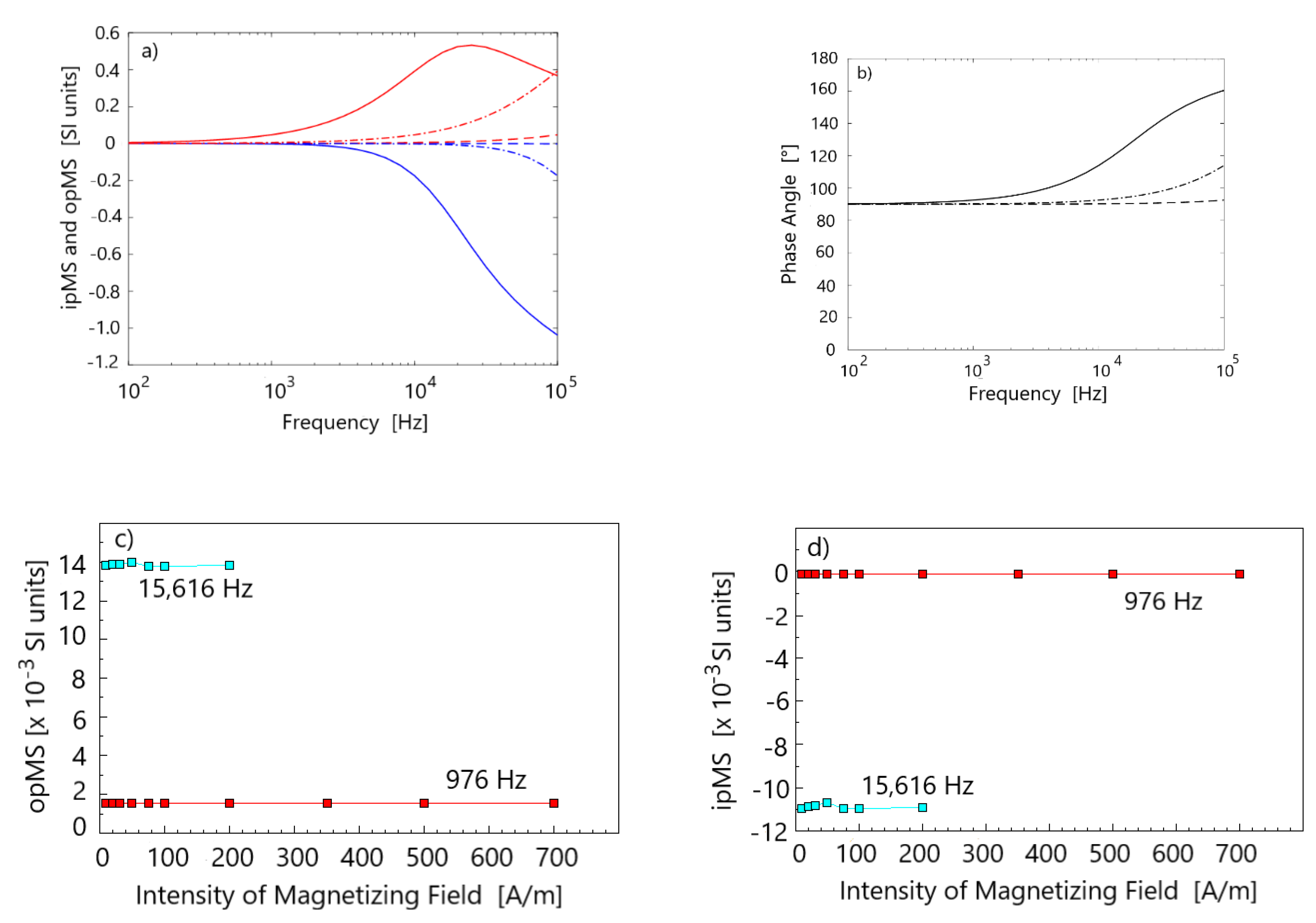
3.2. Electrical Eddy Currents

The alternating driving magnetic field in the measuring instrument induces electric current in conductive materials, which is out-of-phase with the driving field. This current in turn produces a secondary magnetic field, which is also out-of-phase with the driving field. Complications arise because the time-varying secondary magnetic fields also generate currents and thus produce tertiary time-varying magnetic fields. Moreover, the eddy currents dissipate energy, and the external field variations are consequently attenuated in the material, with a scale length (“skin depth″) related to resistivity and permeability of the material, and the frequency of the applied field, and response is thus a strong function of the size and shape of a conductive body (e.g., [13]).

Magnetic susceptibility due to eddy currents follows from Maxwell equations. Analytical solutions of Maxwell equations for eddy currents are known for a sphere [20,21] and infinite cylinder [21,22]. For bodies having other shapes, a closed form formula does not exist and numerical solutions of Maxwell equations must be used (e.g., [23,24,25]).

Magnetic susceptibility of an isotropic conducting sphere can be expressed:

$$k^{\prime }+i{k}^{″}=\frac{3\mu (sinh\alpha -\alpha cosh\alpha )+3/2{\mu }_o\left(sinh\alpha -\alpha cosh\alpha +{\alpha }^{2}sinh\alpha \right)}{\mu \left(sinh\alpha -\alpha cosh\alpha \right)-{\mu }_o\left(sinh\alpha -\alpha cosh\alpha +{\alpha }^{2}sinh\alpha \right)}$$

(7)

where $\alpha =r\surd \left(i\sigma \mu \omega \right)$ and r, σ, and μ are the sphere′s radius, conductivity, and permeability, respectively, μ₀ is permeability of surrounding medium (air or rather matrix, in the context of measurement of magnetic susceptibility), and ω is angular frequency of the applied field.

Figure 6a shows the ipMS and opMS of a sphere with zero DC susceptibility as a function of operating frequency (f), sphere radius (r), and electrical conductivity (σ). In a sphere with r = 1 mm and σ = 6 × 10⁷ S/m, ipMS is only slightly negative at frequencies less than 2 × 10³ Hz; thereafter, it decreases substantially with increasing frequency. opMS is positive and increases with increasing frequency until 10.5 kHz, and then decreases but remains positive. In smaller and less conductive spheres, the basic trends are retained, but are less expressive and shifted to higher frequencies. Figure 6b shows the phase angle (δ) of the same sphere. At low frequencies (f~100 Hz), the phase angle δ = 90°, then increases with increasing frequency, reaching δ = 180° at very high frequencies when eddy currents are confined to a thin surface layer of the sphere and create a magnetic moment that is antiparallel to the applied field.

Figure 6c,d show the variation of both opMS and ipMS with magnetizing field and with frequency for copper, whose opMS is no doubt due to eddy currents. It is obvious that both the opMS and ipMS are field independent, but strongly frequency dependent, in agreement with theory.

The anisotropic properties of materials whose opMS is due to eddy currents were investigated using the examples of graphite single crystals and workshop-made copper cylinders [25,26]. In graphite, whose DC susceptibility and ipMS are negative, the opMS is positive and an order-of-magnitude larger along the c-axis than along the basal plane (Figure 5b). In copper cylinders, the DC susceptibility and ipMS are also negative. In elongated cylinders the opMS is lower along the cylinder axis compared to the perpendicular plane. In flattened cylinders, the inverse relationship holds. If opAMS is used to investigate preferred orientation of graphite in rocks, one has to realize that it would be the maximum opMS that would be perpendicular to the rock schistosity provided that graphite grains are parallel to the schistosity with their basal planes.

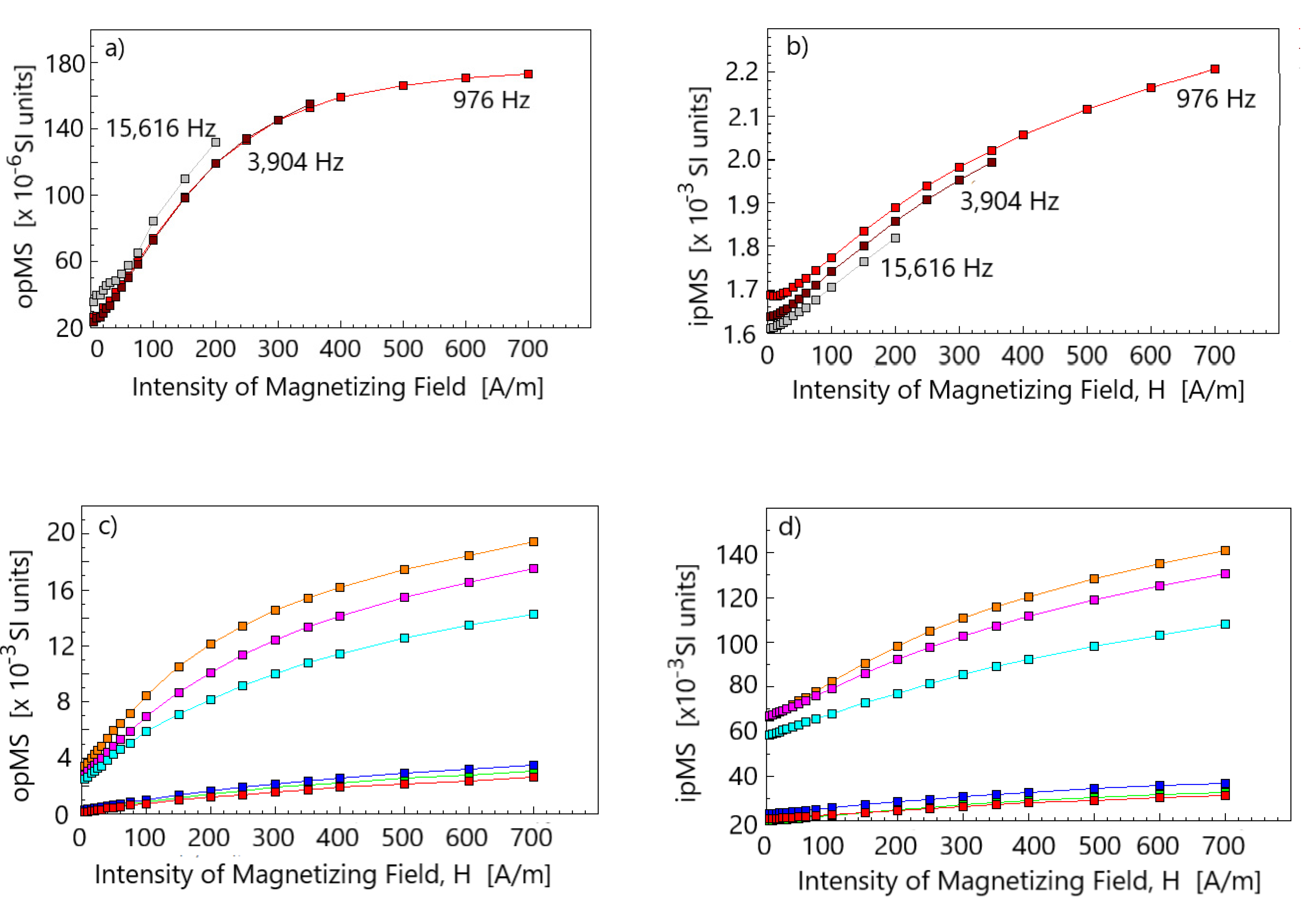
3.3. Weak Field Hysteresis

During susceptibility measurement in low alternating magnetic field, the specimen is magnetized along a minor hysteresis loop. The magnetization lags behind the field due to the irreversible character of the process and the susceptibility may therefore be resolved into the in-phase and out-of-phase components. Quantitative description of this process exists for multi-domain (MD) materials measured in such low fields (less than coercivity) in which the empirical Rayleigh Law is valid:

M = κH + αH²

(8)

where M is magnetization, H is intensity of the magnetizing field, κ is initial susceptibility, and α is the Rayleigh coefficient. The ipMS and opMS are:

k′ = κ + αH,

(9)

k″ = 4αH/3π,

(10)

where H is amplitude of the field intensity (e.g., [13,27]). It follows from the above equations that the relationships between ipMS or opMS and the magnetizing field are represented by straight lines. Although the slope of the relationship ipMS vs. field intensity straight line defines the Rayleigh coefficient, α, that of the opMS line is 4/3π times smaller. The straight lines of ipMS show a non-zero intercept equaling the initial susceptibility, κ, but the opMS line passes through the origin. Frequency dependence of susceptibility as affected by grain shape is discussed by Newell [28]).

Figure 7a,b show the variation of both opMS and ipMS with the magnetizing field in high-Ti titanomagnetite (Curie temperature less than 100 °C) using the example of a magnetic fraction extracted from a volcanic dyke. Both the susceptibilities show strong field dependence, but very weak (almost zero) frequency dependence. Analogous curves for pure magnetite are not presented because pure magnetite possesses very low, virtually zero opMS. Figure 7c,d show the variation of both opMS and ipMS with the magnetizing field for pyrrhotite bearing rocks. Both opMS and ipMS increase with the field relatively rapidly in very low fields (typically H < 100 A/m), becoming curved in stronger fields. The opMS vs. field curves in Figure 7a,c do not project directly to the origin, which contradicts Equation (10). The minimum field intensity in KLY-5 Kappabridge is 5 A/m; therefore, for Equation (10) to be valid, the opMS vs. field curves must be strongly curved in the fields <5 A/m.

The anisotropic properties of opMS in titanomagnetite, which possesses shape anisotropy, were investigated by Hrouda et al. [29]). It was found that the maximum opMS and ipMS are parallel to the longest dimension of the MD particle, whereas the minimum susceptibilities are parallel to the shortest dimension (Figure 5c). Therefore, the opAMS is conformable to the particle shape. In pyrrhotite and hematite, the maximum opMS and ipMS are parallel to the basal plane, whereas the minimum opMS and ipMS are parallel to the c-axis [26,30].

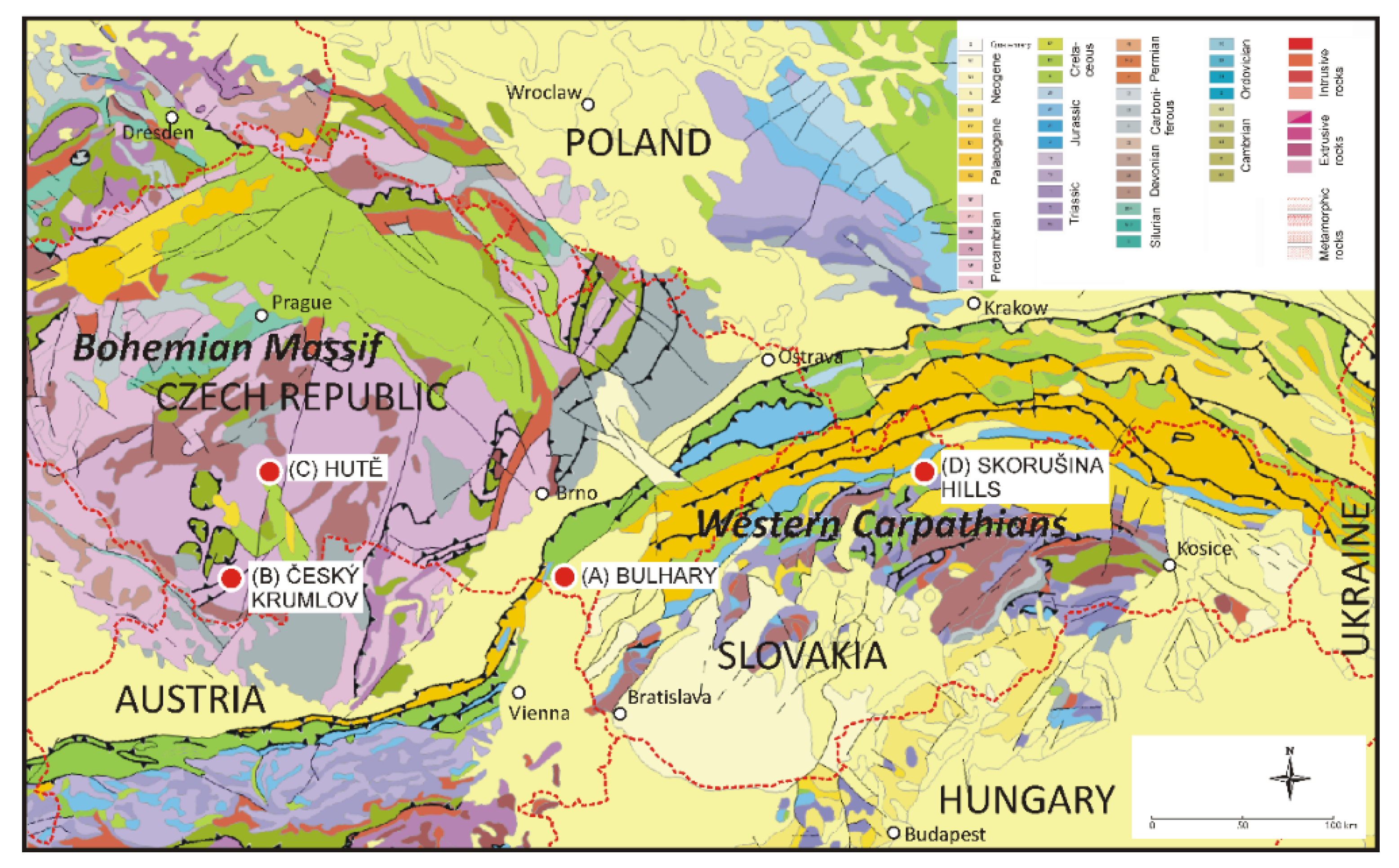
4. Examples of Geological Applications

In this section, examples are shown of the application of the opAMS in solving various geological problems. They come from the Bohemian Massif and the Western Carpathians (Figure 8).

4.1. Instrumentation and Data Processing

The ipMS and opMS and their variations with the magnetizing field, and their anisotropies presented in this paper, were measured with the KLY5-A Kappabridge [31,32] in the field having a 400 A/m peak at the operating frequency 1220 Hz at room temperature. Computation of the opAMS was exactly the same as that for computation of the ipAMS and both the anisotropies were determined simultaneously. The ipMS and opMS variations with operating frequency were investigated at the frequencies 976, 3904, and 15,616 Hz in the driving field of 200 A/m using the MFK1-FA Kappabridge [33]. The susceptibility variation with temperature was measured on coarsely powdered pilot specimens using the CS-L Cryostat, CS-4 Furnace [34], and the MFK1-FA Kappabridge. The Curie temperatures were determined using the Petrovský and Kapička [35] method based on searching for the beginning of the paramagnetic hyperbola just at the Curie temperature.

It is usual to represent the susceptibility tensor by convenient parameters derived from principal susceptibilities (e.g., [36,37]), for instance:

K_m = (K₁+K₂+ K₃)/3

(11)

P = K₁/K₃

(12)

T = (2η₂ − η₁ − η₃)/(η₁ − η₃) = 2lnF/lnP − 1

(13)

where K₁ ≥ K₂ ≥ K₃ are the principal susceptibilities, η₁ = lnK₁, η₂ = lnK₂, η₃ = lnK₃, and F = K₂/K₃. The parameter K_m is called the mean susceptibility and characterizes the qualitative and quantitative content of magnetic minerals in a rock. The parameter P, called the degree of AMS, indicates the intensity of the preferred orientation of magnetic minerals in a rock. The parameter T, called the shape parameter, characterizes the symmetry or shape of the AMS ellipsoid. If 0 < T < +1, the AMS ellipsoid is oblate (the magnetic fabric is planar); T = +1 means that the AMS ellipsoid is rotationally symmetric (uniaxial oblate). If −1 < T < 0, the AMS ellipsoid is prolate (the magnetic fabric is linear); T = −1 means that the AMS ellipsoid is uniaxial prolate.

In order to obtain a statistical evaluation of the AMS tensors, the ANISOFT program [38,39] can be used, which enables a complete statistical evaluation of a group of specimens to be carried out; the mean principal directions are determined in addition to the confidence areas around them at the likelihood level of 95%.

4.2. Fabric of Ultrafine Magnetic Particles in Loess/Palaeosol Sequences—Viscous Relaxation

Viscous relaxation is often active in loess/palaeosol sequences, in which ultrafine magnetic particles are created during pedogenesis. We present the opAMS of such loess/palaeosols sampled at the Bulhary section in the Dyje River Valley (Figure 8), Southern Moravia [19]. The section exposes Eemian Interglacial brown soil developed on top of Saalian loess. The interglacial soil is covered with early glacial chernozem overlain by last glacial loess.

The ipMS is in the order of 10⁻⁴, and the opMS is about an order lower, with both showing virtually no variations with the measuring field. The ipMS possesses relatively high frequency dependence; ipMS at 15,616 Hz is up to 10% lower than at 976 Hz. In addition, the percentage loss of susceptibility between 976 and 15,616 Hz increases with ipMS (Figure 9a). This increase can be traditionally (since [40]) interpreted as resulting from creation of new SP particles in soil layers during pedogenesis. Consequently, the opMS is evidently due to viscous relaxation and indicates preferably oriented viscous particles in the transition between SP and SSD states (cf. [13]). The ipAMS, by comparison, is controlled not only by these grains, by also by the MD, SSD, and SP grains, and by paramagnetic grains.

The degree of opAMS is mostly higher than that of ipAMS (Figure 9b). This phenomenon may be explained by the grain degree of opAMS being an order-of-magnitude higher in ultrafine magnetically viscous particles than the degree of ipAMS in MD particles, and also by a possible effect of paramagnetic minerals on the ipMS (for details see Section 2.2). The shape parameters of opAMS are more scattered and less oblate than those of ipAMS (Figure 9b). Both the opAMS and ipAMS foliation poles create roughly vertical clusters, whereas the respective lineations are widely scattered in the horizontal plane with the mean direction being NW–SE to NNW–SSE (Figure 9c,d). The cluster of opAMS foliation poles is elliptic and that of the ipAMS poles is roughly concentric.

The magnetic lineations in wind-blown sediments, such as loess, which have not been re-deposited or deformed ductilely, are parallel to the wind (see [41] for a summary). This interpretation is justified provided that the magnetic foliation is more or less horizontal. However, the opAMS foliations show at least partial fan-like orientation of magnetically viscous particles, which may have slightly rotated in an oriented way during their deposition or during their post-depositional history.

4.3. Preferred Orientation of Graphite in Graphite-Bearing Rocks and Graphite Ores—Eddy Currents

Single crystals of graphite are diamagnetic and show magnetocrystalline anisotropy of DC susceptibility [42]. In addition, graphite is moderately electrically conducting with strong anisotropy of electrical conductivity [43]). The AC susceptibility exhibits a weak and negative in-phase component and a relatively strong out-of-phase component, likely due to electrical eddy currents. Consequently, if graphite crystals are preferentially oriented by their crystal lattices (LPO) in a rock, one would expect a correspondingly strong AMS. However, the standard AMS (i.e., ipAMS), reflects not only the LPO of graphite, but also the preferred orientation of paramagnetic and ferromagnetic admixtures. On the other hand, the opAMS should indicate the LPO of graphite, free of the effects of non-conductive paramagnetic and ferromagnetic minerals. We present here the results from metamorphic graphite ores sampled in a former graphite mine (Městský vrch locality near Český Krumlov town) located in the Moldanubian Zone in Southern Bohemia (Figure 8). For more details see [26].

The opMS is low, mostly less than 8 × 10^–5, compared to the ipMS, which is an order-of-magnitude higher. Both opMS and ipMS are independent with respect to the intensity of the magnetizing field (Figure 10a,b). The ipMS shows virtually no dependence on the operating frequency, whereas the opMS is strongly frequency dependent (not shown in the figure).

Regarding the temperature variation of susceptibility, the ipMS conspicuously increases in the vicinity of −155 °C, which may represent the Verwey transition typical of magnetite (Figure 10c). However, the peaked curve shape at the Verwey transition is atypical for magnetite alone. Its existence can be explained as the superposition of a Verwey transition together with a paramagnetic hyperbola (1/T). During specimen heating, the ipMS remains more or less constant up to 280 °C or even to 450 °C, and then it increases substantially and subsequently decreases acutely at about 580 °C (Figure 10d). The cooling ipMS vs. T curves (not presented for scale reasons) show order-of-magnitude higher susceptibilities than heating curves. These ipMS variations can be interpreted in terms of neo-formation of Fe-Ti oxides (including magnetite) due to alteration during heating. The opAMS is carried by graphite.

The degree of ipAMS is weak to moderate, with fabrics being neutral to moderately planar (Figure 11b). K₁ and K₃ axes are relatively tightly grouped. The ipAMS foliations dip moderately, being similarly oriented as the metamorphic schistosity (Figure 11d). The ipAMS lineations plunge and lie near the mesoscopic lineation. The degree of opAMS is very high and the opAMS fabric ranges from neutral to linear (Figure 11a). K₁ and K₃ axes are switched between ipAMS and opAMS (Figure 11c).

4.4. Preferred Orientation of Pyrrhotite in Eclogite with Complex Magnetic Mineralogy—Weak Field Hysteresis

Eclogites are found as numerous bodies within the Moldanubian Zone of the Bohemian Massif. We present results from a body on the locality of Hutě in central Bohemia (Figure 7). In eclogite from this locality, both the opMS and ipMS increase with magnetizing field relatively intensely (Figure 12a,b). The heating susceptibility vs. temperature curve is characterized by paramagnetic hyperbola at low temperature; by an acute susceptibility decrease in the temperature interval between 320 and 330 °C, which corresponds to the Curie temperature of pyrrhotite; and by a slow susceptibility increase up to 470 °C, followed by a slow decrease above 470 °C and a relatively rapid decrease at 590 °C, which corresponds to magnetite or weakly oxidized magnetite (Figure 12c). The paramagnetic contribution to the room temperature rock susceptibility determined through the resolution of the susceptibility vs. temperature curve into the paramagnetic hyperbola and ferromagnetic straight line parallel to the abscissa using the method by Hrouda [44] is about 75%. The decrease in susceptibility between 243 and 365 °C (due to the Curie temperature of pyrrhotite) is about 50% and the decrease between 365 and 615 °C (due to the Curie temperature of magnetite) is 65%. Summarizing the above data in very rough terms, we can say that the room temperature susceptibility consists of 75% paramagnetic contribution, 18% pyrrhotite contribution, and 7% magnetite contribution. Hence, the susceptibility and AMS carriers are complex and comprise paramagnetic mafic silicates, pyrrhotite, and magnetite.

The degree of ipAMS is relatively high and scattered moderately and the ipAMS ellipsoids are strongly prolate (Figure 13a). The ipAMS lineations create a narrow cluster and the ipAMS foliation poles create an elliptic cluster whose mean direction is near the poles of mesoscopic foliation defined as compositional banding (Figure 13b). The degree opAMS is high and the opAMS ellipsoids are strongly prolate (Figure 13a). The opAMS lineations create a narrow cluster, which is virtually identical with the cluster of the ipAMS lineations, and the opAMS foliation poles create an elliptic cluster resembling the cluster of the ipAMS foliation poles (Figure 13b). Consequently, the whole-rock magnetic fabric and the pyrrhotite magnetic sub-fabric are highly co-axial.

It is highly likely that both the ipAMS and opAMS fabrics originated during the same process. Petrological investigations revealed that the eclogites of this locality underwent only minimum post-genetic compositional changes (Prof. S.W. Faryad, personal communication). In addition, they show relatively high bulk density and moderate mean susceptibility carried predominantly by paramagnetic mafic silicates, subordinately by pyrrhotite and very sub-ordinately by magnetite. All these findings together with the virtual coaxiality of both magnetic foliations to the metamorphic compositional banding make us believe that the process forming both the whole-rock ipAMS fabric and the pyrrhotite opAMS fabric was the creation of the eclogites in the uppermost mantle and/or lowermost crust.

4.5. Ferromagnetic Mineral Fabric Masked by Paramagnetic Fraction in Whole-Rock AMS in Sedimentary Rocks

Sedimentary rocks in the Intra-Carpathian Palaeogene of the Western Carpathians possess a range in magnetic fabrics from almost pure sedimentary to composite tectonic plus sedimentary, although they lack visible cleavage [45]. Their ipMS is dominantly carried by paramagnetic minerals (clays), and the opMS, which is about two orders lower, is carried by slightly non-stoichiometric MD magnetite [46]. We present results from a part of the Intra-Carpathian Palaeogene, the Skorušina Hills, whose sandstone magnetic fabrics represent a gradual transition from almost purely sedimentary in origin to those that underwent a deformational overprint. The opAMS and ipAMS fabrics are complemented by the anisotropy of magnetic remanence (AMR) fabric, which indicates similar but not fully identical ferromagnetic mineral fabric. Unlike the paper [46], in which ipAMS and AMR of all specimens investigated were present, we present all three anisotropies of only those specimens whose opAMS is statistically significant.

The ipAMS foliations are mostly parallel to the bedding, which, at first sight, is indicative of sedimentary fabric. This is well seen in the tilt corrected coordinates, where the ipAMS foliation poles of the most specimens are concentrated near the center of the projection net (representing the bedding pole) and the ipAMS lineations are mostly oriented NE–SW (Figure 14a). The opAMS foliation poles create an imperfect, NW–SE oriented girdle, whereas the opAMS lineations mostly trend NW–SE, perpendicular to most ipAMS lineations (Figure 14b). The AMR foliation poles create a relatively wide cluster near the center of the projection net and the AMR lineations show mostly NW–SE orientations (Figure 14c).

As revealed by Hrouda and Potfaj [45], Pešková et al. [46] and Nemčok [47], the palaeostress field in the area investigated was controlled by interaction between the Apulian and European plates or, in other words, between the Adria microplate and the European Platform. The rocks investigated were deformed through the convergence of the European and Apulian plates and tectonic escape of the Central Western Carpathians through complex strike-slip movement along the Klippen Belt.

The NE–SW oriented ipAMS lineations are due to the weak fan-like orientation of platy clay minerals whose intersections define the magnetic lineation. The fabric is interpreted as indicating lateral NW–SE shortening combined with simple shear in the same direction, probably associated with convergence movements of the European and Apulian plates [45]. The opAMS lineations, mostly oriented NW–SE, i.e., parallel to the girdle in opAMS foliation poles, are due to the cluster orientation of elongated grains of impure magnetite. The difference in the orientations of ipAMS and opAMS lineations are interpreted in terms of higher sensitivity of ferromagnetic minerals to deformation than that of the paramagnetic clay minerals.

The AMR foliation poles create a relatively wide cluster near the center of the projection net and the AMR lineations show mostly a NW–SE orientation. The difference in the orientations of opAMS and AMR foliations can be explained in such a way that the AMR indicates all the ferromagnetic minerals that can be easily magnetized anhysteretically and subsequently demagnetized before changing the magnetizing direction, whereas the opAMS indicate only those ferromagnetic minerals that show non-zero opMS.

5. Discussion

The AMS is widely used in the investigation of the preferred orientation of magnetic minerals in rocks. In general, it is affected by all minerals present in rocks. As the individual minerals or their fractions may show different sensitivities to various geological processes, it is desirable to investigate the magnetic sub-fabrics of individual minerals or their fractions. The opMS, on the other hand, is effectively zero in most minerals, being non-zero in only some minerals; for example, in magnetically viscous ultrafine grains of magnetite or maghemite, in weakly magnetic (even diamagnetic) but at least moderately conductive electrically minerals such as graphite, and in ferromagnetic sensu lato minerals showing a wide hysteresis loop (e.g., pyrrhotite, hematite, titanomagnetite). The opAMS of rocks containing these minerals may serve as a tool for the direct determination of the magnetic sub-fabrics of these minerals. This is a great advantage because the opAMS is measured simultaneously with the ipAMS.

Unfortunately, there are some limitations in the wide use of the method, consisting in measurement accuracy problems. Namely, the opAMS is not measured directly, but what is measured is the overall response, which is subsequently resolved into the ipMS and opMS components. For this reason, the precision in the opAMS determination decreases relatively rapidly with decreasing phase angle (see Figure 3). As the opMS is usually at least an order of magnitude lower than the ipMS, the error in determination of ipMS resembles that of complex susceptibility, whereas the error in determination of the opMS may be considerably higher, mainly in specimens with a very low phase angle (for details see [1]).

In order to avoid problems possibly arising from all the above effects, it is highly recommended to inspect the results of the statistical tests of each specimen provided by the SAFYR program (version 7, M. Chadima, Brno, Czech Republic, www.agico.com (accessed on 13 February 2022)). The basic statistical test used is the F-test, which serves to verify whether the differences between the principal susceptibilities are large enough compared to measuring errors for the specimen to be regarded as anisotropic. The same test is used to find out whether the AMS ellipsoid is, from the statistical point of view, rotational or triaxial. In addition, the errors in determining the principal susceptibilities and the confidence angles about the principal directions are presented (for details see [12]). Then, the specimens whose opAMS is not statistically significant should be excluded from further processing.

The resolution of the measured susceptibility into in-phase and out-of-phase components is based on the assumption that the calibration standard possesses zero phase angle. The standards used by the AGICO instruments consist of artificial ferrite with presumably zero phase angle. This is checked using gadolinium oxide, which is paramagnetic and shows zero phase angle by definition. Consequently, the precision of the resolution depends on the precision with which the phase angle of the standard can be regarded as precisely zero. Conceivable deviations of the standard′s phase angle from zero may then result in the determination of the opAMS that is unreal, being an artefact of the instrument. It may happen that the opAMS generated in this way is co-axial to the ipAMS and their values are to a great extent affected by rounding errors during calculation. Fortunately, these problems do not concern the most common rocks. They are mentioned only to inform the researchers that they exist in order to avoid misinterpretation of the measured opAMS data.

opAMS data used in this paper were obtained by the KLY5-A Kappabridge. This instrument, in addition to the most sensitive and most precise measurement of the ipMS and ipAMS, also measures also opMS precisely and “absolutely″ (with no shift in the origin), and is therefore convenient for measurement of the opAMS. Fulfilling these requirements results in instrument operation at only one frequency.

The three frequencies of the MFK1-FA and MFK2-FA Kappabridges also measure the opMS. However, they were primarily developed for the most sensitive and most precise measurement of the ipMS and the measurement of the opMS is only a “by-product″ of this measurement. For this reason, the instruments are not convenient for the opAMS measurements.

For the correct interpretation of the opAMS it is desirable to reveal whether it is due to (1) viscous relaxation, (2) eddy currents, or (3) weak field hysteresis. This can be determined through the investigation of field and frequency variations of susceptibility. Typical features of these opMS origins are as follows: (1) virtual field independence and very weak or effectively zero frequency dependence of opMS, and moderate ipMS decrease with increasing frequency; (2) high phase angle (>90°), opMS field independence, and strong frequency dependence or even small phase angle but virtual field independence and strong frequency dependence of opMS; the low phase angle is probably due to the effect of paramagnetic and ferromagnetic with zero opMS minerals on the whole rock ipMS; (3) strong field dependence and virtual frequency independence of both opMS and ipMS. The above criteria work well if the opMS is dominantly carried by one mineral showing non-zero opMS. In this case, the interpretation of the opAMS is more or less straightforward. If the opMS is carried by more minerals showing different opMS origins, the interpretation of the opAMS is difficult and depends on the experience of the researcher.

In all rocks investigated until now, the degree of opAMS is considerably higher than the degree of ipAMS, regardless of whether the opMS is due to viscous relaxation, eddy currents, or weak field hysteresis. The reasons for this can vary. In rocks whose opMS is due to viscous relaxation, the reason for the higher degree of opAMS than that of ipAMS is probably the existence of different grain degrees of opAMS and ipAMS. In ultrafine magnetic particles (ranging from SP to SSD in state), the opMS is zero in SP and SSD states and non-zero only in the viscous state (on transition from SP to SSD state) being parallel to the long dimension of the particle. The opMS parallel to the particle short dimension is effectively zero in the entire particle size range considered (e.g., [19]). The grain degree of opAMS is then “infinitely″ high and the degree of rock opAMS is solely controlled by the intensity of the preferred orientation of long dimensions of such particles. The ipMS parallel to the long dimension of the particle initially increases rapidly with particle size and, after reaching the maximum value, it acutely decreases to effectively zero. The ipMS parallel to the short particle dimension initially slightly increases and then remains more or less constant at the SSD values. The degree of grain ipAMS is then very variable and resembles the course of the ipMS parallel to the long dimension (Figure 15). Even though the degree of ipAMS can be high for some narrow grain size interval, the average grain degree for a population of ultrafine particles is much lower. In measuring the AMS, the ipAMS is controlled by the entire range of ultrafine particles (plus paramagnetic and MD ferromagnetic particles), whereas the opAMS is controlled by viscous particles of much narrower size interval.

In rocks whose opMS is due to weak field hysteresis, the reason for the higher degree of opAMS than that of ipAMS is probably also the existence of different grain degrees of opAMS and ipAMS. Let us analyze first the case when the phase angle is low, typically clearly lower than 10°, which is frequent in volcanic rocks, the susceptibility of which is carried by titanomagnetite. Let us consider an ellipsoidal MD grain with isotropic internal susceptibility and non-zero opMS; its axes are a ≥ b ≥ c and the corresponding demagnetizing factors are N_a ≤ N_b ≤ N_c (e.g., [48,49]). The apparent complex susceptibility of such a grain measured in a weak field is a second rank tensor controlled by the internal susceptibility and demagnetizing factor (e.g., [36,50,51,52]).

$$k_j=\frac{\kappa }{1+N_j\kappa },j=1,2,3,\mathrm{for}\mathrm{the}\mathrm{axes}a,b,c,\mathrm{respectively}$$

(14)

where k_j is the measured (apparent) principal susceptibility, N_j is the principal value of the tensor of the demagnetizing factor, and κ is the isotropic internal susceptibility. The degree of AMS is then:

$$P=\frac{1+N_3\kappa }{1+N_1\kappa }$$

(15)

Considering the complex internal susceptibility in terms of linear dynamic susceptibility, κ = κ′ − iκ″ (following [15]) and substituting it into Equations (14) and (15), one can obtain the principal ipMS and opMS along the particle axes as:

$$k_j^{\prime }=\frac{{\kappa }^{\prime }\left(1+N_j{\kappa }^{\prime }\right)+{\left(N_j{\kappa }^{″}\right)}^2}{{\left(1+N_j{\kappa }^{\prime }\right)}^2+{\left(N_j{\kappa }^{″}\right)}^2}$$

(16)

$$k_j^{″}=\frac{{\kappa }^{″}}{{\left(1+N_j{\kappa }^{\prime }\right)}^2+{\left(N_j{\kappa }^{″}\right)}^2}$$

(17)

If κ′ > > κ″, we can neglect small terms and obtain approximations for the degrees of AMS:

$$ipP=\frac{1+N_3{\kappa }^{\prime }}{1+N_1{\kappa }^{\prime }}$$

(18)

$$opP=\frac{{(1+N_3{\kappa }^{\prime })}^2}{{\left(1+N_1{\kappa }^{\prime }\right)}^2}$$

(19)

In this case opP = ipP². This approach is probably applicable to titanomagnetite, whose phase angle is very low; the maximum phase angle of the high-Ti magnetic fraction extracted from a volcanic rock is 3.6°. If there was a mineral with isotropic internal susceptibility and much higher phase angle, one would have to apply the full Equations (18) and (19) with no simplification.

In the cases of hematite and pyrrhotite, whose AMS is magnetocrystalline in origin, the grain degrees of both opAMS and ipAMS are controlled by the crystal lattice. Figure 16 shows the degrees of opAMS and ipAMS of hematite single crystals, represented by the Kxy/Kz ratio (Kxy is susceptibility in the basal plane, Kz is susceptibility along the c-axis). The degree of opAMS is extremely high. Initially, it slightly decreases with the increasing field and later it intensely increases with the field and then again decreases slightly. This course is similar to that of the degree of ipAMS, which shows a much lower degree of anisotropy. Again, it holds opP > > = ipP. Unfortunately, there are no data on opAMS of single crystals of pyrrhotite.

The opAMS of graphite-bearing rocks is evidently due to eddy currents. The degree of opAMS of graphite single crystals is relatively high, P = 3–6, and comparable to that of ipAMS. Consequently, the rock degree of opAMS being higher than that of ipAMS is likely not due to stronger grain opAMS than grain ipAMS. The ipMS of graphite is negative, whereas the ipMS of graphite-bearing rocks is usually positive; negative ipMS was found only in some specimens of really graphite-rich graphite ore. The ipMS of graphite-bearing rocks is therefore controlled by other minerals than graphite. As the degree of ipAMS of paramagnetic minerals is mostly P < 1.5 [53] and that of magnetite and titanomagnetite is often also low depending on the grain shape, the degree of ipAMS of graphite-bearing rocks is logically lower than that of opAMS. In such graphite-bearing rocks, whose ipMS is dominantly carried by pyrrhotite or hematite, the grain degree of AMS of which is very high, the degree of ipAMS can in principle be higher than that of opAMS. Until now, we have not found such a case.

6. Concluding Remarks

Magnetic anisotropy is among the most important techniques in rock fabric analysis because it can be used to indirectly and efficiently investigate the preferred orientation of magnetic minerals in rocks, i.e., the magnetic fabric. As the magnetic minerals or their groups may behave in different ways in various geological situations, special methods were developed for resolving the rock magnetic fabric into magnetic sub-fabrics by individual magnetic minerals or their fractions. One of these techniques is opAMS, which can determine the sub-fabric of ultrafine magnetic particles (magnetite or maghemite), the sub-fabric of virtually non-magnetic but at least moderately electrically conductive minerals (graphite), and the sub-fabric of MD ferromagnetic minerals having a wide hysteresis loop (titanomagnetite, hematite, pyrrhotite). The advantage of the method is that it is measured automatically and simultaneously with standard AMS measurement.

However, there are some limitations in using opAMS compared to standard AMS. As opAMS is not measured directly but obtained from the resolution of the measured complex susceptibility into ipMS and opMS components, it is applicable only to rocks that have a non-zero phase angle. It is difficult to state authoritatively what is the reasonable minimum angle. As shown earlier, this depends on the experience and creativity of the researcher. As a cautionary note, we recommend for beginners not to interpret geologically the opAMS of rocks with phase angle less than 1°. For correct interpretation of the opAMS, it is necessary to know the origin of the opAMS, i.e., whether it is due to viscous relaxation, eddy currents, or weak field hysteresis. This can be determined through the investigation of field and frequency dependence of opMS and further verified with other rock magnetic experiments.

Even though opMS has been successfully used in magneto-mineralogy, opAMS has been investigated recently (since [1]). Nevertheless, it has already been shown as a powerful tool for investigating magnetic sub-fabrics. Despite all of the limitations and interpretation problems that emerged during our work using opAMS, as described in Section 5, it is believed that opAMS has a solid position within the methods used to investigate the magnetic sub-fabrics in rocks.

References

1. Hrouda, F.; Chadima, M.; Ježek, J.; Pokorný, J. Anisotropy of out-of-phase magnetic susceptibility of rocks as a tool for direct determination of magnetic sub-fabrics of some minerals: An introductory study. Geophys. J. Int. 2017, 208, 385–402. [Google Scholar] [CrossRef]
2. Hrouda, F. Magnetic anisotropy of rocks and its application in geology and geophysics. Geophys. Surv. 1982, 5, 37–82. [Google Scholar] [CrossRef]
3. Jackson, M.; Tauxe, L. Anisotropy of magnetic susceptibility and remanence: Developments in the characterization of tectonic, sedimentary and igneous fabric. Rev. Geophys. Suppl. 1991, 29, 371–376. [Google Scholar] [CrossRef]
4. Tarling, D.H.; Hrouda, F. The Magnetic Anisotropy of Rocks; Chapman & Hall: London, UK, 1993; p. 217. [Google Scholar]
5. Borradaile, G.J.; Jackson, M. Structural geology, petrofabrics and magnetic fabrics (AMS, AARM, AIRM). J. Struct. Geol. 2010, 32, 1519–1551. [Google Scholar] [CrossRef]
6. Henry, B.; Daly, L. From qualitative to quantitative magnetic anisotropy analysis: The prospect of finite strain calibration. Tectonophysics 1983, 98, 327–336. [Google Scholar] [CrossRef]
7. Henry, B. Interpretation quantitative de l’anisotropie de susceptibilité magnétique. Tectonophysics 1983, 91, 165–177. [Google Scholar] [CrossRef]
8. Hrouda, F. The use of the anisotropy of magnetic remanence in the resolution of the anisotropy of magnetic susceptibility into its ferromagnetic and paramagnetic components. Tectonophysics 2002, 347, 269–281. [Google Scholar] [CrossRef]
9. Hrouda, F.; Pokorný, J.; Ježek, J.; Chadima, M. Out-of-phase magnetic susceptibility of rocks and soils: A rapid tool for magnetic granulometry. Geophys. J. Int. 2013, 194, 170–181. [Google Scholar] [CrossRef]
10. Hrouda, F.; Pokorný, J. Extremely high demands for measurement accuracy in precise determination of frequency-dependent magnetic susceptibility of rocks and soils. Stud. Geophys. Geod. 2011, 55, 667–681. [Google Scholar] [CrossRef]
11. Hrouda, F.; Pokorný, J. Modelling accuracy limits for frequency-dependent anisotropy of magnetic susceptibility of rocks and soils. Stud. Geophys. Geod. 2012, 56, 789–802. [Google Scholar] [CrossRef]
12. Jelínek, V. The Statistical Theory of Measuring Anisotropy of Magnetic Susceptibility of Rocks and Its Application; Geofyzika n.p.: Brno, Czech Republic, 1977. [Google Scholar]
13. Jackson, M. Imaginary susceptibility, a primer. IRM Q. 2003, 13, 10–11. [Google Scholar]
14. Neél, L. Théorie du trainage magnétique des ferrimagnétiques en grains fins avec applications aus terres cuites. Ann. Géophys. 1949, 5, 99–136. [Google Scholar]
15. Egli, R. Magnetic susceptibility measurements as a function of temperature and frequency I: Inversion theory. Geophys. J. Int. 2009, 177, 395–420. [Google Scholar] [CrossRef] [Green Version]
16. Worm, H.-U. On the superparamagnetic—Stable single domain transition for magnetite, and frequency dependence of susceptibility. Geophys. J. Int. 1998, 133, 201–206. [Google Scholar] [CrossRef]
17. Hrouda, F. Models of frequency-dependent susceptibility of rocks and soils revisited and broadened. Geophys. J. Int. 2011, 187, 1259–1269. [Google Scholar] [CrossRef] [Green Version]
18. Hrouda, F.; Hanák, J.; Terzijski, I. The magnetic and pore fabrics of extruded and pressed ceramic models. Geophys. J. Int. 2000, 142, 941–947. [Google Scholar] [CrossRef] [Green Version]
19. Hrouda, F.; Chadima, M.; Ježek, J.; Kadlec, J. Anisotropies of in-phase, out-of- phase, and frequency-dependent susceptibilities in three loess/palaeosol profiles in the Czech Republic; methodological implications. Stud. Geophys. Geod. 2018, 62, 272–290. [Google Scholar] [CrossRef]
20. Wait, J.R. A conducting sphere in a time varying magnetic field. Geophysics 1951, 16, 666–672. [Google Scholar] [CrossRef]
21. Landau, L.D.; Lifshitz, E.M. Electrodynamics of Continuous Media. In Course of Theoretical Physics; Pergamon Press: Oxford, UK, 1960; Volume 8. [Google Scholar]
22. Chambers, R.G.; Park, J.G. Measurement of electrical resistivity by a mutual inductance method. Br. J. Appl. Phys. 1961, 12, 507–510. [Google Scholar] [CrossRef]
23. Chen, D.-X.; Gu, C. AC susceptibilities of conducting cylinders and their application in Electromagnetic measurements. IEEE Trans. Magn. 2005, 41, 2436–2446. [Google Scholar] [CrossRef]
24. Zhilichev, Y. Solutions of eddy-current problems in a finite length cylinder by separation of variables. Prog. Electromagn. Res. B 2018, 81, 81–100. [Google Scholar] [CrossRef] [Green Version]
25. Ježek, J.; Hrouda, F. Startingly strong shape anisotropy of AC magnetic susceptibility due to eddy currents. Geophys. J. Int. 2022, 229, 359–369. [Google Scholar] [CrossRef]
26. Hrouda, F.; Franěk, J.; Gilder, S.; Chadima, M.; Ježek, J.; Mrázová, Š.; Poňavič, M.; Racek, M. Lattice preferred orientation of graphite determined by the anisotropy of out-of-phase magnetic susceptibility. J. Struct. Geol. 2022, 154, 104491. [Google Scholar] [CrossRef]
27. Neél, L. Theory of Rayleigh’s law of magnetization. Cahier Phys. 1942, 12, 1–20. [Google Scholar]
28. Newell, A.J. Frequency dependence of susceptibility in magnets with uniaxial and triaxial anisotropy. J. Geophys. Res. Solid Earth 2017, 122, 7544–7561. [Google Scholar] [CrossRef]
29. Hrouda, F.; Gilder, S.; Wack, M.; Ježek, J. Diverse response of paramagnetic and ferromagnetic minerals to deformation from Intra-Carpathian Palaeogene sedimentary rocks: Comparison of magnetic susceptibility and magnetic remanence anisotropies. Jour. Struct. Geol. 2018, 113, 217–224. [Google Scholar] [CrossRef]
30. Hrouda, F.; Ježek, J.; Chadima, M. On the origin of apparently negative minimum susceptibility of hematite single crystals calculated from low-field anisotropy of magnetic susceptibility. Geophys. J. Int. 2021, 224, 1905–1917. [Google Scholar] [CrossRef]
31. Studýnka, J.; Chadima, M.; Suza, P. Fully automated measurement of anisotropy of magnetic susceptibility using 3D rotator. Tectonophysics 2014, 629, 6–13. [Google Scholar] [CrossRef]
32. Pokorný, P.; Pokorný, J.; Chadima, M.; Hrouda, F.; Studýnka, J.; Vejlupek, J. KLY5 Kappabridge: High sensitivity and anisotropy meter precisely decomposing in-phase and out-of-phase components. In EGU2016-15806 Abstract 2016; SAO/NASA Astrophysics Data System: Washington, DC, USA, 2016. [Google Scholar]
33. Pokorný, J.; Pokorný, P.; Suza, P.; Hrouda, F. A multi-function Kappabridge for high precision measurement of the AMS and the variations of magnetic susceptibility with field, temperature and frequency. In The Earth’s Magnetic Interior, IAGA Special Sopron Book Series; Petrovský, E., Herrero-Bervera, E., Harinarayana, T., Ivers, D., Eds.; Springer: Dordrecht, The Netherlands, 2011; Volume 1, pp. 292–301. [Google Scholar]
34. Parma, J.; Hrouda, F.; Pokorný, J.; Wohlgemuth, J.; Suza, P.; Šilinger, P.; Zapletal, K. A technique for measuring temperature dependent susceptibility of weakly magnetic rocks. Spring meeting 1993 EOS. Trans. Am. Geophys. Union 1993, 113. [Google Scholar]
35. Petrovský, E.; Kapička, A. On determination of the curie point from thermomagnetic curves. J. Geophys. Res. 2006, 111, B12S27. [Google Scholar] [CrossRef]
36. Nagata, T. Rock Magnetism; Maruzen: Tokyo, Japan, 1961. [Google Scholar]
37. Jelínek, V. Characterization of magnetic fabric of rocks. Tectonophysics 1981, 79, T63–T67. [Google Scholar] [CrossRef]
38. Jelínek, V. Statistical processing of magnetic susceptibility measured on groups of specimens. Studia Geophys. Geod. 1978, 22, 50–62. [Google Scholar] [CrossRef]
39. Chadima, M.; Jelínek, V. Anisoft 4.2—Anisotropy data browser. Contrib. Geophys. Geod. 2008, 38, 41. [Google Scholar]
40. Dearing, J.A.; Dann, R.J.L.; Hay, K.; Lees, J.A.; Loveland, P.J.; Maher, B.A.; O’Grady, K. Frequency-dependent susceptibility measurements of environmental materials. Geophys. J. Int. 1996, 124, 228–240. [Google Scholar] [CrossRef] [Green Version]
41. Bradák, B. Application of anisotropy of magnetic susceptibility (AMS) for the determination of paleo-wind directions and paleo-environment during the accumulation period of Bag Tephra, Hungary. Quart. Int. 2009, 189, 77–84. [Google Scholar] [CrossRef]
42. Makarova, T.L. Magnetic properties of carbon structures. Semiconductors 2004, 38, 615–638. [Google Scholar] [CrossRef]
43. Dutta, A.K. Electrical conductivity of single crystals of graphite. Phys. Rev. 1953, 90, 187–192. [Google Scholar] [CrossRef]
44. Hrouda, F. A technique for the measurement of thermal changes of magnetic susceptibility of weakly magnetic rocks by the CS-2 apparatus and KLY-2 Kappabridge. Geophys. J. Int. 1994, 118, 604–612. [Google Scholar] [CrossRef]
45. Hrouda, F.; Potfaj, M. Deformation of sediments in the post-orogenic Intra-Carpathian Paleogene Basin as indicated by magnetic anisotropy. Tectonophysics 1993, 224, 425–434. [Google Scholar] [CrossRef]
46. Pešková, I.; Vojtko, R.; Starek, D.; Sliva, L. Late eocene to quaternary deformation and stress field evolution of the Orava region (Western Carpathians). Acta Geol. Pol. 2009, 59, 73–91. [Google Scholar]
47. Nemčok, M. Transition from convergence to escape: Field evidence from the Western Carpathians. Tectonophysics 1993, 217, 117–142. [Google Scholar]
48. Osborn, J.A. Demagnetizing factors of the general ellipsoid. Phys. Rev. 1945, 67, 351–357. [Google Scholar] [CrossRef]
49. Stoner, E.C. The demagnetizing factors for ellipsoid. Philos. Mag. 1945, 36, 803–820. [Google Scholar] [CrossRef]
50. Uyeda, S.; Fuller, M.D.; Belshe, J.C.; Girdler, R.W. Anisotropy of magnetic susceptibility of rocks and minerals. J. Geophys. Res. 1963, 68, 279–292. [Google Scholar] [CrossRef]
51. Jelinek, V. Theory and measurement of the anisotropy of isothermal remanent magnetization of rocks. Trav. Geophys. 1993, 37, 124–134. [Google Scholar]
52. Stacey, F.D.; Benerjee, S.K. The Physical Principles of Rock Magnetism; Elsevier: Amsterdam, The Netherlands, 1974; p. 195. [Google Scholar]
53. Biedermann, A.R. Magnetic anisotropy in single crystals: A review. Geosciences 2018, 8, 302. [Google Scholar] [CrossRef] [Green Version]
Figure 1. Definition of in-phase and out-of-phase components of AC susceptibility: (a) magnetization delayed behind the field, and (b) delayed magnetization resolved into in-phase and out-of-phase components. For the sake of better illustration, susceptibility is considered larger than 1, although it is much less than 1 in common rocks.
Geosciences 12 00234 g001
Figure 2. Model of the effect of the fraction with only in-phase response (having positive Kip) on the whole rock phase angle. δw is the whole rock phase angle, δmix is the phase angle of the fraction with non-zero opMS, r = Kip/Kmix. Adapted from [9].
Geosciences 12 00234 g002
Figure 3. Relative errors in ipMS (ϑ′, red symbols) and opMS (ϑ″, blue symbols) according to the rock phase angle (δ) and relative error in measuring directional susceptibility ϑ. Adapted from Hrouda et al. [1].
Geosciences 12 00234 g003
Figure 4. Theoretical (a,b) and experimental (c,d) variations of ipMS and opMS with magnetic particle volume and operating frequency. (a) Theoretical variations of ipMS (κ′) and opMS (κ″) for a single grain (in brackets are frequencies rounded to integers in kHz). (b) Theoretical variations of ipMS (κ′) and opMS (κ″) with operating frequency for a population of magnetic particles showing lognormal distribution of particle volumes (for details see the text). Two full circles on the κ′ curve correspond to 976 and 15,616 Hz frequencies. Experimental field and frequency dependence of total (not corrected for volume) opMS (c) and ipMS (d) in a ferromagnetic liquid consisting of ultrafine magnetic particles in mineral oil. (a,b) adapted from [9]; (c,d) original measurements for this paper.
Geosciences 12 00234 g004aGeosciences 12 00234 g004b
Figure 5. Schematic orientations of maximum and minimum susceptibilities with respect to grain shape or crystal lattice: (a) magnetite, titanomagnetite, and maghemite grains with shape anisotropy; (b) graphite with magnetocrystalline anisotropy, copper with shape anisotropy; (c) titanomagnetite with shape anisotropy, pyrrhotite and hematite with magnetocrystalline anisotropy.
Geosciences 12 00234 g005
Figure 6. (a) Model of the ipMS (κ′, in blue) and opMS (κ″, in red) variation of a sphere with zero DC susceptibility according to operating frequency, electrical conductivity (σ), and sphere diameter (r); (b) phase angle in the same sphere. Legend: solid lines r = 1 mm, σ = 6 × 10⁷ S/m, dash lines r = 0.1 mm, σ = 6 × 10⁷ S/m, dash-and-dot lines r = 1 mm, σ = 6 × 10⁶ S/m. Calculated using Equation (7). (c) opMS vs. field and frequency and (d) ipMS vs. field and frequency in copper (for more details see [25]); opMS and ipMS are in terms of total susceptibility (not normalized against volume).
Geosciences 12 00234 g006
Figure 7. Relationships between opMS or ipMS and the magnetizing field and frequency in a specimen of high-Ti titanomagnetite (a,b) and relationships between opMS or ipMS and the magnetizing field in several specimens of rocks with pyrrhotite (c,d). Adapted from [1].
Geosciences 12 00234 g007
Figure 8. Simplified geological map of Central Europe with study localities indicated. Compiled using EGDI maps.
Geosciences 12 00234 g008
Figure 9. opAMS and ipAMS in loess/palaeosol sequence in Bulhary locality: (a) percentage loss of susceptibility (KFD = 100 (k976k15,616)/k976) vs. ipMS, (b) P-T plot, (c) opAMS lineations (Max) and opAMS foliation poles (Min), (d) ipAMS lineations (Max) and ipAMS foliation poles (Min) in equal-area projection on lower hemisphere. Adapted from [19].
Geosciences 12 00234 g009aGeosciences 12 00234 g009b
Figure 10. Variation in opMS and ipMS in a few specimens of graphite-bearing rock from Městský vrch locality according to the intensity of magnetizing field (a,b) and variation of ipMS with temperature (c,d). Adapted from [26].
Geosciences 12 00234 g010aGeosciences 12 00234 g010b
Figure 11. The opAMS and ipAMS fabrics in the locality of Městský vrch. (a) P-T plot for opAMS, (b) P-T plot for ipAMS, (c) directional elements for opAMS, (d) directional elements for ipAMS. Symbols: Max—magnetic lineation, Min—magnetic foliation pole, S—metamorphic schistosity, A—mesoscopic lineation. Equal area on lower hemisphere. Adapted from [26].
Geosciences 12 00234 g011aGeosciences 12 00234 g011b
Figure 12. Variation of opMS with magnetizing field (a), variation of ipMS with field (b), variation of ipMS with temperature (c) (in red—heating curve, in blue—cooling curve) in the locality of Hutě.
Geosciences 12 00234 g012
Figure 13. Magnetic anisotropy P-T plot (a) and orientations of magnetic foliation poles and magnetic lineations (b) in eclogite of the locality of Hutě. Yellow symbols denote the opAMS fabric, other symbols belong to ipAMS. In (b), equal-area projection on lower hemisphere.
Geosciences 12 00234 g013
Figure 14. Orientations of magnetic foliation poles (Min) and magnetic lineations (Max) in Skorušina Hills sedimentary rocks: (a) ipAMS, (b) opAMS, (c) AMR. Tilt corrected coordinate system, equal area projection on lower hemisphere. Adapted from [46].
Geosciences 12 00234 g014aGeosciences 12 00234 g014b
Figure 15. Variation in grain degree of ipAMS with magnetic particle volume and operating frequency in ultrafine particles.
Geosciences 12 00234 g015
Figure 16. Variations in the Kxy/Kz ratio of the hematite single crystals (denoted A, B, C, D) with magnetizing low-field: (a) opMS, (b) ipMS.
Geosciences 12 00234 g016
Publisher’s Note: MDPI stays neutral with regard to jurisdictional claims in published maps and institutional affiliations.