Abstract
Conventional multichannel surveys provide good images in 2D and 3D of the Earth in depth, which are successfully used for the oil and gas industries. However, their cost and environmental impact make them rarely affordable for engineering applications, especially for offshore infrastructures. In this case, monochannel systems, such as Boomers, having cables that are a few-meters long, provide time-domain images that are useful but miss relevant lithological information for engineers, such as the P-wave velocity of shallow layers. In this paper, we present a tomographic approach that exploits multiple reflections, in addition to primaries and direct arrivals, which work for monochannel surveys with a short offset. It can detect lateral variations of velocity and thickness of the first layer under the sea floor. Two complementary algorithms are compared: a pure tomographic inversion, and a tuning exploiting the classical Dix formula; the first one is more precise, while the second is more robust with respect to noise. A two-step inversion with incidence-angle parametrization performs slightly better than a single-step algorithm based on the direct traveltime inversion. We validate the method by synthetic and real data examples.
1. Introduction
Multichannel, multi-streamer seismic surveys are the leading-edge technology for imaging the Earth in 3D (see [1,2,3,4,5,6,7], among others). In addition to an accurate structural reconstruction of the main elastic discontinuities, i.e., the reflecting horizons, they provide information about the lithology of the geological formations, such as P- and S-wave velocities, acoustic impedance, angle-dependent reflectivity and anisotropy (see, e.g., [8,9,10,11,12,13]). This information is achieved by comparing the seismic response at different offsets. When only a single channel is available, as in Boomer and Sparker systems [14], we must reduce our expectations but still try to characterize the geological formations. Offshore engineers, for example, need information about the shallow rocks below the sea floor when building platforms, pipelines and piers. At the same time, a multichannel survey is rarely financially affordable or, even worse, practically feasible in busy ports or in environmentally fragile areas, such as lagoons or natural parks [15,16,17,18,19]. In these cases, cheap and manageable systems, such as Boomers, become an optimal choice (see [20,21,22,23], among others), and distilling information out of the data provided is a challenge we address in this paper.
A basic processing of monochannel data includes a mute of direct arrivals and some time-variant amplitude recovery to compensate for geometrical spreading and anelastic absorption (see, e.g., [24,25]). In this way, a time section is obtained for a qualitative geological interpretation, based on the strength and lateral continuity of reflections, and possible identifying of erosion surfaces, gas or sand lenses, mud volcanoes, diapirs and other geological features. This information is relevant for marine geology. However, a quantitative Earth model is needed by engineers for designing and building: thus, we must refine our processing tools to squeeze further geotechnical information out of the Boomer data.
Recently, Vesnaver and Baradello [26,27] proposed exploiting multiple reflections to estimate the thickness and P-wave velocity in shallow layers, using either peg-leg or intra-bed multiples. Mathematically, just one multiple is sufficient to get a unique solution, when inverting its travel time, jointly with the related primary reflection. However, they showed that their algorithm is not very stable when even minor travel time errors are present, due to random noise or picking errors. In this paper, we generalize that approach by the joint tomographic inversion of direct arrivals, primary and multiple reflections. Adding redundant data is a classical and extremely effective tool for reducing the imaging distortion due to random or even organized noise, as when using multiple fold in stacking and migration (see, e.g., [3,4,28,29], among many others). In multichannel seismic conditions, the joint travel time inversion of direct, reflected and refracted arrivals can enhance the imaging accuracy to detect even subtle time-lapse variations in the reservoirs’ response due to hydrocarbon production [30]. All these algorithms work because of their inherent averaging processes, providing a statistical cancellation of random errors. In the next section, we present a tomographic algorithm for estimating thickness and average P velocity of a layer between the sea floor and a reflecting interface below it. Using all available interpreted multiples leads to over-determining the tomographic equations’ system, so reducing the possible inversion ambiguities. This approach may cope with the limitations of monochannel Boomer surveys.
2. Methods and Validation
Figure 1 shows the ray trajectories for the main seismic waves that can be interpreted and inverted in a Boomer survey. A strong direct arrival is always present (continuous blue line), which is often muted, as its amplitude overwhelms that of later signals. The primary reflections from the sea floor (continuous green line) and from the base of shallow sediments (continuous black line) are normally strong enough to be interpreted reliably. Deeper primaries are often weaker and discontinuous, because of the limited energy of the source and the anelastic absorption of shallow sediments. Three main types of multiple reflections show up at later times: a simple multiple (dotted blue line), a peg-leg multiple (dashed red line) and an intra-bed multiple (dashed blue line).

Figure 1.
Ray paths for direct, primary and multiple reflected arrivals, approximated by straight lines. Point M is the mid-point between source in A and receiver in C; F and B are the reflection point from the sea floor and the layer base, respectively.
To estimate P velocity and thickness of the first layer below the sea floor, we must first do the same for the water layer. The sea water velocity depends mainly on its temperature, and a bit less on its salinity [30,31]. The water depth is measured by standard navigation systems, such as sonars, but can be computed by inverting the travel time of the primary reflection from the sea floor. Similarly, the offset between source and receiver can be measured by positioning systems or relying on rigid supports. This latter option is simpler, but introduces significant noise in the records; thus, we preferred a towing cable and used the direct arrivals for compensating even minor changes in the actual offset at each trace, due to cable feathering and sea currents.
Estimating velocity and depth for the sea water is far more stable and accurate than for deeper layers, and not only because of the alternatives mentioned above. Picking direct arrivals and sea floor reflections is easy, since their waveforms are a sharp energy burst with respect to the background noise, and the possible picking error is at a minimum. For this reason, Vesnaver and Baradello [26,27] did not include these two parameters in the same inversion task involving deeper primaries and multiples, as their waveforms are often distorted by other interfering signals. We tested a full joint inversion instead, and not surprisingly found a far superior estimation stability of the water layer parameters with respect to those of the underlying layer.
In the rest of this section, we will indicate unknown variables in simple italic font, while using a bold italic font when they are either known experimentally or estimated by previous calculations. Thus, known parameters are the offset X between source and receiver, the water velocity Vw, the travel time Tabc of primary ABC, the travel time Tsf of the primary AFC from the sea floor, and the direct arrival Tdir of the path AC (Figure 1). Our unknowns are the layer thickness Lt and its velocity Vlayer. Other general assumptions are that the Earth may be approximated locally by a 1D model (i.e., composed of horizontal homogeneous plane layers), that the ray bending is negligible, and that source and receiver are located at the same depth.
2.1. A Dix-Based Approach
Vesnaver and Baradello [26,27] showed that by inverting the multiples’ travel time, we get a stable estimation of the ratio LV:
LV = Lt/Vlayer
In the Figure 1, M is the mid-point of the segment AC, while F is its vertical projection to the sea floor. As Lt is the length of the segment FB, LV is nothing else than the one-way propagation time along that vertical segment through the layer. As water depth Wd and water velocity Vw are known too, we can compute immediately the one-way travel time Tw along the vertical segment MF in the sea water:
Tw = Wd/Vw
The two-way zero-offset travel time TTo for the “shot gather” with source in A and receiver in C can be expressed as:
TTo = 2 (LV + Wd/Vw) = 2 (LV + Tw)
We know also the two-way travel time Tabc of the primary reflection from the layer base, which corresponds to an offset X:
Tabc = TTx
We can estimate the Root-Mean-Square (RMS) velocity Vrms, which is an average velocity between the later base and the sea surface, using the popular Normal Move Out formula (see also [32,33]):
i.e., rearranging and simplifying:
TTx2 = TTo2 + X2/Vrms2
Vrms = X/(TTx2 − TTo2)1/2
The Dix formula provides the interval velocity Vint between two layers, when their average RMS velocities are known:
Vint = [(t2 VRMS22 − t1 VRMS12)/(t2 − t1)]1/2
The terms in the right side of (7) can be substituted as follows:
t1 = Tw, t2 = TTo, VRMS1 = Vw, VRMS2 = Vrms
In this way, we can get the interval velocity Vlayer:
Vlayer = [(TTo Vrms2 − Tw Vw2)/(TTo − Tw)]1/2
From (1), we can get the estimated layer thickness:
Lt = LV Vlayer
2.2. A Tomographic Approach
Another way for estimating thickness and velocity of the layer just below the sea floor is jointly inverting all the signals that we can pick in the records. Our field experience shows that cable feathering and irregular navigation paths may change the actual offset between source and receiver to an extent that is not negligible at each shot point. Thus, the offset X is another variable to estimate. The sea floor depth Wd is a fourth one: although it varies smoothly in most cases; these differences cannot be neglected either along a profile. Then, we need at least four independent measurements to solve for these four unknowns.
Three constraints are provided by the direct arrival Tdir and the primary reflections from the sea floor Tw and from the layer base Tabc. In addition, we may be able to pick the travel times of peg-leg Tpl, intra-bed Tib and simple multiples Tsm, or any subset of them. If at least one of them is available, the problem may be solved, in principle. When two or even three are available, it turns into an over-determined problem. This is not necessarily a bad situation, as data is always affected by noise. We hope indeed that data redundancy could compensate for errors and mitigate instabilities due to noise and picking errors.
We define an object function O(X,Wd,Vlayer,Lt) as the sum of the squared differences between observed and modeled data:
O(X,Wd,Vlayer,Lt) = (Tabc − Tabc)2 + (Tpl − Tpl)2 + (Tib − Tib)2 + (Tsm − Tsm)2
In this expression, we used underscored bold fonts to distinguish the experimental measurements affected by noise, from the plain italic font, referring to the computed values in the trial Earth model. We can find the four parameters X, Wd, Vlayer and Lt by minimizing the object function in a chosen range for each unknown. Among several minimization algorithms that can be adopted (see, e.g., [34]), we preferred a plain exhaustive search within a user-defined range because of the coding simplicity.
The minimization of function (11) is carried out trace by trace, so it allows for lateral variations of offset, layer velocity and thicknesses. Just the water velocity is assumed as known and constant along the whole profile. When any traveltime of a multiple is not picked, maybe because of uncertainty, the related difference with the simulated event is set to zero, so it does not contribute to the object function calculation. The offset estimation is carried out first by direct arrival Tdir, as we know the water velocity Vw:
X = Vw Tdir
For the water depth Wd, we rearrange the Normal Move Out Equation (5) as follows:
Wd = 0.5 [(Vw Tsf)2 − X2)]1/2
The remaining layer parameters Lt and Vlayer are found by minimizing the object Function (11). The modeled travel times are computed according to these relations (see also [27]):
where:
Tabc = 2 [Wd/Vw + Lt/Vlayer]/cos β
Tpl = 2 [2 Wd/Vw + Lt/Vlayer]/cos αpl
Tib = 2 [Wd/Vw + 2 Lt/Vlayer]/cos αib
Tsm = 4 [Wd/Vw + Lt/Vlayer]/cos αsm
β = atan [X/(2 Wd + 2 Lt)]
αpl = atan [X/(4 Wd + 2 Lt)]
αib = atan [X/(2 Wd + 4 Lt)]
αsm = atan [X/(4 Wd + 4 Lt)]
The angles α and β are displayed in Figure 1. The modeled travel times depend on the parameters Lt and Vlayer in a highly non-linear way. Only the offset X depends linearly on the experimental data via Equation (12).
We can minimize the object Function (11) by directly perturbing the model parameters, i.e., the layer thickness and velocity, Lt and Vlayer, as described above. Another way was presented by [27], i.e., perturbing the angles α and β. They used such an approach for separately inverting peg-leg or intra-bed multiples, and did not consider simple multiples. In that way, two unknowns were constrained by two equations for each multiple type. Inverting for these angles jointly modifies the dimensionality of the problem: besides the angle β in (18), we now have three different α angles, expressed by Equations (19)–(21). The inversion is feasible in principle, as we are now constraining four unknowns by four measurements. However, increasing the dimension of the model space may increase the dimension of the null space in the inversion (see [35,36], among many others). For this reason, we preferred splitting the object function (11) into three components:
O(αpl, αib, αsm, β) = Opl (αpl, β) + Oib (αib, β) + Osm (αsm, β)
We get an optimal solution by minimizing each term on the right separately, as detailed by [27]. The coupling among the angles α and β is guaranteed by Equation (18), which is coupled with one of the Equations (19)–(21) at a time for each α angle.
3. Application to Synthetic and Real Cases
3.1. Synthetic Example
To validate the proposed algorithms, we designed a simple Earth model composed of two layers (Figure 2). The sea floor is flat, while the base of the shallow sediments includes two plateaus at each side and a smooth dipping transition area in the center. The water layer is homogeneous with a P velocity of 1532 m/s and a depth of 15 m, while in the underlying layer the velocity increases linearly from 1600 m/s at left to 2000 m/s at right, and the thickness from 20 to 15 m. We simulated 50 traces equally spaced in this model, i.e., with a 10 m interval, assuming an offset of 4.5 m, computing all arrivals shown in Figure 1, i.e., direct arrivals, primary reflections from the sea floor and the sediments’ base, and three types of multiples: peg-leg, intra-bed, and “simple” multiples.
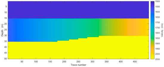
Figure 2.
Synthetic Earth model. In the layer below the sea floor, the velocity increases from 1600 to 2000 m/s from left to right, and the layer thickness decreases from 20 to 15 m. We simulated 50 traces, equally spaced from left to right along the model.
Figure 3a allows comparing of the estimated layer velocity and thickness obtained when jointly inverting all mentioned primaries and multiples (black circles) by tomography, i.e., by minimizing the object functions (11) or (22). The red circles are obtained instead by using the Equations (9) and (10), based on Dix Formula (7) as post-processing of the inversion in the angle domain. The blue dots correspond to the true model values. We see that the tomographic solutions in the velocity-thickness domain (black circles) are quite scattered, although close to the correct solution. The solution in the angles’ domain (green circles) is just perfect, nicely overlapping the true solution (blue dots). The Dix solution (red circles) are smoothly coherent but systematically lower than the true ones. We then added random errors in the travel times, perturbing each trace 10 times, to simulate picking errors or some noise contribution in the field records, as ambient noise or other interfering events. As a result, we get a mild scattering when the maximum noise percentage is 0.001% (Figure 3b) and significant for 0.01% (Figure 3c). In all cases, the Dix solutions rarely exceed the boundary traced by the blue dots, ending up as a slightly lower dispersion.

Figure 3.
Inversion estimates for 50 traces using tomography for layer parameters (black circles), angles (green circles) and with a Dix post-processing (red circles). The true model values are indicated by blue dots. The results’ scattering depends a lot on the maximum error percentage in the travel times: none (a), 0.001% (b) and 0.01% (c).
The travel times we are inverting range from a minimum value 2.937 ms of direct arrivals to a maximum of 89.210 ms for a “simple” multiple. For an intermediate value of 50 ms, the corresponding maximum percentage error is 5 microseconds for a 0.01% maximum percentage. This value corresponds to a tiny sampling interval, at a limit for standard instruments. Using percentage perturbations instead of fixed values reflects the different precision we expect when picking the seismic traces. The direct arrival Tdir and the reflection from the sea floor Tsf have better precision with respect to those of the deeper primary and the multiples. The first two events have a clear waveform with a sharp amplitude burst with respect to the ambient noise, while the latter signals are much weaker and often interfere with others. Thus, the late arrivals from multiples are prone to larger errors than the early ones.
Figure 4 shows the improvement we get by averaging the solution obtained by perturbing the same trace. While Figure 4a is just the (unperturbed) copy of Figure 3a, the trend of the averaged solutions is cleaner and quite similar to the unperturbed solution for a 0.001% (Figure 4b), while the dispersion increases for the 0.01% case (Figure 4c).
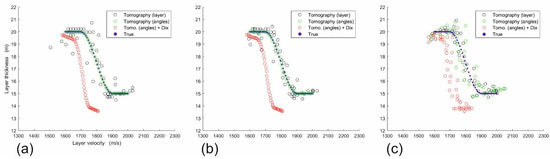
Figure 4.
Average values at each trace for the inversion using tomography for layer parameters (black circles), angles (green circles) and with a Dix post-processing (red circles). The maximum error percentage in the travel times is the same as in Figure 3: none (a), 0.001% (b) and 0.01% (c).
Further improvements can be obtained by a third-order median filter (Figure 5), when applied to the averaged data in Figure 4. In all three cases, the solution points are gathered along a more continuous trend. This flatter continuity is forced here mathematically, but it may be acceptable from a geological point of view: often lateral facies variations are smooth in nature. If we have the “a priori” information that this happens in the investigated area, it makes sense using it to enhance our estimates.

Figure 5.
Median filtering of order 3 of the values in Figure 4, i.e., using tomography for layer parameters (black circles), angles (green circles) and with a Dix post-processing (red circles). The maximum error percentage in the travel times is the same as in Figure 3: none (a), 0.001% (b) and 0.01% (c).
Figure 6 illustrates what happens when the maximum travel time errors become significant, i.e., 0.03%: an average value of 50 ms corresponds to 15 microseconds, which is more realistic for experimental data. We perturbed the travel times at each trace 10 times, getting the chaotic distribution in Figure 6a. However, taking the average of the values at each trace (Figure 6b) and then a 3-term median filter along the profile (Figure 6c), we get solutions that are not brilliant, but not too far from the correct solution (blue dots) either.
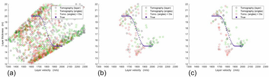
Figure 6.
Perturbations of 10 traces using tomography for layer parameters (black circles), angles (green circles) and with a Dix post-processing (red circles). The maximum error percentage in the travel times is 0.03%: all values (a), averaged values at each trace (b) and median filtering of the averaged points (c).
3.2. Real Data Example
Keeping in mind the limits highlighted by the synthetic example, we further tested our algorithms with a real data set. We processed a high-resolution monochannel seismic profile acquired at the Cavazzo Lake (Eastern Alps, Italy) with an UWAK 05 (Nautiknord) electro-dynamic sound source connected to a Pulsar 2002, with an output power 150–300 Joule/shot. The transducer generates broad-band (400–4000 kHz) seismic pulses. The reflected signals were acquired by a single-trace EG&G streamer, towing an 8 hydrophones array, 2.8 m long. Seismic data were processed by FOCUS Paradigm software package. The processing sequence included just two steps: amplitude recovery, compensating for the spherical divergence and anelastic absorption, and time-variant bandpass filtering. For the P velocity of the water, we used a value of 1446 m/s, as reported by [37]. Such a value is low with respect to typical values close to 1500 m/s normally encountered at sea, but nicely fits the values predicted by the McKenzie [31] empirical formula for cases with low temperature and low salinity, as encountered in alpine lakes.
Figure 7 shows a seismic section after the basic processing mentioned above. We see a strong direct arrival at less than 2 ms and a clear reflection for the lake floor between 10 ms (on the left) and 13 ms (on the right). Harder rocks outcrop on the left, while a small basin with a very different seismic stratigraphy is visible at the center and at right. We selected 100 traces indicated by the green rectangle, between shot 1697 and 1931, because the interpretation and picking of the key events is reliable, especially when taking into account the full picture.
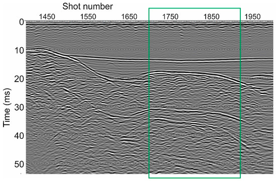
Figure 7.
Seismic section acquired at the Cavazzo Lake (Eastern Alps, Italy), using a Boomer system. The green rectangle displays the region where primaries and multiples were picked and inverted, from shot point 1697 to 1931.
Figure 8 displays a zoomed detail with the picked horizons: the lake floor (violet line), the base of the shallow sediments (yellow line), peg-leg multiple (red line) and simple multiple (green line). We could find a reliable, continuous signal for the possible intra-bed multiple in the shallow layer, so we did include that signal in the inversion engine.
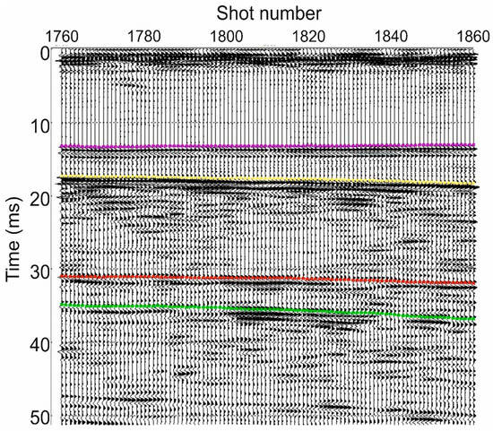
Figure 8.
Expanded detail with picked horizons of the central part of Figure 7, from shot point 1760 to 1860: lake floor (violet), base of shallow sediments (yellow), peg-leg multiple (red) and simple multiple (green).
We carried out the tomographic inversion in the angle domain, constraining the layer velocity to range from 1446 m/s (measured water velocity in the lake) to 2500 m/s. Figure 9 displays the estimated velocity (blue line) after a 7-term median filtering to remove a few sparse spikes in the inversion result. The velocity range, between 1500 and 2200 m/s, is quite typical for unconsolidated sediments. The curve is quite smooth, except for two instabilities around shot numbers 1830 and 1900. The curve obtained by the post-processing of the tomographic inversion by the Dix formula (orange line) is even smoother and, as expected from the experience with the synthetic data, its values are lower than the tomographic estimate. However, they are not realistic from a physical point of view, so that their use is just in confirming the general trend provided by tomography.
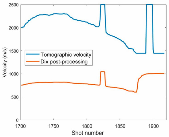
Figure 9.
Estimated velocities with a 7-term median filtering for the shallow layer, within the area highlighted in Figure 7: tomographic inversion in the angle domain (blue line) and with the Dix post-processing (orange line).
A relatively stable result is obtained for the thicknesses (Figure 10). The water depth (blue line) is just gently dipping, deepening slightly at the sides of the investigated area. The thickness of the shallow layer (red line) has some minor bumps at the same shot points as for the layer velocity (Figure 9), but its curve is almost overlapping its 7-term median filtered version (orange line), because the original estimate includes a few spikes only. We remark that such a continuity is driven by the data, as any trace is processed independently from any other.
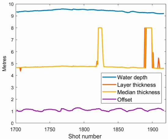
Figure 10.
Estimated water depth (blue line), layer thickness (red line), layer thickness after a 7-term median filtering (yellow line) and estimated offset from the direct arrivals (violet line).
In Figure 10 the lowest curve (violet line) shows the estimated offset, obtained by picking the direct arrival and dividing it by the water velocity. This curve is slightly bumpy, but with a kind of regularity, probably due to a feathering and variable tension of the trailed cable during the acquisition. Such a curve is not correlated at all with the thickness and velocity estimations, and this fact supports its reliability. The offset variations range from 0.98 to 1.24 m, which are quite large percentwise and so cannot be neglected (see also [27]).
4. Discussion
The median filter used to get Figure 5 from Figure 4 is just a third-order size, i.e., the shortest possible one. Longer filters can be chosen, of course, to highlight the low spatial frequency components of the velocity and thickness variations. This option should be used with care, however: if not supported by geological evidence, it introduces a personal bias from the interpreter.
Averaging traces acquired at the same location is a standard practice for land surveys, but is hardly feasible offshore. However, due to the small shot interval and the gentle lateral variations mostly encountered in the field, summing two or three adjacent traces into one may improve the signal/noise ratio in a similar way. Introducing proper weights in this summation, it is possible to also allow for some minor dips in the sea floor [38]. Other ways for improving the signal/noise ratio and so enhance the picking quality, include an FX deconvolution [39,40,41] and a data-driven compensation for geometrical spreading and anelastic absorption [25].
In our synthetic examples (Figure 3, Figure 4, Figure 5 and Figure 6), the Dix-formula post-processing provides more stable results (red circles) than the tomography in the layer-parameters domain (black circles), but underestimates both layer thickness and velocity for a percentage ranging from 1 to 10%. The reason is the mismatch between the simplified modelling used to simulate the travel times in the model (Figure 2) and the assumption of the Dix formula (Equation (7)). The latter one holds for Root Mean Square (RMS) velocities, defined for N layers [32]:
where T(0) is the travel time for a reflected event at offset zero, while Vi and Δti are the velocity and one-way propagation time in the i-th layer. The average velocity VA is instead:
Our travel time computation assumes straight ray paths, and thus the average velocity is actually implemented, instead of the RMS velocity assumed by the Dix formula. In our particular model their difference ranges from zero on the left side to 1% on the right side. When it comes to real data, the ray bending is better modelled by the RMS velocity, so the latter option may be more accurate when dealing with these synthetic data.
We remark that the zero-offset travel time T(0) is not measured directly in our case, as we have just a single non-zero offset trace available, but it is estimated from the multiple inversion using the ratio LV in Equation (1). Therefore, these results cannot be compared directly with a pure Dix approach, which requires only primaries (and possibly direct arrivals) but at least two offsets.
The results obtained by processing a real data set are encouraging, when using the Dix formula as a stabilizing tool. The additional smoothing by median filtering, which may help if the noise level is high, was not really needed in this case.
5. Conclusions
We presented a tomographic approach for inverting the travel times of direct, primary and various multiple reflections in a monochannel seismic survey. This method extends a recent work by [27]. The addition of more multiples does not significantly improve what can be obtained by only one, unless we average a significant number of estimated values. Improvements may be obtained by a median filtering of the traces along the profile, so exploiting, as “a priori” information, the natural smoothness often encountered in shallow sediments.
Minor differences are noticed when inverting the travel times of primaries and multiples using two different kernels, i.e., in the time domain versus the angle domain. The different choice of the Earth model parameters is not the only reason for this. In the time domain, the four unknowns (thickness and velocity for both sea water and shallow sediments) are solved jointly in a strict sense, while in the angle domain a layer-stripping approach is applied: the sea-water parameters are solved first, and then used for getting those of the sediments. However, we cannot claim that one approach is far better than the other.
The application to real data is quite challenging, requiring very accurate travel time picking and a compensation for possible offset changes at each shot. As a result of occasional instabilities, we cannot claim that the estimated velocities and thicknesses are always precise; however, the general trend provided by tomography, in terms of lateral variations, seems reliable and usable for a semi-quantitative interpretation.
Author Contributions
L.B. contributed with the key ideas, the data acquisition and its processing; A.V. developed the mathematical algorithm, its software implementation and the basic text. Both authors contributed to the discussion, the conclusions and the final text revision. All authors have read and agreed to the published version of the manuscript.
Funding
This research received no external funding.
Data Availability Statement
The experimental data presented in this paper was acquired under confidentiality conditions. The synthetic example data and the developed MatLab code can be provided by the Corresponding Author (avesnaver@ogs.it) upon request.
Acknowledgments
We thank our colleagues at OGS that contributed to the Boomer data acquisition.
Conflicts of Interest
The authors declare no conflict of interest.
References
- Hite, D.; Fontana, P.M. Wide azimuth streamer acquisition: From field development to exploration applications, and back again. In Expanded Abstracts, Proceedings of the 10th International Congress SBGF, Rio de Janeiro, Brazil, 19–22 November 2007; SEG: Itupeva, Brasil, 2007; pp. 869–873. [Google Scholar] [CrossRef]
- Biondi, B.L. 3D Seismic Imaging; SEG: Tulsa, OK, USA, 2006; p. 247. [Google Scholar] [CrossRef]
- Pecholcs, P.I.; Lafon, S.K.; Al-Ghamdi, T.; Al-Shammery, H.; Kelamis, P.; Huo, S.X.; Winter, O.; Kerboul, J.B.; Klein, T. Over 40,000 vibration points per day with real-time quality control: Opportunities and challenges. In Expanded Abstracts, Proceedings of the SEG Annual Meeting, Denver, CO, USA, 17–22 October 2010; SEG: Denver, CO, USA, 2010; pp. 111–115. [Google Scholar] [CrossRef]
- Pecholcs, P.I.; Al-Saad, R.; Al-Sannaa, M.; Quingley, J.; Bagaini, C.; Zarkidze, A.; May, R.; Guellili, S.; Membrouk, M. A broadband full azimuth seismic study from Saudi Arabia using a 100,000 channel recording system at 6 terabytes per day: Acquisition and processing lessons learned. In Expanded Abstracts, Proceedings of the SEG Annual Meeting, Las Vegas, NV, USA, 4–9 November 2012; SEG: Las Vegas, NV, USA, 2012; pp. 1–5. [Google Scholar] [CrossRef] [Green Version]
- Landais, M.; Mensch, T.; Grenie’, D.; Wombell, R. Broadband wide-azimuth towed streamer acquisition in West Africa. In Expanded Abstracts, Proceedings of the 84th SEG Annual Meeting, Denver, CO, USA, 26–31 October 2014; SEG: Denver, CO, USA, 2014; pp. 138–142. [Google Scholar] [CrossRef]
- Lin, L.F.; Hsu, H.H.; Liu, C.S.; Chao, K.H.; Ko, C.C.; Chiu, S.D.; Hsieh, H.S.; Ma., Y.F.; Chen, S.C. Marine 3D seismic volumes from 2D seismic survey with large streamer feathering. Mar. Geophys. Res. 2019, 40, 619–633. [Google Scholar] [CrossRef] [Green Version]
- Moldoveanu, N.; Nesladek, N.; Vigh, D. Wide-azimuth towed-streamer and large-scale OBN acquisition: A combined solution. In Expanded Abstracts, Proceedings of the 90th SEG Annual Meeting, Online, 11–16 October 2020; SEG: Houston, TX, USA, 2020; pp. 16–21. [Google Scholar] [CrossRef]
- Krief, M.; Garat, J.; Stellingwerff, J.; Ventre, J. A petrophysical interpretation using the velocities of P and S waves. Log Anal. 1990, 31, 355–369. [Google Scholar]
- Castagna, J.P.; Backus, M.M. (Eds.) Offset-Dependent Reflectivity—Theory and Practice of AVO Analysis; SEG: Tulsa, OK, USA, 1993; p. 357. [Google Scholar] [CrossRef]
- Russell, B.H.; Hedlin, K.; Hilterman, F.J.; Lines, L.R. Fluid-property discrimination with AVO: A Biot-Gassmann perspective. Geophysics 2003, 68, 29–39. [Google Scholar] [CrossRef] [Green Version]
- Ikelle, L.; Amundsen, L. Introduction to Petroleum Seismology; SEG: Tulsa, OK, USA, 2005; p. 706. ISBN 978-1560801290. [Google Scholar]
- Carcione, J.M. Wave Fields in Real Media, 3rd ed.; Elsevier: Amsterdam, The Netherlands, 2015; ISBN1 9780080999999. ISBN2 9780081000038. [Google Scholar]
- Mesdag, P.; Quevedo, L.; Tănase, C. Enabling isotropic reflectivity modeling and inversion in anisotropic media. Lead. Edge 2021, 40, 267–276. [Google Scholar] [CrossRef]
- Trabant, P.K. Applied High-Resolution Geophysical Methods; Springer: Dordrecht, The Netherlands, 1984; p. 265. ISBN 978-94-009-6495-2. [Google Scholar]
- Gordon, J.; Gillespie, D.; Potter, J.; Frantzis, A.; Simmonds, M.P.; Swift, R.; Thompson, D. A review of the effects of seismic surveys on marine mammals. Mar. Technol. Soc. J. 2003, 37, 16–34. [Google Scholar] [CrossRef] [Green Version]
- Bini, A.; Corbari, D.; Falletti, P.; Fassina, M.; Perotti, C.R.; Piccin, A. Morphology and geological setting of Iseo Lake (Lombardy) through multibeam bathymetry and high-resolution seismic profiles. Swiss J. Geosci. 2007, 100, 23–40. [Google Scholar] [CrossRef]
- Baradello, L.; Carcione, J.M. Optimal seismic-data acquisition in very shallow waters: Surveys in the Venice lagoon. Geophysics 2008, 73, Q59–Q63. [Google Scholar] [CrossRef]
- Tosi, L.; Rizzetto, F.; Zecchin, M.; Brancolini, G.; Baradello, L. Morphostratigraphic framework of the Venice Lagoon (Italy) by very shallow water VHRS surveys: Evidence of radical changes triggered by human-induced river diversions. Geophys. Res. Lett. 2009, 36, 1–5. [Google Scholar] [CrossRef]
- Romeo, R.; Baradello, L.; Blanos, R.; Congiatu, P.P.; Cotterle, D.; Ciriaco, S.; Donda, F.; Deponte, M.; Gazale, V.; Gordini, E.; et al. Shallow geophysics of the Asinara Island Marine Reserve Area (NW Sardinia, Italy). J. Maps 2019, 15, 759–772. [Google Scholar] [CrossRef] [Green Version]
- Verbeek, N.H.; McGee, T.M. Characteristics of high-resolution marine reflection profile sources. J. Appl. Geophys. 1995, 33, 251–269. [Google Scholar] [CrossRef]
- Mosher, D.C.; Simpkin, P.G. Status and trends of marine high-resolution seismic reflection profiling: Data acquisition. Geosci. Can. 1999, 26, 174–188. [Google Scholar]
- Müller, C.; Milkereit, B.; Bohlen, T.; Theilen, F. Towards high-resolution 3D marine seismic surveying using Boomer sources. Geophys. Prospect. 2002, 50, 517–526. [Google Scholar] [CrossRef]
- Müller, C.; Woelz, S.; Ersoy, Y.; Boyce, J.; Jokisch, T.; Wendt, G.; Rabbel, W. Ultra-high-resolution 2D-3D seismic investigation of gthe Liman Tepe/Karantina Island archeological site (Urla/Turkey). J. Appl. Geophys. 2009, 68, 124–134. [Google Scholar] [CrossRef] [Green Version]
- Vesnaver, A.; Busetti, M.; Baradello, L. Chirp data processing for fluid flow detection at the Gulf of Trieste (Northern Adriatic Sea). Bull. Geophys. Oceanogr. 2021, 62, 365–386. [Google Scholar] [CrossRef]
- Denich, E.; Vesnaver, A.; Baradello, L. Amplitude recovery and deconvolution of Chirp and Boomer data for marine geology and offshore engineering. Energies 2021, 14, 5704. [Google Scholar] [CrossRef]
- Vesnaver, A.; Baradello, L. Shallow velocity estimation by multiples in Boomer surveys. In Extended Abstracts, Proceedings of the EAGE Annual Meeting, Madrid, Spain, 22–24 May 2022; EAGE: Madrid, Spain, 2022; p. 195, in press. [Google Scholar]
- Vesnaver, A.; Baradello, L. Shallow velocity estimation by multiples for monochannel Boomer surveys. Appl. Sci. 2022, 12, 3046. [Google Scholar] [CrossRef]
- Nemeth, T.; Sun, H.; Schuster, G.T. Separation of signal and coherent noise by migration filtering. Geophysics 2000, 65, 574–583. [Google Scholar] [CrossRef]
- Xu, S.; Chen, F.; Tang, B.; Lambare’, G. Noise removal by migration of time-shift images. Geophysics 2014, 79, S105–S111. [Google Scholar] [CrossRef]
- Vesnaver, A.; Accaino, F.; Böhm, G.; Madrussani, G.; Pajchel, J.; Rossi, G.; Dal Moro, G. Time-lapse tomography. Geophysics 2003, 68, 815–823. [Google Scholar] [CrossRef]
- Mackenzie, K.V. Nine-term equation for sound speed in the oceans. J. Acoust. Soc. Am. 1981, 70, 807–812. [Google Scholar] [CrossRef]
- Hubral, P.; Krey, T. Interval Velocities from Seismic Reflection Time Measurements; SEG: Tulsa, OK, USA, 1980; p. 203. ISBN 0-931830-13-3. [Google Scholar] [CrossRef]
- Robein, E. Velocities, Time-imaging and depth-imaging in reflection seismics. In Principles and Methods; EAGE: Houten, The Netherlands, 2003; p. 464. ISBN 90-73781-28-0. [Google Scholar]
- Press, W.H.; Flannery, B.P.; Teukolski, S.A.; Vetterling, W.T. Numerical Recipes, 3rd ed.; Cambridge University Press: Cambridge, UK, 2007; p. 1256. ISBN 9780521880688. [Google Scholar]
- Van der Sluis, A.; Van der Vorst, H.A. Numerical solution of large, sparse linear algebraic systems arising from tomographic problems. In Seismic Tomography with Applications in Global Seismology and Exploration Geophysics; Nolet, G., Ed.; Reidel: Dordrecht, The Netherlands, 1987; pp. 49–83. [Google Scholar]
- Vesnaver, A. Towards the uniqueness of tomographic inversion solutions. J. Seism. Explor. 1994, 3, 323–334. [Google Scholar]
- Polonia, A.; Albertazzi, S.; Bellucci, L.G.; Bonetti, C.; Giorgetti, G.; Giuliani, S.; López Correa, M.; Mayr, C.; Peruzza, L.; Stanghellini, G.; et al. Decoding a complex record of anthropogenic and natural impacts in the Lake of Cavazzo sediments NE Italy. Sci. Total Environ. 2021, 787, 1–18. [Google Scholar] [CrossRef]
- Biswell, D.E.; Konty, L.F.; Liaw, A. A geophone subarray beam-steering process. Geophysics 1984, 49, 1838–1849. [Google Scholar] [CrossRef]
- Canales, L. Random noise reduction. In Expanded Abstracts, Proceedings of the 54th Annual International Meeting, Atlanta, Georgia, 2–6 December 1984; SEG: Atlanta, GA, USA, 1984; pp. 525–527. [Google Scholar] [CrossRef]
- Gulunay, N. FX decon and complex Wiener prediction filter. In Expanded Abstracts, Proceedings of the 56th Annual International Meeting, Houston, TX, 2–6 November 1986; SEG: Houston, TX, USA, 1986; pp. 279–281. [Google Scholar] [CrossRef]
- Baradello, L. An improved processing sequence for uncorrelated Chirp sonar data. Mar. Geophys. Res. 2014, 35, 337–344. [Google Scholar] [CrossRef]
Publisher’s Note: MDPI stays neutral with regard to jurisdictional claims in published maps and institutional affiliations. |
© 2022 by the authors. Licensee MDPI, Basel, Switzerland. This article is an open access article distributed under the terms and conditions of the Creative Commons Attribution (CC BY) license (https://creativecommons.org/licenses/by/4.0/).