Article

Assessment of Ground Instabilities’ Causative Factors Using Multivariate Statistical Analysis Methods: Case of the Coastal Region of Northwestern Rif, Morocco

by
Haytam Tribak
1,2,3,*,
Muriel Gasc-Barbier
1,* and
Abdelkader El Garouani
2
1
GeoCoD, Cerema, 13290 Aix en Provence, France
2
Functional Ecology and Environmental Engineering Laboratory, Sidi Mohamed Ben Abdellah University, Fez 30050, Morocco
3
Géoazur, Côte d’Azur University, 06560 Valbonne, France
*
Authors to whom correspondence should be addressed.
Geosciences 2022, 12(10), 383; https://doi.org/10.3390/geosciences12100383
Submission received: 1 September 2022 / Revised: 11 October 2022 / Accepted: 11 October 2022 / Published: 14 October 2022
(This article belongs to the Collection New Advances in Geotechnical Engineering)

Abstract

:
An assessment of ground instabilities’ causative factors remains a topical subject. Such studies are rare, and evaluation techniques are still under development. The choice of evaluation technique should take into account the materials available and the objective sought. Statistical analysis methods are the most widely used, with multivariate analysis being the most accurate. The present work evaluates the weights of the influences of the different factors of ground instability of the coastal region between Tetouan and Jebha through multiple correspondence analysis (MCA) and principal component analysis (PCA). The application of both methods requires an accurate ground instability inventory with study sites that are well documented through modalities of causative factors and other descriptive data. The performed MCA shows that lithology has a significant influence on the type of existing instability. It also helped classify the instabilities into five distinct classes according to their modalities and specify the factors that differentiate the classes. The PCA shows that lithology is the most influential factor in landslides, contrary to rockfalls, where a variety of factors can be preponderant.

1. Introduction

Ground instabilities are the most catastrophic geohazards in many areas of the world [1,2,3]. Several internal or external factors can play a part in the initiation and reactivation of ground movements. These factors can have geological, geomechanical, geometric, hydrological, climatic, edaphic, or anthropogenic origins [4,5]. They control the type and spatial distribution of ground movements in the presence of other aggravating factors [6]. The importance of each factor depends on its degree of influence, i.e., its ability to determine the typology and frequency of existing land movements. Indeed, for each ground instability in a study area, the study in [7] demonstrated that one of the factors is preponderant, whereas other authors have often pointed out a combination of many factors [8,9]. Weights assigned to causative factors differ, as the characteristics of conditioning factors vary from region to region [10,11]. Concerning the evaluation of the causative factors, most of the current works are focused on the analysis of the susceptibility of the ground movements through the association of various factors by means of statistical methods. The evaluation consists of the correlation of the susceptibility result with each tested factor. The best result attributes a weight to each factor in the analysis. There are very few methods of ranking the factors according to their influence weight; the best known method is to consider an expert’s judgment based on a visual interpretation of the interrelations between the parameters. However, expert approaches always present subjectivity and may lead to results that do not fully reflect reality. The important use of expert judgement is related to the quality and quantity of the data needed.
In this study, the evaluation of causative factors is not focused on the notion of risk or susceptibility. They are evaluated in connection to their interrelationships with respect to already existing instability phenomena. The interrelationship and correlation between causative factors can only be obtained by factor analysis techniques [12]. The choice of a proper technique depends on the input data. The coastal region between Tetouan and El Jebeha is an ideal place for this type of analysis due to the presence of the majority of the instability factors commonly found in the literature. Many instabilities can be found in the area, with different factor modalities. Therefore, the present work opts for an evaluation of the degree of influence of the causative factors, mainly the predisposition causative factors, using a multivariate statistical approach. This is performed with a descriptive discriminant analysis based on principal component analysis (PCA) and multiple correspondence analysis (MCA).

2. Studied Area

The area is located at the northwest of Morocco (Figure 1). It lies along the Mediterranean coast with an area of 763 km2. It is divided between two provinces, Tetouan and Chefchaouen. The region is subject to different types of climates (Mediterranean, oceanic, continental, mountain) and is crossed by many watercourses flowing into the Mediterranean Sea.
The area contains many geomorphological features, resulting mainly from structural, hydrological and climatic factors. It constitutes a zone for several dynamic and interactive processes at different spatial and temporal scales. Reliefs are rough and the slopes are very steep with valleys that are strongly incised [13]; these conditions account for the occurrence of various natural disasters (floods, mass movements, etc.). The study area is represented by four structural units: Sebtides, Ghomarides, Calcareous Dorsale, and Flysch domain. They are formed by thrust sheets resulting from a complex orogenic process deriving from a collision during the Lower Miocene between the northwestern African margin and the Alboran plate [14,15]. The Alboran plate detached from the southeastern margin of the Iberian–Sardinian plate in the Oligocene [16,17]. Sebtides, Ghomarides, and Calcareous Dorsale belong to the internal domain of Rif, composed by ultrabasic, metamorphic, and carbonate rocks. The Flysch domain is constituted by sandstone–pelite and marl–calcareous rocks (Figure 2).
To assess the frequency and dispersion of ground instabilities and to know whether an area deserves special attention and further study, a detailed inventory containing the typology and distribution of ground instabilities is of primary importance. Such an inventory was realized in the studied area [19] and will be the support of our ground instability assessment (Figure 3). A total of 342 ground instabilities have been recorded, including 163 landslides, 39 rockfalls, 77 gullies, and 63 road slope collapses. Figure 4 show an example of four ground instabilities, and their precise locations are shown in Figure 3.

3. Materials and Methods

3.1. Methodology

The causative factors of ground instabilities were assessed using two major multivariate statistical analysis methods: multiple correspondence analysis (MCA) and principal component analysis (PCA).
MCA is a descriptive technique that makes it possible to study the association between at least two qualitative variables [20]. MCA allows the acquisition of representations on which the proximities between the subsets of the modalities of qualitative variables can be observed. It can aim to synthetize the information contained in many variables in order to facilitate the interpretation of existing correlations between those variables. In the present work, MCA helped mainly to provide classes of instabilities, i.e., to analyze similarities between the different studied sites in a multidimensional perspective in order to determine the number and modalities of the classes. Correlations between the qualitative instability factors were then evaluated to determine which ones intervene the most in determining the ground instability classes. Finally, an additional variable “type of instability” was introduced to correlate with instability factors in order to observe the possible links between them and thus post-validate the analysis.
PCA is an extremely powerful tool for compressing and synthesizing information, which is very useful when there is a large amount of quantitative data to process and interpret [21]. It allows for correlations between quantitative variables to be visualized and interpreted, even if they are dichotomous, in order to limit the number of variables and only keep those that are important in the analysis. In our study, the objective in using PCA was to represent the quantitative instability factors and to visualize their correlations in order to classify the factors according to their degree of importance. It also had a comparative purpose: the PCA results were compared to the MCA results in order to improve interpretations.
The evaluation of the causative factors was based on both the MCA and PCA results. The “FactoMineR” package of the programming language R [22] was used for the numerical application of the two methods.

3.2. Materials

3.2.1. Exploitation of the Inventory

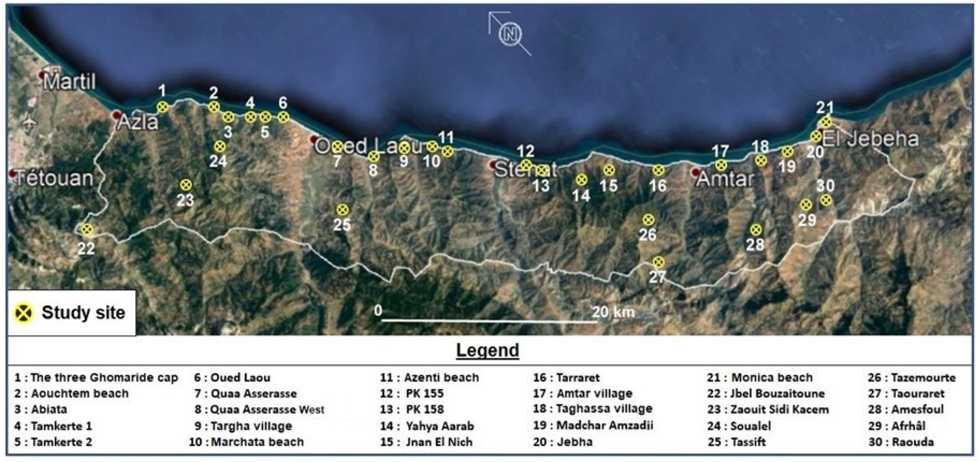
The obtained ground instability inventory constituted the first element that was analyzed. Among the 342 instabilities inventoried, 30 typical sites were designated to constitute the data sources that fed the statistical analyses. The choice of sites was determined based on a combination of several criteria. Geographically, the sites were chosen to cover the whole area, although the distribution map (Figure 5) shows that most of the sites are located along the coastline. The reason for this is that most ground instabilities are also located along the coastline. The study sites were selected to be at different altitudes to test the different types of climates of the region and confront more parameters responsible for instabilities. We chose to select all lithologies encountered as well as all the structural units of the area. The aim was to confront all the geological data with ground instabilities to understand their influence on the latter.
The same principle was applied to the other tested parameters: geometric, hydrological, anthropic aspects, etc. The sites were chosen to be representative of the different ground instability types existing in the study area. All types of landslides, except for mudflows, were considered. As many rockfalls occur in the area, we only considered those with a minimum volume of 10 m3.

3.2.2. Study Site and Input Data

Each selected site was analyzed in-depth to identify the potential predisposing factors that could have participated in the triggering of ground movement. Data were collected from different sources, including field trips, thematic maps, state databases, modeling and data reprocessing in GIS software, etc. Table 1 presents the variables used in MCA and Table 2 presents the variables used in PCA. Appendix A provides the datasets used in our statistical analyses: Table A1 presents the MCA input data, Table A2 presents the PCA input data for the landslide portion, and Table A3 presents the PCA input data for the rockfall portion.
The processed data are both qualitative and quantitative. Some MCA variables are found in the PCA as quantitative variables, whereas others are specific to PCA. In PCA, we decided to independently process landslide and rockfall as the mechanics of the movements is different. Thus, the same variable may not have the same influence weight in both cases. In both PCAs, elevation was considered as an additional variable because it disturbs the other variables.
In the landslide PCA dataset, we decided to add some geomechanical parameters: cohesion, C and friction angle, Φ. Considering where landslide occurred, cohesion and friction angle are calculated on each site by a retro-analysis at limit equilibrium. Thus, the set of parameters (C and Φ) that gives a factor of safety equal to one is calculated for each given geometrical description. Numerical modeling of each landslide was performed with FLAC/slope [23]. As it was not possible to carry out precise soil studies on each site, we had to access part of our geotechnical parameters from existing literature. Thus, C and Φ are linked together. Thus, they are additional variables in the analysis. The interest of their presence is to examine their correlations with the other active variables.
In the PCA rockfall, cohesion is considered to be equal to zero as the rocks failed; thus, no cohesion value is included in the analysis. In the meantime, we decided to include the number of geometrical instabilities in the analysis. Indeed, from a stability analysis point of view, it is the geometrical repartition of discontinuities that create potentially instable rock blocks. As it was not possible to compute all sites with statistically acceptable discontinuity sets [24], we decided to simplify the approach and to consider the number of geometrical instabilities obtained on each site with a simple analysis of the stereograms [25].

4. Results and Discussion

4.1. Multiple Correspondence Analysis (MCA)

4.1.1. Choice of Factorial Design and Distribution of Inertia

The inertia of an axis measures the link between the axis and the variables. The percentage of inertia given by each axis expresses the quantity of information provided by the axis. In MCA, the percentage of inertia is low depending on the number of individuals, qualitative variables and their modalities. Determining the MCA number of factorial axes is tricky. The most commonly used criteria in factor analysis to select the axes to be interpreted are Keiser’s criterion [26] and Coude’s criterion [27]. Here, neither of them can be used. Keiser’s criterion suggests that the first 10 axes should be interpreted and, as we will observe later, only the first four axes can be used. Coude’s criterion requires a significant decay between one axis and another, which is not the case in our inertia diagram. In the present work, the choice of the factorial plans will use a criterion that focuses on the axes regrouping the greatest number of modalities of the variables that contribute to their construction. Axes 1 and 2 correspond to the dimensions that have the highest percentage of inertia (25.9%) and that group most of the studied modalities (Figure 6).

4.1.2. Data Contribution to the Axes

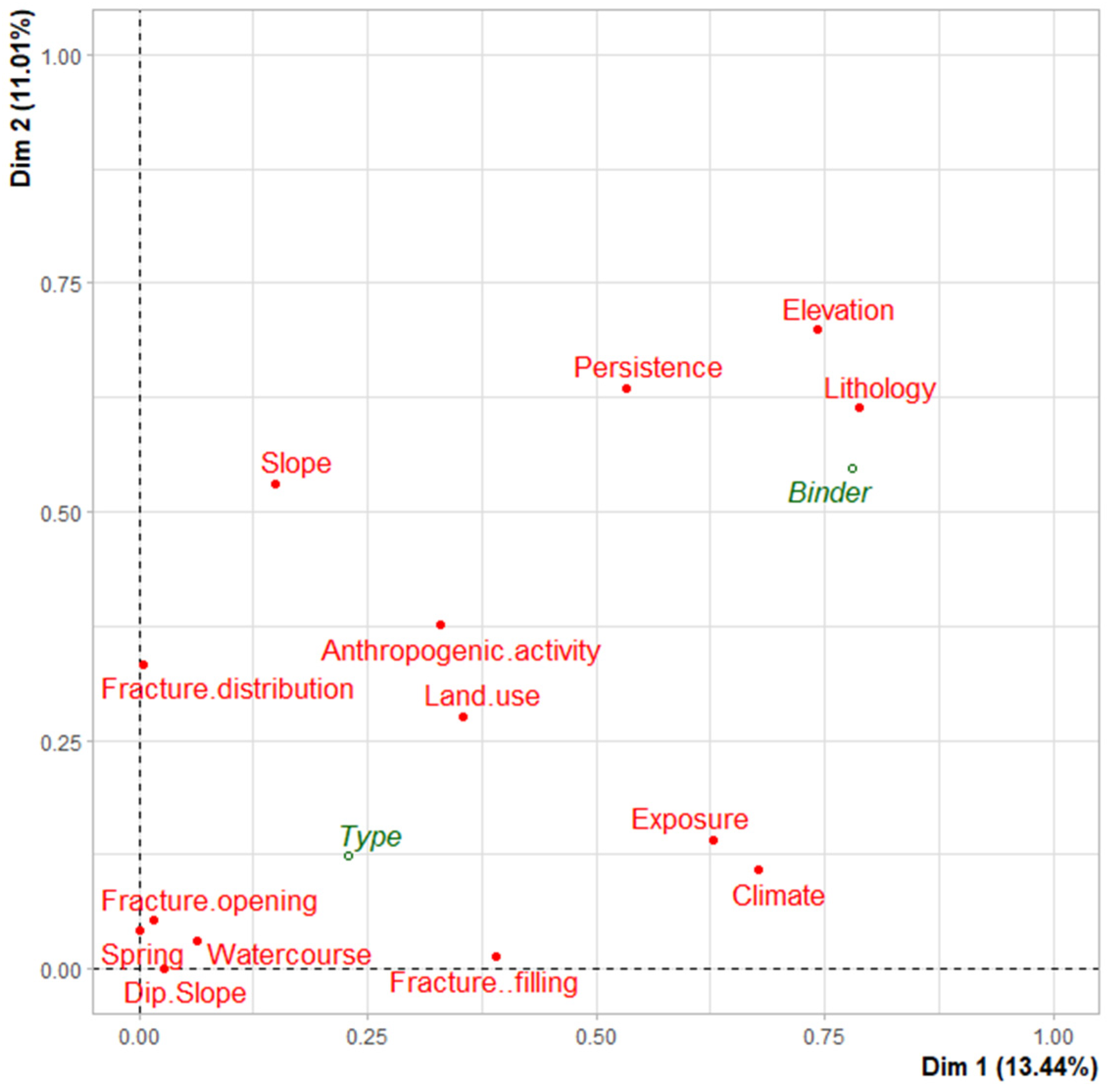
There are 63 modalities in the analysis, 55 of which are active and 11 are additional. For a critical probability of 0.05, axis 1 is represented by 10 variables and 24 modalities. The variable “Lithology” is the most related to axis 1 with a correlation ratio of 0.789. Axis 2 is represented by eight variables with the variable “Elevation” being the most related to it. Except for “Watercourse”, “Spring”, “Dip/slope”, and “Fracture opening”, all other variables are well represented along axes 1 and 2 (Figure 7). Similarly for the individuals, the more a study site contains rare modalities, the further it is from the center of the graph and the more it contributes to the formation of the axes.

4.1.3. Interpretation of Graphs

  • Geological variables
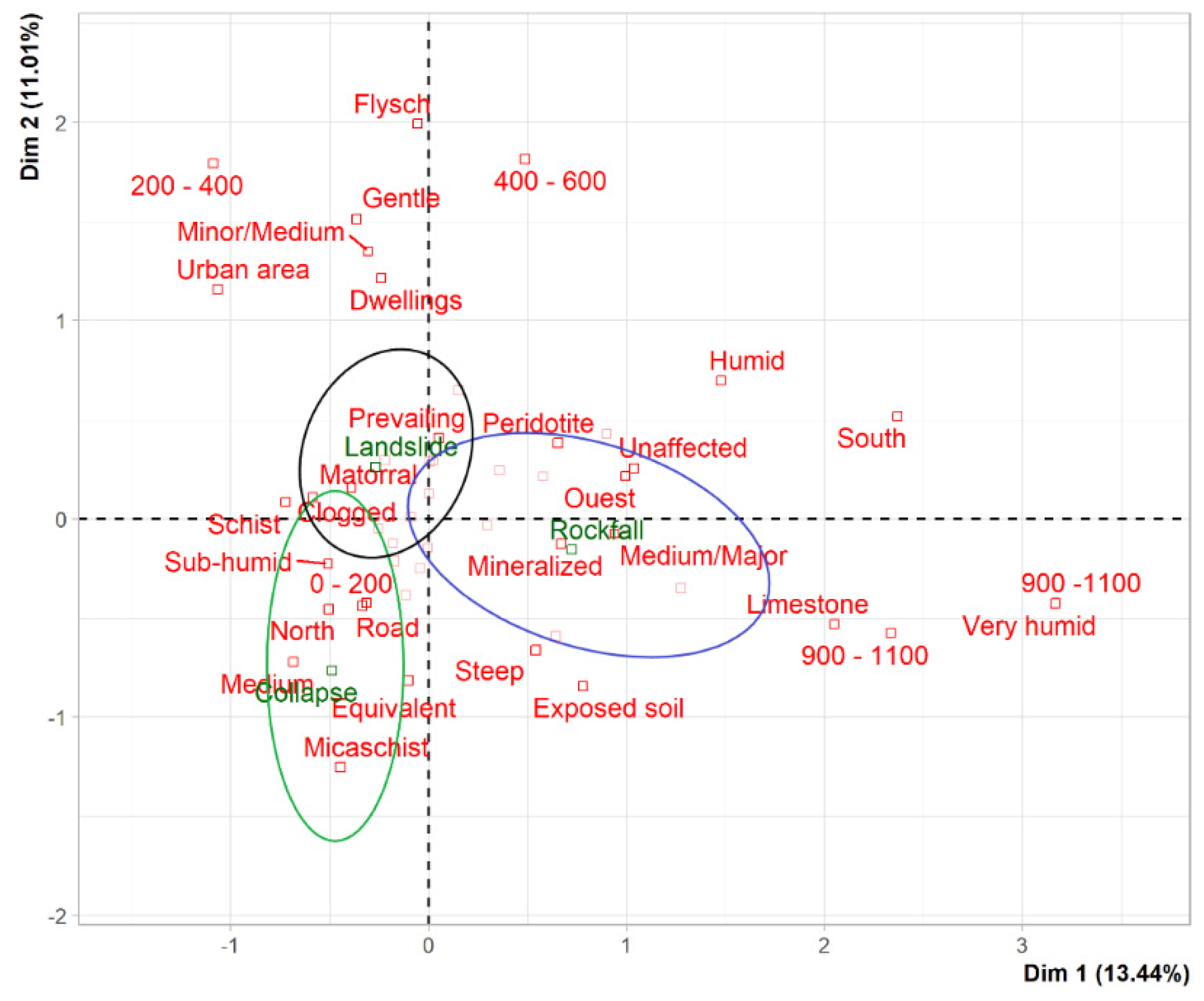
Observing the modalities graph (Figure 8), we notice a large dispersion between lithologic modalities which explains the significant separation of the subsets of the study sites. Axis 1 discriminates between the less coherent rocks on the left and the more coherent rocks on the right. For the variable “Fracture persistence”, axis 1 shows an opposition between sites with a fracture size “Medium and Maj” on the right and “Medium” and “Min and Medium” on the left. Similarly, for the “Fracture Filling” variable, axis 1 contrasts the clogged fractures on the left and the mineralized fractures on the right. The distribution of the fractures is linked to axis 2. This opposes the prevailing systems at the top and the equivalent systems at the bottom.
  • Geometric variables
For the variable “Slope”, we notice a discrimination, according to axis 2, between sites with low slopes, at the top, and sites with high slopes, at the bottom. Most of the study sites have north- and east-facing slopes. Axis 1 contrasts north- and east-facing slopes on the left and those with west and south exposures on the right. The four modalities of the “Elevation” have a well-determined dispersion: axis 1 is opposing the sites with low altitudes on the left and the sites with high altitudes on the right. The variable “Dip/Slope” shows a heterogeneous and random dispersion of the modalities along the two axes.
  • Hydrological variables
The interpretation of the variable “Climate” is a bit particular as both axes are needed. According to the graph, axis 1 discriminates between sub-humid sites on the left and humid and very humid sites on the right. Therefore, we deduce, from the contribution of each modalities, that axis 1 is the humidity axis. On the other hand, axis 2 opposes the arid sites at the bottom and the semi-arid sites at the top. We can deduce that axis 2 is the axis that represents aridity. The modalities of the variables “Spring” and “Watercourses” show no discrimination along either axis 1 or 2 or along the other dimensions.
  • Anthropogenic and land use variables
For the “Anthropogenic activity” variable, axis 1 discriminates sites affected by anthropogenic activity (roads, dwellings) on the left and those unaffected on the right. Axis 2 discriminates sites affected by dwellings at the top of the graph and sites affected by roads at the bottom. For the “Land use” variable, the confidence ellipses of the sub-individuals are well separated. We also notice discriminations along the two axes between the different modalities. Nevertheless, no logical interpretation could be drawn from the graph, except for the fact that the sites where the soils are occupied by anthropic activities are on the left of the axis and those unoccupied by anthropic activities are on the right of the graph.

4.1.4. Analysis and Interpretation of Correlations

One of the advantages of MCA is that it allows automatic correlations to be made between variables and modalities that are likely to behave in the same way. In the present work, an analysis of the correlations will allow us to understand the relationships between the correlated variables, which will allow us to evaluate the influence of the causative factors of ground instabilities. By analyzing the graphs of the variables and modalities (Figure 7 and Figure 8), we notice very strong correlations between certain variables and modalities whereas others are either less correlated or not correlated. We notice a connection between the variables “Lithology”, “Fracture persistence”, and “Elevation”. Hence, we can deduce that, in general, the more coherent a rock is, the bigger the fracture persistence, the higher the altitude, and vice versa. The link between the climate and the exposure of the slopes is expressed by the approximation of the modalities of aridity with the northern and eastern exposures and the modalities of humidity with the southern and western exposures. We also note a strong correlation between land use and anthropic activities. Forests and exposed soils are generally not occupied by anthropic activity, unlike matorrals and housing areas where we find high anthropic activity. Another correlation that appears in the graph is the relationship between the variable “Slope” and “Anthropogenic activity”. The closer we get to the “Road” modality, the steeper the slope and the more ground instabilities are encountered. On the other hand, the dwellings are more concentrated on gentle and light slopes where we notice very few ground instabilities. Some correlations appear to be completely illogical but deserve to be mentioned in order not to miss even minor information. Here, we talk about the correlation between the slope degree and the fracture distribution; indeed, we notice that the weak slopes of the dataset tend towards the prevailing system and the strong slopes towards the equivalent system.

4.1.5. Focus on the Additional Variable “Type”

In MCA, it is common for a variable to play a specific role in the sense that it is the one that we are trying to explain it from the others [28]; this is exactly the case of the additional variable “Type” in the dataset. This specific role eventually appears only at the level of interpretation. When this is the case, it means that MCA has worked well. In other words, the variables explaining the phenomenon (here the “Type” variable) have been taken into account and have been highlighted by the analysis. Here, we need to know the factors that control the type of ground instability. In the modalities graph, the type of instability is located at the barycenter of the modalities it contains. The confidence ellipses surrounding the barycenters contain the modalities that are related to the instability types. In the case of rockfalls, we find that they are concentrated in limestone terrain, high altitudes, steep slopes, humid climate, exposed soils, etc. Landslides are rather concentrated in schistose, sandstone, and peridotitic terrains, in matorrals, light slopes, medium altitudes, minor and medium fractures, etc. In addition to the connection between the modalities, the distances between them is added. The modality closest to an instability type is the most related to it. Although the quality of the representation of the instability types is very average, it can be seen from the figure that the lithological and structural factors are the closest and therefore the most influential.

4.2. Principal Component Analysis (PCA)—Landslide Analysis

4.2.1. Choice of Factorial Design and Distribution of Inertia

In PCA, the inertia of the factorial axes indicates, on one hand, whether the variables are structured or not and on the other hand, suggests the appropriate number of principal components to study [29]. As in MCA, the choice of the factorial design was based on the variables’ contributions to the axes. For all variables to be taken into account in the analysis, the contributions must exceed a certain threshold. According to Kaiser’s criterion, the average inertia of the axes is equal to 10%. Consequently, the description of the analysis will be restricted to the axes that have a percentage greater than this value, corresponding to the first four axes, which represent 76.26% of the total inertia (Figure 9).

4.2.2. Data Contribution to the Axes

  • Interpretation of the individuals’ graph
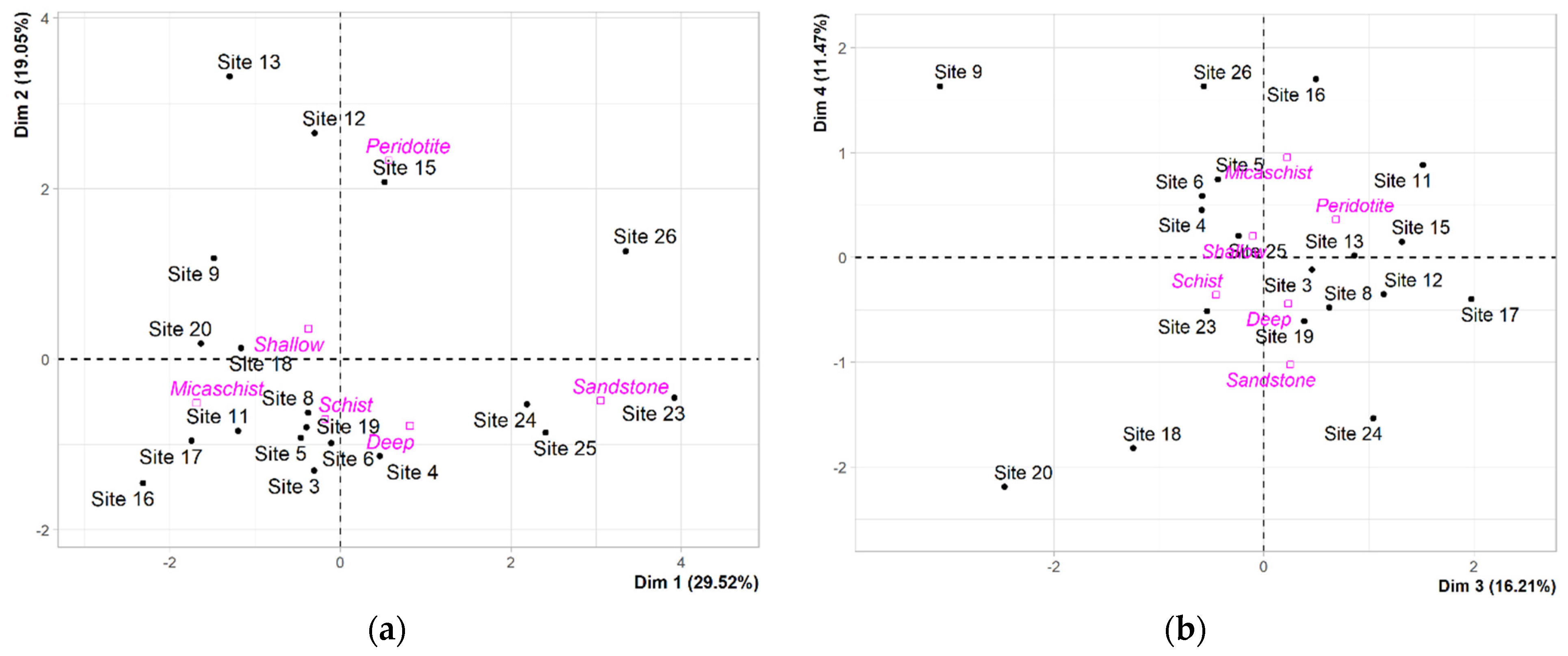
The individuals who contributed the most to the formation of the axes are those who have coordinates significantly different from zero and a contribution greater than the total average contribution. The latter has a value of 5.26%. In our case, sites 16, 23, and 26 strongly contributed to the formation of the first dimension; sites 12, 13, 15, 23, 24, and 25 contributed strongly to the second dimension; sites 8, 11, 17, 18, 20, 24, and 26 strongly contributed to the third dimension; and sites 9, 16, and 18 strongly contributed to the fourth dimension (Figure 10). According to the critical probability of Wilks’ test, the software suggests that the “Lithology” variable is the best qualitative variable for illustrating the distances between individuals on the factorial designs.
  • Interpretation of the graphs of variables
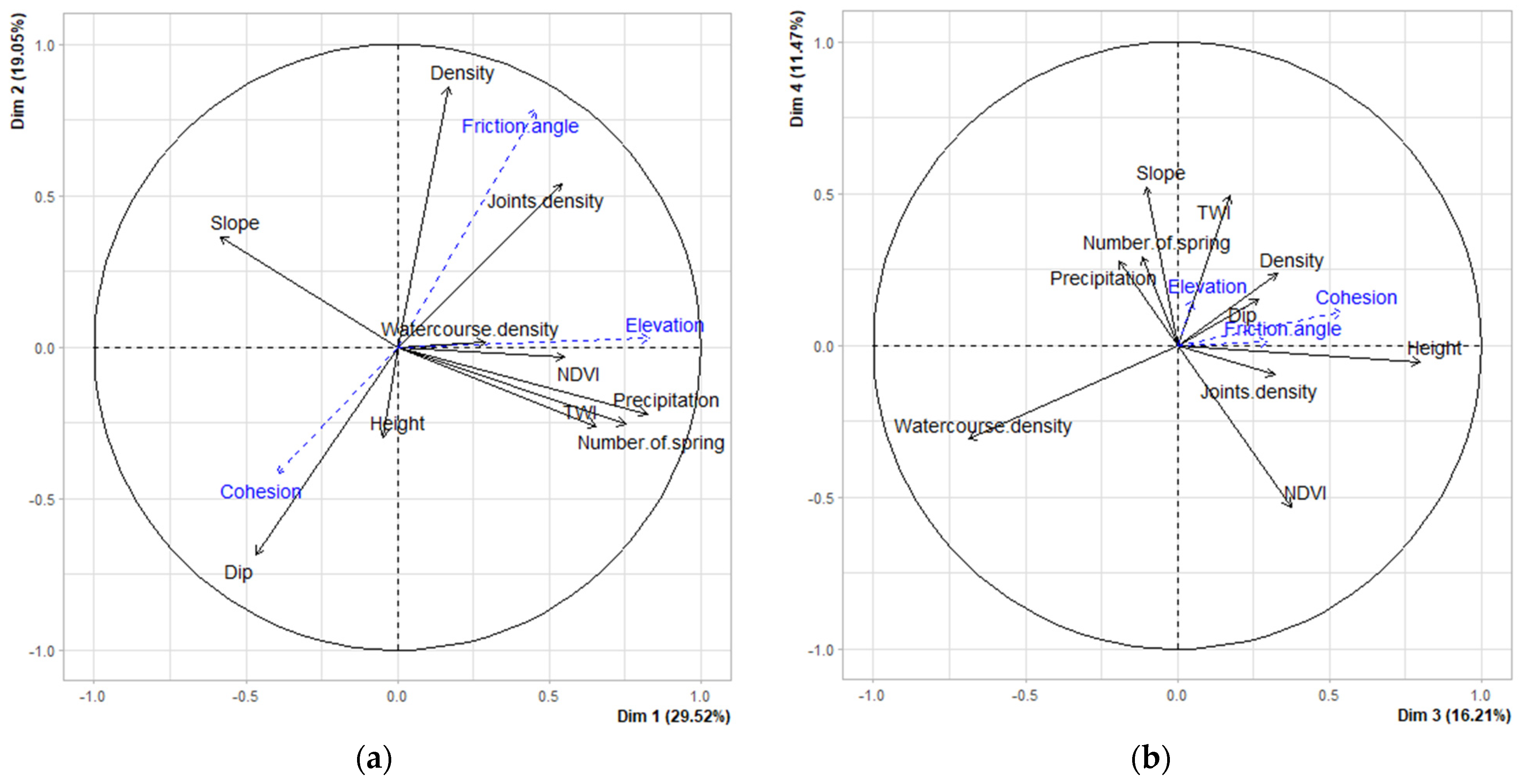
The interpretation of the correlations circle also considers their average contribution on the first four axes. Only the variables whose contribution is greater than 10% along each axis were interpreted. According to the correlation circles in Figure 11, we notice strong correlations between some variables (Density, Friction angle, and Joints discontinuity) which are positive on axis 1 and 2, whereas others (Elevation, Number of springs, Precipitation, and TWI) are positive on axis 1 and negative on axis 2. The variable “Dip” is negative on both axes. The “Height” and “Cohesion” variables are highly correlated on axis 3. The variables “Slope” with negative coordinates and “NDVI” with positive coordinates, are correlated to axis 4.

4.2.3. Study of Proximities between Points

The graph of the variables (Figure 11) gives an approximation of the correlations between the variables along the different axes: some variables are positively or negatively correlated, while the orthogonal variables are uncorrelated. The analysis of the correlations between the variables gives information about the possible links between two or more variables to determine if there is any influence of one on the other. It also indicates which are the solitary variables that do not depend on other variables.
According to the studied axes in Figure 11, the variables “Density”, “Friction angle”, and “Joints density” show a strong relationship as their values vary proportionally with each other. The same is true for the group of variables that consists of “Elevation”, “Precipitation”, “Number of springs”, and “TWI” and the group of variables that consists of “Cohesion” and “Height”. Others are negatively correlated, and their values are inversely proportional (“Slope” and “NDVI”, “Slope” and “TWI”). In the individual graphs (Figure 10), the distribution of sites is controlled by the values of the variables. We notice that the sites form groups (subclusters) controlled by specific variables. The analysis of the contributions of the individuals according to the different axes shows that there are two types of groups of individuals: the first is homogeneous and is controlled by very specific variables. The second is heterogeneous and is controlled by several variables at the same time. For example, the group (sites 12, 13, and 15) is strongly related to the second dimension controlled by the lithological variables (Friction angle and Density). The group (sites 23 and 26) is strongly linked to the first dimension controlled by the variables (Joint density, Precipitation, Number of springs, and Elevation). We also notice some solitary individuals linked to specific variables, e.g., sites 9 and site 20 are linked to the fourth and fifth dimensions, where the variables “Watercourses density”, “NDVI”, “Slope”, and “TWI” dominate. Other individuals (e.g., sites 3, 4, 5, and 8) are not linked to any dimension and thus do not depend on specific variables. These individuals generally share almost the same values of the variables and those values are close to the general average of the values. In this case, the variables share the same force applied on the individuals. In general, the proximities between individuals are clearly represented along axis 1 and 2, controlled by the geological and hydrological variables and schematized by the illustrative variable “Lithology”.

4.2.4. Analysis and Interpretation of Correlations

According to the correlation circles (Figure 11a,b), the variables “Elevation”, “Precipitation”, and “Number of springs” show a strong correlation. This can be explained by the fact that the higher the altitude, the more likely it is to encounter landslides where water resurgence is the main predisposing factor. The positive correlation of the group of variables consisting of “Friction angle”, “Density”, and “Joints density”, can be interpreted by considering that joint density increases with the increase in the two lithological parameters “Density” and “Friction angle”.

4.2.5. Interpretation of the Additional Qualitative Variable “Landslide Depth”

In the study area, surface slides are the most abundant and they are more problematic than deep slides. Through PCA, we looked at the modalities of the factors that may control the depth of the slides. According to the individuals’ graphs (Figure 10a,b), the two modalities (shallow and deep) have coordinates close to the center of the graph on the first four dimensions; this gives the first indication that the depth variable does not depend on any variable in the dataset. The only observation that can be drawn from the use of this additional quantitative variable is that we find only superficial slides in the peridotite, we find only deep slides in the sandstone, and we find both in the shales and micaschist.

4.3. Principal Component Analysis (PCA)—Rockfall Analysis

4.3.1. Choice of Factorial Design and Distribution of Inertia

According to the Kaiser Criterion, only axes with an inertia greater than the average inertia I/p are retained. Here, the average inertia of the axes is 9.09%. Consequently, the description of the analysis was restricted to the axes with a percentage greater than this value, corresponding to the first four axes which represent 86.33% of the total inertia (Figure 12).

4.3.2. Data Contribution to the Axes

  • Interpretation of the graph of variables
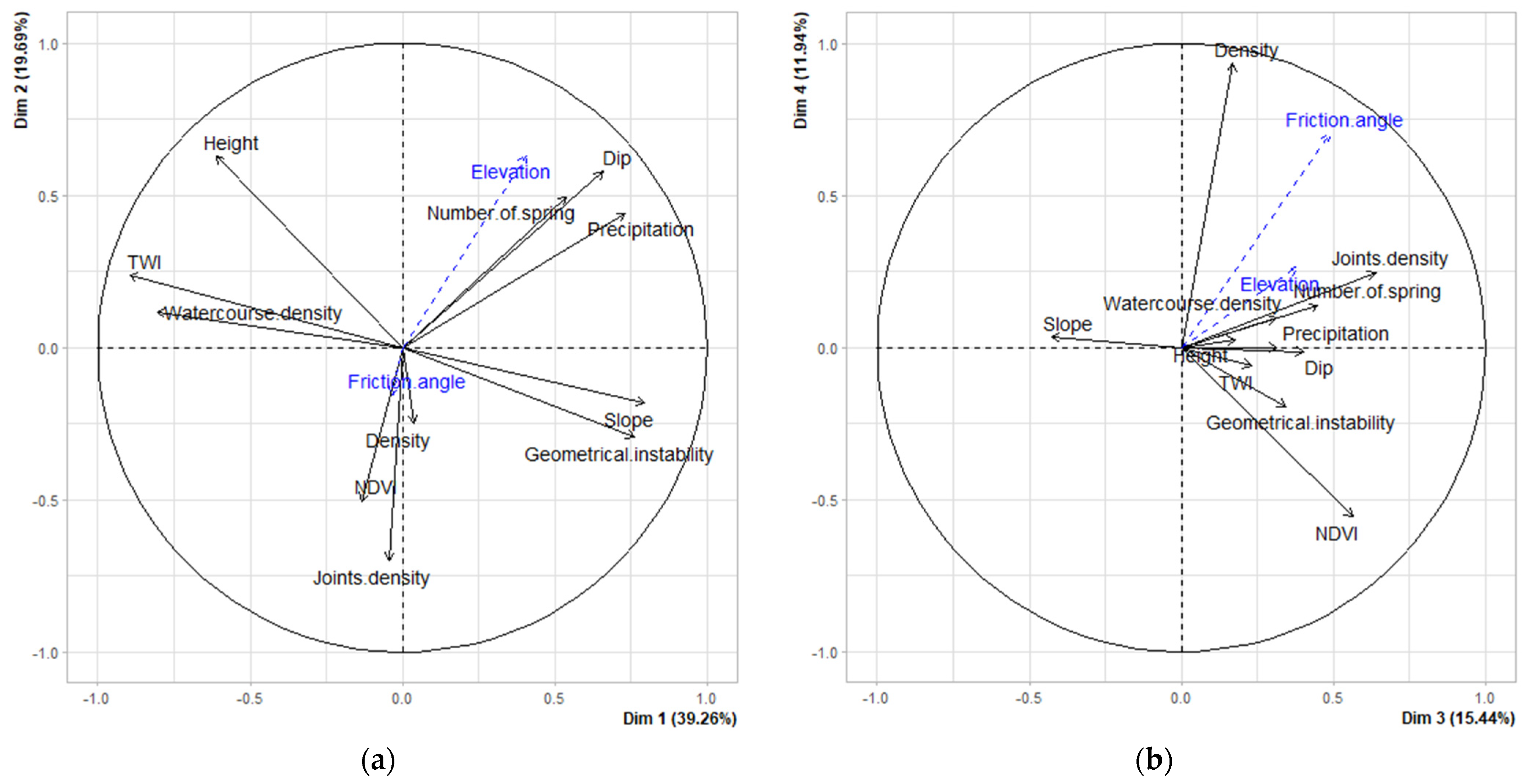
The interpretation of the graph of variables considers their average contribution on the first four axes. Only the variables whose contribution is higher than 9.09% along each axis were interpreted. According to the correlation circles (Figure 13), we notice a strong correlation between the variables “Number of springs”, “Precipitation”, and “Dip” which are positive along axis 1 and 2 and a correlation between the variables “Slope” and “Geometrical instability” which are negative along axis 1. The variable “Height” is positive along axis 1 and negative along axis 2. Similarly, the variables “TWI” and “Watercourses density” are positively correlated along axis 1. The variable “Joints density” is strongly related to axis 2. Two variables are related to axis 3, “Joints density and NDVI”, and they are orthogonal and do not show correlation. The only variable that is related to axis 4 is “Density” and it is positive along axis 4 (Figure 13).
  • Interpretation of the graph of individuals
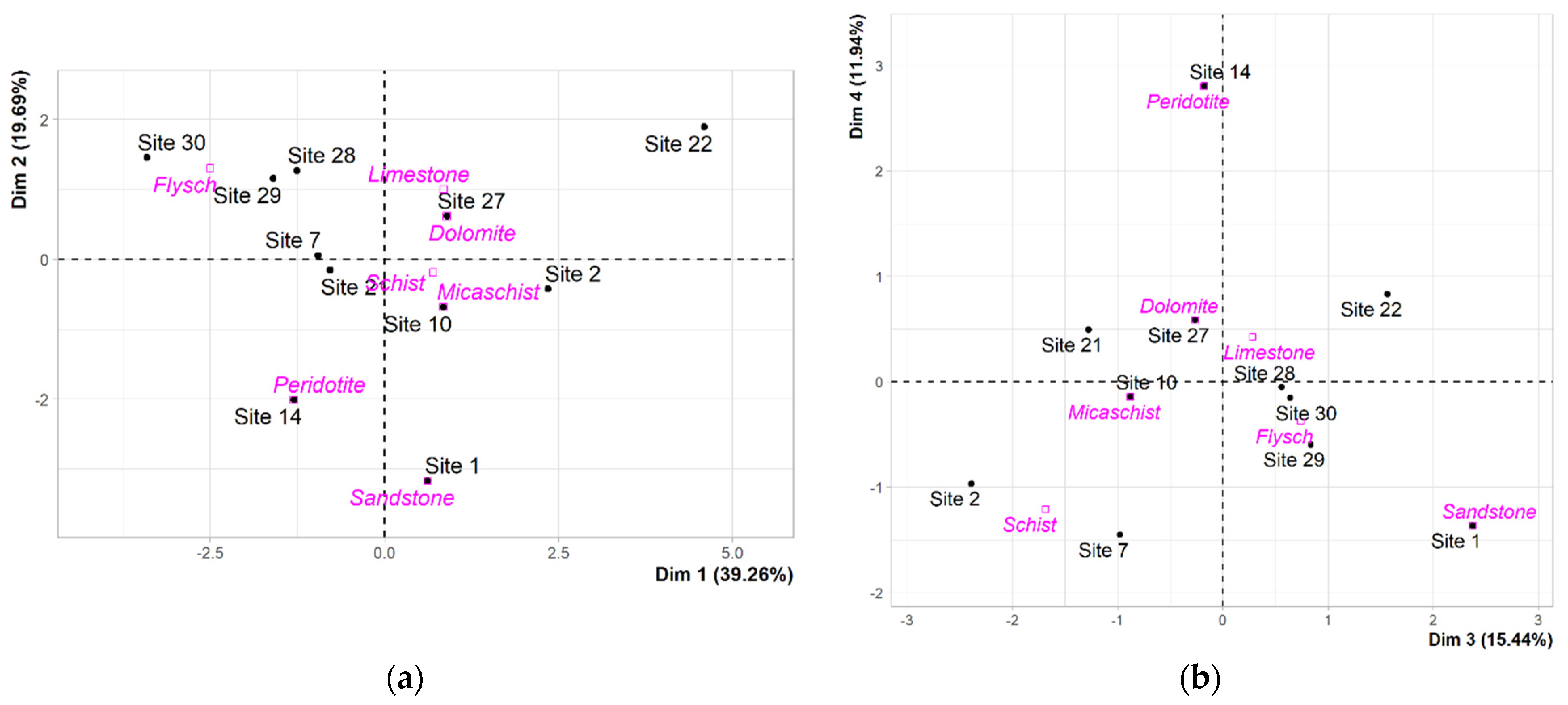
Individuals with a contribution of more than 9.09% were interpreted. Sites 2, 22, and 30 contributed strongly to the formation of the first dimension. Concerning the second dimension, site 1 alone contributed 42%. Sites 14 and 22 also contributing strongly. The sites that contributed the most to the formation of the third dimension are sites 1 and 2. The only site representative of the fourth dimension is site 14, with a contribution of 54.5%. Sites 1 and 7 also contributed but slightly (Figure 14).

4.3.3. Study of the Proximities between Points

From the graph of variables (Figure 13), the variables “Elevation”, “Precipitation”, “Number of springs”, and “Dip” are positively correlated. This is similar for the variables “TWI” and “Watercourses density” and for the variables “Slope” and “Geometrical instability”. The variables “Height”, “Density”, and “NDVI” take solitary positions in the graphs and do not show correlations with the other variables. The group of the variables consisting of TWI and Watercourses density shows a negative correlation with the group of variables consisting of Slope angle and Geometrical instability.
In the graphs of individuals (Figure 14a,b), the distribution of sites is controlled by the values of the variables. We notice that the sites form groups (subclusters) controlled by specific variables. The analysis of the contributions of the individuals according to the different axes shows that there are two types of groups of individuals: the first is homogeneous and is controlled by very specific variables. The second is heterogeneous and is controlled by several variables at the same time; in the latter, each site is independent of the others. For example, site 14 is strongly related to the fourth dimension controlled by the lithological variables (Density). Other sites have solitary positions in the graphs, namely site 1 related to “Joints density”, site 2 related to the “Slope” and “Geometrical instability” variables, and site 30 related to “Height” and “Watercourses density”. Other individuals (7, 10, 21, 27, 28, and 29) are not linked to any dimension and thus do not depend on specific variables. In this case, the variables share the same force that is applied on individuals. Similarly, site 22 is linked to several dimensions through the extreme values of the variables it presents, so it does not show a tendency towards a specific variable. In general, proximities between individuals are clearly represented along axis 1 and 2, controlled by the geological and hydrological variables, schematized by the illustrative variable “Lithology”.

4.3.4. Analysis and Interpretation of Correlations

The correlations of rockfall variables are somehow the same as for landslide variables, but some differences can be pointed out. The variable “Dip” is associated to the hydrological variables, even if no scientific evidence links the dip of a geological layer with the hydrology of the region (and vice versa). In multivariate statistical analyses, the notion of coincidence is sometimes present and must always be considered in order not to draw a wrong interpretation. Although statistical analyses show their own schematic and interpretative results, logic must always be present in these interpretations.

4.3.5. Interpretation of the Additional Qualitative Variable “Lithology”

Figure 15 visualized the study sites by the qualitative variable “Lithology”. We notice an overlap between the confidence ellipses of limestone, dolomite, schist, micaschist, and flysch. This overlap indicates that these sites have close variable values. Thus, the lithological nature of the rock may be the preponderant factor explaining rockfall susceptibility. For flysch, we notice that rockfalls are triggered in the zones of presence of fluvial terrace slopes. In statistical analysis, the area is expressed by the average values of “Watercourses density”, “TWI”, and sometimes “Height”. For sandstones, rockfalls are present most of the time in rocks having high joint density. For peridotites, the presence of rockfall is rare in the region and controlled by joint density and their persistence. As for schists, micaschists, limestones, and dolomites, we note that rockfalls are triggered by several predisposing factors that share the same global influence. In other words, each factor becomes preponderant depending on how the site is shaped.

5. Discussion

5.1. MCA

The key to the evaluation of causative factors is their contribution rate in the dataset. In principle, factors with a very low contribution value have little or no influence on the ground instabilities studied. The three factors “Spring”, “Watercourse”, and “Dip/slope” are the least influential. This conclusion is related to the variation of the modalities of the three variables with the fixed modalities of the other variables. In several study sites, we notice the repetitive aspect of certain modalities such that there is a mutual influence on one another. It is understood that in order to trigger field instability in some particular sites, it is necessary to repeat modalities. In these sites, the similarity between modalities does not concern the modalities of the three least influential variables. For example, we find that the two modalities of “Spring” variable, i.e. the presence or not of a water spring, has no effect on the modalities of the other variables. An evaluation of the most influential factors requires a more in-depth analysis. The principle is based on multiple correlation analysis, the purpose of which is to rank the variables according to the number of links that each variable has with the others. The variable having the highest number of correlations with the other variables is the most dominant in the dataset, and the variable with the least correlations is the least dominant. The analysis is realized by observing the variables whose contribution rate is more or less similar along the same factorial axis. The variables “Lithology”, “Elevation”, and “Fracture persistence” are the most dominant according to both axes 1 and 2; each of them has a correlation with eight other variables. Then, we have the variables “Slope”, “Slope exposure”, and “Climate”, with four correlations each; the variable “Anthropogenic activity”, with two correlations; and finally, just one correlation for the variables “Land use” and “Fracture opening”.
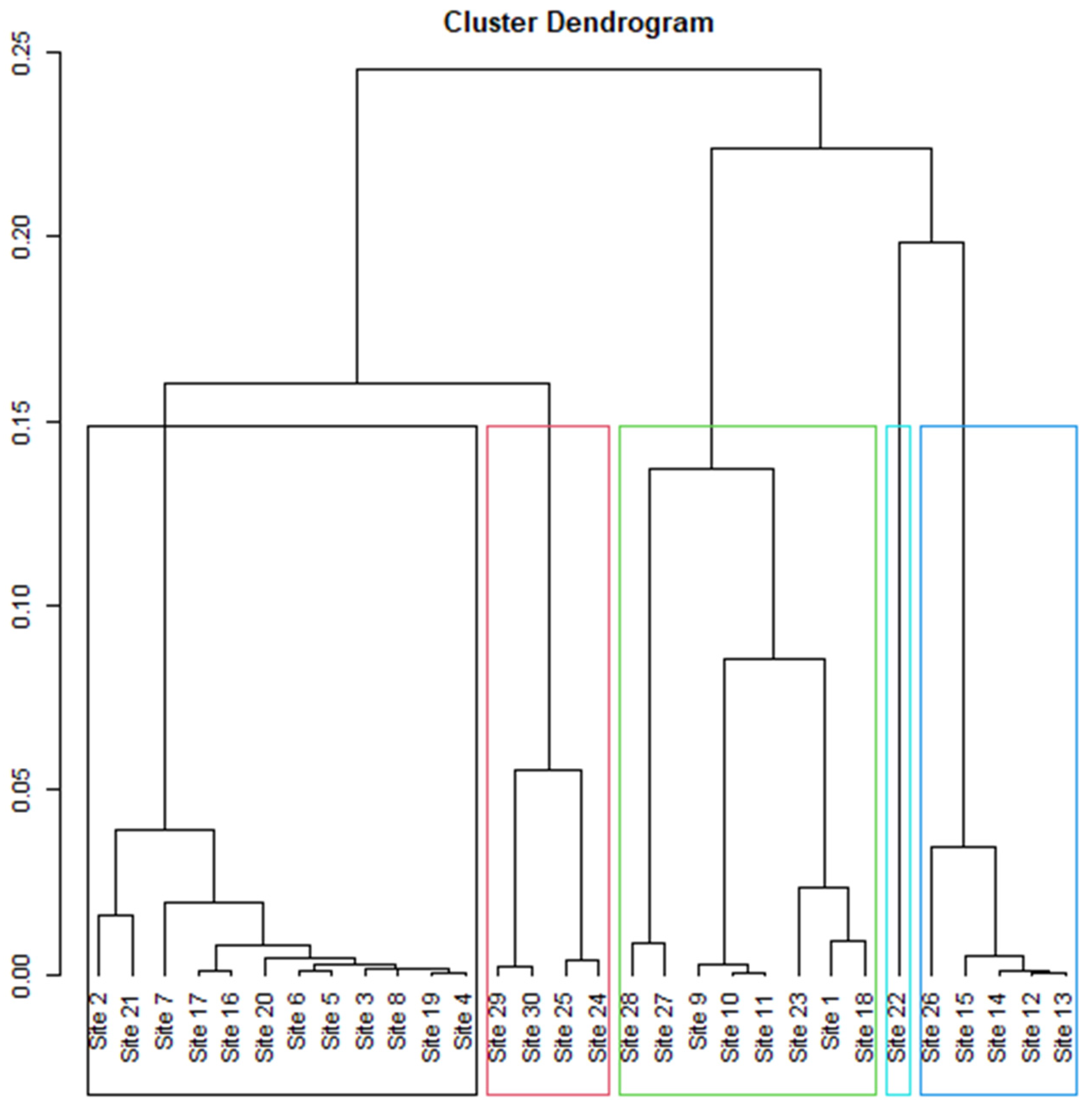
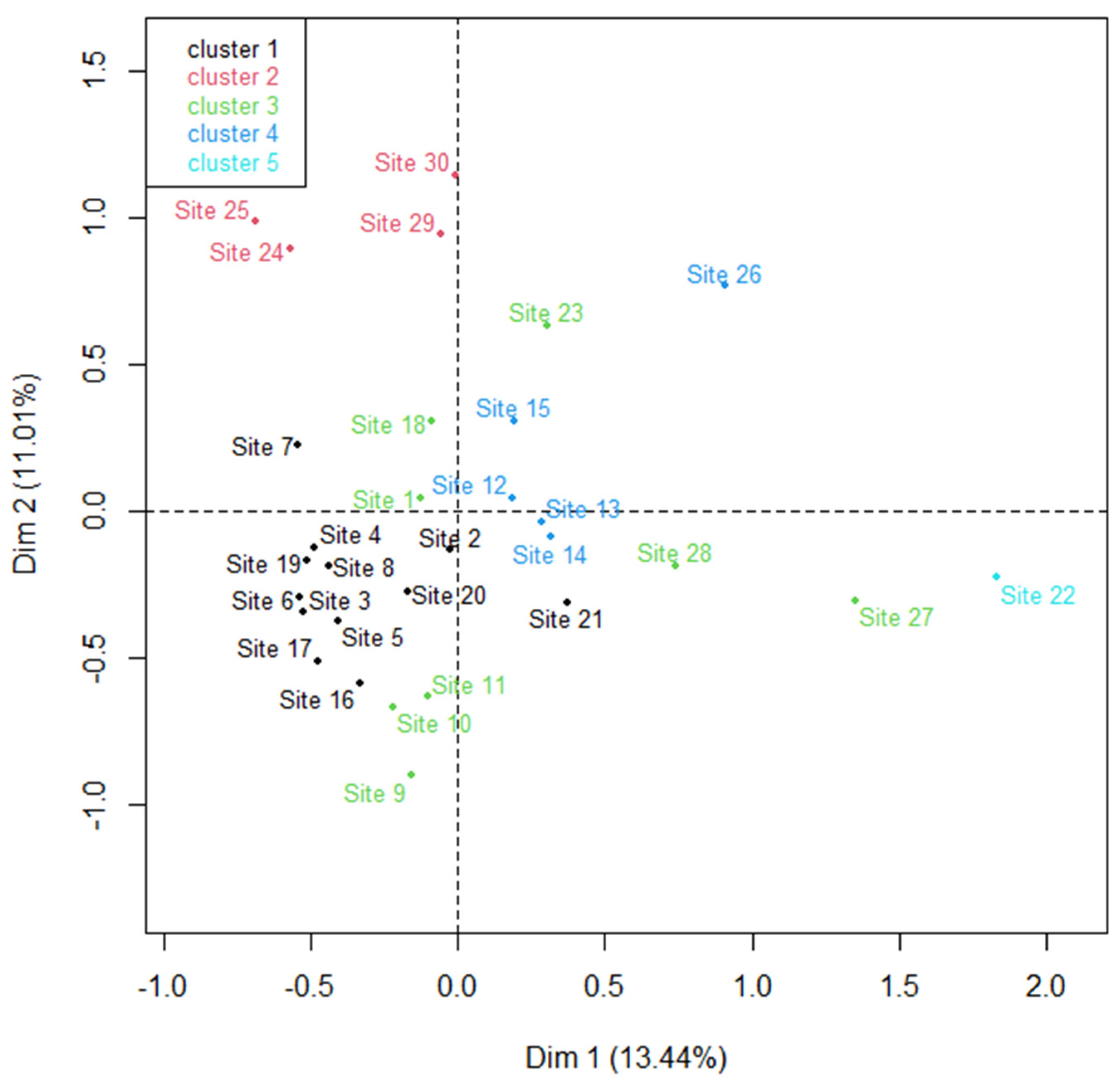
Another way of representing and analyzing multiple correlations is to perform a hierarchical classification of the data. Study sites are represented in homogeneous classes so that the sites in the same class have the same modalities of variables. Classes are distinguished by the most contributing variables. The hierarchical tree (Figure 16) obtained proposes five classes of instabilities where the discrimination between classes is globally controlled by the three variables “Lithology”, “Elevation”, and “Fracture persistence” and less by the other variables. If we superimpose the diagram of classes (Figure 17) with the graph of modalities (Figure 8), we notice that each class is represented by a type of lithology. Thus, lithology is the most significantly related factor to this classification. The modalities of the other variables can be encountered simultaneously in at least two instability classes.
From these two types of analyses, lithological factors can be ranked at the top of the pyramid of influence on instabilities in the study area, followed by fracture persistence, elevation, slope degree, slope exposure, climate, and anthropogenic activity.

5.2. PCA

5.2.1. Landslides

All active variables present in the dataset are potentially predisposing factors for landslides. Here, we seek to identify the predominant factor. By analyzing the 19 study sites through the table of site contributions to the first four dimensions, we notice that nine sites are not related to any specific variable and the others are related to at least one variable in the dataset. The fact that nine sites are not linked to any specific variable can be explained by the same influence weight of the different variables. As for sites 12, 13, and 15, we can note that they are strongly related to density and fracturing. Landslides in sites 23, 24, 25, and 26 are strongly related to the presence of water springs, which are the predominant predisposing factors. The last three remaining sites (sites 9, 16, and 20), which correspond to road slope collapse-type landslides, are strongly related to their zero NDVI and are negatively related to slope height. Site 16 is also strongly related to dip. In these three sites, anthropic interventions accentuate the natural predisposing factors to instability by weakening the mechanical parameters of the soil and the degradation of stability factors such as NDVI. Here, we can say that the total absence of vegetation is an important predisposition factor in the occurrence of landslides. In the case of site 16, in addition to the NDVI factor, the “dip of the layers” factor can have played an important role in predisposition to failure.
The study sites can be subdivided into four groups, described below, according to their predominant predisposing factors:
  • In this group, all predisposing factors in the active dataset have the same level of influence. In other words, removing or changing the value of any of the variables can completely change an unstable terrain into a stable terrain or conversely, increase the instability. Lithologically, this group includes only shales and micaschists; this may indicate that the lithological nature of the terrain controls the values of the other variables modalities. It is important to note that in the case of metamorphic rocks, schistosity most likely plays an important role, even though it is not included in the dataset because it is very difficult to quantify. Nevertheless, it can represent a very important predisposition parameter by strongly increasing the joint density and fragmenting the rock.
  • This group is represented by peridotites. It is differentiated by its high values of geomechanical parameters. In the study area, landslides are present in rocks with low to medium density except for the peridotites. Peridotites have the highest density in the area (3000 to 3200 kg/m3), and most instabilities correspond to landslides. Until further studies are undertaken, this group will be considered to be controlled by its geological parameters.
  • This group is represented by the presence of springs, which constitutes a permanent predisposition factor and is the most influential factor for landslides. It should be noted that the presence of a spring does not necessarily indicate the presence of a landslide. Similarly, the presence of a landslide near a spring does not mean that the landslide is necessarily related to this spring, and this has been proven by the PCA.
  • This group includes the majority of landslides encountered in the vicinity of an anthropogenic infrastructure (road, runway, structure, etc.). Man can intervene and modify certain natural parameters, in particular geomechanical parameters and the NDVI of the terrain, and thus increase the susceptibility of landslides. According to PCA, this group is controlled by NDVI, which has a negative value most of the time, thus decreasing the stability. Moreover, the negative value of NDVI becomes an indicator that the area where the landslide is located has been affected by anthropogenic interventions.
Variables in the dataset can therefore be classified according to their order of influence on landslides in the study area. According to the analysis of the four groups, the lithological nature of the terrain is preponderant, even though it is represented by a single active variable, “Density”. The fact that the first group, whose variables share the same rate of influence, is represented only by shales and micaschists, is a strong indication that lithology plays a primary role in this mechanism. The same is true for the second and fourth groups. Springs are ranked second in importance and are strongly responsible for many landslides regardless of lithologic nature and other terrain parameters. Vegetation density is ranked third in order of importance, due to low values at all of the sites and, most relevantly, at the anthropized sites. The density of mechanical discontinuities and the dip of the layers come fourth, as very few landslides are directly related to these two parameters. Rather, it is the orientation of these two parameters in relation to the slope that determines whether they have an influence or not. The density of the hydrographic network and the topographic wetness index have very low basic values and can be classified as the least influential in fifth order. For the geometric parameters (Slope and Height), the sites did not show strong positive contributions towards these two parameters. In our case, geometric parameters can be considered to be indispensable preparation factors and not as predisposing factors, and a minimum value is, in any case, required to induce a failure.

5.2.2. Rockfalls

As with landslides, we seek to identify the overriding factors responsible for landslides. By analyzing the 11 study sites through the table of site contributions to the first four dimensions, we notice that some sites are related to well-defined variables, which provides an idea about the corresponding location where a rockfall occurred or could occur. Sites 28, 29, and 30 are characterized by a high slope height and a moderately dense drainage network. These parameters indicate a favorable location for triggering or encountering a rockfall. This often corresponds to a large valley crossed by a mainstream. The phenomenon of solifluction, strongly present in these places, dragging a large mass of sediments down the slope, digs up the underlying rocks in places and lets them outcrop on the surface. The outcropped rocks are then exposed to instability factors, making them susceptible to tumbling at any time. Other valleys are morphologically similar to these, but have parameters that slow down the processes of soil solifluction, which explains the absence of this type of rockfall. Site 14 presents a case of rockfall triggered in peridotitic massif. It is encountered exclusively at the level of upstream slopes where the highly fractured rock outcrops form a rocky escarpment with a steep slope and scarce vegetation. According to the graph of individuals, site 1 has the highest joint density, significant vegetation, and a high number of geometrical instabilities. The slump zone corresponds to a road slope where vegetation is absent, even though data indicate a high presence of vegetation (calculation by magnitude zone). High joint density contributed to a high number of geometric instabilities, making this area favorable to rockfalls at a high frequency. Site 22 is characterized by a subvertical slope, very steep dip, high altitude and interannual precipitation, and many potential geometrical instabilities. In the study area, the only location that encompasses all these features corresponds to carbonate bars located at the crests of slopes, whose occurrence is related to large thrusts. Here, the rockfalls are in no way related to the presence of springs located below the detachment zone, which justifies the deletion of the factor “Number of springs” to improve the readability of the results. Site 2 is characterized by its slope which exceeds 90° through the phenomenon of undercutting favored by marine erosion. Although the density of fracturing is very low at these locations, it is sufficient to have a geometrical instability to have a susceptibility to rockfall. It is obvious that rockfalls in these locations are rare and have a very low frequency. The four remaining sites (7, 10, 21, 27) are not linked to a specific factor, which can be explained by the fact that the different factors share the same influence weight on the site. On the other hand, for each rockfall movement, one of the factors can be preponderant without forgetting to privilege the factors (slopes and joint density) essential to the movement.
From the analysis of the study sites, we find that the factors “Slope” and “Joints density” are the most influential on rockfall movements. We find that 80% of the sites have slopes steeper than 60°. The number of geometric instabilities and the density of the hydrographic network come second. In some sites, the high number of geometrical instabilities was a necessary predisposing element for the movement. Likewise, the increase in the number of geometric instabilities has an influence on the increase in the frequency of rockfalls. The presence of a high density of the hydrographic network at the level of narrow valleys of the study area favors the outcrop of rocks at the surface and exposes them to aggravating factors. In addition, the hydrographic network plays a secondary role in eroding the lower slope support (toe stop). It generates landslides where the slid mass plays a supporting role for the rock mass. Some variables such as “NDVI” and “TWI” show almost similar values for all sites. Our interpretation of the low values of “NDVI” is that rockfall movements all occurred in areas with very low density of vegetation. It shows that the presence or absence of vegetation plays an important part in the process. Here, PCA does not have the ability to show some recovery of sites to variables with nearly similar values. The same applies to TWI, which shows low values indicating slumping in steep slopes areas. The dip of the layers is the least influential parameter on rockfall due to its low values. The variation of the slope height does not influence rockfall movements, except in the case of flysch, where a significant slope height is required to have rockfall susceptibility. Varying the values of the last three remaining factors (Number of springs, Precipitation and Density) showed no direct influence on rockfalls.
In the case of rockfalls, we have noticed that, in general, the variables rarely have extreme values. The most important parameters in rockfalls are geometric (Slope and Exposure) and structural (Joint density and Geometrical instability) parameters. In contrast to landslides, geotechnical parameters do not show a great influence on landslides, rather they show an indirect influence in shaping the morphological elements of the terrain and the internal structuring of the soil. Moreover, rockfalls are found in the different lithology types, perhaps not with the same frequency, but movement is ubiquitous regardless of the geotechnical parameters of the rock.

5.3. Synthesis of Causative Factors

The final assessment of the causative factors is established via the combination of the MCA and PCA results. We point out once again that field instabilities are encountered at the level of the different modalities of causative factors and that instabilities can be triggered by several combinations of modalities. The fact of modifying a modality in a combination can make a terrain stable indicates that it is important to know the weight of the influence of each causative factor and its real effect on the study site. Here, the aim is not to observe the degree of influence of each factor on the study area, but rather to examine the influence of each factor on the other in relation to the ground instabilities studied, so as to say for each site which was the determining and indispensable parameter to make the ground instability appear. From interpretations of the two methods, the lithological factors can be considered as the most influential on ground instabilities. This is related to MCA and the landslide part of PCA which rank lithological variables at the top of the influence pyramid, a little less in the PCA rockfall part. This shows that lithology has an influence on several parameters, notably the geometrical and structural parameters. Globally, ground instabilities, as far as carbonate rocks are concerned, are present in high altitudes, steep slopes, in terrain with high fractures persistence and high joint density, etc. This is different for instabilities located in the schists, presenting average slopes, weak altitudes, less dense and less persistent fractures, etc. This emphasizes that lithology is an important element in determining the existing classes of instabilities. Structural factors, persistence and joint density, come in second place. These factors determine the extent of the instabilities represented by their size and frequency. In some sites, the high joint density increases the chance of having geometric instability; in other sites, it is rather the persistence of the discontinuities which generates geometric instability in places. The influence of geometrical factors on instability comes third. We note that the slope is much more important in rockfalls than in landslides. The slope represents a primordial element in the instabilities studied, as a minimal value is always required. Hydrological factors come fourth. The sites related to these factors are completely independent from the other sites, because hydrological entities are the determining parameters of existing instabilities. The ranking of these factors is linked to the low values of hydrographic densities and the absence of springs in most of the sites. Anthropogenic factors, the type and density of vegetation, and land use come last and are factors that influence the acceleration of instabilities. They are factors that amplify the previous instability factors.

5.4. Reproductibility of the Methodoly

An extensive ground instability inventory is the first essential step for such an analysis. It allows the efficiency and fast selection of representative study sites (with existing ground instabilities) that are used for causative factors analysis. If such an inventory is inaccessible or inaccurate, we strongly recommend realizing one following the methodology described in [19]. Indeed, without such an inventory, randomly chosen study sites may not be well representative of the study area. This will affect the quality of the results and thus can lead to less accurate results. Similarly, the descriptive data of the inventory should be as comprehensive as possible. To obtain relevant results, ongoing feedback with the study sites must be obtained in order to take into account their specificities and complexities. This is all the more important depending on the causative factors that should be taken into account, as the causative factors depend strongly on the studied areas.

6. Conclusions

This study showed that multivariate statistical analyses are appropriate methods for evaluating causative factors. They can be descriptive or explanatory depending on the objective sought. In our study, the analysis of causative factors required the processing of qualitative and quantitative data. MCA was used for qualitative variables and PCA was used for quantitative variables. We were able to point out that:
  • The choice of factorial designs depends on the terminology of the study and of the objectives sought.
  • For an analysis to be fair and complete, the dimensions chosen must be representative of the causative factors, and each factor must have a minimum contribution.
  • For both methods (MCA and PCA), multiple correlation analysis highlighted the number of interrelationships for each factor.
  • In MCA, the classification of factors according to their order of influence can be performed through the observation of the number of correlations of each factor and through a hierarchical classification that groups the study sites into instability classes.
  • In PCA, the assessment of influence degree causative factors depends on the correlations number analysis between variables, and even more on the belonging of the study sites to a specific group of variables.
In the coastal region between Tetouan and Jebha, statistical analyses considered geological factors to be the most influential on ground instabilities, followed by geometric, climatic, hydrological, environmental (vegetation and land use), and anthropogenic factors. The analysis also showed that the type and frequency of instability are intrinsic to the influence weight of each causative factor.
Finally, it is important to point out that an expert’s judgement remains indispensable in multivariate statistical analysis, especially in PCA. An expert’s role is essential when the modalities of the variables present extreme values and when individuals do not show a visible trend for one or more specific variables. Vigilance is required regarding the interpretation of correlations, as statistical methods can sometimes show correlations that have no logical interpretation.

Author Contributions

Conceptualization, H.T., M.G.-B. and A.E.G.; methodology, H.T. and M.G.-B.; software, H.T.; validation, H.T., M.G.-B. and A.E.G.; formal analysis, H.T.; investigation, H.T.; resources, H.T.; data curation, H.T.; writing—original draft preparation, H.T.; writing—review and editing, H.T. and M.G.-B.; visualization, H.T.; supervision, M.G.-B. and A.E.G.; funding acquisition, H.T. All authors have read and agreed to the published version of the manuscript.

Funding

This research received no external funding.

Data Availability Statement

Data will be available upon request.

Conflicts of Interest

The authors declare no conflict of interest.

Appendix A. Imput data for MCA and PCA

Table A1. MCA input data. See explanation of the abbreviations in Table 1.
Individual
Variable
TypeLithologyBinderPersistenceFracture OpeningFracture FillingFracture Distrib.Dip/
Slope
SlopeElevationExposureWater SourceSpringLand UseAnthropologic ActivityClimate
Site 1CSdQMin/MedJointedMinz.Prevail.Out.Steep0–200EAAMatorralRoadS H
Site 2RSClMed/MajOpenCloggedEquiv.Out.V steep0–200EAAForestUnaffectedS H
Site 3LSClMedOpenCloggedEquiv.Ent.Slight0–200NAPMatorralRoadS H
Site 4LSClMedOpenCloggedPrevail.Out.Slight0–200NPPMatorralRoadS H
Site 5LSClMedOpenCloggedEquiv.Out.Steep0–200NPPMatorralRoadS H
Site 6LSClMedOpenCloggedEquiv.Out.Slight0–200EAAMatorralRoadS H
Site 7RSClMedOpenCloggedPrevail.Ent.Slight0–200EAAUrb areaDwellingsS H
Site 8LSClMedOpenCloggedPrevail.Ent.Slight0–200NPAMatorralRoadS H
Site 9CMSQ-MMedJointedMinz.Equiv.Out.Steep0–200NAAExposedRoadS H
Site 10RMSQ-MMedJointedMinz.Equiv.Ent.Steep0–200EAAMatorralRoadS H
Site 11LMSQ-ClMedJointedMinz.Prevail.Out.Steep0–200EAAExposedRoadS H
Site 12LPNoneMed/MajOpenMinz.Prevail.Out.Slight0–200EAAForestRoadS A
Site 13LPNoneMed/MajOpenMinz.Prevail.Out.Steep0–200EAAForestRoadS A
Site 14RPNoneMed/MajOpenMinz.Prevail.Out.Steep0–200NPAForestRoadS A
Site 15LPNoneMed/MajOpenMinz.Prevail.Ent.Slight0–200EPAMatorralDwellingsS A
Site 16CMSClMedOpenCloggedEquiv.Out.Slight0–200NAPExposedRoadS A
Site 17LMSClMedOpenCloggedEquiv.Out.Slight0–200NAAMatorralRoadS A
Site 18LSClMin/MedJointedMinz.Prevail.Out.Gentle0–200WPAMatorralRoadArid
Site 19CSClMediumOpenCloggedPrevail.Out.Slight0–200NAPMatorralRoadArid
Site 20LSClMed/MajOpenCloggedPrevail.Out.Slight0–200NAAExposedRoadArid
Site 21RLCaMed/MajOpen/JointedCloggedPrevail.Out.Steep0–200NAAMatorralUnaffectedArid
Site 22RLCaMed/MajOpenMinz.Prevail.Ent.Steep900–1100SAPExposedUnaffectedV H
Site 23LSdQMin/MedJointedMinz.Prevail.Out.Gentle600–800WAPMatorralRoadH
Site 24LSClMin/MedOpenCloggedPrevail.Out.Gentle200–400EAAMatorralDwellingsS H
Site 25LSClMin/MedOpenCloggedPrevail.Out.Gentle200–400NAPUrb areaDwellingsS H
Site 26LPNoneMed/MajOpenMinz.Prevail.Ent.Slight400–600SPPForestDwellingsHumid
Site 27RLCaMed/MajOpenMinz.Equiv.Out.Steep900–1100WPAExposedUnaffectedHumid
Site 28RDCaMed/MajOpenMinz.Equiv.Out.Slight600–800WPAExposedUnaffectedS H
Site 29RFCl-LMin/MedOpenCloggedPrevail.Out.Slight400–600EAPMatorralUnaffectedS A
Site 30LFCl-LMin/MedOpenCloggedPrevail.Out.Gentle400–600EPAMatorralUnaffectedS A
Table A2. PCA landslide input data. See explanation of the abbreviations in Table 2.
IndividualLandslide
Depth
LithologyΦ
(°)
C
(kPa)
Density
(kg/m3)
Dip
(°)
Joint Density
(m−3)
Precipitation
(mm/an)
Slope Angle
(°)
Height
(m)
Elevation
(m)
Watercourse
(m−2)
Nb of SpringsNDVITWI
Site 3DeepSchist155002300202.5600502001500.76510.15.78
Site 4ShallowSchist152502300203.5600501002000.76520.16.5
Site 5ShallowSchist152802300253.5600551002500.58410.066.5
Site 6DeepSchist151352300152.46004580300.58400.028.5
Site 8DeepSchist154302300157.66600452001500.76500.025.78
Site 9ShallowMicaschist15702500107.286006525901.980−0.255.78
Site 11ShallowMicaschist157702500407.28600602501600.76500.026.5
Site 12ShallowPeridotite301403200013.5400501201500.3700.075.2
Site 13ShallowPeridotite302603200013.5400651201500.3700.073.5
Site 15ShallowPeridotite301203200013.5400451502000.76500.038
Site 16ShallowMicaschist154002500657.24400501701700.5841−0.255.78
Site 17ShallowMicaschist156702500457.24400502502200.58400.055.2
Site 18ShallowSchist151352300157.2440040701751.35500.013.5
Site 19DeepSchist1532023004012.24400451601001.35510.025.78
Site 20ShallowSchist15250230015440050100302.85500.022.5
Site 23DeepSandstone259025001016900321207001.9820.128
Site 24DeepSandstone2520025002014.5700352003501.56210.26.5
Site 25ShallowSchist1518023001010.5700401003000.95520.128.5
Site 26ShallowPeridotite302503200013.5900521507001.9830.027.5
Table A3. PCA rockfall input data. See explanation of the abbreviations in Table 2.
IndividualLithologyΦ
(°)
Density
(kg/m3)
Dip
(°)
Joints
Density
(m−3)
Geometric
Instability
Precipitation
(mm/an)
Slope Angle
(°)
Height
(m)
Elevation
(m)
Watercourse DensitySpringNDVITWI
Site 1Sandstone252500251856006012550.76500.23.5
Site 2Schist152300303.53600110105000.022
Site 7Schist15230010316005040800.58400.085.2
Site 10Micaschist152500158.28460080851500.3700.023.2
Site 14Peridotite303200013.514006540901.35500.024.6
Site 21Limestone252600207.50400601001000.3700.023.5
Site 22Limestone252700807.665110085451100020.012.2
Site 27Dolomite252700356.52900609010500.3700.023.2
Site 28Limestone252600407.220700452007000.76500.084.6
Site 29Flysch202400257.221500501654501.35510.085.78
Site 30Flysch202400257.221500401752002.85500.027.5

References

  1. Petley, D. Global patterns of loss of life from landslides. Geology 2012, 40, 927–930. [Google Scholar] [CrossRef]
  2. Froude, M.J.; Petley, D. Global fatal landslide occurrence from 2004 to 2016. Nat. Hazards Earth Syst. Sci. 2018, 18, 2161–2181. [Google Scholar] [CrossRef] [Green Version]
  3. Guzzetti, F.; Mondini, A.C.; Cardinali, M.; Fiorucci, F.; Santangelo, M.; Chang, K.T. Landslide inventory maps: New tools for an old problem. Earth Sci. Rev. 2012, 112, 42–66. [Google Scholar] [CrossRef] [Green Version]
  4. Capecchi, V.; Perna, M.; Crisci, A. Statistical modelling of rainfall-induced shallow landsliding using static predictors and numerical weather predictions: Preliminary results. Nat. Hazards Earth Syst. Sci. 2015, 15, 75–95. [Google Scholar] [CrossRef] [Green Version]
  5. Guzzetti, F.; Ardizzone, F.; Cardinali, M.; Galli, M.; Reichenbach, P.; Rossi, M. Distribution of landslides in the Upper Tiber River basin, central Italy. Geomorphology 2008, 96, 105–122. [Google Scholar] [CrossRef]
  6. Martins-Campina, B. Le Rôle des Facteurs Géologiques et Mécaniques dans le Déclenchement des Instabilités Gravitaires: Exemple de Deux Glissements de Terrain des Pyrénées Atlantique (Vallée d’Ossau et Vallée d’Aspe). Ph.D. Thesis, Planète et Univers, Université Bordeaux I, Bordeaux, France, 2005. [Google Scholar]
  7. Tang, Y.; Feng, F.; Guo, Z.; Feng, W.; Li, Z.; Wang, J.; Sun, Q.; Ma, H.; Li, Y. Integrating principal component analysis with statistically-based models for analysis of causal factors and landslide susceptibility mapping: A comparative study from the loess plateau area in Shanxi (China). J. Clean. Prod. 2020, 277, 124–159. [Google Scholar] [CrossRef]
  8. Gasc-Barbier, M.; Virely, D.; Guittard, J.; Merrien-Soukatchoff, V. Different approaches to fracturation of mable rock—The case study of the St Beat tunnel (French Pyrenees). In Proceedings of the International Society for Rock Mechanics, Liege, Belgium, 9–12 May 2006; pp. 619–623. [Google Scholar]
  9. Delonca, A.; Gunzburger, Y.; Verdel, T. Statistical correlation between meteorological and rockfall databases. Nat. Hazards Earth Syst. Sci. 2014, 14, 1953–1964. [Google Scholar] [CrossRef] [Green Version]
  10. Jebur, M.N.; Pradhan, B.; Tehrany, M.S. Optimization of landslide conditioning factors using very high-resolution airborne laser scanning (LiDAR) data at catchment scale. Remote Sens. Environ. 2014, 152, 150–165. [Google Scholar] [CrossRef]
  11. Liu, Y.; Zhang, W.; Zhang, Z.; Xu, Q.; Li, W. Risk factor detection and landslide susceptibility mapping using Geo-Detector and Random Forest Models: The 2018 Hokkaido eastern Iburi earthquake. Remote Sens. 2021, 13, 1157. [Google Scholar] [CrossRef]
  12. Leroi, E.; Favre, J.L.; Rezig, S. Cartographie de l’aléa mouvements de terrain par analyse statistique sous SIG. Rev. Fr. De Géotech. 2001, 95–96, 155–163. [Google Scholar] [CrossRef]
  13. El Fellah, B.; Mastere, M. The central Rif Mediterranean coast: Slope failures causative factors. Bull. De L’institut Sci. 2015, 37, 35–43. [Google Scholar]
  14. Andrieux, J. La structure du Rif central. Etude des relations entre la tectonique de compression et les nappes de glissement dans un tronçon de la chaîne alpine. Notes Et Mémoires Du Serv. Géologique Du Maroc 1971, 235, 1–450. [Google Scholar]
  15. Kornprobst, J. Contribution à l’étude pétrographique et structurale de la zone interne du Rif (Maroc septentrional). Notes Et Mémoires Du Serv. Géologique Du Maroc 1974, 256, 1–251. [Google Scholar]
  16. Chalouan, A.; Michard, A. The Alpine Rif Belt (Morocco): A case of mountain building in a subduction-subduction-transform fault triple junction. Pure Appl. Geophys. 2004, 16, 489–519. [Google Scholar] [CrossRef]
  17. Michard, A.; Negro, F.; Saddiqi, O.; Bouybaouene, M.L.; Chalouan, A.; Montigny, R.; Goffé, B. Pressure–temperature–time constraints on the Maghrebide mountain building: Evidence from the Rif–Betic transect (Morocco, Spain), Algerian correlations, and geodynamic implications. Comptes Rendus Geosci. 2006, 338, 92–114. [Google Scholar] [CrossRef]
  18. Afiri, A. Etude Pétro-Structurale des Péridotites de Béni Bousera et des Roches Crustales sus-Jacentes (Rif Interne, Maroc): Implications Géodynamiques. Ph.D. Thesis, Pétrologie Métamorphique et Structurale, Université Cadi Ayyad, Marrakech, Morocco, 2011. [Google Scholar]
  19. Tribak, H.; Gasc-Barbier, M.; El Garouani, A. A multi-temporal ground instabilities inventory between Tetouan and Jebha (Morocco): Mapping, description and analysis. Bull. Eng. Geol. Environ. under review.
  20. Husson, F.; Josse, J. Multiple Correspondence Analysis. In Visualization and Verbalization of Data, 1st ed.; Blasius, J., Greenacre, M., Eds.; Chapman and Hall: New York, NY, USA, 2014; 392p. [Google Scholar] [CrossRef]
  21. Guerrien, M. L’intérêt de l’analyse en composantes principales (ACP) pour la recherche en sciences sociales. Cah Des Amériques Lat. 2003, 43, 181–192. [Google Scholar] [CrossRef]
  22. Lê, S.; Josse, J.; Husson, F. FactoMineR: An R package for multivariate analysis. J. Stat. Softw. 2008, 25, 1–18. [Google Scholar] [CrossRef] [Green Version]
  23. Itasca. Available online: https://www.itasca.fr/en/software/flac-slope (accessed on 30 August 2022).
  24. Gasc-Barbier, M.; Merrien-Soukatchoff, V.; Virely, D. The role of natural thermal cycles on a limestone cliff mechanical behavior. Eng. Geol. 2021, 293, 106293. [Google Scholar] [CrossRef]
  25. Gasc-Barbier, M.; Ballion, A.; Virely, D. Design of large cuttings in jointed rock. Bull. Eng. Geol. Environ. 2008, 67, 227–235. [Google Scholar] [CrossRef]
  26. Braeken, J.; van Assen, M.A.L.M. An empirical Kaiser criterion. Psychol. Methods 2017, 22, 450–466. [Google Scholar] [CrossRef] [Green Version]
  27. Mbacké Dia, C.A.K.; Sarr, A.G.R.J.; Kafom, A.; Diome, T.; Ngom, D.; Thiaw, C.; Ndiaye, S.; Sembene, M. Identification morphométrique despopulations de Tribolium castaneum Herbst (Coleoptera, Tenebrionidae) inféodées à trois céréales à WidouThiengoli. J. App. Biosci. 2017, 119, 11929–11942. [Google Scholar] [CrossRef]
  28. Baccini, A. Statistique Descriptive Multidimensionnelle (pour les nuls). Publications de l’Institut de Mathématiques de Toulouse 2010. Available online: https://math.univ-toulouse.fr/~baccini/zpedago/asdm.pdf (accessed on 30 August 2022).
  29. Husson, F.; Lê, S.; Pagès, J. Analyse de Données Avec R; Presses Universitaires de Rennes: Rennes, France, 2009; p. 238. [Google Scholar]
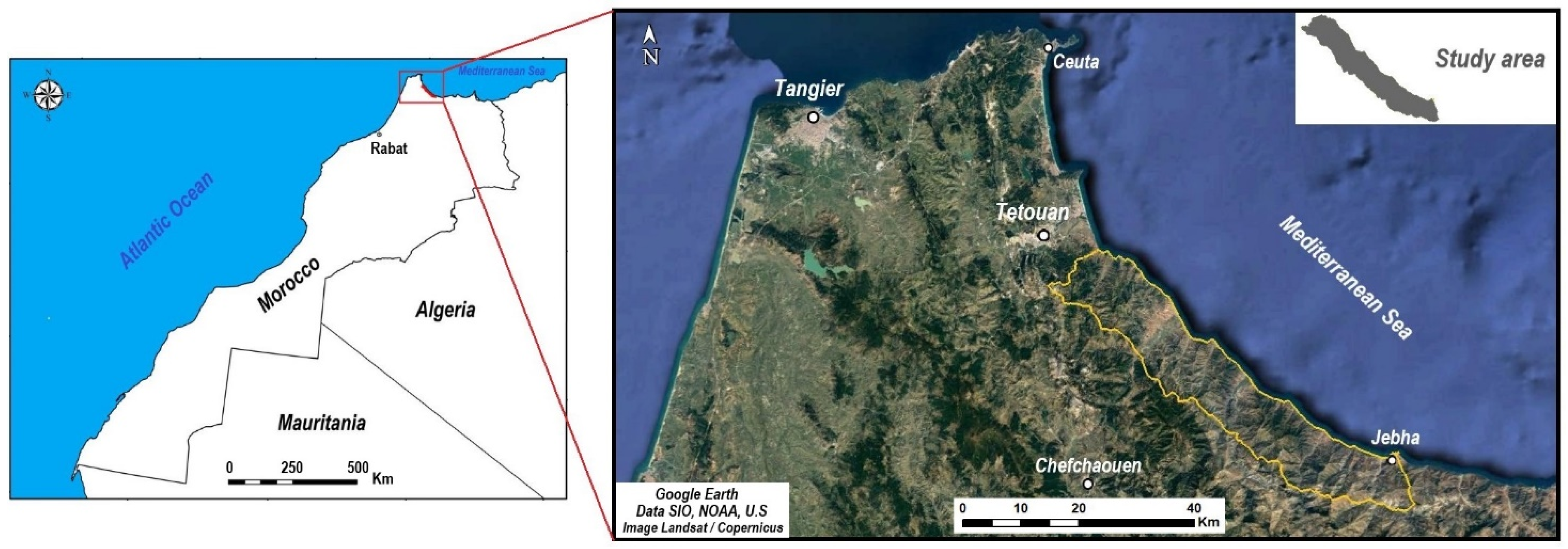
Figure 1. Geographical location of the study area (within the yellow line).
Geosciences 12 00383 g001
Figure 2. Geological map of the northwestern Rif [18] (modified). The area is surrounded in red.
Geosciences 12 00383 g002
Figure 3. Ground instability inventory map of the area [19]. (a, b, c, d correspond to Figure 4).
Geosciences 12 00383 g003
Figure 4. Examples of ground instability types in the study area. (a) Rockfall in a limestone cliff. (b) Road slope collapse. (c) Gullies formation in a valley slope. (d) Landslide in peridotites.
Geosciences 12 00383 g004
Figure 5. Distribution map of the study sites.
Geosciences 12 00383 g005
Figure 6. MCA total inertia decomposition.
Geosciences 12 00383 g006
Figure 7. Graph of MCA variables.
Geosciences 12 00383 g007
Figure 8. Graph of MCA modalities.
Geosciences 12 00383 g008
Figure 9. The total inertia decomposition of landslide PCA.
Geosciences 12 00383 g009
Figure 10. Graph of individuals. (a) According to axes 1 and 2; (b) according to axes 3 and 4.
Geosciences 12 00383 g010
Figure 11. Correlation variables circle, landslide PCA. Along (a) axis 1 and 2; (b) axis 3 and 4.
Geosciences 12 00383 g011
Figure 12. The total inertia decomposition of PCA rockfall.
Geosciences 12 00383 g012
Figure 13. Correlation circle of variables. Rockfall PCA - along (a) axis 1 and 2; (b) axis 3 and 4.
Geosciences 12 00383 g013
Figure 14. Graph of individuals. (a) According to axis 1 and 2; (b) according to axis 3 and 4.
Geosciences 12 00383 g014
Figure 15. Representation of the study sites according to “Lithology”.
Geosciences 12 00383 g015
Figure 16. Hierarchical tree of instability classes. Each color is a different cluster (see Figure 17).
Geosciences 12 00383 g016
Figure 17. Representation of the study sites according to their class.
Geosciences 12 00383 g017
Table 1. Definition of the MCA variables, also used in Appendix A (Table A1).
VariableDefinition
TypeThree types of ground movements were considered:
Landslides (L): all varieties of landslides were considered except for mudflows
Rockfalls (R): only rockfall larger than 10 m3 were considered
Road slope collapse (C): mass movements generated in artificial slope
LithologySd: sandstone, S: schist, MS: micaschist, P: peridotite, L: limestone, D: dolomite, F: flysh
BinderNature of the cement or matrix interposed between the lamination joints (Q: quartzitic, Cl: claystone, M: mica, Ca: calcite, L: limestone)
Fracture persistenceMinor: not exceeding the thickness of the bank and/or length < 1 m
Medium: crossing several banks and/or 1 m < length < 10 m
Major: 10 to 100 m long
Fracture fillingMineralized (Minz.): minerals of one or more visible generations
Clogged: diffuse and homogeneous filling
Fracture openingSpecifies whether the fractures are open or joined
Fracture distributionEqui. (Equivalent system): homogeneous fracture network with a grid distribution
Prev. (Prevailing system): heterogeneous fracture network with a random organization
Dip/SlopeEnt (Entering): layers are opposite to the slope
Out (Outgoing): layers are in the same direction as the slope
SlopeGentle: slope less than 45°
Slight: slope between 45 and 55°
Steep: slope between 55 and 90°
Very steep: slope greater than 90°
ElevationRepresented in the analysis by classes to appear as qualitative data
ExposureExposure of the slopes according to cardinal points: N (north), S (south), E (east), W (west)
WatercoursePresence: the ground movement is in intersection with one of the morphological components of a watercourse
Absence: total absence of watercourses in the vicinity of the movement.
(Water) SpringPresence: spring within 10 m of the center of the movement
Absence: total absence of spring near the movement
Anthropogenic activityRoad: presence of a road within a maximum distance of 5 m
Dwellings: presence of a dwelling beyond maximum distance of 20 m
Unaffected: absence of anthropogenic factors in the vicinity of the movement
Table 2. Definition of the PCA variables also used in Appendix A (Table A2 and Table A3).
VariableDefinition
Φ (°)Friction angle
C (kPa)Cohesion
Density (kg/m3)Density of the intact rock
Joint densityDensity of mechanical discontinuities: corresponds to the number of mechanical discontinuities/m3.
Estimated from the analysis of fracture families and stratification banks
Precipitation (mm/an)Precipitation rates for the last 5 years
Height (m)Height of the slope where the ground movement is located
Elevation (m)Average elevation level where the lower part of the movement is located
Density of the hydrographic networkCorrespond to the number of watercourses/m2. Calculated from a GIS analysis that classifies rivers into magnitude zones
NDVINormalized differential vegetation index
TWITopographic wetness index
Geometric instabilityNumber of geometric instabilities (dihedrals or plane slides) obtained with a typical stereographic stability analysis
Publisher’s Note: MDPI stays neutral with regard to jurisdictional claims in published maps and institutional affiliations.