The Evolution of the Two Largest Tropical Ice Masses since the 1980s

Abstract

As tropical glaciers continue to retreat, we need accurate knowledge about where they are located, how large they are, and their retreat rates. Remote sensing data are invaluable for tracking these hard-to-reach glaciers. However, remotely identifying tropical glaciers is prone to misclassification errors due to ephemeral snow cover. We reevaluate the size and retreat rates of the two largest tropical ice masses, the Quelccaya Ice Cap (Peru) and Nevado Coropuna (Peru), using remote sensing data from the Landsat missions. To quantify their glacial extents more accurately, we expand the time window for our analysis beyond the dry season (austral winter), processing in total 529 Landsat scenes. We find that Landsat scenes from October, November, and December, which are after the dry season, better capture the glacial extent since ephemeral snow cover is minimized. We compare our findings to past studies of tropical glaciers, which have mainly analyzed scenes from the dry season. Our reevaluation finds that both tropical ice masses are smaller but retreating less rapidly than commonly reported. These findings have implications for these ice masses as sustained water resources for downstream communities.

1. Introduction

Tropical glaciers are highly sensitive indicators of climate change [1]. Like most glaciers worldwide, they are rapidly retreating [2,3,4,5]. In addition to being bellwethers of environmental changes, they are important water resources for communities in the tropical Andes Mountains of South America. In the outer tropics (Peru and Bolivia), which has a distinct wet and dry season [1,6], glacial runoff helps buffer streamflow and can be especially important during the dry season [7,8]. The contemporary retreat and projected loss of outer tropical glaciers pose challenges for communities that rely on their runoff [2,4,9]. For supply-side water resource planning, Andean communities need accurate data on the location, size, and changes of tropical glaciers.

Peru is home to the bulk of tropics glaciers, containing about 70% glacial area in the tropics [10,11]. Since Peru is in the outer tropics, these glaciers play a critical role as a water resource. Peru also contains the largest tropical ice mass. The Quelccaya Ice Cap in southeastern Peru (Figure 1a,c) has long taken this superlative [12]. More recently, however, Kochtitzky et al. (2018) [13] demonstrate that the glacial coverage on Nevado Coropuna in southwestern Peru (Figure 1a,d) has exceeded that on the Quelccaya Ice Cap since 2009. Ascertaining when the Quelccaya Ice Cap and Nevado Coropuna switched places as the largest tropical ice mass is not possible using existing findings.

Tracking the size and evolution of the Quelccaya Ice Cap and the glaciers on Nevado Coropuna—as well as for most tropical glaciers—relies primarily on remotely sensed data. Aerial photographs from the early 1960s have been used to inventory Peruvian glaciers [1,14]. Since the Landsat missions launched in the mid-1970s, identifying and tracking Peruvian ice masses has become routine [11,15,16,17,18]. However, caution is warranted when comparing findings from remote sensing studies. Different studies can use varying data products and methods and span mismatched time intervals, making comparing previously published results fraught. For example, in the Randolph Glacier Inventory (version 6.0), the Quelccaya Ice Cap is larger than the glaciers on Nevado Coropuna, but the satellite images used to quantify Quelccaya’s extent are from 2000 through 2003, while the images to quantify Coropuna’s extent are from 2009 (Figure 1b,c). Additionally, remote sensing reconstructions of glacial extents can include classification errors. For example, the Quelccaya Ice Cap in the Randolph Glacier Inventory classifies some of the abutting proglacial lakes as part of the ice cap (Figure 1b). Tracking glaciers remotely has enabled us to expand the spatial scope and duration of coverage, but it also presents challenges for determining a glacier’s true extent.

Even with perfect land-surface classification methods, accurate estimates of glacial coverage are not assured when using Landsat and other passive remote sensing products. Algorithms can correctly identify snow and ice from other surface materials, but they cannot differentiate ephemeral snow cover from glacial coverage [19]. Steps can be taken to reduce the likelihood of falsely classifying ephemeral snow as part of the glacier by strategically choosing what data to analyze. The data used for mid- and high-latitude glaciers are typically from the end of the ablation season (late July through late September/early October in the Northern Hemisphere) to minimize any snow beyond the glacier’s margins [19,20,21]. In the outer tropics, which lacks thermal seasonality but has distinct precipitation seasonally, data from the dry season (May/June through August/September) are commonly used to reduce the likelihood of falsely including ephemeral snow cover.

Past studies at the Quelccaya Ice Cap [17,18,22,23] and Nevado Coropuna [24,25,26] have primarily used remote sensing data from May through September (i.e., the dry season). However, Kochtitzky et al. (2018) [13] find that at Nevado Coropuna there is still significant ephemeral snow cover during the nominal dry season. Instead, they find that scenes from November and December (i.e., after the dry season) better capture the glacial extent. There has not been a similar study reevaluating the best time window for remotely sensed data at the Quelccaya Ice Cap. Such a study is warranted to assess the ice cap’s extent and compare its size to the glaciated area on Nevado Coropuna. Kochtitzky et al. (2018) [13] also illustrate that retreat rates calculated from dry-season scenes are artificially high, leading to inaccurate forecasts for the demise of glaciers on Nevado Coropuna. Thus, the time period for the data used to track outer tropical glaciers can affect the findings on their location, size, and retreat rates.

To determine if and when the Quelccaya Ice Cap was the largest tropical ice mass, we tracked it and the glaciers on Nevado Coropuna using Landsat data. We analyzed all usable Landsat scenes (n = 529) from 1 April through 31 December from the mid-1980s through 2021. By analyzing scenes beyond the nominal dry season, we can ascertain the best time of year to analyze remotely sensed data for each ice mass. This study also provides new data on the glacial extents of the two largest tropical ice masses, which can be used in subsequent studies. Polygons on 374 glacial extents (166 for Quelccaya and 208 for Coropuna) are available in the online materials.

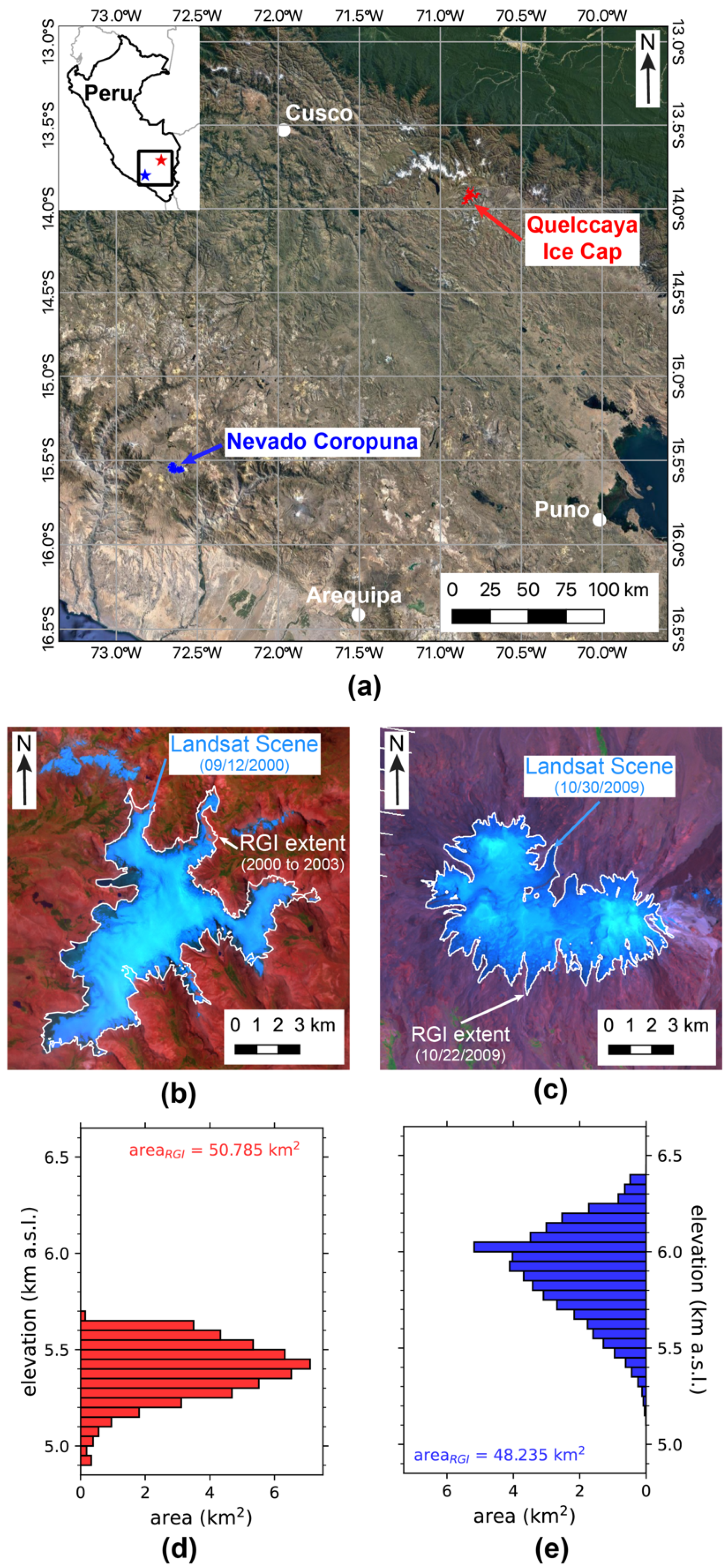
Study Sites

Glaciers in southern Peru are found on the eastern and western sides of the Andes Mountains. Over 88% of the glaciated area in Southern Peru is on the eastern side [11] and includes the Quelccaya Ice Cap (13.93° S, 70.82° W). The ice cap sits atop a broad plateau with a summit elevation of 5670 m above sea level (a.s.l.) and has a typical ice margin elevation of 5300 m a.s.l. with a few valley glaciers extending to below 5000 m a.s.l. [27] (Figure 1d). Glaciers on the western side of the Andes are primarily found atop tall peaks such as Nevado Coropuna (15.55° S, 72.63° W). There are 23 glaciers and three ice domes on Nevado Coropuna spanning from 6414 m a.s.l. to 5550 m a.s.l (north side) and 5100 m a.s.l. (south side) [13] (Figure 1e). While these two ice masses are geographically proximal, they have distinct glacial geometries, which can affect how they respond to similar climate changes [28].

Glaciers in southern Peru experience a climate setting characteristic of the outer tropics, with minimal thermal seasonality but a distinct wet (austral summer) and dry season (austral winter) [1,6]. The dry seasons runs from May/June through August/September, and the wet season runs from roughly October through May [3]. The transition from the dry to the wet season can vary year to year, and delays in the start of the wet season can lead to very negative mass balances [3]. At the Quelccaya Ice Cap, 70 to 80% of annual precipitation falls during the wet season [29]. At four weather stations near Nevado Coropuna, 70 to 90% of annual precipitation falls between December and March [30]. The Andes Mountains of Southern Peru also experience an east–west precipitation gradient due to the prevailing winds and orientation of the Andes. Moisture advects from the Amazon basin to the east, creating a wetter eastern side of the Andes and leaving the western side in a rain shadow [31]. Ice cores from Quelccaya’s summit find an accumulation rate of about 1.18 m water equivalent (w.e.) a⁻¹ [29]. At Nevado Coropuna, an ice core from a 6080 m a.s.l. saddle glacier finds an accumulation rate of 0.39 m w.e. a⁻¹ [30], which is much less than the accumulation rate at Quelccaya. The climate setting for the two ice masses can be further subdivided into the wet southern outer tropics for Quelccaya and dry outer tropics for Coropuna [32]. These subdivisions can also affect how these ice masses respond to similar climate changes [33].

2. Materials and Methods

To identify snow and ice cover near the Quelccaya Ice Cap and Nevado Coropuna, we used Landsat scenes and well-established semi-automated classification methods. We analyzed scenes from the mid-1980s through 2021 to quantify how each ice cap is responding to recent climate changes. To limit the likelihood that we included ephemeral snow cover as part of the glacial extent, we calculated the glacial extent for multiple Landsat scenes for each year. We analyzed all usable scenes (i.e., those with minimal cloud cover over the glaciated region) from 1 April through 31 December, choosing the scene with the smallest glacial area as the most accurate representation of the glacial extent. More details about the data (Section 2.1) and semi-automated classification methods (Section 2.2) are found below.

2.1. Data Sets

To track glacial extents over time, we analyzed 529 Landsat Collection 2, Level 1 scenes (199 for the Quelccaya Ice Cap and 330 for Nevado Coropuna). We accessed the data from the EarthExplorer site (https://earthexplorer.usgs.gov/ (accessed on 1 March 2022)). For the Quelccaya Ice Cap, scenes spanned from 1984 through 2021, excluding 2012, for which there are no usable scenes. For Nevado Coropuna, scenes spanned from 1986 through 2021. We analyzed all cloud-free scenes from 1 April through 31 December for each year and also analyzed some scenes where clouds shrouded part of the glaciated region. For scenes with partial cloud cover, we used the cloud-free scene with the smallest glacial area for that year to fill in the obstructed surface.

We used multispectral images from Landsat 4 (1982 to 2001), Landsat 5 (1984 to 2013), Landsat 7 (1999 to present), Landsat 8 (2013 to present), and Landsat 9 (2021 to present). At Quelccaya, we only used Landsat 7 scenes predating when the Scan Line Corrector failed (31 May 2003). After it failed, data gaps covered a significant portion of the ice cap. At Coropuna, we continued analyzing Landsat 7 scenes after the instrument failed. The data gaps due to the failure of the Scan Line Corrector either did not intercept the glaciated area or only partially intercepted its western side. To fill any data gaps in Landsat 7 scenes at Nevado Coropuna, we used a scene from another Landsat mission operational that year (Landsat 5 from 2003 to 2011, Landsat 8 from 2013 to present, and Landsat 9 starting in 2021), choosing the scene with the smallest glacial area. From the Landsat scenes, we obtained an evolving 2-D picture of the extent of each tropical ice mass.

To gain insight into the third dimension (elevation), we used the Shuttle Radar Topography Mission (SRTM) digital elevation model (DEM). We accessed the Version 3, 30-m DEM from Open Topography (https://opentopography.org/, accessed on 1 March 2022). The data were collected in February 2000 by the Space Shuttle Endeavor, and the Version 3 product has eliminated voids in the DEM. The 30 m void-filled SRTM DEM has been used in past inventories of Peruvian [11] and Bolivian [34] glaciers, and the 90 m void-filled version has been used in past studies of the Quelccaya Ice Cap [17,23]. With the DEM, we calculated the area-elevation distribution (i.e., hypsometry) of the ice masses for each scene and identified at what elevations glacial loss was occurring. We also used the DEM as part of the semi-automated land-surface classification algorithm (Section 2.2).

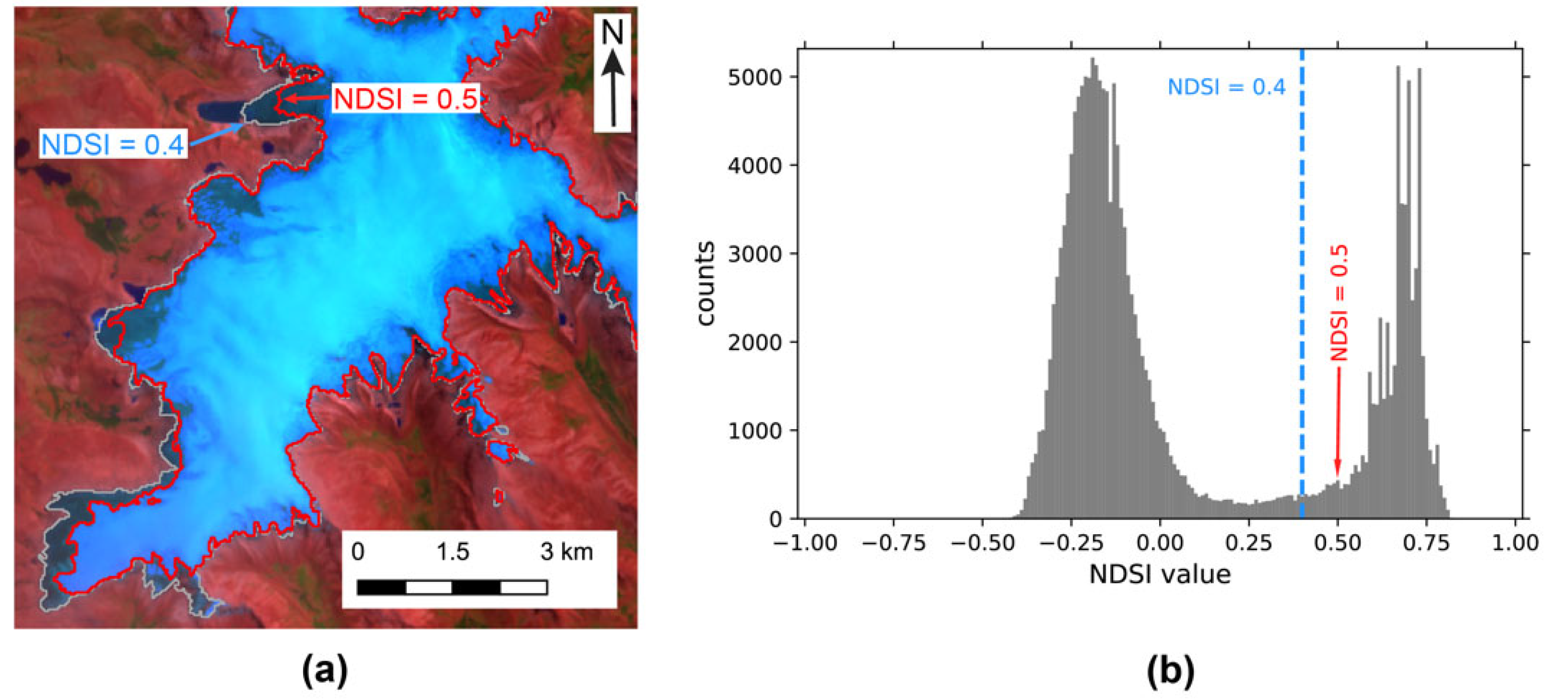
2.2. Semi-Automated Method to Determine Glacial Extents

Snow and ice have unique optical properties that enable us to differentiate them from other surface materials using multispectral data such as Landsat scenes. Commonly used approaches utilize the Normalized Difference Snow Index (NDSI) or a Band Ratio (BR) [13,17,22]. We combined both the NDSI and BR, which is a method that has been implemented to inventory glaciers in Peru [11] and Bolivia [34]. We calculated the NDSI using top-of-atmospheric reflectance of the green band and shortwave infrared 1 (SWIR1) band: NDSI = (Green − SWIR1)/(Green + SWIR1). For the BR, we used the digital number of the red band and SWIR1 band: BR = Red/SWIR1. We used the NDSI with a threshold of 0.5 to differentiate snow and ice (high NDSI values) from other surface materials (lower NDSI values). For pixels in deep shadows, we also used the BR with a threshold of 1.75 to identify snow and ice (high BR values).

The NDSI threshold value we used is lower than that used in other studies of outer tropical glaciers [11,13,34]. However, we found an NDSI threshold of 0.5 more consistently separates the high values attributed to snow and ice from the lower values attributed to other surface materials. We visually inspected the histogram of NDSI values for each scene to ensure that the threshold value of 0.5 accurately separated the bimodal distribution. For seven scenes at Quelccaya (3.5% of the total) and four scenes at Coropuna (1.3% of the total), we lowered the NDSI threshold to 0.4 to better separate the distribution since the higher threshold of 0.5 failed to include some of the ice near the edges as part of the glacial extent (Appendix A). Our BR threshold value aligns with previous studies [11,34], and we also visually inspected its histograms to ensure the validity of the threshold. We visually inspected all resulting masks, overlaying them on the corresponding false-color composite of the Landsat scene to ensure that it included the snow/ice in that scene.

After the NDSI and BR threshold algorithm, we converted the resulting black-and-white rasters of potentially glaciated pixels to polygons for manual post-processing. We filled small voids in the polygons (<6000 m²), which can be artifacts of the specific thresholds chosen. Additionally, we removed small polygons (<10,000 m²; 0.01 km²), assuming they were snowfields or ephemeral snow cover instead of glaciated areas. To determine which of the remaining polygons were part of the ice cap, we overlaid them on an earlier, lower spatial and spectral resolution Landsat scene (1975 for Quelccaya and 1980 for Coropuna). We removed any polygons that did not at least partially intercept the earlier extent, assuming these disparate polygons were snow patches instead of part of the former ice cap’s extent. Finally, for Quelccaya, we also implemented an algorithm to remove proglacial lakes, which have emerged as the ice cap has retreated [17].

Lakes can be falsely classified as being snow or ice by the NDSI or BR threshold classification algorithms since both liquid and solid water are more reflective at visible wavelengths (e.g., Green/Red) while much less reflective in at shortwave infrared (e.g., SWIR1) wavelengths. However, the Normalized Difference Water Index (NDWI) can identify pixels that are lakes even when they abut glaciers [17]. We calculated the NDWI using the top-of-atmospheric reflectance of the red band and near-infrared (NIR) band: NDWI = (Red − NIR)/(Red + NIR). Liquid water has a higher NDWI value, and we used a threshold value of between 0.1 and 0.2 to differentiate lakes from snow and ice. High NDWI values can also occur in shadowed regions [35]. To ensure we did not remove glaciated areas in shadows, we used the SRTM DEM to calculate the surface slope and only included as lakes those pixels with a slope less than 15°. We created one lake mask for each year and used it to remove proglacial lakes from each scene at Quelccaya. At Nevado Coropuna, which has a much drier climate, proglacial lakes have not emerged, and we did not include this step.

The semi-automated algorithm yielded polygons representing an estimate of the glacial extent for each Landsat scene analyzed. To quantify the uncertainty in each scene’s glacial extent, we used the Hanshaw & Bookhagen (2014) [17] method, which assumes uncertainty emerges due to misclassification of pixels along the perimeter of glaciated areas. The uncertainty of each polygon depends on the length of the perimeter (p) and the size of the pixel (G). We calculate the standard deviation of the uncertainty as follows: 1 − σ = (p/G) * ½ * 0.6872 * G². The uncertainty in each polygon is assumed to be independent, making the total uncertainty of the ice mass (σ_T) the following: σ_T = (σ₁² + σ₂² + … + σ_n²)^½. For each year, we chose the scene with the smallest glaciated area as the best representation of that year’s ice mass, which is an approach that has been used previously for tropical glaciers [13,17]. To calculate long-term trends, we perform ordinary least squares regressions on the annual time series of glacial areas, using the statsmodel module in Python.

3. Results

Figure 2 and Figure 3 present the changes at the Quelccaya Ice Cap and the glaciers on Nevado Coropuna, respectively. When tracking changes over time, we use 1988 as the starting year and 2020 as the ending year. 1988 was the first year where there were multiple scenes that we could analyze for both ice masses. 2020 was the most recent year at both ice masses that followed the observed long-term trend. La Niña conditions were observed in 2021, which tend to be wetter and colder, meaning the ice masses would be more likely to have ephemeral snow along their periphery. At the Quelccaya Ice Cap, the 2021 scene with the minimum area classified as glacial extent was anomalously large, suggesting that ephemeral snow cover had been included in the classification of that year’s extent (Figure 2c). At Nevado Coropuna, the 2021 scene with the minimum area classified as snow and ice is slightly larger than the 2020 minimum area scene (Figure 3c), making 2021 a poor candidate for the ending reference year. Thus, 2020 makes for a better ending year to characterize the long-term changes at each ice mass.

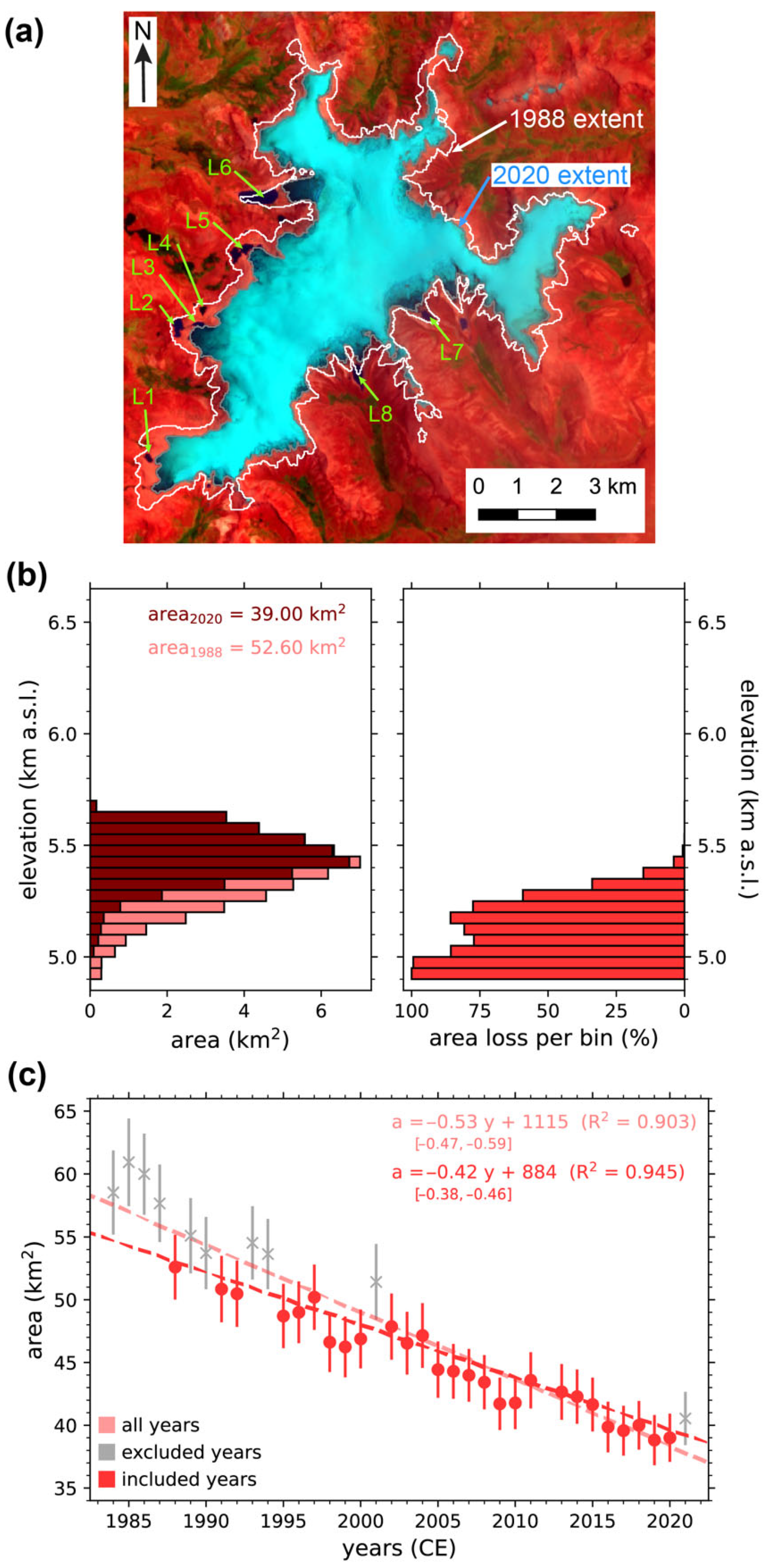
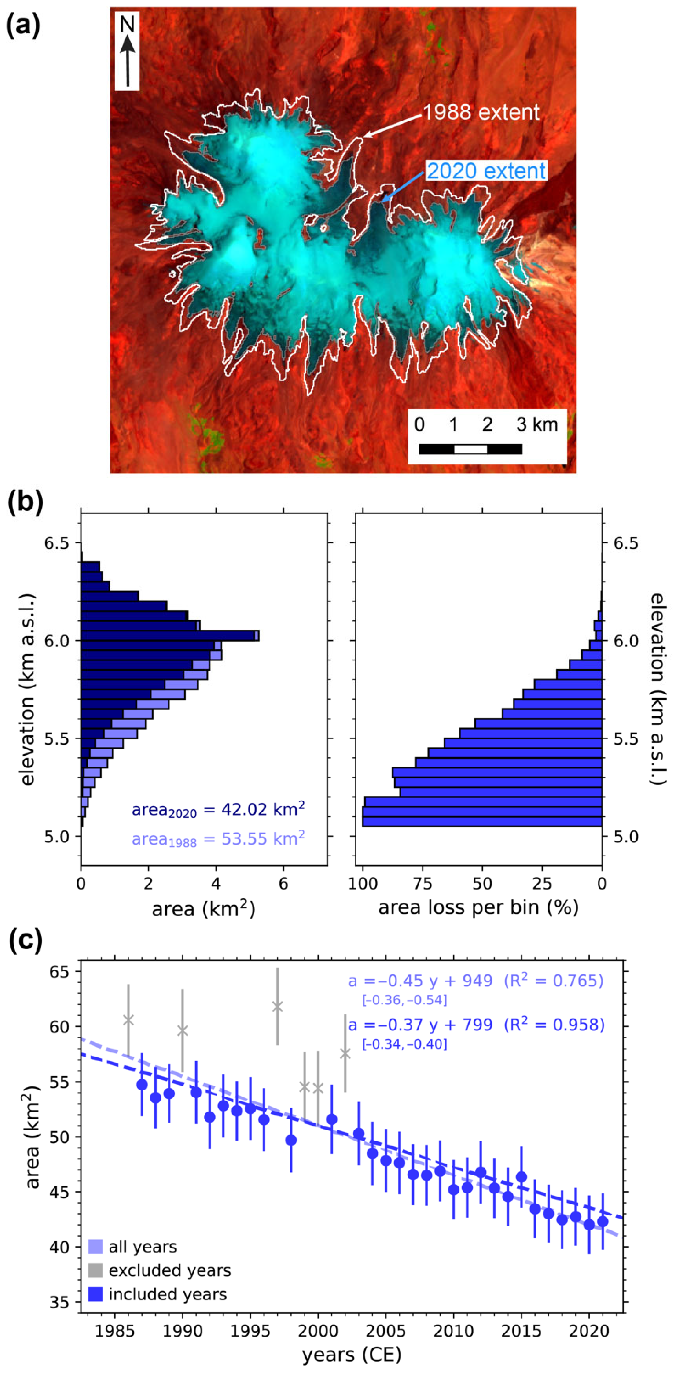
3.1. Evolution of the Quelccaya Ice Cap

The Quelccaya Ice Cap has retreated markedly since the mid-1980s (Figure 2). From 1988 to 2020, the ice cap shrunk by almost 26%: 52.60 ± 2.58 km² (+/−2-σ uncertainty) in 1988 to 39.00 +/− 1.92 km² in 2020. More loss has occurred on the western side of the ice cap than on the eastern side (Figure 2a). As the ice cap has shrunk, proglacial lakes have grown, and multiple lakes have emerged within the 1988 extent (Figure 2a). Most loss has occurred at lower elevations. Nearly all (>99%) of the ice cap in 1988 that was below 5000 m a.s.l. had been lost by 2020, and much (almost 85%) of it below 5200 m a.s.l. had disappeared (Figure 2b). As the ice cap has lost area at lower elevations, its mean elevation has risen from 5389 m a.s.l. to 5449 m a.s.l. (median from 5405 m a.s.l. to 5433 m a.s.l.). Additionally, it occupies a smaller range of elevations, with its interquartile range decreasing by 60 m. The Quelccaya Ice Cap of 2020 is a smaller, higher, and more restricted version of its 1988 self.

The ice loss has been relatively constant over the observation period (Figure 2c). From 1988 to 2020, 13.60 +/− 3.22 km² of ice cap area was lost, which translates to an average loss rate of 0.43 +/− 0.10 km² a⁻¹. This loss rate is indistinguishable from the loss rate by an ordinary least-squares linear regression of the glacial areas (0.42 km² a⁻¹), excluding outliers (Figure 2c). A linear model for ice cap evolution (i.e., constant loss rate) fits the data better than a quadratic (i.e., accelerating loss rate) or cubic (i.e., multiple changes in loss rate) model, according to an Akaike information criterion (AIC) analysis. A constant rate of area loss per year means that the percent loss per year is accelerating. A loss rate of 0.42 km² a⁻¹ translates to 0.8% a⁻¹ relative to the 1988 extent. The loss rate increased to over 0.9% a⁻¹ relative to the early/mid-2000 extents. For the 2020 extent, the loss rate is over 1% a⁻¹. Thus, the Quelccaya Ice Cap is losing glacial area at a constant rate and accelerating in its degree of change, depending on which metric is used to characterize its loss.

Including all the years in our regression analysis also yields a linear area loss rate, but its value is amplified by more than 27% (Figure 2c). We excluded ten years from our linear regression analysis (1984, 1985, 1986, 1987, 1989, 1990, 1993, 1994, 2001, 2021) since we inferred those years did not accurately represent the ice cap’s extent. These years have anomalously large areas, and we found through visual inspection that the extra area is likely due to ephemeral snow (see Appendix B). Many of the excluded years have only a few scenes we could analyze and did not include scenes spanning both the nominal dry season (May/June through August/September) and the extended period (October through December). Thus, our efforts to minimize the influences of ephemeral snow cover were less effective for many of the excluded years. For example, the 1984 ice cap area is >4.5 km² (>8%) larger than our regression model (excluding outliers) would predict, but there was only one June scene and one July scene we could analyze for that year. By excluding anomalous years from our analysis, we find that the Quelccaya Ice Cap is retreating but at a slightly reduced rate.

3.2. Evolution of the Glaciers on Nevado Coropuna

The glaciers on Nevado Coropuna have also retreated since the mid-1980s (Figure 3). From 1988 to 2020, the total glaciated area shrunk by over 21%: 53.55 +/− 2.80 km² (+/−2-σ uncertainty) in 1988 to 42.02 +/− 2.66 km² in 2020. The loss has occurred on all sides of the mountain as most of the valley glaciers have retreated upslope (Figure 3a). Most of the glacial area (>77%) in 1988 below 5500 m a.s.l. had disappeared by 2020, and virtually all of it (>99%) below 5200 m was gone (Figure 3b). However, a majority (>66%) of the total ice loss from 1988 to 2020 occurred between 5500 and 6000 m a.s.l. since only a small amount (<10%) of the glaciated area in 1988 was below 5500 m a.s.l. (Figure 3b). As the glaciers on Coropuna have retreated upslope, the mean elevation has risen from 5868 a.s.l. to 5940 m a.s.l. (median from 5896 m a.s.l. to 5961 m a.s.l.). The range of elevations has also contracted, with the interquartile range decreasing by 63 m. The glaciers on Nevado Coropuna in 2020—like the Quelccaya Ice Cap—are a smaller, higher, and more restricted version of their 1988 selves.

The loss of glacial area on Nevado Coropuna has also been relatively constant (Figure 3c). From 1988 to 2020, 11.53 +/− 3.86 km² of glacial area was lost, which translates to an average loss rate of 0.36 +/− 0.12 km² a⁻¹. This loss rate is indistinguishable from the loss rate by an ordinary least-squares linear regression over the interval (0.37 km² a⁻¹), excluding outliers (Figure 3c). A linear model (i.e., constant retreat loss rate) better fits the data than a quadratic (i.e., accelerating loss rate) or cubic (i.e., multiple changes in loss rate) model, according to an AIC analysis. Like the Quelccaya Ice Cap, the percent loss per year is accelerating. Relative to the 1988 extent, the loss rate was 0.67% a⁻¹. By the early/mid-2000s, it grew to 0.75% a⁻¹. It is about 0.85% a⁻¹ relative to the 2020 glacial area. The total glacial area at Nevado Coropuna—like at Quelccaya—is losing area at a constant rate and accelerating in its degree of change.

The rate of glacial area loss is also constant if all years are included in the analysis, but its value would be amplified by about 20% (Figure 2c). We excluded six years from our linear regression analysis (1986, 1990, 1997, 1999, 2000, 2002) since we inferred those years did not accurately represent the ice cap’s extent. The glacial areas for these years are anomalously large, and we found through visual inspection that the extra area is likely due to ephemeral snow (see Appendix B). As with Quelccaya, these years often had limited scenes we could analyze. In 1990, for example, there were no usable scenes after August. Thus, we could expect an anomalously large area for 1990 since Kochtitzky et al. (2018) [13] have demonstrated that the best scenes for analyzing glacial coverage at Nevado Coropuna are from November or December. The remaining excluded years had only one or two usable scenes from November and December. As we show in Section 4.1, the estimated glacial area for Nevado Coropuna is especially sensitive to which scene is used. Thus, by excluding anomalous years, we find that the glacial loss at Nevado Coropuna is more muted, but the loss is still pronounced and alarming.

4. Discussion

4.1. The Role of Scence Selection on Estimates of Glacial Extent

For remote sensing techniques to meaningfully expand our knowledge about glaciers, our techniques must accurately capture glacial extents. A potentially large source of inaccuracy can be introduced by analyzing scenes with ephemeral snow cover. An approach that has been used for outer tropical glaciers to reduce the influence of ephemeral snow cover is to analyze multiple scenes during the nominal dry season (May/June through August/September) and choose the one with the minimum area as the best representation of the glacial extent. However, Kochtitzky et al. (2018) [13] demonstrate that this method would overestimate the glacial extent at Nevado Coropuna (i.e., a dry outer tropical glacier), where the minimum typically occurs in November or December. Similar explicit analyses of scene selection have not been undertaken at the Quelccaya Ice Cap or other wet outer tropical glaciers. To undertake such an analysis, we used a subset of scenes from our study (374 scenes, 166 for Quelccaya, 208 for Coropuna). We select only scenes without visible snow in the surrounding landscape, a common pre-screening technique [13,17,19]. Polygons of the glacial extents for this subset are available in the online Supplemental Materials.

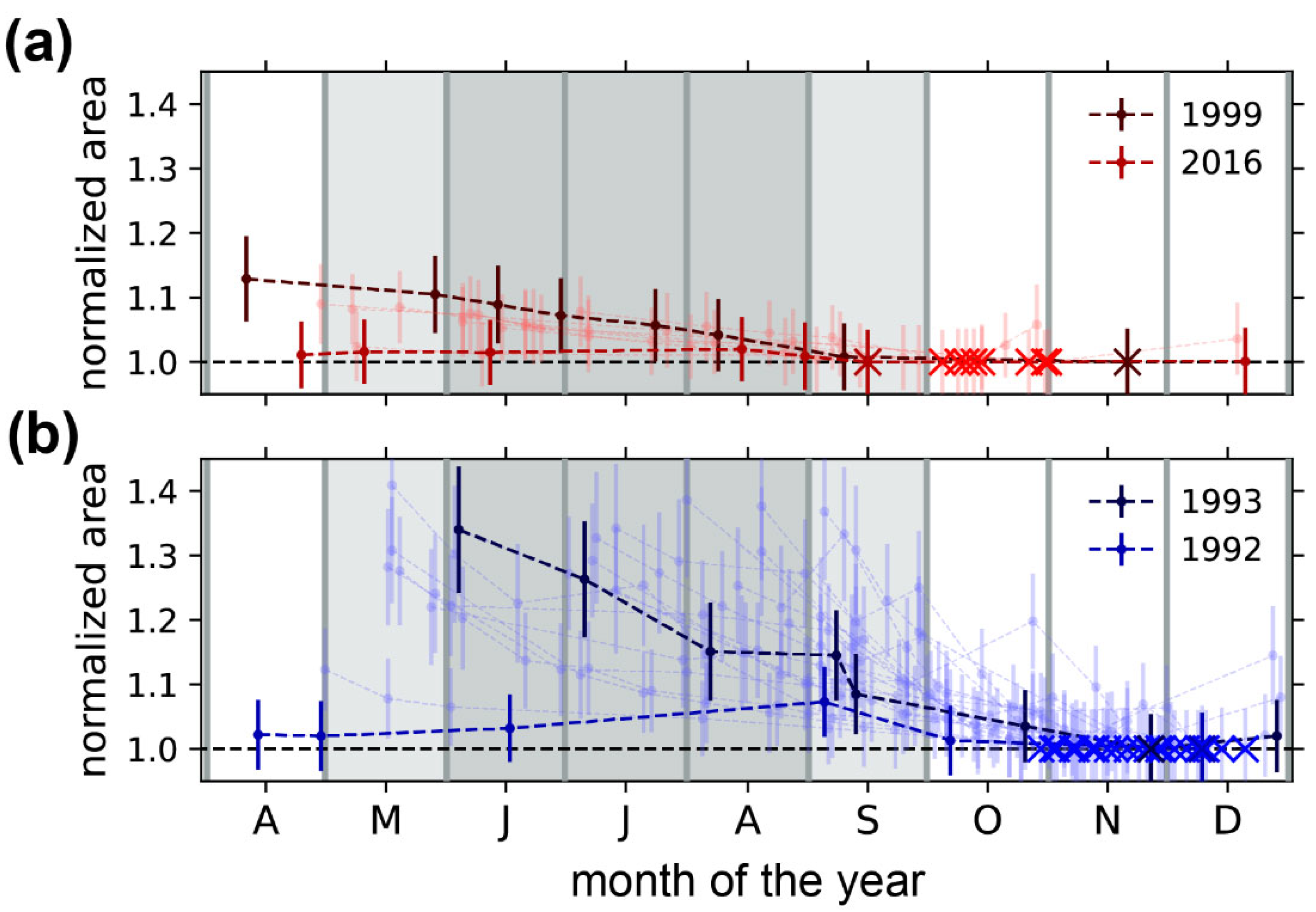
4.1.1. Optimal Time of Year for Scene Selection

At both the Quelccaya Ice Cap and Nevado Coropuna, we find that the optimal scene is from after the nominal dry season (see Tables S1 and S2 in the Supplemental Materials). At Quelccaya, the scene with the minimum area occurs in October or later for over 40% of the years (15 of 37). Over 24% of the years (9 of 37) have minimum areas for scenes in September, but most of these years (8 of 9; 89%) do not contain usable scenes from after September. All years with minimum areas for scenes before September (13 of 37; 35%) do not contain scenes from September or after. For years lacking useable scenes from after the nominal dry season, the estimated area may not represent the true ice cap extent since there could be ephemeral snow cover. Coincidentally, all the excluded years from Quelccaya’s regression analysis were ones that did not contain scenes from after the nominal dry season.

At Nevado Coropuna, the optimal scene tends to occur even later in the year. For almost 89% of the years (32 of 36), the minimum area occurs for a scene from November or December. About 8% of the years (3 of 36) have a minimum area for an October scene, but 2 of those years (1991 and 1995) do not contain scenes from after October. Only one year had a minimum area for a scene from before October, which was 1990. The latest useable scene for 1990 was from August. Thus, using scenes from the nominal dry season at the Quelccaya Ice Cap and Nevado Coropuna would likely yield larger estimates of the glacial areas than the true extent.

Previous remote sensing studies of the Quelccaya Ice Cap and Nevado Coropuna have preferentially analyzed scenes from the nominal dry season. At Nevado Coropuna, Kochtitzky et al. (2018) [13] illustrate that previous studies found divergent and elevated glacial retreat rates since they primarily analyzed scenes from the dry period. A subsequent regional inventory of glaciers in Southwestern Peru, which includes Nevado Coropuna, also used scenes mainly from the nominal dry season [11]. At the Quelccaya Ice Cap, Salzmann et al. (2013) [23] analyzed scenes exclusively from May through August, and Hanshaw & Bookhagen (2014) [17] analyzed scenes mainly from the dry season. Two recent regional inventories of glaciers in Southeastern Peru, which includes the Quelccaya Ice Cap, used scenes exclusively from the nominal dry season [11,18]. Remote sensing studies in other regions of the outer tropics have also mainly analyzed scenes from the nominal dry season, such as in the Cordillera Blanca, Peru [11,15,16,36] and eastern cordilleras of Bolivia [34,37,38]. These past studies have likely yielded artificially large glacier areas due to the choices of scenes analyzed. However, the impact of selecting a scene other than the annual minimum needs to be assessed.

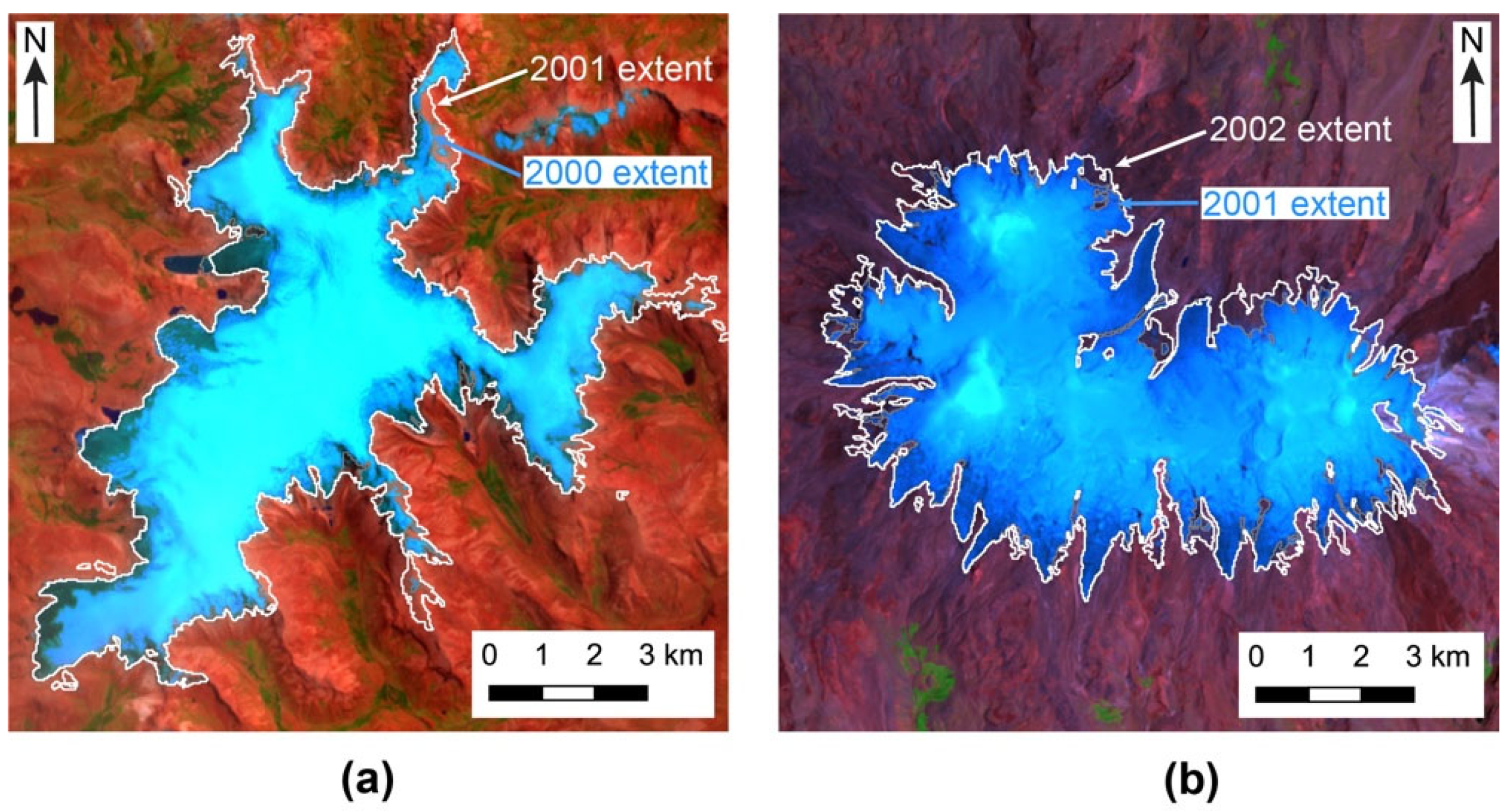
4.1.2. Impact of Selecting the Wrong Scene

To quantify the impact of scene selection on the estimates of glacial area, we compared the area of each scene in the subset to the minimum area of that year for all years that contained at least two scenes from the nominal dry season and two scenes from after the dry season (Figure 4). Nevado Coropuna has significantly more years that fulfill these criteria (22 years for Coropuna vs. 10 years for Quelccaya). One limit on the number of years for the Quelccaya Ice Cap was cloud cover, which was common over after the nominal dry season. Eighteen years were excluded from Figure 4a because these years lacked two scenes in the subset from after the nominal dry season—even though these years had enough scenes from the nominal dry season. At Nevado Coropuna, cloud cover was rare during and after the dry season. However, snow cover in the surrounding landscape was common at Nevado Coropuna during the nominal dry season. Eight years were excluded from Figure 4b because these years lacked two scenes in the subset from the nominal dry season—even though these years had enough scenes from after the nominal dry season.

For both tropical ice masses and most years, the timing of scene selection can affect the ability to accurately assess the ice cap margin, leading to inaccurate area estimates (Figure 4). This effect is greater at Nevado Coropuna where the area of snow and ice in scenes from the nominal dry season is, on average, 17% larger in area than the best estimate of the glacial area for that year. At the Quelccaya Ice Cap, the area of snow and ice in dry-season scenes is, on average, 4.3% larger but can be more than 10% larger. The 2-σ uncertainties in glacial areas are typically between 5 and 7%. Glaciated areas found from dry season scenes may not be significantly larger than the annual minimum for some years, but for most years, they tend to yield areas that are notably larger than the best estimate of the area (see highlighted curves in Figure 4). However, selecting any dry-season scenes does not ensure an accurate estimate of the glacial area. At Nevado Coropuna, scenes from October, November, and December that are not the annual minimum are, on average, 4.5% larger than the best estimate of the glacial area, and they can be as much as 19% larger. At the Quelccaya Ice Cap, scenes from after the dry season that are not the annual minimum are, on average, 2.6% larger, and they can be as much as 5.8% larger. To ensure accurate estimates of the glacial area—especially for Nevado Coropuna—multiple scenes should be analyzed from October, November, and December (i.e., after the nominal dry season).

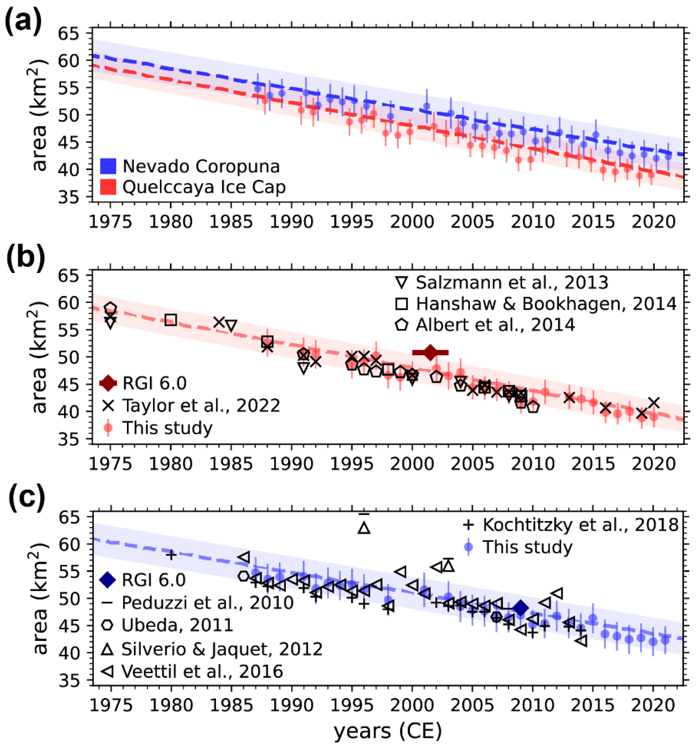
4.2. Updated Insights on the World’s Largest Tropical Ice Masses

We find that Nevado Coropuna has likely been the largest tropical ice mass since at least the 1980s. Over the entire observation window, the best estimate of the glacial area for Nevado Coropuna has been larger than the best estimate for the Quelccaya Ice Cap (Figure 5a). Additionally, the differences in best estimates have become more pronounced over time. In 1988, the glacial area at Nevado Coropuna was 53.55 +/− 2.80 km² (best estimate +/− 2-σ uncertainty), while the area of the Quelccaya Ice Cap was 52.60 +/− 2.58 km². In 2020, the glacial areas were 42.02 +/− 2.66 km² and 39.00 +/− 1.92 km², respectively. While the best estimates of the glacial area suggest that the Quelccaya Ice Cap is the smaller ice mass, the 2-σ uncertainties in the glacial area overlap for the entire observation window. However, the differences in size should become more pronounced in the future since the Quelccaya Ice Cap is shrinking more rapidly.

4.2.1. Extent and Evolution of the Quelccaya Ice Cap

Our best estimates for the Quelccaya Ice Cap yield a notably smaller ice cap than its size in the Randolph Glacier Inventory (RGI), but they are similar to some previous studies (Figure 5b). The RGI estimates an ice cap area of 50.79 km² for the interval between 2000 and 31 May 2003. For 2000, we find the ice cap is 46.88 +/− 2.34 km²; for 2002, it is 47.86 +/− 2.64 km², and for 2003 it is 46.54 km +/− 2.50 km². We did not include the 2001 extent in our linear regression analysis because its area estimate (51.32 +/− 3.02 km²) is anomalously large, and there were no scenes that year from after the nominal dry season that we could analyze. If the RGI’s value were used for a current estimate, then it would yield an area 30% larger than the 2020 extent. Previous studies on the evolution of the Quelccaya Ice Cap [17,18,23,39] largely overlap with the 2-σ uncertainties of our findings (Figure 5b). While our values for Quelccaya’s area tend to overlap with previous studies, our trend for how the ice cap is changing differs from those reported previously.

We find that the Quelccaya Ice Cap is shrinking linearly at a rate of −0.42 [−0.38, −0.46] km² a⁻¹, where the values in square brackets are the 95% confidence interval. Hanshaw & Bookhagen (2014) [17] and Albert et al. (2014) [39] also find the Quelccaya Ice Cap is shrinking linearly, but they find larger loss rates. Albert et al. (2014) [39] find a rate of −0.52 km² a⁻¹. Using the Hanshaw & Bookhagen (2014) [17] values for the main ice cap, we calculate a rate of −0.47 [−0.44, −0.50] km² a⁻¹. Their elevated loss rates compared to ours may reflect the time interval of their analysis. In both studies, the last year in their dataset is from the 2009/2010 El Niño event, when ephemeral snow cover should be minimal. We find that Quelccaya’s area in 2009 and 2010 are smaller-than-would-be-expected by the long-term trend (Figure 2c). Ending their analyses with a notably small year could amplify their loss rates. Both studies included data from before our earliest year in the analysis (1988), but their earlier values still fall within our long-term linear trend (Figure 5b). By utilizing data from the most recent decade, our findings provide an updated estimate of the loss rate of the Quelccaya Ice Cap.

A linear evolution of the ice cap, at first, appears to conflict with the findings of Salzmann et al. (2013) [23] and Taylor et al. (2022) [21], which suggest that the ice cap has shrunk at different rates at different times. Both studies find a smaller loss rate before the mid-1980s, but this finding may be an artifact of the dearth of scenes before the mid-1980s. Loss rates before the mid-1980s are based on two (three) scenes spanning a decade (more than two decades), making them susceptible to noise in the data. Additionally, the data from [21] suggest that the loss rate has recently weakened, but this finding may be an artifact of their area estimate for 2020. Their estimate of the area in 2020 is notably larger than their estimate for the area in 2019, which would weaken the current loss rate. While we also find that Quelccaya’s area in 2020 is slightly larger than its 2019 area, our 2020 value is consistent with a linear evolution of the ice cap (Figure 2c). However, the data from these past studies might also be consistent with our findings since their area estimates intercept the predictions of our linear model for the ice cap’s evolution (Figure 5b). In summary, we find that the Quelccaya Ice Cap has been shrinking at a constant rate, and a linear model for its evolution can predict many of the previously published estimates of its size.

4.2.2. Extent and Evolution of the Glaciers on Nevado Coropuna

Our best estimates for the glacial coverage on Nevado Coropuna yield glacial areas similar to those found in past studies that analyzed scenes from after the nominal dry season (Figure 5c). In the RGI, glaciers on Nevado Coropuna cover an area of 48.24 km² based on a 22 October 2009 scene. We find a glacial area on Coropuna in 2009 of 46.89 +/− 2.78 km² (for a 30 October 2009 scene). However, if the RGI’s value were used for a current estimate, then it would yield an area about 15% larger than the 2020 extent. Our area estimates are also similar to two studies that analyzed scenes from after the dry season. Area estimates from Kochtitzky et al. (2018) [13] are similar to ours—albeit slightly smaller (Figure 5c). Our estimates are, on average, 1.17 km² (2.56%) larger, but this difference is within 2-σ uncertainties. Our larger estimates of the glacial area may reflect our lower NDSI threshold (0.5 for this study vs. 0.5567 for theirs) and how the glacial coverage on Coropuna was defined (all polygons that fall at last partially within the 1980 extent for this study vs. the largest single polygon in theirs). The area estimates from Úbeda (2011) [40] are also similar to ours; their estimate for the 2007 glacial area differs from ours by less than 0.02 km² (Figure 5c). Utilizing dry season scenes, however, does not ensure an accurate representation of the glacial extent. Racoviteanu et al. (2007) [41] estimate a 2000 glacial extent of 60.8 km² using a 14 October ASTER image, whereas our 2000 estimate is 54.4 +/− 3.38 km² using a 14 November Landsat scene. To accurately represent Coropuna’s glacial area, we must select scenes from after the nominal dry season and analyze multiple scenes from this interval.

Studies that primarily used scenes from the nominal dry season vastly overestimate the glacial extent of Nevado Coropuna. Peduzzi et al. (2010) [24] find substantially larger glacial areas for 1996 and 2003, using scenes from June and May, respectively (Figure 5c). Their 1980 estimate (>80 km²) could not be displayed within our y-axis range in Figure 5c. Their 2008 area estimate, which is from a late-September scene, is closer to our estimate, which is from a mid-November scene. Silverio & Jaquet (2012) [25], who analyzed scenes from late July through early September, also found glacial areas significantly larger than ours (Figure 5c). Only their 1996 and 2003 areas could be displayed within the y-axis range of Figure 5c. Their 1985 estimate (96 km²) and 1975 estimate (105 km²) greatly exceeded what our data would suggest. Veettil et al. (2016) [26] also primarily analyzed dry-season scenes, and their estimates are more variable year-to-year than ours and often much larger (Figure 5c). Overestimates of Coropuna’s glacial extent are common in studies that used scenes from the dry season, which can affect assessments of its glaciers as a water resource and understanding of how they change with time [13].

We find that Coropuna’s glacial area has been shrinking linearly at a rate of −0.37 [−0.34, −0.40] km² a⁻¹. Kochtitzky et al. (2018) [13] also find that the ice cap is shrinking linearly, and they report a rate of −0.409 km² a⁻¹ by differing their 1980 and 2014 glacial areas. Performing a least-squares linear regression on their data yields a rate of −0.35 [−0.30, −0.41] km² a⁻¹, which agrees well with our findings. Previous studies that mainly analyzed scenes from the dry season also report linear loss rates, but they are sustainably larger. Silverio & Jaquet (2012) [25] report a loss rate of 1.4 km² a⁻¹, and the Peduzzi et al. (2010) [24] data since 1980 yield a loss rate of about 1.1 km² a⁻¹ by least-squares linear regression. High loss rates from many previous studies likely reflect ephemeral snow cover and, as discussed in [13], lead to inaccurate projections for how long the glaciers on Nevado Coropuna will remain a viable water resource.

On top of the long-term linear retreat of Coropuna’s glaciers, we find year-on-year fluctuations in glacial area, which we attribute to noise due to ephemeral snow cover. Veettil et al. (2016) [26] also note year-on-year fluctuations but interpret many of them as periods of accelerated retreat of readvance. Many of these fluctuations occur during El Nino and La Nina events. While El Niño (La Niña) events tend to produce negative (neutral to slightly positive) mass balances for outer tropical glaciers [2,3], it is unlikely that these year-on-year fluctuations reflect changes in the glacial evolution. It takes time for mass balance anomalies to propagate to the terminus, and even with a fast response time, changes in terminus positions can lag by multiple years [42]. Additionally, the year-on-year fluctuations in Veettil et al. (2016) [26] (3 to 6 km²) would be unprecedented relative to the longer-term loss rate (<0.4 km² a⁻¹). Since the estimates of glacial extent for Nevado Coropuna are strongly impacted by scene selection (Section 4.1.2; Figure 4), ephemeral snow cover is a better explanation for these fluctuations. To isolate the evolution in Coropuna’s extent, we need multiple years of area estimates to separate the trend from noise due to epithermal snow cover.

A linear evolution of the glacial coverage on Nevado Coropuna conflicts with some previous studies. Silverio & Jaquet (2012) [25] find a lower loss rate before 1985, an increased loss between 1985 and 1996, and a slightly reduced loss rate after 1996. Peduzzi et al. (2010) [24] find that models with negative and positive curvature can capture the trends in glacial coverage between 1955 and 2008. However, these findings may be artifacts of low temporal resolution. Silverio & Jaquet (2012) [25] draw their trends from data spaced half a decade to multiple decades apart, and Peduzzi et al. (2010) [24] build their models from five measurements between 1955 and 2008. Additionally, both studies may be impacted by ephemeral snow cover since they used scenes primarily from the nominal dry season. Our data suggest that the glacial coverage on Nevado Coropuna has been shrinking linearly since 1988, and our linear model can predict the 1980 glacial coverage reported by Kochtitzky et al. (2018) [13] (Figure 5c). Estimates of Coropuna’s glacial extent before 1980 vary widely, and we cannot evaluate our linear model before then. Úbeda (2011) [40] found a 1955 glacial area that is smaller than the 1980 area from Kochtitzky et al. (2018) [13], implying that the glacial area grew before 1980. Silverio & Jaquet (2012) [25] found a glacier area in 1955 and Ames et al. (1988) [14] found a glacial area in 1962 that would require an amplified loss rate before 1980. To determine if the linear evolution of glacial coverage on Nevado Coropuna continued before 1980, future studies are needed using remote sensing data collected from after the nominal dry season.

5. Conclusions

We reassessed the evolution of the Quelccaya Ice Cap (Peru) and the glaciers on Nevado Coropuna (Peru) using Landsat scenes (i.e., remote sensing data) and methods to limit the influence of ephemeral snow cover. We find that Nevado Coropuna has been the largest tropical ice mass since at least 1988 and likely through the 1980s. In 1988, the glacial area on Nevado Coropuna was 53.55 +/− 2.80 km², and the glacial area of the Quelccaya Ice Cap was 52.60 +/− 2.58 km². By 2020, the glacial areas were 42.04 +/− 2.66 km² and 39.00 +/− 1.92 km², respectively. Both ice masses are shrinking at a constant rate (i.e., linear evolution): −0.42 [−0.38, −0.46] km² a⁻¹ for Quelccaya and −0.37 [−0.34, −0.40] km² a⁻¹ for Coropuna. Though the retreat rates overlap within their 95% confidence intervals, the difference in size between the two ice masses will likely become more pronounced in the future due to the larger central retreat rate at the Quelccaya Ice Cap (Figure 5a). Our estimates of the loss rates at both ice masses are smaller than those previously reported.

We also demonstrate that the optimal time of year to remotely track the two largest tropical ice masses is after the nominal dry season. By analyzing Landsat scenes from October, November, and December (i.e., after the nominal dry season), we can provide improved estimates of the glacial extents by minimizing the likelihood of including ephemeral snow cover in our glacier classification. Ephemeral snow cover is a larger issue for estimating the glacial extents at Nevado Coropuna, making scene selection vital for accurately monitoring its glaciers. We recommend that remote sensing studies of Nevado Coropuna—and other dry, outer tropical glaciers—analyze multiple scenes each year from October through December to characterize the glacial extents more accurately. We also recommend that remote sensing studies of the Quelccaya Ice Cap—and other wet, outer tropical glaciers—include scenes from after the nominal dry season. By reassessing the size and evolution of the two largest tropical ice masses using remote sensing data from after the nominal dry season, we provide new insights into their size and evolution.

As glaciers in the outer tropics continue to shrink and disappear in a warming world, communities in their shadows need continued monitoring of their size and changes. Most previous studies of outer tropical glaciers have analyzed data almost exclusively from the dry season, which might not accurately represent the glacial extent. We hope our findings and recommendations aid future studies on outer tropical glaciers to ensure accurate knowledge about their extents and evolution.

References

- Kaser, G.; Osmaston, H. Tropical Glaciers; Cambridge University Press: Cambridge, UK, 2002. [Google Scholar]
- Vuille, M.; Francou, B.; Wagnon, P.; Juen, I.; Kaser, G.; Mark, B.G.; Bradley, R.S. Climate change and tropical Andean glaciers: Past, present, and future. Earth Sci. Rev. 2008, 89, 79–96. [Google Scholar] [CrossRef]
- Rabatel, A.; Francou, B.; Soruco, A.; Gomez, J.; Cáceres, B.; Caballos, J.L.; Basantes, R.; Vuille, M.; Sicart, J.E.; Huggel, C.; et al. Current state of glaciers in the tropical Andes: A multi-century perspective on glacier evolution and climate change. Cryosphere 2013, 7, 81–102. [Google Scholar] [CrossRef]
- Vuille, M.; Carey, M.; Huggel, C.; Buytaert, W.; Rabatel, A.; Jacobsen, D.; Soruco, A.; Villacis, M.; Yarleque, C.; Timm, O.E.; et al. Rapid decline of snow and ice in the tropical Andes–Impacts, uncertainties and challenges ahead. Earth Sci. Rev. 2018, 176, 195–213. [Google Scholar] [CrossRef]
- Veettil, B.K.; Kamp, U. Global disappearance of Tropical Mountain Glaciers: Observations, Causes, and Challenges. Geosciences 2019, 9, 196. [Google Scholar] [CrossRef]
- Kaser, G. Glacier-climate interactions at low latitudes. J. Glaciol. 2001, 47, 195–204. [Google Scholar] [CrossRef]
- Mark, B.G.; Seltzer, G.O. Tropical glacier meltwater contribution to stream discharge: A case study in the Cordillera Blanca, Peru. J. Glaciol. 2003, 49, 271–281. [Google Scholar] [CrossRef]
- Soruco, A.; Vincent, C.; Rabatel, A.; Francou, B.; Thibert, E.; Sicart, J.E.; Condom, T. Contribution of glacier runoff to water resources of La Paz city, Bolivia (16° S). Ann. Glaciol. 2015, 56, 147–153. [Google Scholar] [CrossRef]
- Vergara, W.; Deeb, A.; Valencia, A.; Bradley, R.; Francou, B.; Zarzar, A.; Grünwaldt, A.; Haeussling, S. Economic impacts of rapid glacier retreat in the Andes. Eos Trans. Am. Geophys. Union 2007, 88, 261–264. [Google Scholar] [CrossRef]
- Kaser, G. A review of the modern fluctuations of tropical glaciers. Glob. Planet. Chang. 1999, 22, 93–103. [Google Scholar] [CrossRef]
- Seehaus, T.; Malz, P.; Sommer, C.; Lippi, S.; Cochachin, A.; Braun, M. Changes of the tropical glaciers throughout Peru between 2000 and 2016–mass balance and area fluctuations. Cryosphere 2019, 13, 2537–2556. [Google Scholar] [CrossRef] [Green Version]
- Thompson, L.G.; Mosley-Thompson, E.; Brecher, H.; Davis, M.; León, B.; Les, D.; Lin, P.N.; Mashiotta, T.; Mountain, K. Abrupt tropical climate change: Past and present. Proc. Natl. Acad. Sci. USA 2006, 103, 10536–10543. [Google Scholar] [CrossRef] [PubMed]
- Kochtitzky, W.H.; Edwards, B.R.; Enderlin, E.M.; Marino, J.; Marinque, N. Improved estimates of glacier change rates at Nevado Coropuna Ice Cap, Peru. J. Glaciol. 2018, 64, 175–184. [Google Scholar] [CrossRef]
- Ames, A.; Evangelista, P.; Valverde, A.; Zúñiga, J. Inventario de Glaciares del Perú; Consejo Nacional de Ciencia y Tecnologia: Huaraz, Peru, 1988; Part 1. [Google Scholar]
- Silverio, W.; Jaquet, J.M. Glacial cover mapping (1987–1996) of the Cordillera Blanca (Peru) using satellite imagery. Remote Sens. Environ. 2005, 95, 342–350. [Google Scholar] [CrossRef]
- Racoviteanu, A.E.; Arnaud, Y.; Williams, M.W.; Ordonez, J. Decadal changes in glacier parameters in the Cordillera Blanca, Peru, derived from remote sensing. J. Glaciol. 2008, 54, 499–510. [Google Scholar] [CrossRef]
- Hanshaw, M.N.; Bookhagen, B. Glacial areas, lake areas, and snow lines from 1975 to 2012: Status of the Cordillera Vilcanota, including the Quelccaya Ice Cap, northern central Andes, Peru. Cryosphere 2014, 8, 359–376. [Google Scholar] [CrossRef]
- Taylor, L.S.; Quincey, D.J.; Smith, M.W.; Potter, E.R.; Castro, J.; Fyffe, C.L. Multi-Decadal Glacier Area and Mass Balance Change in the Southern Peruvian Andes. Front. Earth Sci. 2022, 10, 863933. [Google Scholar] [CrossRef]
- Paul, F. Combined technologies allow rapid analysis of glacier changes. Eos Trans. Am. Geophys. Union 2002, 83, 253–261. [Google Scholar] [CrossRef]
- Paul, F.; Kääb, A.; Haeberli, W. Recent glacier changes in the Alps observed by satellite: Consequences for future monitoring strategies. Glob. Planet. Chang 2007, 56, 111–122. [Google Scholar] [CrossRef]
- Paul, F.; Frey, H.; Le Bris, R. A new glacier inventory for the European Alps from Landsat TM scenes of 2003: Challenges and results. Ann. Glaciol. 2011, 52, 144–152. [Google Scholar] [CrossRef]
- Albert, T.H. Evaluation of remote sensing techniques for ice-area classification applied to the tropical Quelccaya Ice Cap, Peru. Polar Geogr. 2002, 26, 210–226. [Google Scholar] [CrossRef]
- Salzmann, N.; Huggel, C.; Rohrer, M.; Silverio, W.; Mark, B.G.; Burns, P.; Portocarrero, C. Glacier changes and climate trends derived from multiple sources in the data scarce Cordillera Vilcanota region, southern Peruvian Andes. Cryosphere 2013, 7, 103–118. [Google Scholar] [CrossRef]
- Peduzzi, P.; Herold, C.; Silverio, W. Assessing high altitude glacier thickness, volume and area changes using field, GIS and remote sensing techniques: The case of Nevado Coropuna (Peru). Cryosphere 2010, 4, 313–323. [Google Scholar] [CrossRef]
- Silverio, W.; Jaquet, J.M. Multi-temporal and multi-source cartography of the glacial cover of Nevado Coropuna (Arequipa, Peru) between 1955 and 2003. Int. J. Remote Sens. 2012, 33, 5876–5888. [Google Scholar] [CrossRef]
- Veettil, B.K.; Bremer, U.F.; de Souza, S.F.; Maier, É.L.B.; Simões, J.C. Variations in annual snowline and area of an ice-covered stratovolcano in the Cordillera Ampato, Peru, using remote sensing data (1986–2014). Geocarto Int. 2016, 31, 544–556. [Google Scholar] [CrossRef]
- Yarleque, C.; Vuille, M.; Hardy, D.R.; Timm, O.E.; De la Cruz, J.; Ramos, H.; Rabatel, A. Projections of the future disappearance of the Quelccaya Ice Cap in the Central Andes. Sci. Rep. 2018, 8, 15564. [Google Scholar] [CrossRef]
- Oerlemans, J. Glaciers and Climate Change; A.A. Balkema Publishers: Lisse, The Netherlands, 2001. [Google Scholar]
- Thompson, L.G.; Mosley-Thompson, E.; Davis, M.E.; Zagorodnov, V.S.; Howat, I.M.; Mikhalenko, V.N.; Lin, P.N. Annually resolved ice core records of tropical climate variability over the past ~1800 years. Science 2013, 340, 945–950. [Google Scholar] [CrossRef]
- Herreros, J.; Moreno, I.; Taupin, J.D.; Ginot, P.; Patris, N.; De Angelis, M.; Ledru, M.P.; Delachaux, F.; Schotterer, U. Environmental records from temperate glacier ice on Nevado Coropuna saddle, southern Peru. Adv. Geosci. 2009, 22, 27–34. [Google Scholar] [CrossRef]
- Garreaud, R.D.; Vuille, M.; Compagnucci, R.; Marengo, J. Present-day South American climate. Palaeogeogr. Palaeoclimatol. Palaeoecol. 2009, 281, 180–195. [Google Scholar] [CrossRef]
- Sagredo, E.A.; Lowell, T.V. Climatology of Andean glaciers: A framework to understand glacier response to climate change. Glob. Planet. Chang. 2012, 86, 101–109. [Google Scholar] [CrossRef]
- Sagredo, E.A.; Rupper, S.; Lowell, T.V. Sensitivities of the equilibrium line altitude to temperature and precipitation changes along the Andes. Quat. Res. 2014, 81, 355–366. [Google Scholar] [CrossRef]
- Seehaus, T.; Malz, P.; Sommer, C.; Soruco, A.; Rabatel, A.; Braun, M. Mass balance and area changes of glaciers in the Cordillera Real and Tres Cruces, Bolivia, between 2000 and 2016. J. Glaciol. 2020, 66, 124–136. [Google Scholar] [CrossRef]
- Huggel, C.; Kääb, A.; Haeberli, W.; Teysseire, P.; Paul, F. Remote sensing based assessment of hazards from glacier lake outbursts: A case study in the Swiss Alps. Can. Geotech. J. 2002, 39, 316–330. [Google Scholar] [CrossRef]
- Burns, P.; Nolin, A. Using atmospherically-corrected Landsat imagery to measure glacier area change in the Cordillera Blanca, Peru from 1987 to 2010. Remote Sens. Environ. 2014, 140, 165–178. [Google Scholar] [CrossRef]
- Cook, S.J.; Kougkoulos, I.; Edwards, L.A.; Dortch, J.; Hoffmann, D. Glacier change and glacial lake outburst flood risk in the Bolivian Andes. Cryosphere 2016, 10, 2399–2413. [Google Scholar] [CrossRef]
- Veettil, B.K.; Wang, S.; Simões, J.C.; Pereira, S.F.R. Glacier monitoring in the eastern mountain ranges of Bolivia from 1975 to 2016 using Landsat and Sentinel-2 data. Environ. Earth Sci. 2018, 77, 452. [Google Scholar] [CrossRef]
- Albert, T.; Klein, A.; Kincaid, J.L.; Huggel, C.; Racoviteanu, A.E.; Arnaud, Y.; Silverio, W.; Ceballos, J.L. Remote sensing of rapidly diminishing tropical glaciers in the northern Andes. In Global Land Ice Measurements from Space; Kargel, J.S., Leonard, G.J., Bishop, M.P., Kääb, A., Raup, B.H., Eds.; Springer: Berlin/Heidelberg, Germany, 2014; pp. 609–638. [Google Scholar] [CrossRef]
- Úbeda, P.J. El Impacto del Cambio Climático en Los Glaciares del Complejo Volcánico Nevado Coropuna, (Cordillera Occidental de Los Andes Centrales). Ph.D. Thesis, Universidad Complutense de Madrid, Madrid, Spain, 2010. Available online: https://eprints.ucm.es/id/eprint/12076/ (accessed on 1 June 2022).
- Racoviteanu, A.E.; Manley, W.F.; Arnaud, Y.; Williams, M.W. Evaluating digital elevation models for glaciologic applications: An example from Nevado Coropuna, Peruvian Andes. Glob. Planet. Chang. 2007, 59, 110–125. [Google Scholar] [CrossRef]
- Roe, G.H.; Baker, M.B. Glacier response to climate perturbations: An accurate linear geometric model. J. Glaciol. 2014, 60, 670–684. [Google Scholar] [CrossRef] [Green Version]
Publisher’s Note: MDPI stays neutral with regard to jurisdictional claims in published maps and institutional affiliations. |
© 2022 by the authors. Licensee MDPI, Basel, Switzerland. This article is an open access article distributed under the terms and conditions of the Creative Commons Attribution (CC BY) license (https://creativecommons.org/licenses/by/4.0/).
Share and Cite
Malone, A.G.O.; Broglie, E.T.; Wrightsman, M. The Evolution of the Two Largest Tropical Ice Masses since the 1980s. Geosciences 2022, 12, 365. https://doi.org/10.3390/geosciences12100365
Malone AGO, Broglie ET, Wrightsman M. The Evolution of the Two Largest Tropical Ice Masses since the 1980s. Geosciences. 2022; 12(10):365. https://doi.org/10.3390/geosciences12100365
Chicago/Turabian StyleMalone, Andrew G. O., Eleanor T. Broglie, and Mary Wrightsman. 2022. "The Evolution of the Two Largest Tropical Ice Masses since the 1980s" Geosciences 12, no. 10: 365. https://doi.org/10.3390/geosciences12100365
APA StyleMalone, A. G. O., Broglie, E. T., & Wrightsman, M. (2022). The Evolution of the Two Largest Tropical Ice Masses since the 1980s. Geosciences, 12(10), 365. https://doi.org/10.3390/geosciences12100365