Article

Impact of Well Placement in the Fractured Geothermal Reservoirs Based on Available Discrete Fractured System

1
Group of Geothermal Science and Technology, Institute of Applied Geosciences, Technische Universität Darmstadt, 64287 Darmstadt, Germany
2
Darmstadt Graduate School of Excellence Energy Science and Engineering, Technische Universität Darmstadt, 64287 Darmstadt, Germany
*
Authors to whom correspondence should be addressed.
Geosciences 2022, 12(1), 19; https://doi.org/10.3390/geosciences12010019
Submission received: 23 September 2021 / Revised: 25 December 2021 / Accepted: 30 December 2021 / Published: 4 January 2022

Abstract

:
Well placement in a given geological setting for a fractured geothermal reservoir is necessary for enhanced geothermal operations. High computational cost associated with the framework of fully coupled thermo-hydraulic-mechanical (THM) processes in a fractured reservoir simulation makes the well positioning a missing point in developing a field-scale investigation. To enhance the knowledge of well placement for different working fluids, we present the importance of this topic by examining different injection-production well (doublet) positions in a given fracture network using coupled THM numerical simulations. Results of this study are examined through the thermal breakthrough time, mass flux, and the energy extraction potential to assess the impact of well position in a two-dimensional reservoir framework. Almost ten times the difference between the final amount of heat extraction is observed for different well positions but with the same well spacing and geological characteristics. Furthermore, the stress field is a strong function of well position that is important concerning the possibility of high-stress development. The objective of this work is to exemplify the importance of fracture connectivity and density near the wellbores, and from the simulated cases, it is sufficient to understand this for both the working fluids. Based on the result, the production well position search in the future will be reduced to the high-density fracture area, and it will make the optimization process according to the THM mechanism computationally efficient and economical.

1. Introduction

Geothermal field development and management is a complex process. Engineering a geothermal system requires appropriate well placement and fracture connectivity to ensure well connectivity and least fluid loss [1,2]. Placement of injection and production wells or a doublet system in a given geological framework to achieve maximum geothermal energy extraction is one of the most complicated and expensive procedures. The location of the injection well concerning production well decides the production mass flux [3,4]. Practically, there is an infinite number of sites where an injection well can be placed in designing an enhanced geothermal system (EGS). Well placement in association with fracture network requires two critical aspects to ensure high heat extraction potential. First, the fractures must be connected sufficiently, and they must provide a high fluid flow rate at a low-pressure difference, and secondly, fluid residence time in the fractures should be increased to allow sufficient heat exchange. Longer residence time enhances the heat extraction capacity and reduces the chances of short-circuiting [5,6]. Figure 1 shows a subsurface fracture network where red is the high-temperature region. Hot water is produced through the red color well from the reservoir, and after passing it through the heat exchanger, it is reinjected to the reservoir with the blue color well. Fractures are the main paths for fluid flow that allow for heat extraction from the various MEET geothermal sites, including Soultz sous Forêts, United Down, Göttingen, and Havelange. Discrete Fracture Network (DFN) characterization is an essential step toward the simulation of reservoir performance. However, the total number of fractures resulting from DFN characterization is a high number (in the order of millions of fractures) which is not feasible for performing numerical simulation (due to computational costs) while considering all of them discretely through the thermal-hydraulic (TH) or thermal-hydraulic-mechanical (THM) simulator. Recently, Lepillier et al. [7] combined TH behavior with the steady-state solid mechanics process to examine the well positioning impact with four doublet scenarios. However, transient temperature and pressure changes will affect the stress field, and four scenarios are not sufficient to accurately demonstrate the impact of well position.
At the same time, the fracture network alignment also contributes to the thermal drawdown, mass flux, and extracted energy. Therefore, it is essential to estimate the well locations a priori for better connectivity and maximum energy extraction. For example, a second well was designed at Rittershoffen (Upper Rhine Graben, France) in the damage zone of the Rittershoffen fault after the drilling of the first one and an additional geophysical survey [8].
This paper considers a two-dimensional fractured reservoir for a potential enhanced geothermal system. Fully coupled thermo-hydro-mechanical (THM) processes are simulated on the fractured reservoir to estimate maximum geothermal energy extraction potential.
Several optimization techniques are available for determining well placement in a reservoir [9]. Some of these methods are gradient-free methods, including genetic algorithms [10], particle swarm optimization algorithm [11], fast marching method [12], and simultaneous perturbation stochastic approximation [13,14], and gradient-based optimization methods, including adjoint methods [15,16,17]. These models lack geological uncertainty, e.g., fracture network connectivity, while considering well placement optimization [18]. Few thermo-hydraulic compositional reservoir simulation-based models on well spacing optimization [19,20,21,22,23,24,25,26]. Based on a coupled thermo-hydraulic model, Akin et al. [27] developed artificial neural networks (ANN) and a search algorithm to optimize an injection well for a geothermal reservoir whereas, Samin et al. [28] developed a hybrid approach integrating a multi-objective genetic algorithm with finite element modeling of thermo-hydraulic processes. EGS involves complex THM processes. Gudmundsdottir and Horne [29] developed an ANN model to characterize fractured geothermal reservoirs for a coupled TH model. Training data necessary for creating a robust ANN model based on a coupled thermo-hydro-mechanical process requires many numerical reservoir simulations. A recent study using an ANN model for a coupled thermo-hydraulic approach supports this idea for a fracture in a hot geothermal reservoir [30] and supercritical geothermal reservoirs [31].
While performing a parametric investigation for a multi-well reservoir, Chen and Jiang [19] found that production well configuration concerning injection well affects the heat mining potential. Chen et al. [32] used a multivariate adaptive regression spline technique coupled with hydrothermal numerical simulation to optimize the well placement under the given fault size and permeability for a prospective geothermal site near Superstition Mountain in Southern California USA. They found that for the maximum net profit over fifty years, the optimal well spacing is 473 m at 30.7 kg/s. For 45° angle between fracture orientation and inlet-outlet connection in a given fracture network, Zhang et al. [33] observed optimized geothermal energy extraction performance. They obtained a stable heat mining rate at reduced efficiency for higher orientation angles. Zhang et al. [2] found that the presence of many fractures in the vicinity of the production well increases the working fluid residence time, and heat recovery efficiency significantly improves. They suggested that thermally-induced fractures near the production well assist in greater power generation than when the fracture density is high in the vicinity of the injection well. They also observed that placing the production well in the high permeability region increases heat production. Gao et al. [34] used a coupled thermo-hydraulic model for a discrete fracture network in a fractured geothermal reservoir to investigate heat extraction performance. They used multilateral well orientations with a varying number of branch wells and well orientation. They found that production temperature decreases with an increase in the well and fracture intersections, whereas injection pressure increases. Aliyu et al. [35] and Aliyu and Chen [36] used COMSOL Multiphysics to develop a model depicting THM and TH processes in a geothermal reservoir for two fractures and single fractures, respectively. They estimated the impact of well spacing on thermal energy extraction performance.
The MEET project framework considers water as the working fluid or heat-carrying fluid from a geothermal system. However, this study finds CO2 as an alternative to water because the loss of CO2 as the heat-carrying fluid is environment friendly [37,38]. Furthermore, the use of supercritical CO2 may assist in the formation of an interconnected fracture network of multiple channels at a lower pressure than water due to smaller fluid density and viscosity [38]. Due to the lower reactivity of CO2 in comparison to water, the possible silica dissolution and precipitation at high temperatures and pressure decreases [37,38,39]. Additionally, Bongole et al. [40] observed that the reservoir deformation is more minor when CO2 is the working fluid compared to water due to the lower heat capacity of CO2. The lower freezing point of CO2 than water helps heat rejection at a much lower temperature. Therefore, its geothermal systems may work even for cold climatic conditions where water is unusable [41]. The above literature shows no available THM model for determining the well placement in a geothermal reservoir concerning a given fracture map to maximize mass flux, energy extraction, and the thermal drawdown duration. In this work, a fully coupled THM model is developed and used to demonstrate the importance of well position by characterizing the fracture network connectivity and density. This study will build a basis for future well placement optimization considering THM processes for a given fracture network. The present study is organized in the following manner. First, a mathematical and numerical model is presented for a coupled THM process followed by results and discussion on optimizing well positions in a two-dimensional fracture network based on thermal drawdown, mass flux, and energy extraction potential followed by conclusions.

2. Methodology

This study uses a fracture network based on outcrop fractures mapped from Otsego County in New York state [42] for THM modeling. The total number of fractures in this outcrop map is 440. As depicted in Figure 1, this study considers a two-dimensional geometry at subsurface conditions. The reservoir geometry is a two-dimensional planar model (1000 m × 600 m), and the injection-production wells are placed 500 m apart. An initial case is considered where the injection well is present at point 0 and the production well at point 180, as shown in Figure 2. Considering this axis as diameter, a circular zone is assumed, and the perimeter is divided into 36 equal intervals. These 36 intervals are considered for placing the injection and production wells, and they are arranged at α angle from the base case. All fractures are assumed as interior boundaries, and the displacement is constrained in all normal directions. The side boundaries are assumed as no flow for both heat and mass exchange.
Conservation equation of mass when coupled with pore volume and fluid temperature alteration for a porous medium is [43]:
ρ 1 ( ϕ m S 1 + ( 1 ϕ m ) S m ) p t ρ 1 ( α m ( ϕ m β 1 + ( 1 ϕ m ) β m ) ) T t + ρ 1 α m ε V t = · ( ρ 1 k m μ p )
All the parameters are listed in Appendix A. Water and supercritical CO2 are considered heat-transmitting fluids in this study. The equation that governs fluid flow along the internal fractures is:
ρ 1 ( ϕ f S 1 + ( 1 ϕ f ) S m f ) e h p t ρ 1 ( α f ( ϕ f β 1 + ( 1 ϕ f ) β f ) ) e h T t + ρ 1 α f e h ε V t = T · ( e h ρ 1 k f μ T p ) + n · Q m
In Equation (2), fluid flow along the fracture width is ignored because fracture aperture is much smaller than the fracture length. Fractures and the rock matrix are assumed at thermodynamic inequilibrium. In other words, the local thermal non-equilibrium model is implemented in this investigation.
( 1 ϕ m ) ρ m C p , m T m t = · ( ( 1 ϕ m ) λ m T m ) + q m l ( T l T m )
( 1 ϕ f ) e h ρ f C p , f T m t = T · ( ( 1 ϕ f ) e h λ f T T m ) + e h q f l ( T l T m ) + n · ( ( 1 ϕ m ) λ m T m )
The energy balance equation for the rock matrix and fractures are shown by Equations (3) and (4), respectively. The energy balance equation for either water or CO2 is:
ϕ m ρ l C p , l T l t + ϕ m ρ l C p , l ( k m p μ ) · T l = . ( ϕ m λ l T l ) + q m l ( T m T l )
The following equation can write heat exchange between a rock and the fracture matrix:
ϕ f e h ρ l C p , l T l t + ϕ f e h ρ l C p , l ( k f T p μ ) · T T l = T · ( ϕ f e h λ l T T l ) + e h q f l ( T m T l ) + n · ( ϕ l λ l T l )
In Equation (6), the Darcy flux in the fractures is u f = k f T p μ and heat flux is n . q l = n · ( ϕ l λ l T l ) .
A fully coupled thermo-hydro-mechanical model is developed in this study. If effective stress is σ e f f i j = σ i j + α p p δ i j and the volumetric expansion coefficient of porous media is β T = ϕ l β l + ( 1 ϕ m ) β m , then the stress-strain relationship considering fully coupled thermoelastic and poroelastic stress can be written as:
σ i j = 2 G ε i j + λ t r ε δ i j α p p δ i j K β T T δ i j
The reservoir deformation equation can be written as:
G u i , j j + ( G + λ ) u j , j i α p p , i K β T T , i + f i = 0
The opening and closure of the thermo-poroelastic stress-dependent fracture aperture are modeled using the Barton and Bandis model [44,45] as follow:
Δ e n = e 0 1 + 9 σ e f f n σ n r e f
In Equation (9), Δ e n is the fracture aperture change under in-situ stress conditions.
Thermodynamic properties of water and CO2 are represented by dynamic viscosity (Equations (10) and (11)), specific heat capacity (Equations (12) and (13)), density (Equations (14) and (15)), and thermal conductivity (Equations (16) and (17)) [42], and they are implemented in Equations (1)–(6).
μ w = 1.38 2.12 × 10 2 × T 1 + 1.36 × 10 4 × T 2 4.65 × 10 7 × T 3 + 8.90 × 10 10 × T 4 9.08 × 10 13 × T 5 + 3.85 × 10 16 × T 6         ( 273.15 413.15   K )
μ C O 2 = 1.49 × 10 6 6.47 × 10 8 × T 1 3.66 × 10 11 × T 2 + 1.25 × 10 14 × T 3     ( 220 600   K )
C p , w = 1.20 × 10 4 8.04 × 10 1 × T 1 + 3.10 × 10 1 × T 2 5.38 × 10 4 × T 3 + 3.63 × 10 7 × T 4
C p , C O 2 = 459.91 + 1.86 × T 1 2.13 × 10 3 × T 2 + 1.22 × 10 6 × T 3     ( 220 600   K )
ρ w = 1.03 × 10 5 × T 3 1.34 × 10 2 × T 2 + 4.97 × T + 4.32 × 10 2
ρ C O 2 = p A × 0.04401 / R T
κ w = 8.69 × 10 1 + 8.95 × 10 3 × T 1 1.58 × 10 5 × T 2 + 7.98 × 10 9 × T 3
κ C O 2 = 1.32 × 10 3 + 4.14 × 10 5 × T 1 + 6.71 × 10 8 × T 2 2.11 × 10 11 × T 3
In Equation (15), p A is the absolute pressure, and R is the molar gas constant. Coefficients in Equations (10)–(17) are constants and obtained from various correlations [42].
COMSOL Multiphysics version 5.5 [43] is used to perform numerical modeling of THM processes. It uses a finite element method to solve general purpose partial differential equations. The full mesh contains 112,818 domain elements and 13,071 boundary elements. This free triangular mesh is generated by using the maximum element size of 37 m, and minimum element size of 0.125 m, maximum element growth of 1.25 with the curvature factor 0.25, and the resolution of the narrow regions is 1. For the numerical modeling purpose, we have used a scaled absolute tolerance of magnitude 10−8 and automatic time step constraint. We assumed Backward Differentiation Formula (BDF) for time-stepping with maximum BDF order as two and minimum BDF order as 1. Further, we have validated our model with a soil thermal consolidation model as Bai [46] demonstrated in Mahmoodpour et al. [47].

3. Results and Discussions

Numerical simulation results from coupled THM mechanisms associated with a geothermal energy extraction process from a fractured reservoir are presented in this section. First, we performed a sensitivity analysis for three different mesh elements. For the following stage, the adopted sequence of presentation is:
(a)
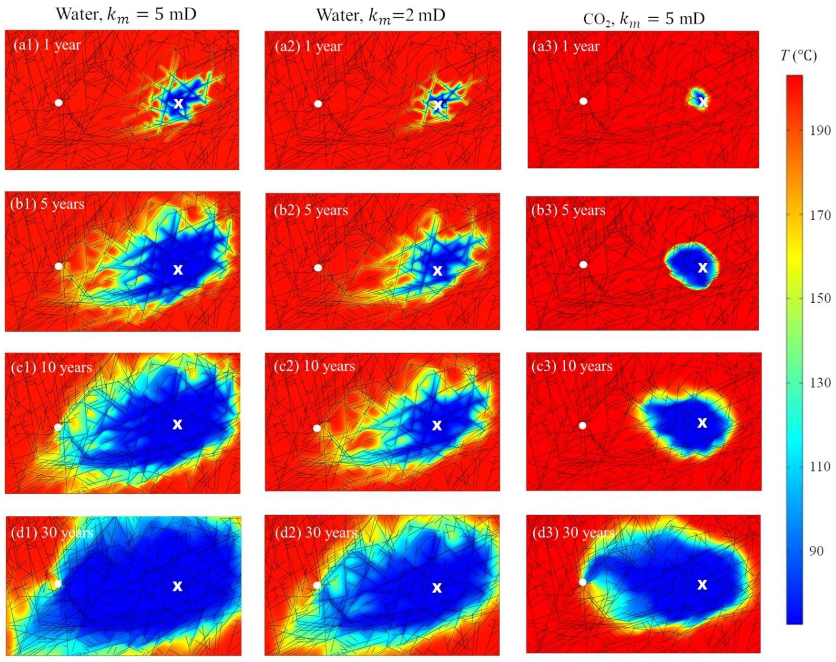
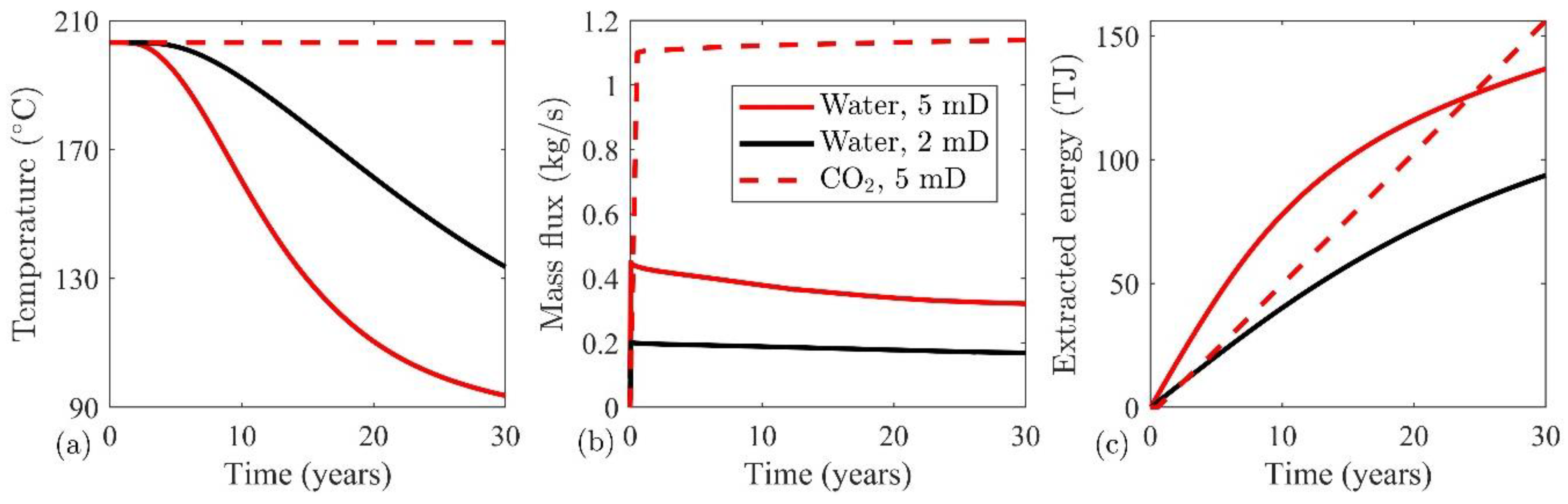
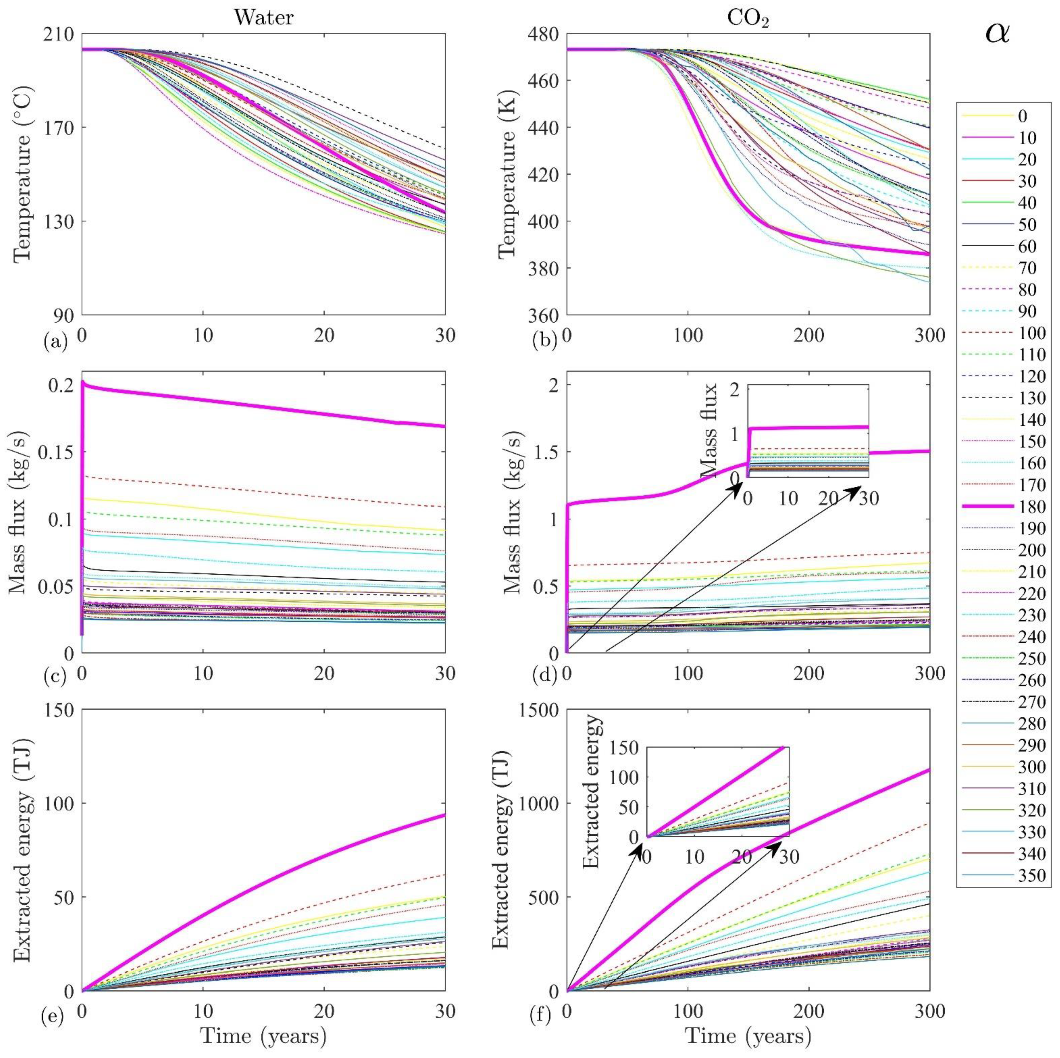
coupled THM mechanisms for heat mining using water as heat-carrying fluid,
(b)
coupled THM processes when CO2 is the heat-carrying fluid, and
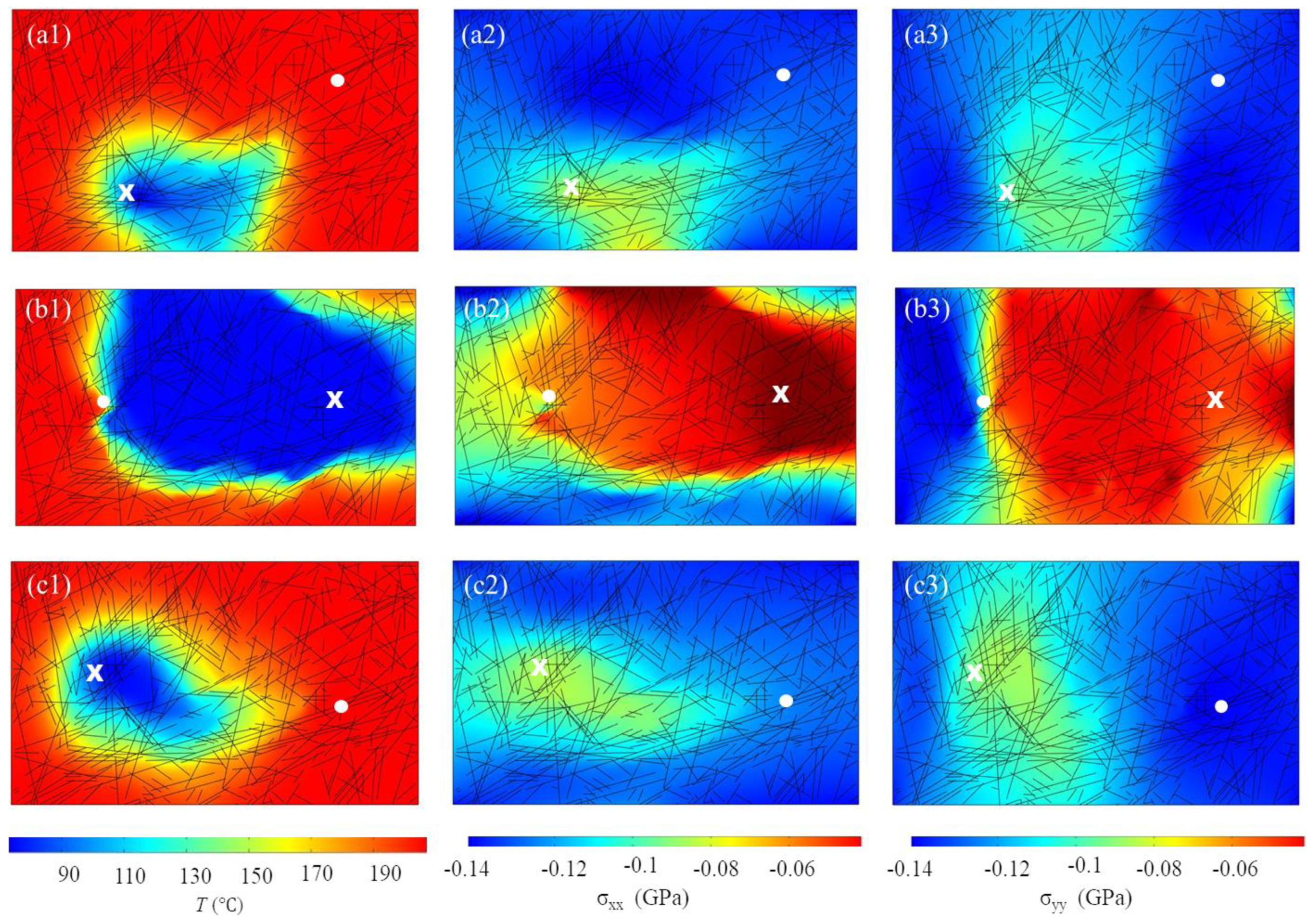
(c)
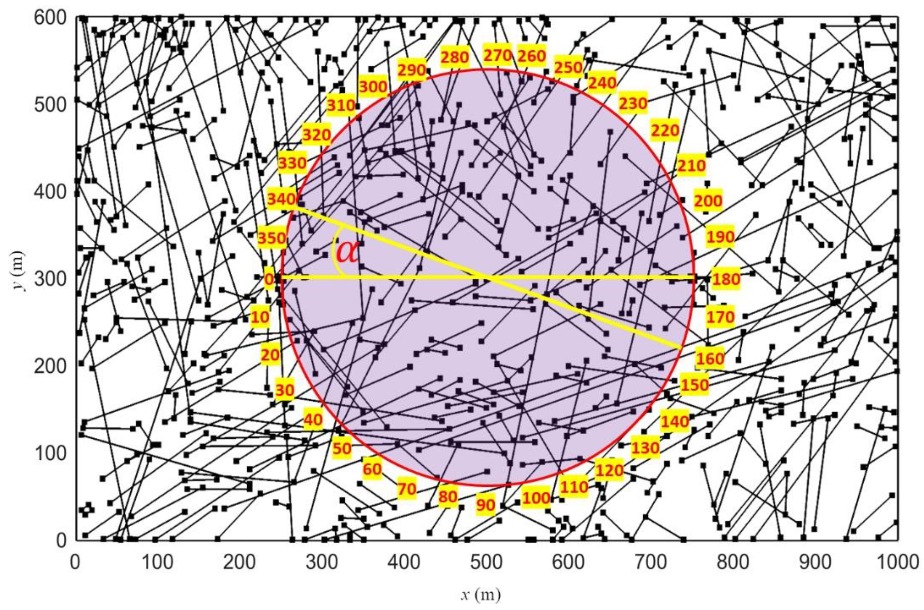
predicting a suitable doublet well position for a given fracture network to obtain highest mass flux from the production well and maximize the heat production.
The results are presented for two working fluids: water and CO2. Reservoir permeability of 2 mD and 5 mD are considered. These values are chosen in a way that sweep efficiency with the different working fluids to be similar at the same time.
Furthermore, permeability values are kept constant to understand the working fluid effect by running another case 180. Other parameters are listed in Table 1 that are not site specific and selected to represent a generic geothermal system, and the fracture map is the same for all scenarios. Constant injection and production pressures are considered at both the wellbores. A two-dimensional horizontal cross-sectional reservoir is considered for all the simulations.
We performed a mesh sensitivity analysis with case 180 for CO2 (it has the highest velocity variation, and the simulations convergence is the most complex among all the cases). Here, the mesh sensitivity analysis is attached for the simulations with (a) 92,655 domain elements and 12,103 boundary elements, (b) 112,818 domain elements and 13,071 boundary elements and (c) 181,410 domain elements and 15,687 boundary elements. Convergence was not achieved with the mesh size of the 71,089 domain elements and 10,357 boundary elements. The maximum element size for the standard case is (a) 67 m, (b) 37 m, and (c) 18 m, whereas the minimum element size is (a) 0.3 m, (b) 0.125 m, and (c) 0.075 m. The maximum element growth rate is (a) 1.3, (b) 1.25, and (c) 1.2, the curvature factor is (a) 0.3, (b) 0.25, and (c) 0.25, and the resolution of the narrow regions is 1 for all three cases. Free triangular meshes are used for discretizing this domain.
Based on this description, our results are insensitive to the mesh refinements (see Figure 3).
Figure 4 shows the time evolution of reservoir temperature distribution during the heat extraction operation using water and CO2 for case 180. Here, the injection well is present at 180, and the production well is present at 0 as shown in Figure 2. The reservoir permeability for the left (Figure 4(a1–d1)) and right (Figure 4(a3–d3)) columns is 5 mD whereas the middle column has 2 mD permeability (Figure 4(a2–d2)). Higher reservoir permeability in the case of the left column causes faster cold fluid propagation through the fracture network. Additionally, water propagation through the fractures becomes less dominant, and it starts flowing through the rock matrix at higher permeability as shown in Figure 4(c1,d1). We adopted smaller reservoir permeability for well placement when water is the working fluid to account for both these factors. The cold-water propagation is aligned along the dominant fracture rather than the horizontal axis between the doublet. The reason behind selecting different permeability values for water and CO2 is to reach a similar sweep efficiency with different fluids; however, we provided the quantitative comparison between simulation of water at 5 mD, 2 mD and CO2 at 5 mD for case 180 as shown in Figure 5. Figure 5a–c shows that CO2 is a better-working fluid concerning the breakthrough time, mass flux, and cumulatively extracted energy, respectively over 30 years.
The viscosity of supercritical CO2 at injection conditions is approximately half compared to water. Higher reservoir permeability and lower viscosity indicate CO2 propagation through the fractures as well as through the matrix rather than flowing through fractures only as seen in Figure 4(a2,b2). Figure 4(a3–d3) shows that the cold fluid plume spread is much diffusive compared to water, and flow is primarily occurring through the matrix. However, Figure 4(d3) shows that CO2 flows through the dominant fractures near the production well. Therefore, fluid propagation through the fractures is the principal mechanism between the doublet, which is assisted by flow through permeable rock matrix.
Furthermore, convective heat transfer inside the rock matrix and the fracture is the primary heat transfer mechanism. Therefore, the fractures control the heat transfer in a fractured reservoir. To show the relative importance of convective to conductive heat transfer, we calculated Peclet number ( P e ), a nondimensional number which indicates the ratio of convective to conductive heat transfer [49] and it can be written as P e = u L ρ i C p , i k i , where u is the fluid velocity, L is the characteristic length (here it is 500 m, the distance between the two wells), the subscript i indicates the fluid either water or CO2, ρ i is the fluid density, C p , i is the specific heat capacity of fluid and k i is the fluid thermal conductivity. Figure 6a shows the P e value after one year for the entire reservoir for case 180, where CO2 is the working fluid. To elaborate on the relative impact of convective heat transfer inside the fracture, one fracture is selected as shown in Figure 6b, and the corresponding P e number is shown in Figure 6c. P e number is estimated for five different times, and for all the cases, P e number is significantly larger than 1, indicating more vigorous convection than conduction.
Results obtained from the 36 reservoir simulations on the well positioning are shown in Figure 7. For water simulations, reservoir permeability is 2 mD, whereas, for cases with CO2 as working fluid, permeability is 5 mD. Water-based models demonstrate faster thermal breakthrough (Figure 7a) due to higher specific heat capacity than CO2. Therefore, water simulations are presented for 30 years whereas CO2 results are plotted for 300 years. We magnified the results for the CO2 over 30 years in Figure 7b,d,f to compare it with water (see Figure 7a,c,e). Figure 7a shows thermal drawdown at the production well when water is the working fluid. The fastest thermal drawdown was observed for case 220 (see Figure 8(c1)) whereas the slowest thermal drawdown occurred for case 130 (see Figure 8(a1)). From Figure 2, it is clear that case 220 has a well position along a dominant fracture supported by minor intersecting fractures, whereas case 130 wells are aligned approximately orthogonal to this prevalent fracture. Figure 8(a2,a3) show thermoelastic stress along the horizontal and vertical directions, respectively, indicating stress localization spans across the cold fluid plume region. Greater concentration of connected fractures in the area away from the doublet axis causes prolonged thermal breakthrough time. Therefore, in 30 years, the temperature drop is approximately 40 °C for case 130, whereas case 220 shows a 75 °C temperature drop at the production well.
In comparison to water, CO2 has approximately seven times smaller thermal conductivity at the injection conditions. Due to this, thermal depletion time is prolonged when CO2 is the working fluid compared to water as the heat-carrying fluid. Figure 7b shows the thermal drawdown at the production well when CO2 is the operating fluid. It shows that the thermal drawdown curves depend significantly on the fracture network connectivity than water. The slowest thermal drawdown is demonstrated by case 40, where production well temperature drops by approximately 20 °C in 300 years. In contrast, the fastest thermal drawdown is displayed by case 180, where around 90 °C temperature drop is estimated. Figure 9(a1,a2) show reservoir temperature distribution for case 40 and case 180, respectively. In Figure 9(a1), the cold fluid spread is extremely slow since a high fracture density is present near point 40, as shown in Figure 2 that is present away from the doublet axis. This leads to a reduced amount of cold fluid injection and restricted heat exchange between the fluid–fractures and fluid–matrix in the reservoir, decreasing the horizontal and vertical thermoelastic stress as shown in Figure 9(a2,a3), respectively. A detailed sensitivity analysis of dependent parameters is performed for water [47] and CO2 [50] based geothermal systems for the same fractured reservoir as mentioned in this paper. Our numerical simulations consider poroelastic stress, but we have not shown here that they contribute little due to the fluid injection and production, as shown in our previous findings [47,50]. For case 180, Figure 9(b1) shows reservoir temperature distribution after 300 years. It indicates that the hot fluid has been completely extracted between the doublet, and the heat replenishment is too slow to recharge this depleting heat content. Figure 9(b2,b3) approves this reasoning that due to favorable fracture density along the doublet axis, higher fluid flux reinjection results in higher thermoelastic stress evolution.
Figure 7c,d show mass flux at the production well for 36 cases when the working fluid in the reservoir is water and CO2, respectively. The mass flux for CO2 is approximately five times higher than water to compensate for smaller viscosity and higher permeability by maintaining the reservoir injection pressure. For both the fluids highest mass flux is observed for case 180, and the smallest mass flux is marked for case 350. Even though these two doublet arrangements have approximately the same axis (endpoints of a single line connecting injection and production wells), the fracture density near the production well plays a crucial role in mass flux; a similar observation was made by Zhang et al. [2]. For case 180, fractures are well connected near the production well, which assists in higher fluid production, whereas in the case of 350, fractures are not connected in a wide area leading to smaller fluid production. The temperature front in Figure 8(e1) shows the weak convective flow for case 350. This can be easily seen from the stress distribution plots in Figure 8(e2,e3) for case 350 when water is the working fluid and in Figure 9(c2,c3) for case 350 when CO2 is the working fluid. The decrease in mass flux for all the cases with time is due to a in water viscosity with increased fluid temperature. However, we observe that the mass flux increases with time if CO2 is the working fluid. This increase is approximately <30% between the period when CO2 production starts till 300 years of numerical simulation. This increase is pronounced for the case 180 where we observe that the mass flux increases from 1.15 to 1.5 kg/s and the increase starts after approximately 50 years from the beginning of the operation. This discrepancy is observed due to limitations in the equation of state used in modeling using COMSOL Multiphysics. Since viscosity is a function of temperature only, the mass flux increase is observed after the breakthrough time (see Equation (11)).
The energy extraction potential from the reservoir for both the fluids are approximately the same (see Figure 7e,f) since in the case of water simulations, reservoir permeability is 2.5 times more negligible compared to CO2, and the mass flux of CO2 is approximately 3–5 times greater than water. In contrast, the specific heat capacity of water is around three times higher compared to CO2 with three times higher viscosity. Due to higher mass flux and delayed thermal drawdown operation, total energy extraction potential is significantly higher when CO2 is the working fluid. Case 180 for both the fluids shows the highest energy extraction potential due to the maximum mass flow rate in Figure 8(b1–b3). However, due to higher mass flux, thermal depletion is also fastest, and therefore, doublet placed for case 180 may not show a longer operation when water is the working fluid. Case 250 for water and case 350 for CO2 show the least energy extraction potential over 30 and 300 years, respectively. Figure 8(d1) shows the reservoir temperature distribution for case 250 when water is used for heat transmission. It is visible from Figure 8d1 that a more incredible amount of cold fluid is present near the injection well, and there is only one large fracture along the doublet axis. This limits the fluid transmission at a higher rate only through a narrow region causing limited energy extraction.
Furthermore, Figure 8(d2,d3) shows the corresponding stress distribution for the horizontal and vertical directions. On the other hand, Figure 9(c1) shows reservoir temperature distribution for case 350 and CO2 is used as working fluid and localization of cold fluid near the injection well in the absence of any dominating fracture system. The passage of fluid is limited through the fractures toward the production well. The stress field in Figure 8(c2,c3) shows the horizontal and vertical stress are well aligned with the temperature propagation. However, since thermal breakthrough is slower when CO2 is used for heat transmission, energy extraction potential may enhance if EGS operation is performed beyond 300 years.

4. Conclusions

Geothermal energy extraction from deep fractured reservoirs can support high energy demand for a long duration. Water and CO2 are two fluids that can extract energy from the subsurface. A fractured reservoir shows a complex network of fractures, and fracture conductivity controls the primary fluid passage for heat extraction longevity of the operation. Well placement for a given fracture network should consider the fracture density and orientation. Keeping all the parameters constant except the injection–production doublet axis orientation, we observe a difference of approximately ten times of energy extracted among the studied cases. High fracture density in the vicinity of the production well is the reason behind this increased energy extraction. The doublet axis orientation affects the injectivity (poroelastic stress) and temperature propagation (thermoelastic stress). It has a great impact on the stress field development during heat extraction.
Fluid type plays a significant role in determining the THM behavior of the EGS. The viscosity of fluid determines the temperature propagation through the fractures, as well as through the rock matrix. CO2 with lower viscosity can penetrate easily inside the matrix zone. This effect, combined with the lower specific heat capacity of CO2, eventuates the cold front of fluid propagation through the matrix and fracture. While water with high viscosity and specific heat capacity mainly transmits heat alongside the fracture and results in early breakthrough time. Different cases with water have a small range of breakthrough time compared to CO2. While CO2 shows a higher flow rate, resulting from the lower viscosity, this behavior is compensated by the higher heat capacity of water. Therefore, the overall heat extraction is comparable for both fluids.

Author Contributions

Conceptualization, S.M. and M.S.; methodology, S.M. and M.S.; software, S.M. and M.S.; validation, S.M. and M.S. writing—original draft preparation, S.M. and M.S.; writing—review and editing, K.B.; visualization, S.M. and M.S.; supervision, K.B. and I.S.; project administration, K.B.; funding acquisition, K.B. All authors have read and agreed to the published version of the manuscript.

Funding

The work is conducted as part of the MEET project that has received funding from the European Union’s Horizon 2020 research and innovation programme under grant agreement No 792037.

Data Availability Statement

Data used in this paper are synthetic and can be reproduced from the Table 1.

Acknowledgments

Group of Geothermal Science and Technology, Institute of Applied Geosciences, Technische Universität Darmstadt has provided institutional support to authors. Authors would like to acknowledge anonymous reviewers for their valuable comments and suggestions.

Conflicts of Interest

The authors declare no conflict of interest.

Appendix A

Table A1. List of parameters.
SymbolParameter
p Fluid pressure
T Fluid Temperature
ε V Pore volumetric strain
α m Biot’s coefficient of porous media
α f Biot’s coefficient of the fracture
ϕ m Reservoir porosity
ϕ f Fracture zone porosity
S m Storage coefficients of fluid
S 1 Storage coefficients of rock matrix
S f Storage coefficients of fracture
β 1 Thermal expansion coefficients of fluid
β m Thermal expansion coefficients of rock matrix
β f Thermal expansion coefficient of fracture
ρ   &   ρ 1 Fluid density
k m pressure-dependent rock matrix permeability
k f stress-dependent fracture permeability
e h hydraulic aperture between two fracture surfaces
n Q m n . ( ρ k m μ p ) , mass flux exchange between porous media and the fracture
T Gradient operator restricted to the fracture’s tangential plane
T m Rock matrix temperature
T l Fluid temperature
ρ m Rock density
C p , m Specific heat capacity of the rock matrix
λ m Heat conductivity of the rock matrix
q m l Rock matrix-pore fluid interface heat transfer coefficient
ρ f density of the fracture zone
C p , f Specific heat capacity of the fracture
λ f Heat conductivity of the fracture
q f l Rock fracture-fluid interface heat transfer coefficient
C p   &   C p , l Heat capacity of the fluid at a constant pressure
λ l Heat conductivity of the fluid
σ i j Total stress
G & λ Lame’s constants
trTrace operator
K 2 G ( 1 + ν ) 3 ( 1 2 ν ) , bulk modulus of the drained porous media
β T Volumetric thermal expansion coefficient of porous media
δ i j Dirac dealt function
α p Biot’s coefficient
σ e f f i j Effective stress
f i External body force
Δ e n Change in the initial aperture of the fracture under in-situ stresses
e 0 Initial aperture of the fracture
σ e f f n Effective normal stress acting on the fracture surface
σ n r e f Effective normal stress required to cause 90% reduction in fracture aperture
μ CO2 dynamic viscosity
κ CO2 thermal conductivity

References

  1. Singh, M.; Tangirala, S.K.; Chaudhuri, A. Potential of CO2 based geothermal energy extraction from hot sedimentary and dry rock reservoirs, and enabling carbon geo-sequestration. Geomech. Geophys. Geo-Energy Geo-Resour. 2020, 6, 16. [Google Scholar] [CrossRef]
  2. Zhang, H.; Huang, Z.; Zhang, S.; Yang, Z.; Mclennan, J.D. Improving heat extraction performance of an enhanced geothermal system utilizing cryogenic fracturing. Geothermics 2020, 85, 101816. [Google Scholar] [CrossRef]
  3. Stefansson, V. Geothermal reinjection experience. Geothermics 1997, 26, 99–139. [Google Scholar] [CrossRef]
  4. Mahmoodpour, S.; Singh, M.; Turan, A.; Bär, K.; Sass, I. Hydro-Thermal Modeling for Geothermal Energy Extraction from Soultz-sous-Forêts, France. Geosciences 2021, 11, 464. [Google Scholar] [CrossRef]
  5. Hofmann, H.; Babadagli, T.; Zimmermann, G. Hot water generation for oil sands processing from enhanced geothermal systems: Process simulation for different hydraulic fracturing scenarios. Appl. Energy 2014, 113, 524–547. [Google Scholar] [CrossRef]
  6. Hofmann, H.; Babadagli, T.; Yoon, J.S.; Blöcher, G.; Zimmermann, G. A hybrid discrete/finite element modeling study of complex hydraulic fracture development for enhanced geothermal systems (EGS) in granitic basements. Geothermics 2016, 64, 362–381. [Google Scholar] [CrossRef]
  7. Lepillier, B.; Daniilidis, A.; Gholizadeh, N.D.; Bruna, P.-O.; Kummerow, J.; Bruhn, D. A fracture flow permeability and stress dependency simulation applied to multi-reservoirs, multi-production scenarios analysis. Geotherm. Energy 2019, 7, 24. [Google Scholar] [CrossRef]
  8. Baujard, C.; Genter, A.; Dalmais, E.; Maurer, V.; Hehna, R.; Rosillettea, R.; Vidal, J.; Schmittbuhl, J. Hydrothermal characterization of wells GRT-1 and GRT-2 in Rittershoffen, France: Implications on the understanding of natural flow systems in the rhine graben. Geothermics 2017, 65, 255–268. [Google Scholar] [CrossRef] [Green Version]
  9. Islam, J.; Vasant, P.M.; Negash, B.M.; Laruccia, M.B.; Myint, M. Watada A holistic review on artificial intelligence techniques for well placement optimization problem. Adv. Eng. Softw. 2020, 141, 102767. [Google Scholar] [CrossRef]
  10. Zhang, L.; Deng, Z.; Zhang, K.; Long, T.; Desbordes, J.K.; Sun, H.; Yang, Y. Well-placement optimization in an enhanced geothermal system based on the fracture continuum method and 0–1 programming. Energies 2019, 12, 709. [Google Scholar] [CrossRef] [Green Version]
  11. Ansari, E.; Hughes, R.; White, C.D. Well placement optimization for maximum energy recovery from hot saline aquifers. In Proceedings of the Thirty-Ninth Workshop on Geothermal Reservoir Engineering, Stanford University, Stanford, CA, USA, 24–26 February 2014. [Google Scholar]
  12. Yousefzadeh, R.; Sharifi, M.; Rafiei, Y. An efficient method for injection well location optimization using Fast Marching Method. J. Pet. Sci. Eng. 2021, 204, 108620. [Google Scholar] [CrossRef]
  13. Bangerth, W.; Klie, H.; Wheeler, M.; Stoffa, P.; Sen, M. On optimization algorithms for the reservoir oil well placement problem. Comput. Geosci. 2006, 10, 303–319. [Google Scholar] [CrossRef]
  14. Onwunalu, J.E.; Durlofsky, L.J. Application of a particle swarm optimization algorithm for determining optimum well location and type. Comput. Geosci. 2010, 14, 183–198. [Google Scholar] [CrossRef]
  15. Forouzanfar, F.; Li, G.; Reynolds, A.C. A two-stage well placement optimization method based on adjoint gradient. In Proceedings of the SPE Annual Technical Conference and Exhibition, Florence, Italy, 20–22 September 2010. [Google Scholar]
  16. Sarma, P.; Durlofsky, L.J.; Aziz, K. Computational techniques for closed–loop reservoir modeling with application to a realistic reservoir. Petrol. Sci. Technol. 2008, 26, 1120–1140. [Google Scholar] [CrossRef]
  17. Zandvliet, M.; Handels, M.; Essen, G.; Brouwer, R.; Jansen, J. Adjoint-based well-placement optimization under production constraints. SPE J. 2008, 13, 392–399. [Google Scholar] [CrossRef]
  18. Vaseghi, F.; Ahmadi, M.; Sharifi, M.; Vanhoucke, M. Generalized multi-scale stochastic reservoir opportunity index for enhanced well placement optimization under uncertainty in green and brownfields. Oil Gas Sci. Technol.—Rev. IFP Energ. Nouv. 2021, 76, 41. [Google Scholar] [CrossRef]
  19. Chen, J.; Jiang, F. Designing multi-well layout for enhanced geothermal system to better 489 exploit hot dry rock geothermal energy. Renew. Energy 2015, 74, 37–48. [Google Scholar] [CrossRef]
  20. Kong, Y.; Pang, Z.; Shao, H.; Kolditz, O. Optimization of well-doublet placement in geothermal reservoirs using numerical simulation and economic analysis. Environ. Earth Sci. 2017, 76, 118. [Google Scholar] [CrossRef]
  21. Liang, X.; Xu, T.; Feng, B.; Jiang, Z. Optimization of heat extraction strategies in fault-controlled hydro-geothermal reservoirs. Energy 2018, 164, 853–870. [Google Scholar] [CrossRef]
  22. Babaei, M.; Nick, H.M. Performance of low-enthalpy geothermal systems: Interplay of spatially correlated heterogeneity and well-doublet spacings. Appl. Energy 2019, 253, 113569. [Google Scholar] [CrossRef]
  23. Jiang, Z.; Xu, T.; Wang, Y. Enhancing heat production by managing heat and water flow in confined geothermal aquifers. Renew. Energy 2019, 142, 684–694. [Google Scholar] [CrossRef]
  24. Blank, L.; Rioseco, E.M.; Caiazzo, A.; Wilbrandt, U. Modeling, simulation, and optimization of geothermal energy production from hot sedimentary aquifers. Comput. Geosci. 2021, 25, 67–104. [Google Scholar] [CrossRef]
  25. Chen, S.-Y.; Hsieh, B.-Z.; Hsu, K.-C.; Chang, Y.-F.; Liu, J.-W.; Fan, K.-C.; Chiang, L.-W.; Han, Y.-L. Well spacing of the doublet at the Huangtsuishan geothermal site, Taiwan. Geothermics 2021, 89, 101968. [Google Scholar] [CrossRef]
  26. Zhang, S.; Jiang, Z.; Zhang, S.; Zhang, Q.; Feng, G. Well placement optimization for large-scale geothermal energy exploitation considering nature hydro-thermal processes in the Gonghe Basin, China. J. Clean. Prod. 2021, 317, 128391. [Google Scholar] [CrossRef]
  27. Akin, S.; Kok, M.V.; Uraz, I. Optimization of well placement geothermal reservoirs using artificial intelligence. Comput. Geosci. 2010, 36, 776–785. [Google Scholar] [CrossRef]
  28. Samin, M.Y.; Faramarzi, A.; Jefferson, I.; Harireche, O. A hybrid optimization approach to improve long-term performance of enhanced geothermal system (EGS) reservoirs. Renew. Energy 2019, 134, 379–389. [Google Scholar] [CrossRef] [Green Version]
  29. Gudmundsdottir, H.; Horne, R.N. Inferring interwell connectivity in fractured geothermal reservoirs using neural networks. In Proceedings of the World Geothermal Congress 2020+1, Reykjavik, Iceland, 24–27 October 2021. [Google Scholar]
  30. Pandey, S.N.; Singh, M. Artificial neural network to predict the thermal drawdown of enhanced geothermal system. J. Energy Resour. Technol. 2021, 143, 010901. [Google Scholar] [CrossRef]
  31. Ishitsuka, K.; Kobayashi, Y.; Watanabe, N.; Yamaya, Y.; Bjarkson, E.; Suzuki, A.; Mogi, T.; Asanuma, H.; Kajiwara, T.; Sugimoto, T.; et al. Bayesian and neural network approached to estimate deep temperature distribution for assessing a supercritical geothermal system: Evaluation using a numerical model. Nat. Resour. Res. 2021, 30, 3289–3314. [Google Scholar] [CrossRef]
  32. Chen, M.; Tompson, A.F.B.; Mellors, R.J. Abdalla An efficient optimization of well placement and control for geothermal prospect under geological uncertainty. Appl. Energy 2015, 137, 352–363. [Google Scholar] [CrossRef] [Green Version]
  33. Zhang, W.; Qu, Z.; Guo, T.; Wang, Z. Study of the enhanced geothermal system (EGS) heat mining from variably fractured hot dry rock under thermal stress. Renew. Energy 2019, 143, 855–871. [Google Scholar] [CrossRef]
  34. Gao, X.; Zhang, Y.; Huang, Y.; Ma, Y.; Zhao, Y.; Liu, Q. Study on heat extraction considering the number and orientation of multilateral wells in a complex fractured geothermal reservoir. Renew. Energy 2021, 177, 833–852. [Google Scholar] [CrossRef]
  35. Aliyu, M.D.; Chen, H.-P.; Harireche, O. Finite element modeling for productivity of geothermal reservoirs via extraction well. In Proceedings of the 24th UK conference of the Association for Computational Mechanics in Engineering, Cardiff University, Cardiff, UK, 31 March–1 April 2016; pp. 331–334. [Google Scholar]
  36. Aliyu, M.D.; Chen, H.-P. Optimum control parameters and long-term productivity of geothermal reservoirs using coupled thermo-hydraulic process modeling. Renew. Energy 2017, 112, 151–165. [Google Scholar] [CrossRef]
  37. Brown, D. A hot dry rock geothermal energy concept utilizing supercritical CO2 instead of water. In Proceedings of the 25th Workshop on Geothermal Reservoir Engineering, Stanford University, Stanford, CA, USA, 24–26 January 2000; p. SGP-TR-165. [Google Scholar]
  38. Isaka, B.A.; Ranjith, P.; Rathnaweera, T. The use of supercritical carbon dioxide as the working fluid in enhanced geothermal systems (EGSs): A review study. Sustain. Energy Technol. Assess 2019, 36, 100547. [Google Scholar]
  39. Atrens, A.D.; Gurgenci, H.; Rudolph, V. Electricity generation using a carbon-dioxide thermosiphon. Geothermics 2010, 39, 161–169. [Google Scholar] [CrossRef]
  40. Bongole, K.; Sun, Z.; Yao, J.; Mehmood, A.; Yueying, W.; Mboje, J.; Xin, Y. Multifracture response to supercritical CO2- EGS and water-EGS based on thermo-hydro-mechanical coupling method. Int. J. Energy Res. 2019, 43, 7173–7196. [Google Scholar]
  41. Atrens, A.D.; Gurgenci, H.; Rudolph, V. CO2 thermosiphon for competitive geothermal power generation. Energy Fuels 2009, 23, 553–557. [Google Scholar] [CrossRef]
  42. Tran, N.H.; Chen, Z.; Rahman, S.S. Object-based global optimization in modeling discrete-fracture network map: A case study. In Proceedings of the SPE Annual Technical Conference and Exhibition, Denver, CO, USA, 5–8 October 2003; p. 84456. [Google Scholar]
  43. COMSOL Multiphysics® v. 5.5. COMSOL AB, Stockholm, Sweden. Available online: www.comsol.com (accessed on 11 November 2020).
  44. Barton, N.; Bandis, S.; Bakhtar, K. Strength, deformation and conductivity coupling of rock joints. Int. J. Rock Mech. Min. Sci. Geomech. Abstr. 1985, 22, 121–140. [Google Scholar] [CrossRef]
  45. Bandis, S.C.; Lumsden, A.C.; Barton, N.R. Fundamentals of rock joint deformation. Int. J. Rock Mech. Min. Sci. Geomech. Abstr. 1983, 20, 249–268. [Google Scholar] [CrossRef]
  46. Bai, B. One-dimensional thermal consolidation characteristics of geotechnical media under non-isothermal condition. Eng. Mech. 2005, 22, 186–191. [Google Scholar]
  47. Mahmoodpour, S.; Singh, M.; Turan, A.; Bär, K.; Sass, I. Key parameters affecting the performance of fractured geothermal reservoirs: A sensitivity analysis by thermo-hydro-mechanical simulation. arXiv 2021, arXiv:2107.02277. [Google Scholar]
  48. Bär, K.; Reinsch, T.; Bott, J. P3-PetroPhysical Property Database. V. 1.0. GFZ Data Services. 2019. Available online: https://doi.org/10.5880/GFZ.4.8.2019.P3 (accessed on 1 April 2021).
  49. Bergman, T.L.; Lavine, A.S.; Incropera, F.P. Fundamentals of Heat and Mass Transfer, 7th ed.; John Wiley & Sons, Incorporated: Hoboken, NJ, USA, 2011; ISBN 9781118137253. [Google Scholar]
  50. Mahmoodpour, S.; Singh, M.; Bär, K.; Sass, I. Thermo-hydro-mechanical modeling of an Enhanced geothermal system in a fractured reservoir using CO2 as heat transmission fluid—A sensitivity investigation. arXiv 2021, arXiv:2108.05243. [Google Scholar]
Figure 1. An enhanced geothermal system. The subsurface plan shows an intricate network of fractures. For optimized power generation, appropriate placement of the injection and production wells is necessary.
Geosciences 12 00019 g001
Figure 2. The geometry of the reservoir. Injection and production wells are placed 500 m apart. Total 36 cases or 36 values of α are considered for simulations. Here, when the injection well is present at 0 and production well is present at 180 and they are 500 m placed apart, the value of α is 0. When the injection well is present at 340 and the production well is present at 160, the value of α is 340.
Geosciences 12 00019 g002
Figure 3. Mesh sensitivity results for three different number of mesh elements.
Geosciences 12 00019 g003
Figure 4. Reservoir temperature distribution at time 1 year (a1a3), 5 years (b1b3), 10 years (c1c3) and 30 years (d1d3) when the injection well is present at 180 and the production well is placed at 0. Results from water for reservoir permeability 5 mD and 2 mD are shown by (a1d1) and (a2d2) respectively. CO2 as working fluid results are displayed in (a3d3). The reservoir permeability for CO2 simulations is 5 mD. The injection wellbore position is shown by cross symbol whereas a circle indicates production wellbore position.
Geosciences 12 00019 g004
Figure 5. Comparison of working fluid effects, (a) temperature at the production well, (b) mass flux of different fluid, and (c) extracted energy.
Geosciences 12 00019 g005
Figure 6. For case 180 and CO2 as the working fluid after one year, (a) Peclet number distribution across the reservoir, (b) fracture considered for estimating fracture length, and (c) Peclet number along with the fracture length.
Geosciences 12 00019 g006
Figure 7. The temperature at the production well for (a) water and (b) CO2, mass flux at the production well for (c) water and (d) CO2, and cumulative energy extraction using (e) water and (f) CO2 as heat-carrying fluid. Results from 36 simulation cases are plotted as shown by the legend, and case 180 is indicated by bold magenta color. Here Case 180 means injection well is present at 180, and production well is present at 0 (see Figure 2).
Geosciences 12 00019 g007
Figure 8. Distribution of (a1e1) reservoir temperature, (a2e2) horizontal thermoelastic stress and (a3e3) vertical thermoelastic stress when water is used as the working fluid. Here Case 130 is displayed by (a1a3), Case 180 is displayed by (b1b3), Case 220 is displayed by (c1c3), Case 250 is displayed by (d1d3), and Case 350 is displayed by (e1e3). All contours are plotted at ten years. The injection wellbore position is shown by cross symbol whereas a circle indicates production wellbore position.
Geosciences 12 00019 g008
Figure 9. Distribution of (a1c1) reservoir temperature, (a2c2) horizontal thermoelastic stress and (a3c3) vertical thermoelastic stress when CO2 is used as the working fluid. Here Case 40 is displayed by (a1a3), Case 180 is displayed by (b1b3), and Case 350 is displayed by (c1c3). All contours are plotted at 100 years. The injection wellbore position is shown by cross symbol whereas a circle indicates production wellbore position.
Geosciences 12 00019 g009
Table 1. Numerical simulation parameters (see the range of database in [48]).
ParameterMagnitude for Water-Based SimulationsMagnitude for CO2 Based Simulations
Young’s modulus 40   GPa 40   GPa
Poisson’s ratio 0.25 0.25
Rock density 2500   kg m 3 2500   kg m 3
Horizontal stress 50   MPa 50   MPa
Vertical stress 50   MPa 50   MPa
Initial pressure 30   MPa 30   MPa
Injection pressure 50   MPa 50   MPa
Rock porosity 0.2 0.2
Rock permeability 2   mD 5   mD
Fracture zone porosity 0.5 0.5
Fracture roughness 1 1
Fracture aperture 0.2   mm 0.2   mm
Closure stress 150   MPa 150   MPa
Wellbore radius 0.2   m 0.2   m
Rock thermal conductivity 3   W m × K 3   W m × K
Fracture zone thermal conductivity 2.5 W m × K 2.5 W m × K
Rock specific heat capacity 800 J kg × K 800 J kg × K
Fracture zone specific heat capacity 800 J kg × K 800 J kg × K
Initial temperature 200   ° C 200   ° C
Biot coefficient 0.7 0.7
Thermal expansion coefficient 10 5 1 K 10 5 1 K
Injection temperature 70   ° C 70   ° C
Publisher’s Note: MDPI stays neutral with regard to jurisdictional claims in published maps and institutional affiliations.

