Identification of Near-Fault Impulsive Signals and Their Initiation and Termination Positions with Convolutional Neural Networks

Abstract

Ground motions recorded in near-fault regions may contain pulse-like traces in the velocity domain. Their long periodicity can identify such signals with large amplitudes. Impulsive signals can be hazardous for buildings, creating large demands due to their long periods. In this study, a dataset was collected from various data centres. Initially, all the impulsive signals, which are in reality rare, are manually identified. Furthermore, then, synthetic velocity waveforms are created to increase the number of impulsive signals by using the model developed by Mavroeidis and Papageorgiou, and $k^{-2}$ kinematic modelling. In accordance, a convolutional neural network (CNN) was trained to detect impulsive signals by using these synthetic impulsive signals and ordinary signals. Furthermore, manually labelled impulsive signals are used to detect the initiation and the termination positions of impulsive signals. To do so, the velocity waveform and position and amplitude information of the maximum and minimum points are used. Once the model detects the positions, the period of the pulse is calculated by analysing spectral periods. Although our detection algorithm works relatively worse than three robust algorithms used for benchmarks, it works significantly better in the determination of initiation and termination positions. At this moment, our models understand the features of the impulsive signals and detect their location without using any thresholds or any formulations that are heavily used in previous studies.

1. Introduction

The increasing number of seismic stations near the active fault lines has allowed the investigation of near-fault seismic features of earthquakes. The characteristics of the signals recorded in near-fault regions on large-magnitude earthquakes are the interest of both classical and engineering seismology due to the presence of large-amplitude velocity time histories, with long periods in particular cases (e.g., Baltzopoulos et al. [1]). These signals are called impulsive signals. The directivity effect is one of the major causes of such signals [2]. It can be explained as the propagation of the rupture front to the site with the similar shear wave velocity of the medium in which the earthquake rupture propagates. When the directivity effect is present at the site of interest, most of the energy of the earthquake would be focused on a single or several periodic signals on velocity records. The directivity effect can be visible on both fault normal [3,4] and fault parallel sites [5,6] depending on the fault type. The fling step effect, which is the permanent displacement at the site of interest, is the second source of impulsive signals [7]. Shallow soil effects may also create impulsive signals. The basin effect focuses the seismic energy to a certain location, which creates an impulsive signal [8]. Loose soils also create impulsive signals [6]. Since the shallow soil effects depend on the local geology of the site of interest, they cannot be formalised as directivity or fling step effects. The effects that may damage the structures can be as follows:

• spectral ratios can be locally amplified in the region where the fundamental structural period is closer to the pulse period [9];
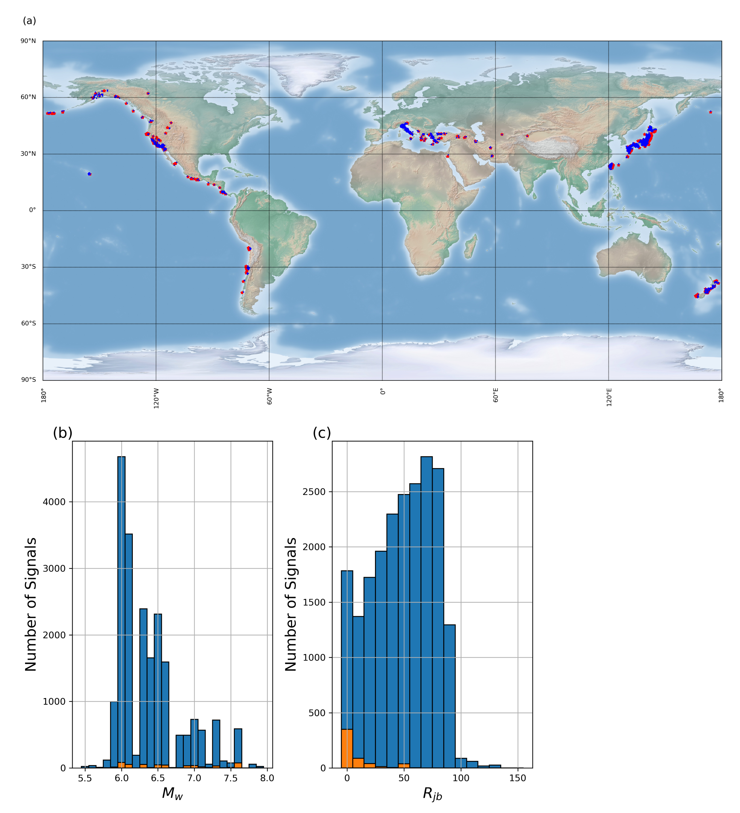
• the structure will be loaded with considerable seismic energy in few pulses in the higher modes [7,10,11,12].

Impulsive signals can be destructive to various types of structures, such as idealised single and multi degree-of-freedom systems [13], seismically isolated structures [14], and bridges [15]. Because of their hazardous effects on structures, it is vital to detect impulsive signals. Detecting impulsive signals makes it possible to calculate their probability of occurrence [16,17,18]. Thus, the effects of impulsive signals can be implemented into hazard maps [19].

Various methods have been developed to identify impulsive signals. Mavroeidis and Papageorgiou [20] used Gabor wavelets for the identification. Baker [21], on the other hand, used fourth-order Daubechies wavelets. A pulse identifier (PI) is developed for the identification process, which is a mathematical formula with a combination of various ratios and constants. Shahi and Baker [17] improved the study of Baker [21] with new data and created a new PI. Chang et al. [22] used energy-based classification using the energy ratio around the peak ground velocity (PGV) location and the total energy of the signal. Ertuncay and Costa [23] used Ricker and Morlet wavelets to analyse and determine impulsive signals. An energy-based classification is implemented in both the velocity time history and wavelet power spectrum. Different decision-making criteria have created disagreements on the characterisation of the signals.

Machine learning (ML) algorithms require a vast amount of data to understand the nature of the given problem. Thanks to the large set of waveforms recorded by the stations of national and international data centres, large datasets, such as Stanford Earthquake Dataset (STEAD) database of Mousavi et al. [24], are created. ML algorithms have enough data to understand the features of various seismological problems. With the help of a large amount of data, Meier et al. [25] differentiate noise from earthquakes, and Mousavi et al. [26], Ross et al. [27,28] detect P and S wave arrivals of the earthquakes along with the polarity detection of the first motion. Titos et al. [29] used recurrent neural networks, long short-term memory, and a gated recurrent unit to detect and classify continuous sequences of volcano-seismic events at the Deception Island Volcano, Antarctica. Titos et al. [30] evaluated the classification performance on seven different classes of isolated seismic events by using two different deep neural networks. Furthermore, ML can calculate the station-based magnitude of earthquakes Mousavi and Beroza [31].

In this study, we try to solve two problems, which are the detection of impulsive signals and their initiation and termination positions. For the first problem, two CNN models are trained using both synthetic and real data. Features of the real and synthetic data are explained Section 2. Features of the CNN are given in Section 3, and the outcomes of the CNN models are discussed in Section 4. For determining if a signal is impulsive or non-impulsive, a procedure is developed based on information from previous methods and a manual inspection. To measure the success of the model, the false positive (FPR) and false negative (FNR) rates were observed. We would like to minimise the rates to ensure that our model can detect impulsive signals with high accuracy. We want to reduce the FPR to ensure that our model is not giving false alarms; in this case, it is a non-impulsive signal. Furthermore, we also want to minimise the FNR as much as possible to have a model that labels the impulsive signals correctly. Our aim is to overcome the disagreements among previous studies by creating a generalised CNN model, and to do that, manual detection of impulsive signals is chosen. This approach is used by Baker [21], Mavroeidis and Papageorgiou [20], and Somerville [32] to create an empirical relation between the moment magnitude ($M_w$) and pulse period and generalise the features of impulsive signals. The same approach is implemented, and the waveforms are inspected visually. Accordingly, manually detected impulsive signals are used to validate our model. To understand the performance of our model, we not only compare it with manually inspected signals but also with identification results of the same signals by recently developed algorithms.

For the second problem, only the manually detected impulsive signals are used along with their initiation and termination positions. To understand the performance of the model, three parameters are defined, which are the mean squared error (MSE), the mean absolute error (MAE), and the coefficient of determination ($R^2$). We try to minimise the error while maximising the determination coefficient, and then, the performance of our model was compared with the previous studies. After the determination of the impulsive part, the period of the impulsive signal is determined. Spectral amplitudes and periods are used for the determination of the period. Periods determined by previous methods and our model are also compared. Several signals with a large difference in terms of the period are analysed individually.

2. Data

To train the CNN model efficiently, a dataset is created by collecting waveforms from the NGA-West 2 [33] database and national data centres from Canada, Chile, Costa Rica, Greece, Italy, Japan, Mexico, New Zealand, the United States of America, Taiwan, and Turkey. Crustal earthquakes are collected from various data centres. Earthquake data from strong-motion and broad-band stations are collected (Figure 1a). Earthquakes with a $M_w$ bigger than 5.5 with a hypocentral depth smaller than 55 $\mathrm{k}\mathrm{m}$ are chosen. Stations with epicentral distance less than 150 $\mathrm{k}\mathrm{m}$ are used.

The stations with two horizontal components were chosen, and the orientations were changed from North–South and East–West to fault normal and fault parallel since the directivity effect can be seen more easily in the fault-normal component [2,34]. Later studies show that impulsive signals may also occur in other orientations [9]. Vertical stations are also used. If a station does not have both of its horizontal components, only the vertical component of the station is selected.

In total, 21,458 waveforms are collected (Figure 1). Signals are analysed with three different algorithms for the determination of impulsive signals. The number of waveforms labelled as impulsive by Shahi and Baker [17], Chang et al. [22], Ertuncay and Costa [23] are 405, 454, and 438, respectively. Shahi and Baker [17] uses two multi-component ground motion data, whereas other algorithms use a single component. To use the algorithm from Shahi and Baker [17], the same signal is fed as the second record. These signals are used for the benchmark between previous studies and the CNN methods. In total, 534 signals are manually labelled as impulsive. Velocity waveforms and pseudo-spectral responses of these signals are visually inspected in the labelling process. The idea behind the manual labelling is to overcome different criteria between previous studies. For instance, Chang et al. [22], Ertuncay and Costa [23] use the threshold of 30 $\mathrm{c}\mathrm{m}$ ${\mathrm{s}}^{-1}$ for PGV, which is implemented by Baker [21], which is defined for the potential damaging effect of such amplitudes on structures. Shahi and Baker [17] uses a pulse indicator (PI) to detect impulsive signals that have the impulsive part at the signal’s beginning. PI is a second-degree polynomial function that uses PGV and a principal component parameter that carries information about the energy and PGV ratios between the original waveform and a residual that is the result of the 4th Daubechies wavelet from the original waveform. If PI is greater than 0, the signal is identified as impulsive. Chang et al. [22] uses the energy ratio between the squared velocity time history of the earthquake and the impulsive part of the waveform. If the ratio exceeds 0.34, a waveform is considered impulsive. Ertuncay and Costa [23] analyses the waveform in both the time and frequency domains. If the average of the energy ration between the squared velocity time history and the wavelet power spectrum of the earthquake and the impulsive part of the waveform is more than 0.3, the given waveform is labelled as impulsive.

Different decision-making algorithms raise different results for a given waveform. Various examples can be seen in Figure 2. In Figure 2a, Shahi and Baker [17] identified these signals as non-impulsive even though the PI is bigger than 0. It is due to the late arrival of the impulsive part. In Figure 2b, Chang et al. [22] labelled the signal as non-impulsive since the energy ratio is 0.339. As one can note, the signal is mislabelled due to the 0.001 energy difference. In Figure 2c, Chang et al. [22], Ertuncay and Costa [23] labelled the signals as non-impulsive. Chang et al. [22] calculate the energy ratio as 0.64 and Ertuncay and Costa [23] as 0.42. However, the PGV of the signal is $28.43$ $\mathrm{c}\mathrm{m}$ ${\mathrm{s}}^{-1}$, which is smaller than the hard threshold of 30 $\mathrm{c}\mathrm{m}$ ${\mathrm{s}}^{-1}$. In Figure 2d, only the manual investigation labelled the signal as impulsive. Both Chang et al. [22] (energy ratio = 0.79) and Ertuncay and Costa [23] (energy ratio = 0.57) are mislabelled due to the PGV threshold. The PI is calculated −0.40 by the algorithm of Shahi and Baker [17], which is less than 0. Therefore, all previous studies mislabelled the signal.

Manually picked impulsive signals are a tiny portion of the entire dataset (≈$2.5\%$). One way to overcome this problem is to remove non-impulsive incidences from the dataset and use only 534 impulsive and 534 non-impulsive signals. However, the CNN method requires vast amounts of data with almost equal examples on each class to understand the nature of the inputs to make correct predictions. To increase the ratio, synthetic signals are produced. Synthetic impulsive signals are only used in the identification of the impulsive signals. Two different methods are used to create synthetic impulsive motions.

The first algorithm is the methodology developed by Mavroeidis and Papageorgiou [20]. In the study, an analytical model for a near-fault velocity pulse is formalised as below,

$$v(t)=\left\{\begin{array}{c}A{\displaystyle \frac{1}{2}}\left[1+cos\left({\displaystyle \frac{2\pi f_p}{\gamma }}(t-t_0)\right)\right]cos[2\pi f_p(t-t_0)+\nu ]\hfill \\ 0\hfill & \mathrm{otherwise}\\ t_0-{\displaystyle \frac{\gamma }{2f_p}}\le t\le t_0+{\displaystyle \frac{\gamma }{2f_p}}\mathrm{with}\gamma \ge 1.\hfill \end{array}\right.$$

(1)

In the equation, A is the amplitude of the signals, $f_p$ is the period of the pulse, $\nu$ is the phase angle of the harmonic (varies between 0 and $\pm \pi /2$), $\gamma$ stands for the oscillatory characteristics, and $t_0$ is the epoch of the impulsive motion. To have a large amount of impulsive signals, 44 sets of $\nu$ (varies between 0 and $\pm \pi /2$), $\gamma$ (varies between 1.1 and 3.0) are created, and soil conditions with the same pulse period and magnitude of each manually labelled impulsive motions are required. Synthetic earthquake signals are enriched with high-frequency content using Sabetta and Pugliese [35]. In total, 22,464 of the synthetic signals are labelled as impulsive by Shahi and Baker [17], Chang et al. [22] or Ertuncay and Costa [23], and 17,620 of them are randomly picked to use in the study. Pure waveforms (without the high-frequency content of Sabetta and Pugliese [35]) are enriched with random samples of normal distribution with zero mean and 1–3 standard deviation (std). This model is named as the Mavroeidis model in this study.

To create the synthetic waveforms, the $k^{-2}$ kinematic model that models the high-frequency decay on displacement spectra [36,37] is also used. The rupture propagation has started from the hypocenter point of the fault plane and propagated with a constant rupture velocity of 3200 $\mathrm{m}$ ${\mathrm{s}}^{-1}$. The 1-D velocity model of Ameri et al. [38] is used as the subsurface structure. The fault plane is divided into 100 subfaults with dimensions of $0.5$ $\mathrm{k}$$\mathrm{m}$ by $0.5$ $\mathrm{k}$$\mathrm{m}$. Numerical Green’s tractions are calculated for each subfault with the frequencies from $0.05$ $\mathrm{Hz}$ to $2.2$ $\mathrm{Hz}$ by the AXITRA software developed by Coutant [39]. A constant $M_w=7.2$ is used. This method is also used by Scala et al. [40] for the variation of impulsive signals with changing source parameters. This model is named the $k^{-2}$ model in this study.

In total, 129,600 synthetic waveforms are created by using 15 fault plane orientations and 10 different slip distributions. Stations are distributed based on both the epicentral distance and azimuthal variations. Epicentral distances vary between 5 $\mathrm{k}$$\mathrm{m}$ to 120 $\mathrm{k}$$\mathrm{m}$ with a 5 $\mathrm{k}$$\mathrm{m}$ interval. Stations are placed where they satisfied 360${}^{°}$ azimuthal coverage with 30${}^{°}$ of azimuthal differences. There are 288 stations (East–West, North–South, and vertical components) for each set fault plane geometry. Synthetic earthquake signals are enriched as in the Mavroeidis model.

Since it takes an excessive amount of time to classify synthetic signals manually, three previous methods are used to label signals. They are labelled using the outputs of previous classification methods. In total, 36,433 of the synthetic signals are labelled as impulsive by Shahi and Baker [17], Chang et al. [22] or Ertuncay and Costa [23]. There are agreements among studies up to a certain point on the labelling of these signals as impulsive. All three algorithms labelled 25,675 of them as impulsive, 27,690 are labelled as impulsive by Shahi and Baker [17] and Ertuncay and Costa [23], 26,319 by Shahi and Baker [17] and Chang et al. [22], and 30,343 by Ertuncay and Costa [23] and Chang et al. [22]. If either of these algorithms identified the signal as impulsive, it is considered as impulsive. Non-impulsive synthetic signals are eliminated. Differently, real non-impulsive signals are used as negative examples. Synthetic signals are given to train the CNN algorithm to generalise the features of the impulsive signals. Real non-impulsive signals are used as examples of the non-impulsive class for the model.

In total, 20,924 synthetic impulsive signals out of 36,433 and 20,924 recorded non-impulsive signals are provided to the CNN method. Signals are down sampled to 20 $\mathrm{Hz}$ to reduce the computation time, and frequencies lower than $0.05$ $\mathrm{Hz}$ and higher than 10 $\mathrm{Hz}$ were filtered out. Sixty seconds of the velocity waveform are given as input. The starting point of the signals are P wave arrivals. If the duration of the signal is less than 60 $\mathrm{s}$, the signal is padded with zeros.

Before passing the waveform, they are normalised in order to be more suitable for the neural network. The normalisation is done by removing its mean value from the waveform and dividing it by the standard deviation. Since the maximum and the minimum values of the signal are very important for the characterisation of an impulsive signal, these two values are stored before the normalisation and fed to the neural network in a later stage.

3. Method

3.1. Identification of Impulsive Signals

To identify impulsive and non-impulsive signals, a convolutional neural network is designed. The inputs of the neural network are a couple of vectors, ${\overrightarrow{w}}^{\prime }$ and $\overrightarrow{v}$. The former is the normalised version of the velocity waveform ${\overrightarrow{w}}^{\prime }=\frac{\overrightarrow{w}-{\mu }_{\overrightarrow{w}}}{{\sigma }_{\overrightarrow{w}}}$, where ${\mu }_{\overrightarrow{w}}$ and ${\sigma }_{\overrightarrow{w}}$ are, respectively, the mean and the standard deviation of $\overrightarrow{w}$. The latter is a vector of two components $\langle \max (\overrightarrow{w}),\min (\overrightarrow{w})\rangle$. The output of the network is a single value that represents the probability of the given signal impulsiveness. The neural network is composed of two parts: one convolutional and the other fully connected. The former extracts features from the raw velocity waveform, whereas the latter performs the actual classification. In order to help the classification step, two additional inputs are added in this stage: the maximum and the minimum values of the velocity waveform ($\langle \max (\overrightarrow{w}),\min (\overrightarrow{w})\rangle$). The architecture of the convolutional neural network is reported in

Table 1. Description of layers used in the model to identify impulsive signals. For each layer, the dimension of the layer output is reported.

Layer Type	Output Shape
Input	1200
Conv1D	$1189\times 16$
MaxPooling1D	$297\times 16$
Conv1D	$292\times 16$
MaxPooling1D	$146\times 16$
Conv1D	$144\times 32$
MaxPooling1D	$48\times 32$
Conv1D	$46\times 64$
MaxPooling1D	$15\times 64$
Dropout	$15\times 64$
Flatten	960
Input	2
Concatenate	962
Dense	40
Dense	30
Dense	1
Activation	1

. Models are developed using tensorflow [41] and Keras [42] as frameworks.

The activation function for each layer is a Rectified Linear Units (ReLu) with the exception of the last one, in which a sigmoid function is used. The neural network is trained using a binary cross entropy loss function. The learning rate is dynamically varied during the learning with the Adam algorithm [43]. The initial values of the neuron weight have been done using the Glorot procedure [44]. The kernel for the convolutional layers are set to 12, 6, 3, and 3. Regarding the dropout layer, a dilution rate equal to 0.5 is used. Further details on the architecture can be found in the source code together with the Supplementary Material. During the learning phase, the data are split into two portions: those used to train the neural network and the others for validation. On each training step, the loss function is measured on both intervals. If the value of the loss function increases for 3 steps, the learning is stopped in order to prevent the network from overfitting. Otherwise, the training is iterated for a maximum of 200 steps. For the validation, $20\%$ of the training samples is used.

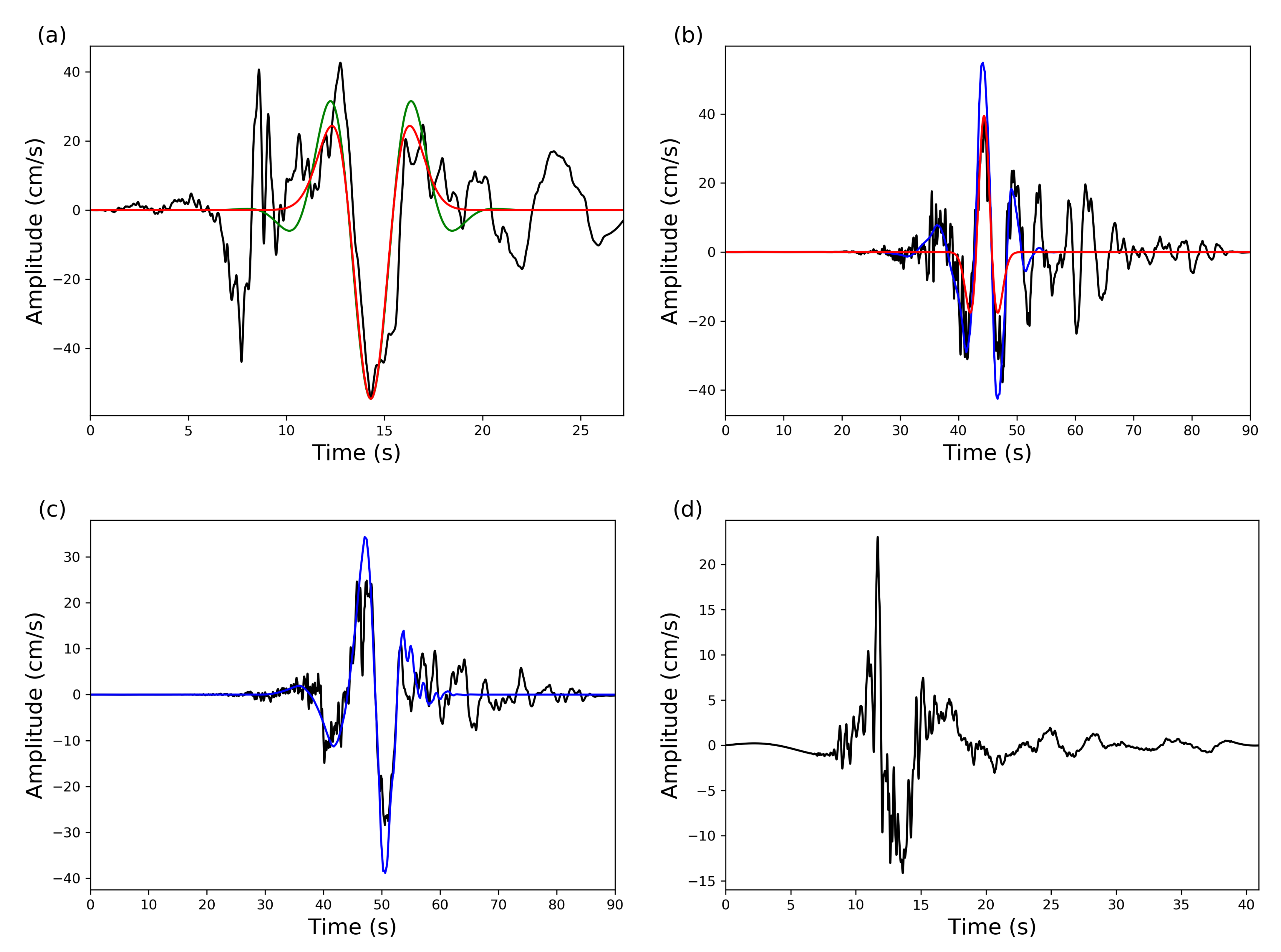
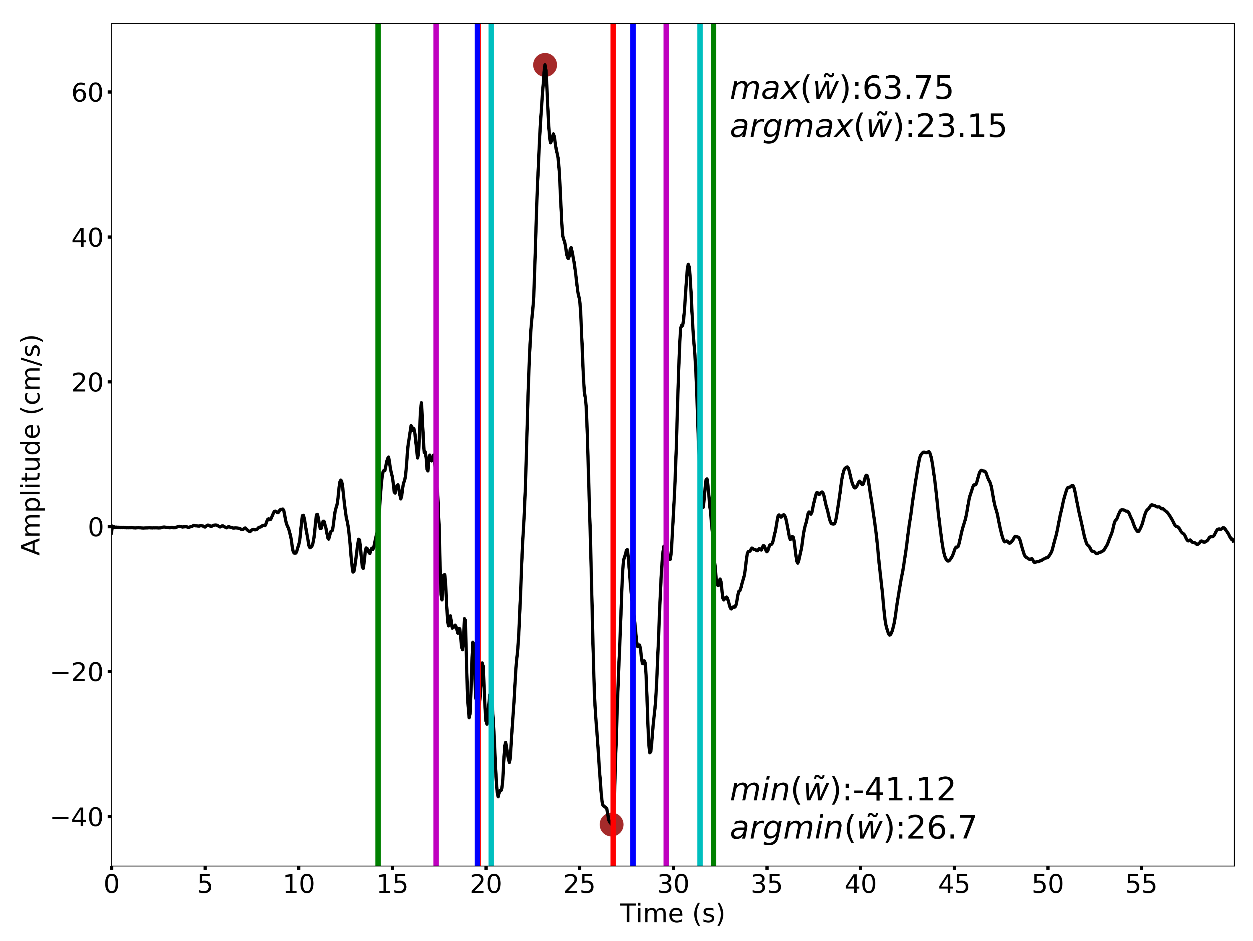
3.2. Determination of Initiation and Termination Positions of Impulsive Signals

The inputs of this neural network are vectors of ${\overrightarrow{w}}^{\prime }$ and $\overrightarrow{v}$. Unlike the model for the identification of impulsive signals, the latter is a vector of four components $\langle \max (\overrightarrow{w}),\min (\overrightarrow{w}),arg\; max(\overrightarrow{w}),arg\; min(\overrightarrow{w})\rangle$ (Figure 3). The output of the neural network is a pair of values, s and e, which represent the initiation and termination positions of the velocity pulse.

The model is structured with two different parts (

Table 2. Description of layers used in the model to identify initiation and termination positions of impulsive part of the signals. For each layer the dimension of the layer output is reported.

Layer Type	Output Shape
Input	1200
Conv1D	$1189\times 64$
MaxPooling1D	$297\times 64$
Conv1D	$292\times 16$
MaxPooling1D	$146\times 32$
Conv1D	$144\times 32$
MaxPooling1D	$48\times 32$
Conv1D	$46\times 64$
MaxPooling1D	$15\times 16$
Dropout	$15\times 16$
Flatten	240
Input	4
Concatenate	244
Dense	40
Dense	30
Dense	30
Activation	1

): the first one is the convolutional part, which process ${\overrightarrow{w}}^{\prime }$ in order to extract the relevant pattern from the normalised waveform. The second part is a fully connected neural network, which takes the features extracted by the convolutional part as input and $\overrightarrow{v}$ and outputs the estimated initiations and termination positions. Features of the model (activation functions, learning rate, loss function, and data splitting) are the same as in the identification of impulsive signals.

4. Results

4.1. Cross-Validation of Identification of Impulsive Signals

In order to experimentally assess the method, a five-fold cross-validation is performed. This procedure is important to verify the generalisation of the model by testing it on new, unseen data. Typically, the cross-validation is performed by dividing the dataset into five subsets and repeating the training five times. For each training phase, four subsets are used, then the performance of the neural network on the remaining unseen subset is evaluated. By doing that, the evaluation of the model is not affected by very lucky (or unlucky) data. This paper has a slightly different approach for which only the negative examples (not impulsive signals) are divided into five folds, while four folds are used for the training, and the remaining is used for the testing. Then, an amount of synthetic examples as large as the training set are added to the training set, and all the real positive examples are added into the testing set. The rationale for this choice is two-fold: first of all, we do not want to test the model on synthetic signals, but we want to asses the proposal on real data. Secondly, we want to have a balanced training set to help the network learn how to differentiate between positives and negatives properly. In addition to cross-validation, the training is repeated on each fold five times to deal with the randomness of weight initialisation. The training has been done on an Intel^® Xeon^® Gold 6140 CPU @ 2.30 GHz with 34 cores and equipped with 196 GB of RAM along with Tesla V100 with 16 GB of RAM GPU. The duration of the training process is in the order of dozens of seconds.

The performance of the model is measured by using FPR and FNR. FPR and FNR are calculated as in Equation (2). These indices are averaged among the $5\times 5$ repetitions, and the averaged results are compared. Obtaining a low FNR means that the method is able to correctly identify the large amount of impulsive signals, whereas a low FPR indicates that the model tends to classify a signal as impulsive only if it is actually impulsive.

$$\begin{array}{cc}\hfill \mathrm{FPR}& =\frac{\mathrm{False}\mathrm{Positive}}{\mathrm{False}\mathrm{Positive}+\mathrm{True}\mathrm{Negative}}\hfill \\ \hfill \mathrm{FNR}& =\frac{\mathrm{False}\mathrm{Negative}}{\mathrm{False}\mathrm{Negative}+\mathrm{True}\mathrm{Positive}}\hfill \end{array}$$

(2)

The performance of the models are compared against three strong baselines Shahi and Baker [17], Chang et al. [22], Ertuncay and Costa [23]. The comparison has been done using the exact same portions of data for all methods during the cross-validation. The results of the comparison have been reported in

Table 3. FRP and FNR averaged over the 5-folds.

Method	Noise	FPR	FNR
Shahi & Baker (2014)		0.003	0.279
Chang et al. (2016)		0.002	0.328
Ertuncay & Costa (2019)		0.043	0.320
Mavroeidis Model	Sabetta and Pugliese [35]	0.206	0.360
Mavroeidis Model	1 std	0.223	0.356
Mavroeidis Model	2 std	0.161	0.381
Mavroeidis Model	3 std	0.187	0.386
$k^{-2}$ Model	Sabetta and Pugliese [35]	0.421	0.062
$k^{-2}$ Model	1 std	0.223	0.356
$k^{-2}$ Model	2 std	0.214	0.446
$k^{-2}$ Model	3 std	0.318	0.378

. Each row shows the performance in terms of FPR and FNR for each method, ours and the baselines. We remark that, because of the disproportion between positive and negative examples, it is important to evaluate both this method and the baselines using two performance indices instead of a single one, such as accuracy, which could be tainted by unbalanced data.

Table 3 shows the performance of previous studies along with the models. It must be taken into account that only synthetic signals are used as positive examples for the training phase. Synthetic signals are enriched by using the method from Sabetta and Pugliese [35] and Gaussian noise with zero mean and 1–3 std. As explained in Section 1, impulsive signals may be created due to many reasons. For instance, in the velocity structure that is used for the synthetic waveforms, weak local soil condition is not implemented. Parameters such as rupture velocity, stress drop, soil conditions [45], and rise time [40] may create impulsive signals. None of these parameters are used as a variable in the synthetics. Limits on the creation of impulsive signals reduce the variation of the pulse shapes of the synthetics.

Both of the models show worse performance with respect to the previous studies in FPR. It means that the models tend to predict a given waveform as impulsive. It can be tolerable up to certain point since the definition of the impulsive motions can vary depending on the decision maker (human interpreter or algorithm). The Mavroeidis model has a smaller FPR with respect to $k^{-2}$ model, however it performs worse than previous algorithms. Even though the $k^{-2}$ model has the worst performance in FPR, it has the best performance in FNR. The FNR of Mavroeidis is in the same level of the previous studies.

4.2. Cross-Validation of Determination of Initiation and Termination Positions of Impulsive Signals

We experimentally assess the model performing a five-fold cross-validation on 534 impulsive signals and compare the results of the CNN with three challenging baselines Shahi and Baker [17], Chang et al. [22], Ertuncay and Costa [23]. Since some of the baselines cannot correctly extract s and e from a given signal, the signals where none of the baseline methods can find the initiation and the termination points are removed from each of the five testing sets. The total number of removed signals are six. This way, all the methods are compared on the same signals. To evaluate the performance of these four methods, ours and the baselines, three performance indices for measuring the errors (see in Section 1) are defined.

Concerning the MSE and MAE, the lower the value, the better the method, whereas $R^2$ ranges between 0 and 1 and a value closer to the maximum indicate a fitter model. In the experimental evaluation, these indices are calculated by averaging them among the five repetitions at the end of the cross-fold procedure. Since the output of the model is a pair of values (s and e), both the error in individuating the right values of s and of e and also the average error in finding both of them ($\mu$) are evaluated. This way, the model is valid independent of the data used to train the neural network. The neural network is trained on the same computers that are explained in Section 4.1. The duration of the training process is in the order of dozens of seconds.

The results of the cross-validation procedure are summarised in

Table 4. Results of all methods averaged among 5-fold cross-validation.

	${\mathit{R}}^2$			MAE			MSE
Method	s	e	$\mathit{\mu }$	s	e	$\mathit{\mu }$	s	e	$\mathit{\mu }$
Chang et al. (2016)	0.95	0.97	0.96	19.60	12.85	21.40	844.41	1171.01	1007.71
CNN	0.97	0.97	0.97	17.51	22.53	20.03	610.23	1057.47	833.85
Ertuncay and Costa (2019)	0.94	0.97	0.95	24.27	25.79	25.03	1190.31	1154.98	1172.65
Shahi and Baker (2014)	0.95	0.98	0.96	22.55	20.56	21.55	978.44	812.89	895.77

. The table reports the averaged values for $R^2$, MAE, and MSE for all the methods measured on the initiation and termination points and the average between them. The comparison shows how the model outperforms the baselines in finding the initiation point of the impulsive waveform: the CNN obtained a better score considering all the different indices. Concerning the termination point, Chang et al. [22] is the best method, but our model is the second-best one. Globally, our method is the best if the MSE index is considered and is even with Chang et al. [22] with respect to $R^2$.

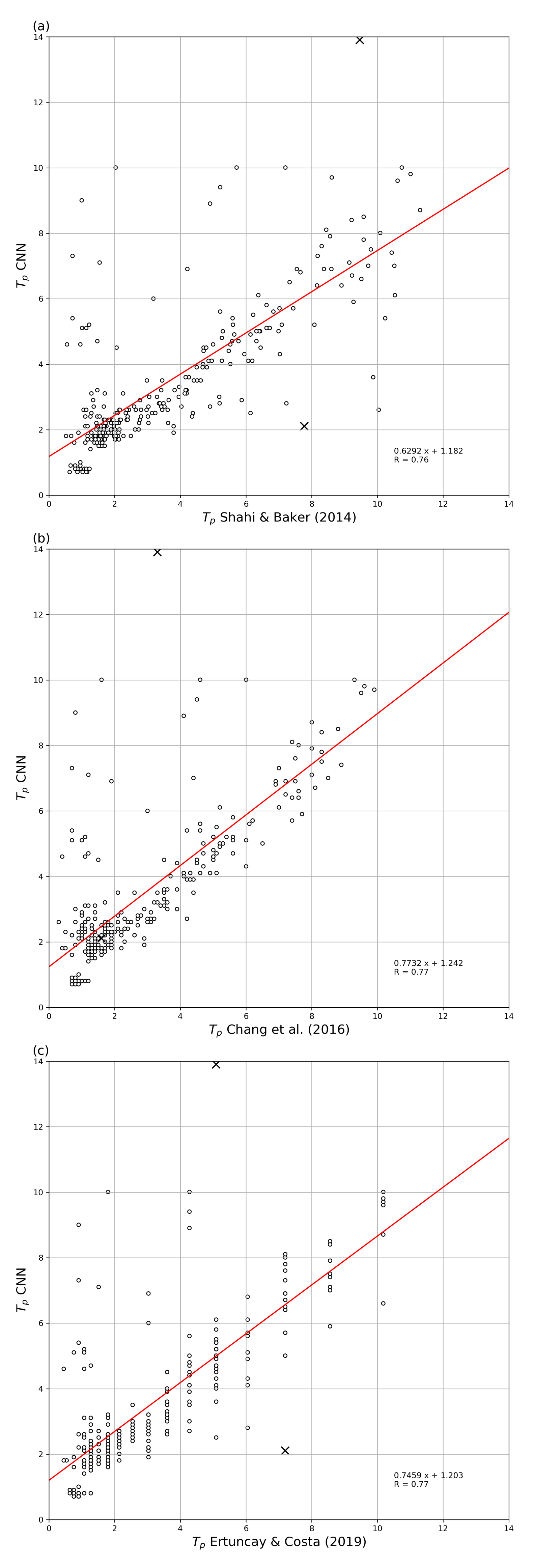
4.3. Comparison of Pulse Periods

The period of the impulsive signal is important due to its destructive effect on the structure (Section 1). After the determination of the initiation and termination points of the impulsive part of the velocity waveform, its period is determined. To do that, the pseudo-spectral velocity of the impulsive part of the signal is calculated. The period of the largest amplitude is assigned as the period of the impulsive signal.

The spectral velocity of the fitted wavelets of the previous studies is calculated to compare with our model. The correlation of $T_p$ between Shahi and Baker [17], Chang et al. [22], Ertuncay and Costa [23], and our model are investigated. Before the investigation, velocity waveforms are smoothed. Smoothing is applied to remove high-frequency signals embedded inside the long-period signal. The high-frequency noise creates larger amplitudes in shorter periods, which leads to very low $T_p$ for the CNN model. The central moving average method has been implemented with a 10 moving average to do the smoothing. Correlation coefficients (R) are around 0.77 for all of them (Figure 4). There are several incidences where the differences between the measured periods are unexpectedly large. These outliers are given with x symbols in Figure 4. The reasons for the difference are discussed case by case.

4.4. Outliers

The first outlier is the El Centro Array #5 station record in 15th of October 1979 Imperial Valley, USA earthquake (Figure 5). The pulse period of the signal is determined as $3.30$ $\mathrm{s}$, $5.09$ $\mathrm{s}$, $9.46$ $\mathrm{s}$, and $13.61$ $\mathrm{s}$ by Chang et al. [22], Ertuncay and Costa [23], Shahi and Baker [17], and the CNN model, respectively. Chang et al. [22] and Ertuncay and Costa [23] are concentrated to the arrival of PGV, whereas Shahi and Baker [17] is concentrated to the general trend of the waveform. Ertuncay and Costa [23] is able to capture the long period in the spectral domain with correct amplitudes. The developed model was able to correctly determine the ending position of the impulsive part of the waveform. However, it failed to locate the starting position, which caused a miscalculated pulse period.

The second outlier is the Lucerne station record in 28th of June 1992 Landers, USA earthquake (Figure 6). The pulse period of the signal is determined as $1.60$ $\mathrm{s}$, $7.19$ $\mathrm{s}$, $7.77$ $\mathrm{s}$, and $1.61$ $\mathrm{s}$ by Chang et al. [22], Ertuncay and Costa [23], Shahi and Baker [17], and the CNN model, respectively. In this case, both Ertuncay and Costa [23] and Shahi and Baker [17] are able to locate long-period (≥ $5.5$ $\mathrm{s}$) information, but none of these studies capture the amplitude information correctly. The model captured the period of the largest amplitude $1.61$ $\mathrm{s}$ similar to Chang et al. [22]. Due to the false prediction of the termination position, the model failed to capture the larger period information properly. Even if the model captured the termination position properly, it would not change the pulse period since the amplitude of $1.61$ $\mathrm{s}$ is larger than the amplitudes at around $5.5$ $\mathrm{s}$. It is important to underline that the pulse period calculation is not done by the CNN model but by a very simple method of measuring the period of the maximum amplitude inside the predicted locations of the impulsive part of the waveform by the model.

It is important to clarify that outliers do not necessarily mean that one method is superior to another. Previous studies used different approaches to explain impulsive parts. In this study, impulsive motions are detected by an expert using visual inspection. Hence, the model learns the features of the impulsive signals and labels the initiation and termination points accordingly. A very simple decision algorithm, which is selecting the period with the largest amplitude both in the determination of the $T_p$ of manual signals and the CNN model, is used. There can be two major periods with large amplitudes in the spectral domain. In such cases, it is better to check the initiation and termination points of the model or fitted wavelets of previous studies to decide about the pulse period.

5. Discussion and Conclusions

In this study, we proposed two CNN models for detecting impulsive velocity waveforms and a model for the position of the impulsive behaviour of a given waveform. To identify the impulsive signals, the neural network using both real and synthetic signals is trained, where the last ones were created in order to equalise the ratio between impulsive and non-impulsive signals. Real impulsive signals are detected manually, and the performance of the CNN method is measured by using these waveforms as ground truth.

Unlike the previous studies, CNN methods make predictions by learning the features of the impulsive signals given in the training phase. Thus, there are no ratios, wave fitting, or thresholds in the model. Instead, it “learns” the features of the impulsive and non-impulsive signals by using a set of activation functions and convolutions.

CNN could help overcome the decision-making problem on impulsive signals even though our models require further investigation to increase the performance. Both Mavroneidis and $k^{-2}$ models perform worse than three robust previous studies that are used as a baseline. $k^{-2}$ has the FNR ratio, but it also has the worst FPR ratio. The Mavroneidis model has more stable results in both metrics, and its FNR is almost as good as the previous studies.

Many reasons may have played a role in the results. As mentioned in the Section 1, impulsive signals can be seen as a result of multiple sources. Neither Mavroneidis nor $k^{-2}$ models can cover all these sources. Mavroeidis and Papageorgiou [20] created a mathematical formula by using the limited amount of impulsive signals. Many impulsive signals are detected after this study, and the mathematical model may require further adjustments to model the later recorded motions. Moreover, synthetics created by this algorithm cannot cover any of these effects. The $k^{-2}$ model requires physics-based inputs to create synthetics. However, this model does not cover effects, such as fling step and local soil conditions.

Furthermore, the study of Sabetta and Pugliese [35] is used for high-frequency content to enrich the synthetics, which does not cover all the effects of a shallow surface. White Gaussian noise with standard deviations from one to three instead of the methodology of Sabetta and Pugliese [35] is also used. Synthetics-added increasing standard deviation tend to label signals as non-impulsive. False positives, on the other hand, have no trend, and the best result is obtained with synthetics added 2 std Gaussian noise. The best model among Mavroeidis models is the one with 2 std noise. In the $k^{-2}$ model, Gaussian noise significantly increases the false negatives whereas decreases the false positives. On average, synthetics enriched with the method of Sabetta and Pugliese [35] have the best performance in terms of the average FPR and FNR. In general, Mavroeidis models have more stable results regardless of the noise type, whereas $k^{-2}$ models vary between Sabetta and Pugliese [35] and Gaussian noises, but $k^{-2}$ models have stable results among Gaussian noises.

The CNN method understood the nature of the impulsive signals by training only on synthetic impulsive velocity waveforms. Lack of the representation of the effects that played role on the creation of ground motions that are identified as impulsive in synthetics signals may reduce the accuracy of the models. CNNs do not need any mathematical formulations or thresholds to make decisions about the impulsiveness of a waveform but instead, depend only on the used training set.

In the second part of the study, initiation and termination positions of the given impulsive motion are determined. Thanks to the modular structure of our study, one can use the models depending on their needs. The second part works independent from the first part; hence, one can use the previous studies to detect impulsive signals and use our initiation and termination model to detect the location of the impulsive motions.

To identify the initiation and the termination positions of a given impulsive signal, we proposed a convolutional neural network fed with the impulsive signal and some ancillary inputs that help the network identify the relevant points. The results were compared with three very challenging baselines on the same data, and the comparison shows how our method is better at identifying the initiation point and is in second place concerning the termination point. Our proposal clearly outperforms all three baselines, although the differences between previous studies and our proposal are not significantly large.

In addition, the determined impulsive periods were compared. In most short period impulsive signals, our model and previous models are in agreement. However, there are several signals in which $T_p$ is determined with large variance among the previous studies and our model. These examples were analysed in detail and found that in the presence of multiple large-amplitude periods, previous models tend to focus on one of them depending on their algorithms. In such cases, it is more logical to determine the initiation and termination of the impulsive part of the waveform and further analyse each waveform. Thus, our model is a good candidate to detect the impulsive parts of the signals. Although our proposal has to be investigated further, we believe that our results are very promising and can be a starting point for further research in this field.

More advanced synthetic ground motion creation algorithms may be used in the future to help cover the multiple aspects of the motions. The effects of permanent displacement of the ground and directivity effect can be investigated in both azimuth and distance. Fault plane information, such as the dip and rake angle, and hypocentral distance, may also be implemented to have variation on impulsive motions. Site conditions, such as the basin effect and shallow soil conditions, may also be modelled to see their effects.

References

1. Baltzopoulos, G.; Luzi, L.; Iervolino, I. Analysis of Near-Source Ground Motion from the 2019 Ridgecrest Earthquake Sequence. Bull. Seismol. Soc. Am. 2020, 110, 1495–1505. [Google Scholar] [CrossRef]
2. Somerville, P.G.; Smith, N.F.; Graves, R.W.; Abrahamson, N.A. Modification of empirical strong ground motion attenuation relations to include the amplitude and duration effects of rupture directivity. Seismol. Res. Lett. 1997, 68, 199–222. [Google Scholar] [CrossRef]
3. Kalkan, E.; Adalier, K.; Pamuk, A. Near source effects and engineering implications of recent earthquakes in Turkey. In International Conference on Case Histories in Geotechnical Engineering; University of Missouri–Rolla: Rolla, MO, USA, 2004; Volume 19. [Google Scholar]
4. Kobayashi, H.; Koketsu, K.; Miyake, H. Rupture processes of the 2016 Kumamoto earthquake sequence: Causes for extreme ground motions. Geophys. Res. Lett. 2017, 44, 6002–6010. [Google Scholar] [CrossRef]
5. Asano, K.; Iwata, T. Source rupture process of the 2018 Hokkaido Eastern Iburi earthquake deduced from strong-motion data considering seismic wave propagation in three-dimensional velocity structure. Earth Planets Space 2019, 71, 101. [Google Scholar] [CrossRef]
6. Kobayashi, H.; Koketsu, K.; Miyake, H. Rupture process of the 2018 Hokkaido Eastern Iburi earthquake derived from strong motion and geodetic data. Earth Planets Space 2019, 71, 63. [Google Scholar] [CrossRef]
7. Kalkan, E.; Kunnath, S.K. Effects of fling step and forward directivity on seismic response of buildings. Earthq. Spectra 2006, 22, 367–390. [Google Scholar] [CrossRef]
8. Bradley, B.A. Strong ground motion characteristics observed in the 4 September 2010 Darfield, New Zealand earthquake. Soil Dyn. Earthq. Eng. 2012, 42, 32–46. [Google Scholar] [CrossRef]
9. Shahi, S.K.; Baker, J.W. An empirically calibrated framework for including the effects of near-fault directivity in probabilistic seismic hazard analysis. Bull. Seismol. Soc. Am. 2011, 101, 742–755. [Google Scholar] [CrossRef]
10. Iervolino, I.; Chioccarelli, E.; Baltzopoulos, G. Inelastic displacement ratio of near-source pulse-like ground motions. Earthq. Eng. Struct. Dyn. 2012, 41, 2351–2357. [Google Scholar] [CrossRef]
11. Iervolino, I.; Baltzopoulos, G.; Chioccarelli, E.; Suzuki, A. Seismic actions on structures in the near-source region of the 2016 central Italy sequence. Bull. Earthq. Eng. 2017, 17, 5429–5447. [Google Scholar] [CrossRef]
12. Li, C.; Kunnath, S.; Zuo, Z.; Peng, W.; Zhai, C. Effects of early-arriving pulse-like ground motions on seismic demands in RC frame structures. Soil Dyn. Earthq. Eng. 2020, 130, 105997. [Google Scholar] [CrossRef]
13. Guo, G.; Yang, D.; Liu, Y. Duration effect of near-fault pulse-like ground motions and identification of most suitable duration measure. Bull. Earthq. Eng. 2018, 16, 5095–5119. [Google Scholar] [CrossRef]
14. Mazza, F. Seismic demand of base-isolated irregular structures subjected to pulse-type earthquakes. Soil Dyn. Earthq. Eng. 2018, 108, 111–129. [Google Scholar] [CrossRef]
15. Antonellis, G.; Panagiotou, M. Seismic response of bridges with rocking foundations compared to fixed-base bridges at a near-fault site. J. Bridge Eng. 2013, 19, 04014007. [Google Scholar] [CrossRef]
16. Iervolino, I.; Cornell, C.A. Probability of occurrence of velocity pulses in near-source ground motions. Bull. Seismol. Soc. Am. 2008, 98, 2262–2277. [Google Scholar] [CrossRef]
17. Shahi, S.K.; Baker, J.W. An efficient algorithm to identify strong-velocity pulses in multicomponent ground motions. Bull. Seismol. Soc. Am. 2014, 104, 2456–2466. [Google Scholar] [CrossRef]
18. Ertuncay, D.; Costa, G. Determination of near-fault impulsive signals with multivariate naïve Bayes method. Nat. Hazards 2021, 108, 1763–1780. [Google Scholar] [CrossRef]
19. Chioccarelli, E.; Iervolino, I. Near-source seismic hazard and design scenarios. Earthq. Eng. Struct. Dyn. 2013, 42, 603–622. [Google Scholar] [CrossRef]
20. Mavroeidis, G.P.; Papageorgiou, A.S. A mathematical representation of near-fault ground motions. Bull. Seismol. Soc. Am. 2003, 93, 1099–1131. [Google Scholar] [CrossRef]
21. Baker, J.W. Quantitative classification of near-fault ground motions using wavelet analysis. Bull. Seismol. Soc. Am. 2007, 97, 1486–1501. [Google Scholar] [CrossRef]
22. Chang, Z.; Sun, X.; Zhai, C.; Zhao, J.X.; Xie, L. An improved energy-based approach for selecting pulse-like ground motions. Earthq. Eng. Struct. Dyn. 2016, 45, 2405–2411. [Google Scholar] [CrossRef]
23. Ertuncay, D.; Costa, G. An alternative pulse classification algorithm based on multiple wavelet analysis. J. Seismol. 2019, 23, 929–942. [Google Scholar] [CrossRef] [Green Version]
24. Mousavi, S.M.; Sheng, Y.; Zhu, W.; Beroza, G.C. STanford EArthquake Dataset (STEAD): A Global Data Set of Seismic Signals for AI. IEEE Access 2019, 7, 179464–179476. [Google Scholar] [CrossRef]
25. Meier, M.A.; Ross, Z.E.; Ramachandran, A.; Balakrishna, A.; Nair, S.; Kundzicz, P.; Li, Z.; Andrews, J.; Hauksson, E.; Yue, Y. Reliable real-time seismic signal/noise discrimination with machine learning. J. Geophys. Res. Solid Earth 2019, 124, 788–800. [Google Scholar] [CrossRef] [Green Version]
26. Mousavi, S.M.; Ellsworth, W.L.; Zhu, W.; Chuang, L.Y.; Beroza, G.C. Earthquake transformer—An attentive deep-learning model for simultaneous earthquake detection and phase picking. Nat. Commun. 2020, 11, 1–12. [Google Scholar] [CrossRef] [PubMed]
27. Ross, Z.E.; Meier, M.A.; Hauksson, E. P wave arrival picking and first-motion polarity determination with deep learning. J. Geophys. Res. Solid Earth 2018, 123, 5120–5129. [Google Scholar] [CrossRef]
28. Ross, Z.E.; Meier, M.A.; Hauksson, E.; Heaton, T.H. Generalized seismic phase detection with deep learning. Bull. Seismol. Soc. Am. 2018, 108, 2894–2901. [Google Scholar] [CrossRef] [Green Version]
29. Titos, M.; Bueno, A.; García, L.; Benítez, M.C.; Ibañez, J. Detection and Classification of Continuous Volcano-Seismic Signals with Recurrent Neural Networks. IEEE Trans. Geosci. Remote Sens. 2018, 57, 1936–1948. [Google Scholar] [CrossRef]
30. Titos, M.; Bueno, A.; García, L.; Benítez, C. A Deep Neural Networks Approach to Automatic Recognition Systems for Volcano-Seismic Events. IEEE J. Sel. Top. Appl. Earth Obs. Remote Sens. 2018, 11, 1533–1544. [Google Scholar] [CrossRef]
31. Mousavi, S.M.; Beroza, G.C. A machine-learning approach for earthquake magnitude estimation. Geophys. Res. Lett. 2020, 47, e2019GL085976. [Google Scholar] [CrossRef] [Green Version]
32. Somerville, P.G. Magnitude scaling of the near fault rupture directivity pulse. Phys. Earth Planet. Inter. 2003, 137, 201–212. [Google Scholar] [CrossRef]
33. Bozorgnia, Y.; Abrahamson, N.A.; Atik, L.A.; Ancheta, T.D.; Atkinson, G.M.; Baker, J.W.; Baltay, A.; Boore, D.M.; Campbell, K.W.; Chiou, B.S.J.; et al. NGA-West2 research project. Earthq. Spectra 2014, 30, 973–987. [Google Scholar] [CrossRef] [Green Version]
34. Boore, D.M.; Watson-Lamprey, J.; Abrahamson, N.A. Orientation-independent measures of ground motion. Bull. Seismol. Soc. Am. 2006, 96, 1502–1511. [Google Scholar] [CrossRef]
35. Sabetta, F.; Pugliese, A. Estimation of response spectra and simulation of nonstationary earthquake ground motions. Bull. Seismol. Soc. Am. 1996, 86, 337–352. [Google Scholar]
36. Causse, M.; Chaljub, E.; Cotton, F.; Cornou, C.; Bard, P.Y. New approach for coupling k- 2 and empirical Green’s functions: Application to the blind prediction of broad-band ground motion in the Grenoble basin. Geophys. J. Int. 2009, 179, 1627–1644. [Google Scholar] [CrossRef] [Green Version]
37. Bernard, P.; Herrero, A.; Berge, C. Modeling directivity of heterogeneous earthquake ruptures. Bull. Seismol. Soc. Am. 1996, 86, 1149–1160. [Google Scholar]
38. Ameri, G.; Gallovič, F.; Pacor, F. Complexity of the Mw 6.3 2009 L’Aquila (central Italy) earthquake: 2. Broadband strong motion modeling. J. Geophys. Res. Solid Earth 2012, 117. [Google Scholar] [CrossRef] [Green Version]
39. Coutant, O. Programme de Simulation Numerique AXITRA. Rapport LGIT, Granoble. 1989. Available online: https://github.com/coutanto/axitra (accessed on 20 July 2021).
40. Scala, A.; Festa, G.; Del Gaudio, S. Relation Between Near-Fault Ground Motion Impulsive Signals and Source Parameters. J. Geophys. Res. Solid Earth 2018, 123, 7707–7721. [Google Scholar] [CrossRef]
41. Abadi, M.; Barham, P.; Chen, J.; Chen, Z.; Davis, A.; Dean, J.; Devin, M.; Ghemawat, S.; Irving, G.; Isard, M.; et al. Tensorflow: A system for large-scale machine learning. In Proceedings of the 12th USENIX Symposium on Operating Systems Design and Implementation (OSDI 16), Savannah, GA, USA, 2–4 November 2016; pp. 265–283. [Google Scholar]
42. Chollet, F. Keras. 2015. Available online: https://keras.io (accessed on 25 July 2021).
43. Kingma, D.P.; Ba, J. Adam: A method for stochastic optimization. arXiv 2014, arXiv:1412.6980. [Google Scholar]
44. Glorot, X.; Bengio, Y. Understanding the difficulty of training deep feedforward neural networks. In Proceedings of the Thirteenth International Conference on Artificial Intelligence and Statistics, Sardinia, Italy, 13–15 May 2010; pp. 249–256. [Google Scholar]
45. Cork, T.G.; Kim, J.H.; Mavroeidis, G.P.; Kim, J.K.; Halldorsson, B.; Papageorgiou, A.S. Effects of tectonic regime and soil conditions on the pulse period of near-fault ground motions. Soil Dyn. Earthq. Eng. 2016, 80, 102–118. [Google Scholar] [CrossRef]
46. Aristotle University of Thessaloniki Seismological Network. Permanent Regional Seismological Network Operated by the Aristotle University of Thessaloniki. 1981. Available online: http://geophysics.geo.auth.gr/the_seisnet/WEBSITE_2005/station_index_en.html (accessed on 11 September 2021). [CrossRef]
47. Boğaziçi University Kandilli Observatory and Earthquake Research Institute. 2001. Available online: http://www.koeri.boun.edu.tr/sismo/2/en/ (accessed on 11 September 2021). [CrossRef]
48. Institute of Earth Sciences, Academia Sinica. Broadband Array in Taiwan for Seismology; Institute of Earth Sciences, Academia Sinica: Taipei, Taiwan, 1996. [Google Scholar]
49. Geological Survey of Canada. Canadian National Seismograph Network; Geological Survey of Canada: Ottawa, ON, USA, 1989. [Google Scholar] [CrossRef]
50. AFAD. AFAD—Turkey Earthquake Data Center System. 2019. Available online: https://tadas.afad.gov.tr/ (accessed on 11 September 2021).
51. Van Houtte, C.; Bannister, S.; Holden, C.; Bourguignon, S.; McVerry, G. The New Zealand strong motion database. Bull. New Zeal. Soc. Earthq. Eng. 2017, 50, 1–20. [Google Scholar] [CrossRef]
52. National Observatory of Athens. National Observatory of Athens Seismic Network; National Observatory of Athens: Athina, Greece, 1997. [Google Scholar] [CrossRef]
53. Institute of Engineering Seimology Earthquake Engineering. ITSAK Strong Motion Network; Institute of Engineering Seimology Earthquake Engineering: Thessaloniki, Greece, 1981. [Google Scholar] [CrossRef]
54. Earth Science and Resilience. NIED K-NET, KiK-net. 2019. Available online: https://www.kyoshin.bosai.go.jp/ (accessed on 11 September 2021).
55. SSN. Servicio Sismologico Nacional. 2017. Available online: http://www.ssn.unam.mx/ (accessed on 11 September 2021). [CrossRef]
56. Universidad De Chile. Red Sismologica Nacional; University of Chile: Metropolitana, Chile, 2013. [Google Scholar] [CrossRef]
57. Technological Educational Institute of Crete. Seismological Network of Crete; Technological Educational Institute of Crete: Iraklio, Greece, 2006. [Google Scholar] [CrossRef]
58. GEOFON Data Centre. GEOFON Seismic Network; GEOFON Data Centre: Potsdam, Germany, 1993. [Google Scholar] [CrossRef]
59. Luzi, L.; Puglia, R.; Russo, E.; D’Amico, M.; Felicetta, C.; Pacor, F.; Lanzano, G.; Çeken, U.; Clinton, J.; Costa, G.; et al. The engineering strong-motion database: A platform to access pan-European accelerometric data. Seismol. Res. Lett. 2016, 87, 987–997. [Google Scholar] [CrossRef] [Green Version]
60. Pacor, F.; Paolucci, R.; Luzi, L.; Sabetta, F.; Spinelli, A.; Gorini, A.; Nicoletti, M.; Marcucci, S.; Filippi, L.; Dolce, M. Overview of the Italian strong motion database ITACA 1.0. Bull. Earthq. Eng. 2011, 9, 1723–1739. [Google Scholar] [CrossRef] [Green Version]
Figure 1. (a) The distribution of earthquakes (red stars) and stations (blue dots); (b) a histogram of the number of manually detected impulsive (orange) and non-impulsive (blue) signals with M w with a 0.1 interval; (c) a histogram of the number of impulsive and non-impulsive signals with epicentral distance with a 10 k m interval.
Geosciences 11 00388 g001
Figure 2. (a) Velocity waveform (black) of the radial component of Düzce station ( R j b =   13.6   k m ) in the 17th of August 1999 Kocaeli, Turkey earthquake ( M w = 7.5); (b) velocity waveform of the radial component of TCU038 station ( R j b =   25.4   k m ) in the 20th of September 1999 Chi-Chi, Taiwan, earthquake ( M w = 7.6); (c) velocity waveform of the transverse component of TCU026 station ( R j b =   56.0   k m ) in the Chi-Chi, Taiwan earthquake; (d) velocity waveform of the radial component of 4809 station ( R j b =   7.8   k m ) in the 21st of July 2017 Aegean Sea earthquake ( M w = 6.5). Green, red, and blue wavelets are fitted wavelets determined by Shahi and Baker [9], Chang et al. [22], Ertuncay and Costa [23], respectively.
Geosciences 11 00388 g002
Figure 3. Representation of the waveform ( w ) and the input data ( v ) on the 23rd of November 1980 Irpinia, Italy earthquake ( M w = 6.9) ground motion record at Arienzo station ( R j b = 52.93   k m ). Initiation and termination positions of manual picking, CNN model, Chang et al. [22], Ertuncay and Costa [23], and Shahi and Baker [17] are given with cyan, magenta, green, red, and blue colours, respectively.
Geosciences 11 00388 g003
Figure 4. Comparison between pulse periods found by (a) Shahi and Baker [17], (b) Chang et al. [22], and (c) Ertuncay and Costa [23]. Red lines are the regression lines, and their formulate with R value are given on lower left. Outliers are plotted with x, and other impulsive signals are plotted with ◯.
Geosciences 11 00388 g004
Figure 5. (a) Spectral response and (b) velocity waveform of the 15th of October 1979 Imperial Valley, USA earthquake ( M w  = 6.5) recorded at El Centro Array #5 station ( R j b  =  29.5   k m ) along with fitted waveforms and their spectral responses of previous studies. Colour and T p information are the same as in Figure 3.
Geosciences 11 00388 g005
Figure 6. (a) Spectral response and (b) velocity waveform of the 28th of June 1992 Landers, USA earthquake ( M w  = 7.3) recorded at Lucerne station ( R j b  =  2.2   k m ) along with fitted waveforms and their spectral responses of previous studies. Color and T p information are the same as in Figure 3.
Geosciences 11 00388 g006