Analysis of the Northern Hemisphere Atmospheric Circulation Response to Arctic Ice Reduction Based on Simulation Results

Abstract

The amplified warming of the Arctic is one of several factors influencing atmospheric dynamics. In this work, we consider a series of numerical experiments to identify the role of Arctic sea ice reduction in affecting climate trends in the Northern Hemisphere. With this aim in mind, we use two independent mechanisms of ice reduction. The first is traditionally associated with increasing the concentration of carbon dioxide in the atmosphere from the historic level of 360 ppm to 450 ppm and 600 ppm. This growth increases air temperature and decreases the ice volume. The second mechanism is associated with a reduction in the reflectivity of ice and snow. We assume that comparing the results of these two experiments allows us to judge the direct role of ice reduction. The most prominent consequences of ice reduction, as a result, are the weakening of temperature gradient at the tropopause level in mid-latitudes; the slower zonal wind at 50–60° N; intensification of wave activity in Europe, Western America, and Chukotka; and its weakening in the south of Siberia and Kazakhstan. We also consider how climate change may alter regimes such as blocking and stationary Rossby waves. The study used the INM-CM48 climate system model.

1. Introduction

Since the mid-20th century, the Arctic is experiencing an entire shift in its ecosystem and environment with many significant impacts [1] including those associated with climate change: warming faster than average global warming and reducing winter and summer sea ice cover. However, the effect of melting sea ice in the Arctic on the global climate remains a matter of debate, particularly its impact on the Atlantic meridional overturning circulation (AMOC).

The response of large-scale atmospheric circulation in winter, which is formed as a result of the boreal summer–fall reduction in the area of floating ice, is characterized by an increase in the meridional component of flows in the atmosphere [2], reminiscent of the negative phase of the Arctic Oscillation (AO), which maintains cold winters in northern Eurasia [3]. Rossby waves with anomalously large amplitudes penetrate the stratosphere in boreal winter and weaken the stratospheric polar vortex [4,5,6,7], generating negative AO anomalies [8,9]. Therefore, one of the motivations for understanding the atmospheric response to the shrinking sea ice in the Arctic is a possible link to extreme weather events in the mid-latitudes. In addition, freshening of the subpolar Arctic due to sea ice melting reduces the intensity of AMOC [10] and associated heat transfer by ocean currents to the north [11], causing heat accumulation in tropical latitudes [12]. The resulting increase in ocean surface temperature in the tropics enhances deep atmospheric convection, and associated latent heat release [13], leading to warming in the tropical upper troposphere.

Currently, there are still gaps in understanding the mechanisms linking Arctic warming, sea ice reduction, stratospheric–tropospheric interactions, and extreme weather events [14]. The relationship between ice reduction and the corresponding changes in the structure of atmospheric circulation, established statistically or using numerical modeling, may not be a relationship between cause and effect. It could be a relationship between two effects of some common cause like atmospheric warming [15].

In the Arctic, the ice–albedo feedback mechanism plays a key role in the balance of heat and ice mass at the ocean surface [16,17]. During the melting season, the sea ice changes its physical condition and optical properties. As the incident solar radiation increases and the air heats up, the ice sheet transforms from a highly diffuse snow-covered medium to a darker mix of bare ice and melt-ponds. Otherwise, the rate of summer thawing and the length of the thawing season are strongly influenced by albedo, which decreases as the melting season progresses. These changes decrease the surface albedo, resulting in greater absorption of solar energy, which increases surface warming and causes additional ice melting, known as sea ice–albedo feedback.

In this work, a series of numerical experiments is considered to identify the direct role of the sea ice reduction process in forming climatic trends in the northern hemisphere. We will use two near-independent mechanisms for reducing ice in our numerical simulations. The first is traditionally associated with an increase in the concentration of carbon dioxide in the atmosphere above the historic level of 360 ppm. As a result of this increase, the average air temperature in the Arctic grows, and, by this, the volume of ice decreases. However, in this case, it is difficult to identify trends explicitly associated with ice reduction since the consequences arising from an increase in CO₂ and warming of the atmosphere can be more significant and obscure the role of ice reduction. The second experiment is associated with a decrease in the reflectivity of ice and snow—the amount of solar radiation absorbed by the ice increases, and its volume decreases. Under the conditions of this experiment, the change in the atmosphere’s temperature will be a consequence of two competing processes: the atmosphere receives less reflected radiation but more long-wave radiation due to the higher surface temperature. Nevertheless, this approach has a shortage of underestimation in winter ice reduction [18]. When this article was almost ready, we found the recently published paper in [19], which used a similar approach of ice-albedo decrease to analyze the consequences of Arctic ice reduction. Both mechanisms, increase in CO₂ and ice-albedo decrease, are energy conserving according to the authors of [18]. We assume that comparing the results of these experiments with different mechanisms of ice reduction will make it possible to judge the direct role of ice reduction regardless of the reasons that caused this reduction. First, we will consider the sensitivity of atmospheric blocking and wave activity in mid-latitudes to Arctic ice variations.

Jet stream meanders are one of the main causes of weather variability and extreme events in the mid-latitudes. Large amplitudes of the meanders of the jet can cause extreme weather conditions. One way to quantify the jet stream meandering is to calculate the local wave activity (LWA) of finite-amplitude as an amount of the displacement of the contour of the quasi-geostrophic potential vorticity [20]. LWA tends to be negatively correlated with zonal wind, and knowledge of regions of its high values helps identify the localization of blocking events. Winds in the Earth’s middle latitudes are directed mainly to the east, and their speed increases with height, forming a jet stream in the middle and upper troposphere. The jet stream carries cyclones and anticyclones, which in turn cause meandering of the jet stream. This wave structure also moves eastward, forming unsteady Rossby waves. Occasionally, however, the jet stream forms stable meanders in a specific area, disrupting the passage of non-stationary waves—a condition known as blocking.

Blockings are large-scale, quasi-stationary high-pressure anomalous systems (anticyclonic) that sometimes last for several weeks and block or deflect mid-latitude westerly winds [21,22,23,24]. Because of their duration and size, depending on the season and region, blocking events can trigger or contribute to various types of extreme events such as heatwaves, coldwaves, droughts, and episodes of heavy rainfall (see, e.g., in [25] and references therein). The contours of geopotential height 500 hPa and the wind speed determine the jet stream position, and its noticeable deviation to the pole in the corresponding regions indicates blocking. In winter, in northern latitudes, blocking often occurs when a pre-existing quasi-stationary ridge becomes stronger and prevents the motion of non-stationary waves. While this suggests a role for stationary waves in blocking formation [26], the onset of blocking is still poorly understood and remains a complex issue in numerical weather prediction and climate model experiments [27,28]. The previously proposed mechanisms for the formation and maintenance of blockings include the action of unsteady vortices and the internal instability of low-frequency dynamics [29,30,31,32,33]. However, there is no definitive theory for the criterion for the occurrence of blocking. Furthermore, due to an incomplete understanding of the mechanisms, even the definition of blocking remains somewhat subjective [34,35].

2. Methods

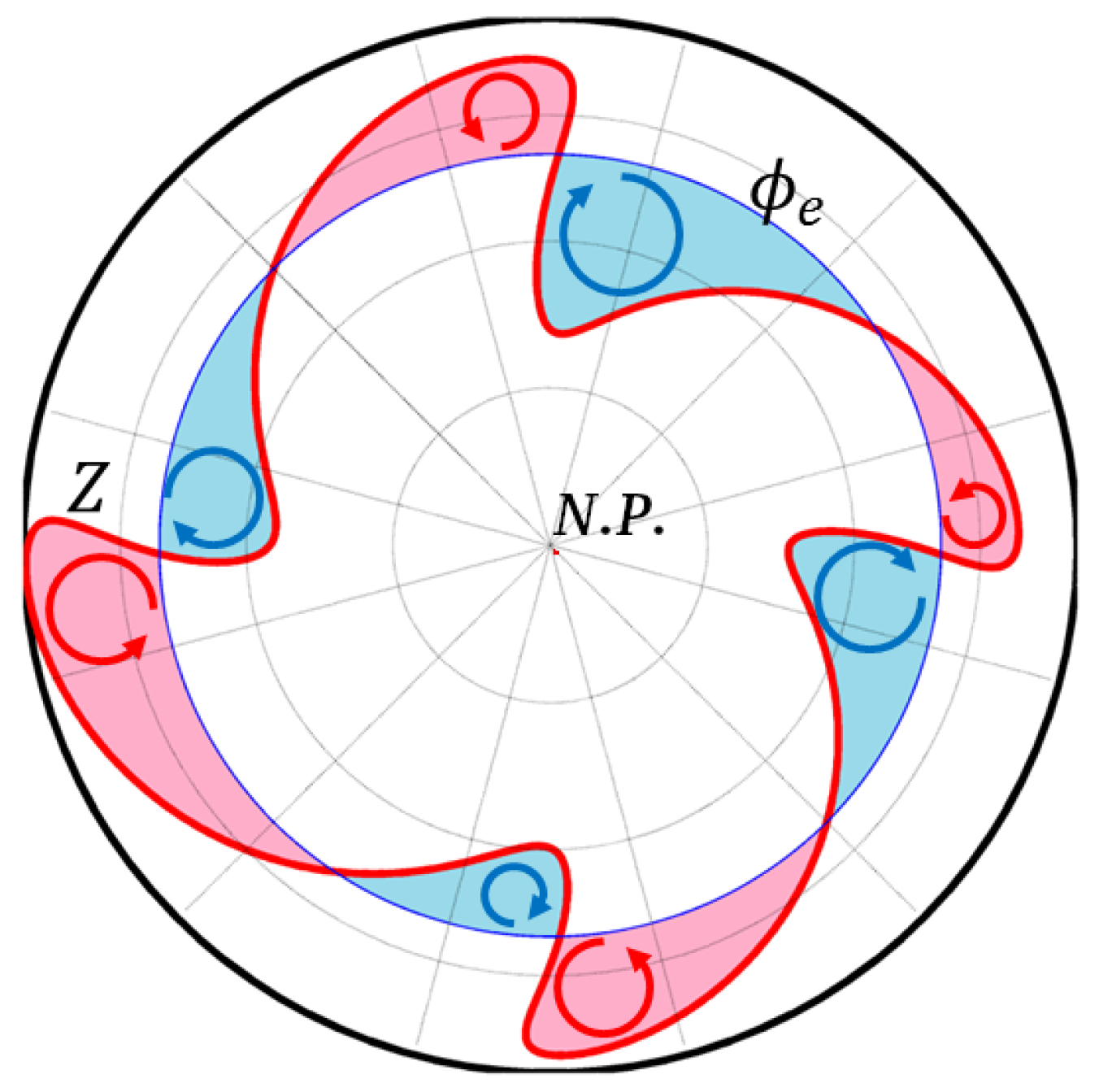
2.1. Local Wave Activity

The best diagnostics for the interaction of vortices and mean flow is wave activity, a measure of the momentum carried by vortices [36]. Wave activity of finite-amplitude was proposed as an objective measure for the spatial variation of a physical quantity, demonstrating monotonicity in the spatial distribution. Finite-amplitude wave activity (FAWA) [37,38,39] is a generalization of the linear wave activity of small amplitude waves.

FAWA (denoted as $A^{*}$) is defined as the area formed when the quasi-geostrophic potential vorticity (QGPV) contour q is displaced from its zonally symmetric state [38]:

$$A^{*}\left({\varphi }_e,z,t\right)=\frac{1}{2\pi acos{\varphi }_e}\left[\underset{\begin{array}{c}q\ge Q\left({\varphi }_e,z,t\right)\\ \frac{\pi }{2}\ge \varphi \end{array}}{\int \int }qdS-\underset{\frac{\pi }{2}\ge \varphi \ge {\varphi }_e}{\int \int }qdS\right],$$

(1)

where ${\varphi }_e$ is the equivalent latitude [40], defined so that the area in both integrals of the following equation would be the same, i.e., equal to Earth’s area higher than ${\varphi }_e$:

$$\underset{\begin{array}{c}q\ge Q\left({\varphi }_e,z,t\right)\\ \frac{\pi }{2}\ge \varphi \end{array}}{\int \int }dS=\underset{\frac{\pi }{2}\ge \varphi \ge {\varphi }_e}{\int \int }dS=2\pi a^2\left(1-sin{\varphi }_e\right),$$

(2)

where $z=-H·log\left(p/1000\right)$, and p is air pressure in hPa, $H$ = 7 km is vertical scale, t is time, $a$ = 6378 km is Earth’s radius, q is QGPV defined as

$$q=f+\zeta +\frac{f}{{\rho }_0}\frac{\partial \left[{\rho }_0\left(\theta -\tilde{\theta }\right)\frac{\partial \tilde{\theta }}{\partial z}\right]}{\partial z},$$

(3)

f is Coriolis parameter, $\theta$ is potential temperature, $\tilde{\theta }$ is zonally averaged potential temperature, ${\rho }_0$ is reference air density, $Q\left({\varphi }_e,z,t\right)$ is Lagrangian mean of QGPV relative to the equivalent latitude ${\varphi }_e$ at each z surface, and $dS=a^{2}cos\varphi d\lambda d\varphi$, where $\lambda$ is longitude.

Equation (1) is also applicable to vortices of arbitrary amplitude as the high limit of low-amplitude waves, similar to the expression for linear waves [37].

Local wave activity (LWA) is a natural generalization of finite-amplitude wave activity regarding a specific range of longitudes. The precise definition of wave activity for potential vorticity and associated dynamic properties is detailed in [37,38]. Recently, Huang and Nakamura [20,41] developed their variant of local wave activity and its associated balance for local wave phenomena such as wave breaking and blocking. Chen et al. [42] further extended the LWA concept to a less conserved value (viz. geopotential height of 500 hPa, designated as $z_{500}$) to facilitate its application. In our study, we also adopt this approach. In particular, for $z_{500}$, which generally has a monotonic distribution in latitude, one can choose the value of its contour Z in the northern hemisphere so that the area S bounded by this Z contour and enclosing the North Pole will be

$$S\left(Z\right)=\underset{z_{500}\le Z}{\int \int }{a}^{2}cos\varphi d\lambda d\varphi .$$

(4)

We can determine the corresponding equivalent latitude ${\varphi }_e$ surrounding the same area in the northern hemisphere. The following formula can establish a one-to-one relationship between ${\varphi }_e$ and the Z value:

$${\varphi }_e=arcsin\left[1-\frac{S\left(Z\right)}{2\pi a^2}\right].$$

(5)

We can introduce two components of LWA corresponding to ${\varphi }_e$ and for each $\lambda$ according to

$$\begin{array}{c}{A}_S\left(\lambda ,{\varphi }_e\right)=\frac{a}{cos{\varphi }_e}\underset{\begin{array}{c}{z}_{500}\le Z\\ \varphi \le {\varphi }_e\end{array}}{\int }\left(z_{500}-Z\right)cos\varphi d\varphi ,\\ A_N\left(\lambda ,{\varphi }_e\right)=\frac{a}{cos{\varphi }_e}\underset{\begin{array}{c}{z}_{500}\ge Z\\ \varphi \ge {\varphi }_e\end{array}}{\int }\left(z_{500}-Z\right)cos\varphi d\varphi .\end{array}$$

(6)

Both components $A_N$ and $-A_S$, determined by (6), are positive definite (Figure 1). The former describes the activity of anticyclonic waves north of the equivalent latitude ${\varphi }_e$, and the latter describes the activity of cyclonic waves south of ${\varphi }_e$. Large and long-lasting $A_N$ values are often associated with atmospheric blocking. The sum of $A_N$ and $-A_S$ gives the total wave activity $A\left({\varphi }_e\right)=A_N-A_S$, a function of ${\varphi }_e$ only. Thus, we return to the original meaning of wave activity as a quantity measuring the total waviness of the Z contour. A simple dimensional analysis shows that we can estimate the overall wave activity as $A\sim \frac{1}{2}{l}^2\frac{d{z}_{500}}{dy}$. Thus, the wave activity can be considered as a result of the displacement of the $z_{500}$ tracer by the meridional disturbance of scale l. The background gradient of this tracer is $\frac{d{z}_{500}}{dy}$. For a typical value of the gradient $\frac{d{z}_{500}}{d{\varphi }_e}$ equal to 8 meters per degree of latitude and a meridional displacement of $\delta \varphi \sim 15°$, the wave activity will be $A\sim {10}^8$ m² [43].

2.2. Blocking Event Index

The interaction of the mean flow and vortices, which leads to the anomalous state of the mid-latitude jet, is associated with propagating and breaking waves in the upper troposphere and stratosphere. Extreme weather events in extratropical latitudes are usually associated with blocking anticyclones. We used the blocking diagnostics proposed by Tibaldi and Molteni (TM) in [44] and further developed in [45], which was used in [46] to obtain the main blocking areas for NCEP/NCAR reanalysis data. They proposed to use the southern and northern gradients of the geopotential height (GHGS and GHGN). For each point with coordinates $\lambda$ and $\varphi$, two indices could be determined as follows:

$$\begin{array}{c}\mathrm{GHGS}(\lambda ,\varphi )=\frac{z_{500}(\lambda ,\varphi )-z_{500}(\lambda ,{\varphi }_S)}{\varphi -{\varphi }_S},\\ \mathrm{GHGN}(\lambda ,\varphi )=\frac{z_{500}(\lambda ,{\varphi }_N)-z_{500}(\lambda ,\varphi )}{{\varphi }_N-\varphi },\end{array}$$

(7)

where ${\varphi }_S=\varphi -15°$, ${\varphi }_N=\varphi +15°$, and $\varphi$ is central latitude of blocking and ranges from 15° N to 75° N. We consider a situation as instant blocking when

$$\begin{array}{c}\mathrm{GHGS}(\lambda ,\varphi )>0,\\ \mathrm{GHGN}(\lambda ,\varphi )<G_n,\end{array}$$

(8)

where $G_n$ is taken to be equal to −5 m·(degree of latitude)${}^{-1}$, although originally in [46] it was −10 m·(degree of latitude)${}^{-1}$. In [47], a modified version of the TM index is used to diagnose and compare blockings in 15 models within the Atmospheric Model Intercomparison Project (AMIP), where it is required that $G_n=-5$ m·(degree of latitude)${}^{-1}$. The reasons for this were related to the improved definition of the Pacific blocking. In this work, two main sectors of the Northern Hemisphere are distinguished, which from the point of view of observations are most susceptible to blocking, that is, the Euro-Atlantic and the Pacific, with the following longitudinal intervals: 26° W–41° E and 115° E–215° W, correspondingly. The criterion $G_n=-10$ m·(degree of latitude)${}^{-1}$ or less is stricter than TM and is desirable if we focus on stronger blockings.

3. Model and Experiments

This study used the INM-CM48 climate system model [48], which was developed at the INM RAS, and it takes into account (using explicit modeling or parameterization) many mechanisms that determine climate change. The model can reproduce the dynamics of the atmosphere, sea ice, ocean, vegetation, and soils, taking into account greenhouse gases. Furthermore, unlike the previous version INM-CM4 [49], which was also used for experiments to reproduce climate change, an aerosol block was added to the model. As a result, the INM-CM48 can calculate the concentrations and radiation properties of 10 types of aerosols interactively. In contrast, the INM-CM4 model has prescribed distributions of aerosols and their properties. INM-CM48 includes a radiation block [50]. The model resolution used in our study in the atmospheric and aerosol modules is 2° × 1.5° in longitude and latitude and 21 vertical levels. The upper bound in the atmospheric model is approximately 10 hPa. This model does not reproduce the processes in the stratosphere very well. For better reproduction of the stratosphere, there is a next INM-CM50 version of the model, which has 73 levels with an upper limit of 0.2 hPa. Of course, it operates several times slower. Nevertheless, in the troposphere, the systematic errors of both models are similar, and the responses of both models, say, to a quadrupling of CO₂ or the exact scenario change in the impacts on the climatic system in the troposphere are similar. The model resolution in the ocean is 1° × 0.5° and 40 levels.

The INM-CM48 model was previously tested [48] against ERA-Interim reanalysis [51]. In winter, the model reproduces the Icelandic minimum and Siberian anticyclone well, and the Aleutian minimum is shifted to the North-East relative to the observed one. In summer, the model overestimates the pressure over oceans by 2–6 hPa in the Northern hemisphere and underestimates it over Eurasia. The simulation results show that the mean annual temperature is 2–4 degrees warmer than observed in the lower troposphere, typical for many climate models. Underestimating the temperature by 6 degrees in the polar tropopause in both hemispheres is also typical for most modern climate models. In most parts of the stratosphere, the temperature is underestimated by 2–6 degrees. The cause is not an accurate enough adjustment of the ozone mass above the first calculated level. In the INM-CM5 model that uses the same parameterizations but a higher upper boundary, the temperature in the stratosphere is also lower than observed, but the error does not exceed 2 degrees at altitudes of 10–50 hPa. The wind velocity demonstrates stronger easterly wind in the tropical troposphere and a stronger westerly wind in northern mid-latitudes. The model INM-CM5 has a similar error too, but it has a smaller value. An intensive Western stream dominates in the stratosphere; most of all, its speed is overestimated in the region of the maximal velocity of the West wind.

Snow or ice albedo A is prescribed as $A=A_m$ in the case of melting ice or snow, $A=A_f$ in the case of surface temperature $T_s<T_f$, where $T_f=$263.15 °K (or −10 °C), and

$$A=A_f-\left(A_f-A_m\right)\frac{T_s-T_f}{T_m-T_f}$$

(9)

in the case $T_f<T_s<T_m$ ($T_m$ is temperature of melting). Originally, $A_f=0.8$ and $A_m=0.6$ both for sea ice and snow, but these parameters are changed in sensitivity runs.

In our study, we carried out several numerical experiments using this model. The first $B_0$ is a baseline experiment that covers 100 years (

Table 1. Time-table and specifications of numerical experiments.

Initial Condition	Years 1–60	Years 61–100
		Experiment	${\mathit{A}}_{\mathit{f}}$	${\mathit{A}}_{\mathit{m}}$	CO2, ppm
		$B_0$	0.80	0.60	360
	$B_0$:	$A_1$	0.77	0.57	360
Pre-industrial state	$A_f=0.80$, $A_m=0.60$	$A_2$	0.70	0.50	360
	CO2: 360 ppm	$C_1$	0.80	0.60	450
		$C_2$	0.80	0.60	600

). In its run, following the data adopted for the historical experiment of CMIP6, we specified corresponding concentrations of greenhouse gases, emissions of anthropogenic aerosols, concentrations of volcanic aerosols, solar constant, and distribution of solar radiation over the spectrum. According to the CMIP6 protocol, the historical experiment $B_0$ starts from the state obtained from the pre-industrial experiment forced by stationary 1850 conditions. This pre-industrial model calculation takes place over several hundred years. Thus, at the beginning of the $B_0$ experiment, the starting model state has no trends associated with the model reaching its climate. The CMIP6 protocol also assumes that the historical experiment applies the observed variability of solar radiation, including the 11-year cycle. As it is working in all our experiments similarly, it should not affect the results discussed. Nevertheless, we also use an 11-year averaging over 90–100 model years when analyzing the results. Thus, we exclude the possible influence of an 11-year solar cycle.

Peings et al. [52] recently found that internal variability can modulate the robustness of the large-scale response (such as jet waviness) to Arctic sea-ice decline in 300 ensemble members/years using fully-coupled experiments. Our 100-year run is similar to only one-third of it. Nevertheless, we rely on the following statistical analysis showing the statistical significance of our results, although we cannot guarantee the practical significance.

The other four experiments cover the same 100-year period, but the experimental conditions have changed at the beginning of the last 40-year period (Table 1). Years 1–60 are to ensure that the climate model maintains the pre-industrial conditions after the restart. In one experiment $A_1$, we artificially lowered the albedo parameters of dry and wet ice (snow). Thus, the original values used in the model, 0.8 and 0.6, were reduced by 0.03 down to $A_f=0.77$ and $A_m=0.57$. In another experiment $A_2$, we reduce them even more down to 0.7 and 0.5. In [19] authors also analyzed experiments with the ice-albedo reduction in the CNRM-CM6-1 climate model, but they decreased the albedo down to the ocean albedo level, i.e., 0.07, and considered only a short-term response to this reduction. In the following two experiments, we increased the concentration of carbon dioxide in the atmosphere from the level of the $B_0$ experiment, which is 360 ppm, up to 450 ppm in one ($C_1$) and 600 ppm in the other ($C_2$).

Thus, this study identifies climate change caused by reducing summer sea ice to levels characteristic of global warming scenarios RCP2.6 and RCP4.5. We initiate this reduction of sea ice by artificially reducing its albedo, which changes the amount of shortwave radiation absorbed by the surface, and we compare the obtained results with the climate system’s response to an increase in CO₂ emissions.

The loss of sea ice in the Arctic can affect the mid-latitude climate by altering large-scale circulation. Understanding to what extent we can consider climate change as changes caused by greenhouse gases or modulated by ice loss depends on how additive the responses to individual forcings are. Reducing sea ice albedo in a climate model can show to what extent the effects of increasing atmospheric carbon dioxide concentration and the loss of Arctic sea ice are additive and in which directions they can change the average climate state.

4. Results

We divide the result of numerical experiments into the three most essential parts. The first part intentionally demonstrates how the Arctic ice volume and its area changed depending on the experimental conditions. The second part demonstrates the changes in the zonal distribution of potential temperature and zonal velocity values with height. The third is associated with a change in the frequency of blocking situations in the atmospheric circulation and its connection with ice changes.

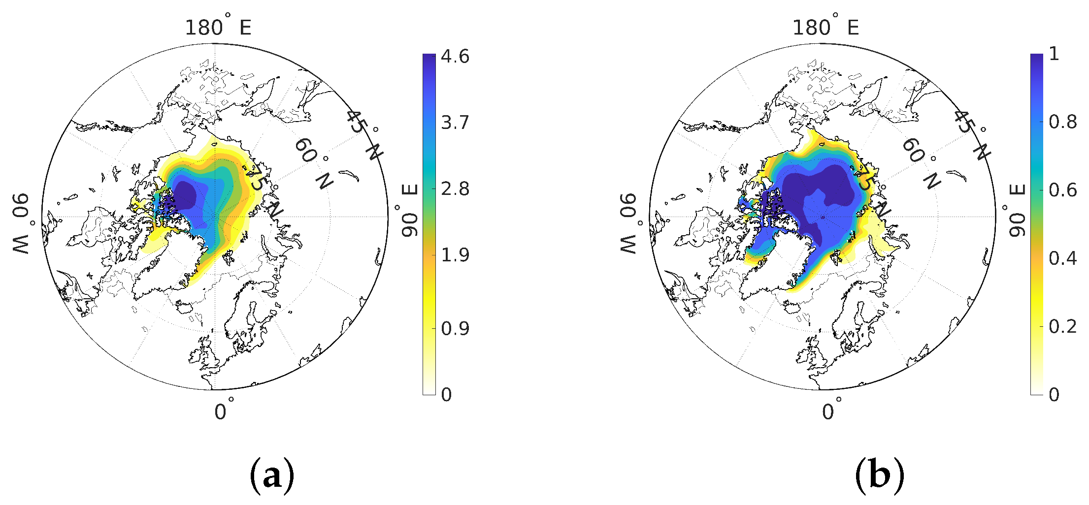
4.1. Reduction of the Ice Volume and Its Area

Under experimental conditions, with a decrease in albedo $A_1$ and $A_2$, the amount of solar radiation absorbed by the surface increases, leading to a rise in the surface air temperature. Compared to the “base” experiment $B_0$ (

Table 2. Ice volume (1) and ice extent (2) seasonal minimum in percentage relative to $B_0$ experiment. Mean surface air temperature (SAT) increment: global (3) and in Arctic (4).

Experiment	(1), %	(2), %	(3), °C	(4), °C
$A_1$	79	93	0.17	0.70
$A_2$	25	66	0.30	1.7
$C_1$	83	98	0.45	0.97
$C_2$	77	90	1.0	1.8

), the surface air temperature in $A_1$ increased by 0.7 °C in the Arctic and 0.17 °C over Earth. In $A_2$, the corresponding values are 1.7 °C in the Arctic and 0.3 °C globally. At the same time, the ice area decreased by 7% and volume by 21% in the $A_1$ experiment, while in the $A_2$, ice lost was $3/4$ of mass and 34% of its extent. In experiments with an increase in CO₂ concentration, ice melting occurs due to direct warming of the atmosphere because of the greenhouse effect. In the surface layer, the air temperature rise was approximately 0.97 °C in $C_1$, which is close to $A_1$ and approximately two times lower than in the $A_2$ experiment. However, on average, its global growth was 0.45 °C, which is substantially higher than in albedo experiments. The ice area in the $C_1$ experiment decreased by only 2.3%, and its volume reduced by 17% compared to the $B_0$ experiment. A more significant reduction in Arctic ice occurred in the $C_2$ experiment with an increase in CO₂ concentration up to 600 ppm, where its area decreased by 10% and its volume by 23%. Thus, the ice reduction is similar to the $A_1$ experiment. At the same time, the increase in averaged surface temperature is 1.0 °C, and 1.8 °C in the Arctic. Therefore, the rise in the polar area is comparable to the $A_2$ experiment with albedo.

Figure 2 shows the September (minimum) distribution of ice thickness and its compactness (fraction of the surface area covered with ice), obtained by averaging over the period 90–100 in the $B_0$ experiment. The thickest ice is concentrated in the sector of the Canadian Arctic Archipelago and is about 4.5 m. The Barents Sea is mostly free from thick ice. It is also absent in the Bering and Okhotsk Seas. In general, the picture corresponds to the observed and simulated distributions characteristic of the historical period [53].

The difference between the ice field in the series of experiments and the $B_0$ field is shown in Figure 3. Except for $A_2$, the ice thickness in experiments slightly increases in the Laptev Sea area. We can also see an increase in the Beaufort Sea area in the $A_1$ and $C_1$ experiments. The ice thickness decreases throughout the rest of the Arctic by 1–1.5 m, and in the $A_2$ experiment, by more than 2 m. In this experiment, the thickness decreases everywhere (Figure 3c). The ice compactness decreased everywhere along the Arctic Ocean’s perimeter, except a small accumulation of ice near the Taimyr Peninsula ($C_1$ and $C_2$ experiments) and in the Beaufort Sea ($A_1$ and $C_1$ experiments).

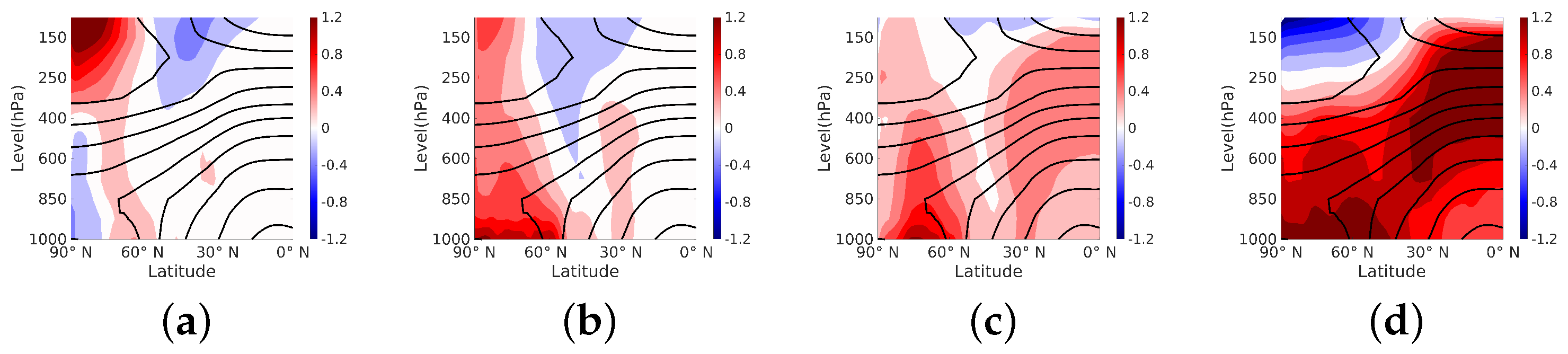
4.2. Anomalies of Zonal Temperature Distribution and Zonal Wind

The zonal distribution of atmospheric characteristics is most important in understanding its circulation. Figure 4 shows the zonal distribution of the potential temperature anomaly with altitude according to the results of these last four experiments. The distributions have some similar features. The potential temperature has a noticeable increase of about 1 °C in the lower troposphere above 60° N except for the $A_1$ experiment. Furthermore, some increase occurs in the region of 30° N, which reaches the tropopause in altitude. In the stratosphere, the temperature has a reverse tendency of decrease by about 0.2 °C in the 30–60° N band. The lower boundary of this anomaly deepens down to the level of the upper troposphere at 45–55° N.

The most noticeable difference is associated with changes in the polar part of the stratosphere. With a decrease in albedo, a positive anomaly of about 0.5–1.0 °C arose there. This difference allows us to assume that the current decrease in ice in the Arctic contributes to an anomaly in this area.

On the contrary, in the upper troposphere over the equatorial part in $C_1$ and $C_2$ experiments, near-surface tropical warming is associated with strong tropical warming in the upper troposphere. The change of moist adiabatic lapse rate can explain this result, which is similar to one in [54]. Thus, the positive anomaly is precisely a consequence of the greenhouse effect.

Figure 5 demonstrates the anomalies of the zonal velocity component. With a decrease in the ice-albedo, the zonal wind speed decreases near 50–60° N and increases in the subtropics. This structure corresponds to negative values of the Arctic Oscillation index and increased activity of Rossby waves of greater amplitude. Also, it makes the occurrence of intense and prolonged blockings in middle and high latitudes more likely. With an increase in CO₂, similar changes occur mainly in the upper troposphere, while their value is noticeably smaller in the lower troposphere. This circulation pattern is associated with an increased frequency of extreme weather events in the mid-latitude troposphere. This picture is entirely consistent with some previous studies on this issue [55,56].

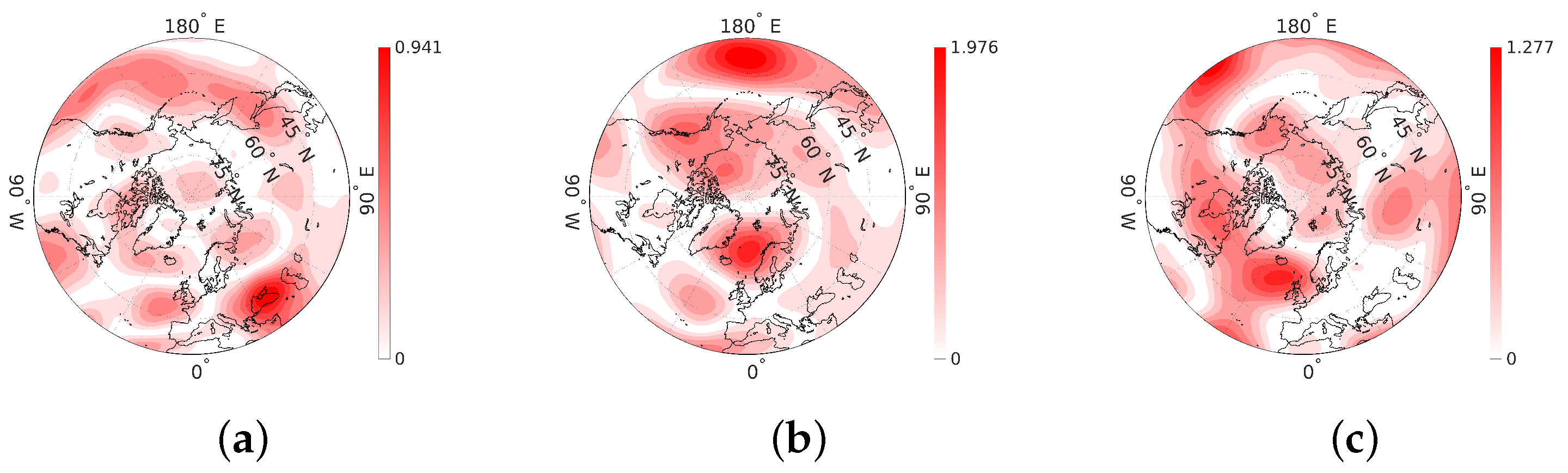
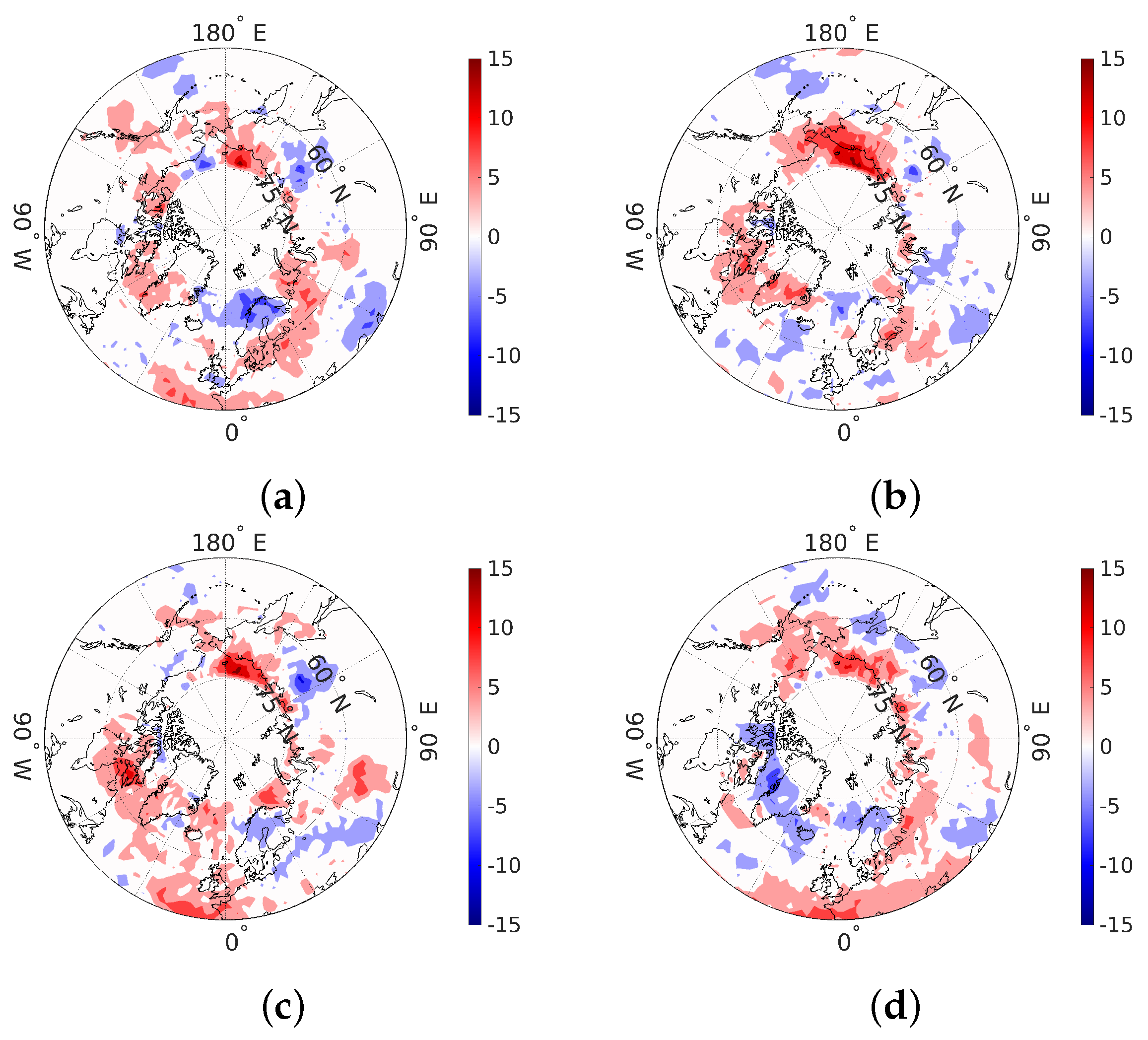
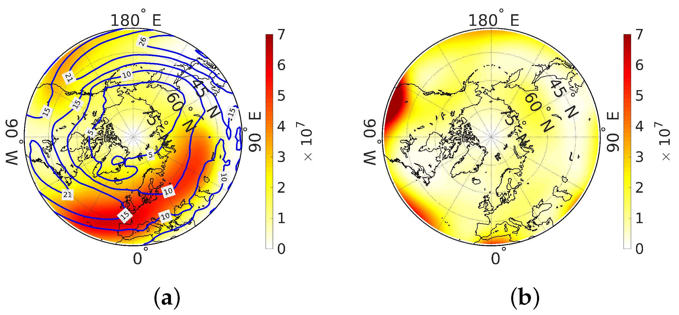
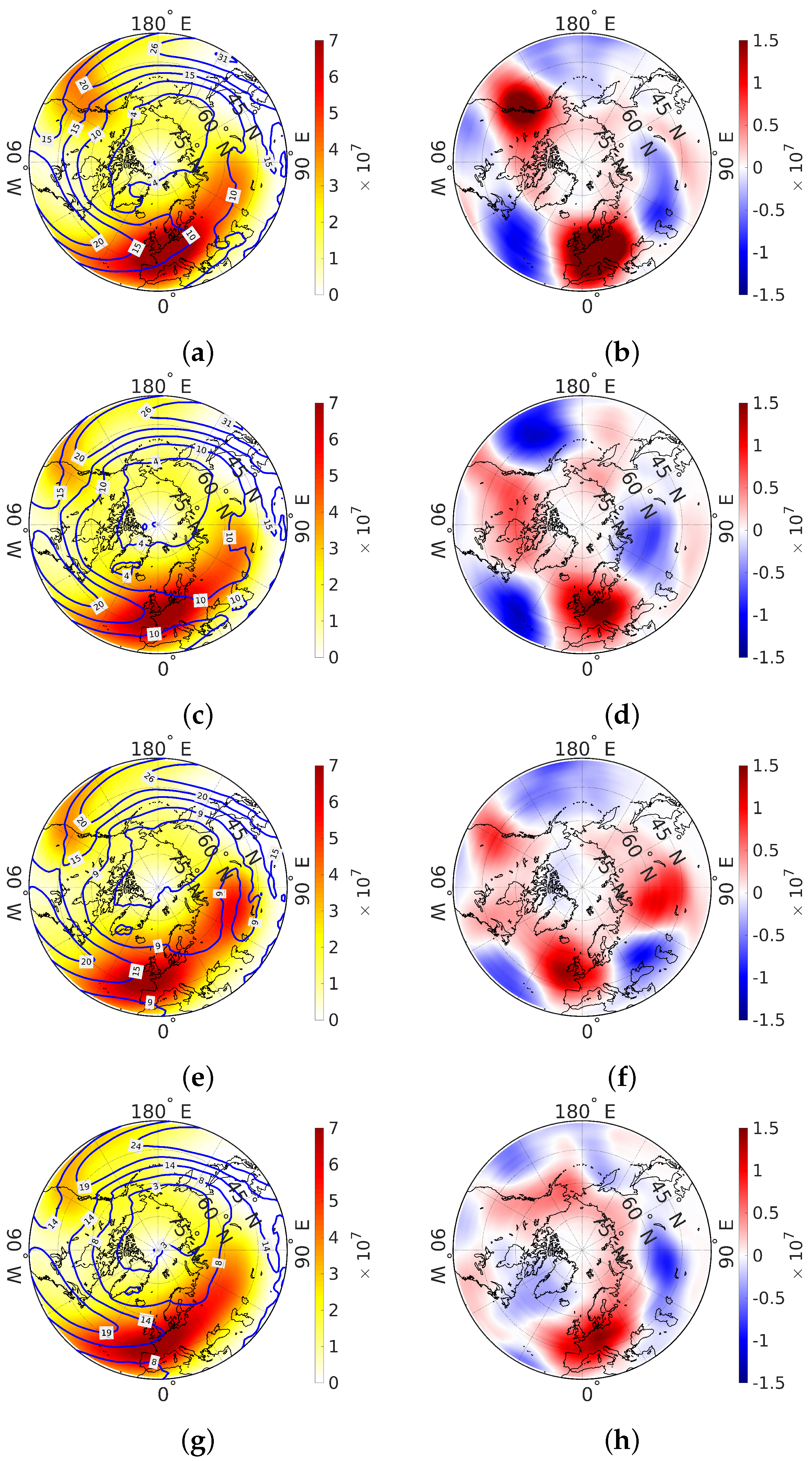
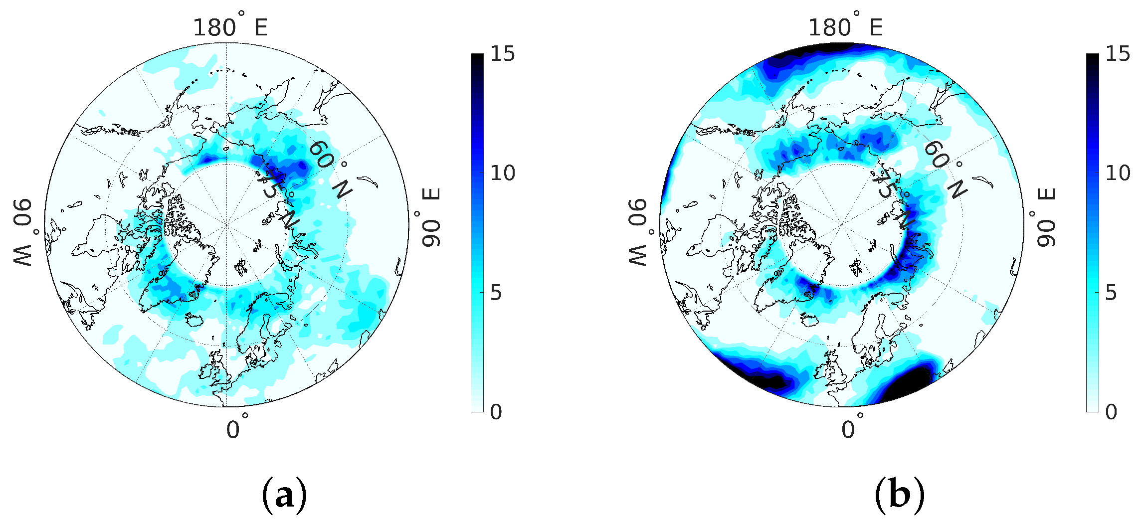
4.3. Wave Activity and Blockings

Wave activity, as defined by (6), is an objective measure for the spatial variation of physical properties and the essential diagnostics for the interaction of vortices and mean flow. Our analysis of wave activity and blockings is based on the 90–100 years of each experiment. To check the statistical significance of the resulting distributions and their trends, we used the Student’s t-test with a 5% significance level to ensure that the period of 90–100 differs from the previous period of 80–90 insignificantly. Figure 6 shows the distribution of the value t

$$\begin{array}{c}t=\sqrt{n}\frac{\overline{Z_1}-\overline{Z_2}}{s_p},\\ s_p=\sqrt{\frac{s_1+s_2}{2}},\\ s_i=\sqrt{\frac{n}{n-1}\overline{{\left(Z_i-\overline{Z_i}\right)}^2}},i=1,2,\\ \end{array}$$

(10)

where overline means sample averaging. The t value has the Student’s distribution, obtained based on the monthly average values of the value $z_{500}$ for each of the periods: $Z_1$ is a sample of the years 80–90, and $Z_2$ of the years 90–100. Thus, each sample contains $n=132$ values. The critical value of the Student’s distribution with a 5% significance level for such a sample is 1.978. In the distributions shown in the Figure 6, this value is not achieved in any of the experiments shown ($B_0$, $A_1$, $C_2$). As the Student’s t-test is subject to valid criticism, we also considered Cohen’s d-radius and Pearson’s correlation as an alternative. In the first case, the number d differs from the number t only by the multiplier $\sqrt{n}\approx 11.5$. After dividing by this coefficient, it turned out that d slightly exceeds the value of 0.2 in the central part of the Pacific Ocean and the Norwegian Sea region in the $A_1$ experiment (see Figure 6b). In the case of using Pearson’s correlation, it turned out that the value of the correlation coefficient is only slightly different from unity.

Figure 7 and Figure 8 show the anticyclonic local wave activity for the latter 11 years of each five 100-year runs.

In winter, increased wave activity is noticeable in storm tracks over the Atlantic and Pacific Oceans (Figure 7a), corresponding to the experiment $B_0$. In the albedo experiments (Figure 8a–d), the wave activity is increased over Europe and America compared to the $B_0$ experiment (Figure 7a) and decreased over the Atlantic Ocean and Asia. The response of the wave activity distribution to an increase in the concentration of CO₂ (Figure 8e–h) is similar over Europe but qualitatively different elsewhere. In the $C_1$ experiment, the wave activity significantly increases over Asia and America, while in the $C_2$ experiment, the change in wave activity over America is small and becomes negative over Asia.

In summer (Figure 7b), the maximum wave activity is in the subtropical latitudes. The difference between experiments is insignificant (not shown).

Figure 8 also demonstrates the shift of wave activity in the eastern direction, which may indicate a displacement of storm trajectories to the east. Blocking phenomena often occur at the outlet of jet stream zones onto the continent, such as over the northeastern North Atlantic and the eastern Pacific (see in [57]). Comparing the results shows that the decrease in wave activity over the Atlantic Ocean in the albedo experiments corresponds to a reduction in the blocking number. The area of storm trajectories over the Pacific Ocean is almost unchanged: the number of blockings and the magnitude of wave activity remain approximately at the same level. In addition, note that all experiments demonstrate the peak of wave activity in western Europe, which also corresponds to the reanalysis data showing the predominance of anticyclonic circulation in this region [46]. In [58], authors noted that the process of blocking formation in the North Pacific Ocean might differ from that in the Euro-Atlantic sector, and that, while in the formation of North Pacific blocking, non-stationary eddies of synoptic-scale play a vital role, blocking in the Euro-Atlantic region is caused by quasi-stationary waves. Thus, these results suggest that the wave activity flux associated with stationary (or quasi-stationary) Rossby waves is of paramount importance for the blocking process over Europe. In contrast, the influence of non-stationary synoptic-scale processes is necessary for this over the North Pacific Ocean.

Stationary waves ultimately arise from asymmetries on the Earth’s surface, mountains, continent–ocean contrasts, and sea surface temperature asymmetries. Understanding strictly how stationary waves are created and maintained is a fundamental challenge in climate dynamics. Wave amplitudes in the northern hemisphere are most remarkable in winter, moderate in the transitional seasons of spring and autumn, and weakest in summer.

Stationary waves play a crucial role in block formation, but the onset of the blocking process is still poorly understood and remains a challenging problem. Due to incomplete understanding, the mechanisms of blocking formation remain somewhat subjective, and the various blocking indices are not always consistent with the impact of climate change on them.

In [57], the authors considered a mechanism for atmospheric jet blocking at mid-latitudes, similar to the traffic jam problem. They suggested a local wave activity (LWA) of finite amplitude, as an estimate of potential vorticity waviness, based on the interaction theory between waves and mean flux. It was pointed out that the relationship between LWA and block formation is based on several properties of LWA, particularly on a quantitative assessment of the mutually compensating tendency between the meandering of the jet stream and the speed of the western stream. In our work, to assess the relationship between LWA ($A_N$) and U (zonal wind), we also calculated the temporal covariance field between LWA and U (both at 500 hPa) for the winter season (December–February), averaged over the last 15 years of modeling. The covariance turned out to be negative everywhere (Figure 9a) in $B_0$ as well as in other experiments: that is, when the jet strongly meanders, the western flow slows down (and sometimes changes to the eastern one). The scatterplots (Figure 9b,c) show the mutually compensating trends in LWA and zonal velocity in Atlantic and Pacific extremal points of the $B_0$ experiment. Figure 9a shows the position of these points. These trends suggest an approximate relationship $A_N\approx A_0-kU$, where $A_0$ and k are positive constants. The red lines in Figure 9b,c are constructed by the least-squares method as a best linear fit for all events.

Table 3. Points of highest correlation between $A_N$ and U in Atlantic and Pacific oceans in 30–50° N latitude band for experiments with the values of corresponding regression coefficient k in these points.

Experiment	Atlantic Ocean		Pacific Ocean
	Coordinates	k, m·s 107	Coordinates	k, m·s 107
$B_0$	42 N, 28 W	−1.06	42 N, 148 W	−1.15
$A_1$	40.5 N, 26 W	−1.21	39 N, 136 W	−1.28
$A_2$	46.5 N, 4 W	−0.73	36 N, 178 W	−3.8
$C_1$	45 N, 12 W	−0.99	37.5 N, 122 W	−0.94
$C_2$	45 N, 18 W	−1.37	36 N, 162 W	−2.44

summarizes the corresponding coordinates of extremal points in the Atlantic and Pacific oceans along with the value of regression coefficient k in these points.

Figure 10, Figure 11 and Figure 12 show the blocking rate in terms of the number of blocking events defined according to criterion (7) and (8) over the last 11 years of the experiment.

In winter (December–February), the conditions for the formation of blockages most often occur around the pole, on average being limited to latitude 60° N, but at the same time reaching central Europe, the southern Urals, and Kazakhstan (Figure 10a). The highest frequency, in this case, falls on the territory of Yakutia and the Chukchi Sea, reaching 15 blockages for all winters of 10 years (i.e., on average, 1.5 blockings per winter). Furthermore, blockages are frequent in Greenland, the Norwegian Sea, and Kazakhstan—up to 5–10 events. We can also note the probability of blocking in the North Pacific and Atlantic Ocean (2–3 events) along storm tracks.

In the case of an increase in CO₂ concentration to 450 ppm in experiment $C_1$ (Figure 11c), when the decrease in the ice field is slight, the number of blockages increases by 10–15 events in the region of the East Siberian Sea and the Canadian Arctic Archipelago (CAA), by 5–10 events in the north-western Atlantic, the south of the Barents Sea, Kazakhstan and the south of western Siberia. At the same time, it decreases noticeably (by 5–10 events) in Yakutia and Eastern Europe. With an even more significant increase in CO₂ concentration in the $C_2$ experiment (Figure 11d), a belt of positive change in the blocking frequency is formed, extending from Europe and the adjacent part of the Atlantic and further along the Arctic coast of Eurasia to Alaska. In this case, the CAA region falls into the zone of reducing the number of blockings.

The reduction of the ice field in the $A_1$ experiment is approximately the same as in the $C_2$ experiment (see Table 2 and Figure 3). Therefore, the tendencies in blocking frequency (Figure 11a) almost entirely coincide with experiment $C_2$, except for CAA. In contrast to $C_2$, the number of blockings increases by 5–10 events here. With an even greater decrease in albedo in $A_2$ and a significant reduction in ice, the picture of the change in the blocking conditions in $A_2$ looks more different (Figure 11b). In almost the entire ring in the region of 65–70° N, the number of blockages increases by 5–15 events, including CAA. An exception is the Norwegian and Greenland Seas region, where we can observe a decrease of about 5 events, as for the central regions of the North Atlantic. The exact change is seen for the south and north of eastern Europe, the south of eastern Siberia, and the central part of the Pacific Ocean.

Thus, the general features of changes in the blocking conditions are (1) an increase in the number of blockages in the region of the East Siberian and Chukchi Seas, including Alaska; (2) the growth of blocking number in central and eastern Europe; (3) reducing the number of blockages in the area of northern Scandinavia and the Norwegian Sea; (4) decrease in the Caspian region and Kazakhstan; and (5) decrease in the region of Yakutia. The CAA region demonstrates an ambiguous change in the blocking frequency: an increase in experiments $C_1$, $A_1$, and $A_2$, and a decrease in experiment $C_2$. The difference could be due to the peculiarities of one or another method of ice reduction in numerical experiments and the nonlinearity of the climate system’s response to disturbances. These trends are generally consistent with the comprehensive analysis of winter and summer atmospheric blocking processes in the Northern Hemisphere presented in [53], based on the results of modeling using three generations of climate models: CMIP-3 (2007), CMIP-5 (2012), and CMIP-6 (2019). Most of the models show that a decrease in the frequency of winter blocking is expected in the coming decades everywhere, except for western North America. Our results in association with sea ice reduction also show an increase in central and eastern Europe and the Pacific sector of the Arctic.

Summer (June–August) blocking frequency distribution for the base experiment $B_0$ is shown in Figure 10b. The areas with the most frequent blockages form two rings. The first is around the pole at a latitude of approximately 65–70° N and roughly corresponds to the Arctic Ocean’s coastline. Three zones with the highest frequency of blocking events can be distinguished here: in the Barents-Kara-Laptev seas, on the Arctic coast of Chukotka and Alaska, and the Greenland region. These are blockings occurring on the northern flank of the jet stream. The second ring adjoins the subtropics and corresponds to the blockings forming on the southern flank. In subtropical latitudes, the number of blockings is much greater in summer when anticyclonic vorticity prevails. The most significant number of blocking events can be noted in the North Atlantic and North Pacific regions along storm tracks and the western parts of Europe and America, where they hit the continent. At the same time, vast areas of Central Asia are on the sidelines of these events.

With a decrease in albedo in the $A_1$ and $A_2$ experiments within the first ring (Figure 12a,b), the blocking frequency noticeably decreases on the line of the Barents-Kara-Laptev seas, but at the same time, it strongly increases to the east of it in the Yakutia region. The blockage rate also increases in the second area, covering the entire Bering Sea. The probable cause of this increase is the growth of wave activity due to a decrease in the gradient. However, the blockage rate decreases in the Greenland region. In the second ring, a noticeable increase in frequency in the $A_1$ experiment, when the reduction of the ice field is less significant, takes place in northeastern Europe and the northeastern part of the Pacific Ocean. In the Atlantic, the number of blockages is decreasing. With a significant reduction in the ice field in the $A_2$ experiment, these changes are less pronounced, but the frequency decreases noticeably in the central part of the Pacific Ocean.

The changes are similar with an increase in CO₂ in the first ring (Figure 12c,d). However, in the Chukotka and Alaska region in the $C_1$ experiment, there is a slight decrease in the blocking frequency, and in the $C_2$ experiment, the distribution of trends in this area is spotty and close to neutral. The second ring also shows an increase in blockages in eastern Europe and the northeast Pacific and a decrease in the North Atlantic. Thus, except for the region of Chukotka and Alaska, the summer trends of the $A_1$ and $A_2$ experiments coincide with the $C_1$ and $C_2$ trends. This fact allows us to assume that the indicated tendencies are caused precisely by the reduction of the Arctic ice. We can also assume that with a slight increase in the concentration of CO₂ ($C_1$), when the ice field changes insignificantly, the trend in the frequency of blockages in the Chukotka and Alaska region is negative. However, with a further increase in the CO₂ concentration ($C_2$), when the decrease in Arctic ice becomes more significant, an opposite trend, which eventually compensates for the previous one, is activated in this area. This trend is similar to $A_1$ and $A_2$ experiments. In the analysis by the authors of [53], summer blocking frequency decreases almost everywhere except for the Ural; the slight manifestation of the latter can be seen in the $C_2$ experiment.

Along with the blocking frequency, an essential characteristic of this phenomenon is its intensity. The blocking intensity depends on the relative elevation of the maximum of the geopotential height. As before, we will use the $z_{500}$ characteristic. If, first, we assume an $\mathsf{\Omega }$-type blocking structure, then the line connecting two adjacent minima of $z_{500}$ at the midpoint will have $z=(Z_u+Z_d)/2$, where $Z_u$ and $Z_d$ are $z_{500}$ values at the upstream and downstream points of minimum. Then, the elevation of the maximum above this line can be estimated by taking the difference $Z_{\max }-z$. If we take the ratio of this value with the average $(Z_{\max }+z)/2$, then we get the relative elevation. When we are dealing with Rex-type blocking, one of the lows can be far away. Therefore, one can take the $z_{500}$ value at a certain distance from the high. The very idea underlies the $BI$ blocking intensity index proposed in [59]. For each coordinate point $\left(\lambda ,\varphi \right)$ where a blocking event is detected according to (7), we define $BI$ as

$$BI\left(\lambda ,\varphi \right)=100\%\frac{-Z_u+2Z-Z_d}{Z_u+2Z+Z_d},$$

(11)

where $Z=z_{500}\left(\lambda ,\varphi \right)$, and $Z_u$ and $Z_d$ are the minimum values of the $z_{500}$ field within $\lambda$ ± 60° upstream and downstream at $\varphi$ latitude, respectively.

In the expression (11), if we assume that $Z_u=Z_d=\overline{Z}(1-\alpha )$ and $Z=\overline{Z}(1+\alpha )$, then we get that $BI=100\%\alpha$. Thus, we can interpret the $BI$ value as the amplitude of the sawtooth change in the geopotential height in the blocking region. We can say approximately the same about pressure, so the pressure drop in the blocking area will equal $p=500·(1\pm \alpha )=500·(100\%\pm BI)$ hPa. By definition, $BI$ is always positive. The higher the $BI$ index, the greater blocking intensity. If at some point $BI=0$, then there is no blocking.

Figure 13 demonstrates the distribution of the average blocking intensity obtained over the last 11 years of the $B_0$ 100-year experiment separately for winter (December–February) and summer (June–August). Comparing this figure with the blocking frequency Figure 10, we can see that they are almost negatives of each other. That is, the more frequent the blockings, the less intense they are, and vice versa.

We note that in winter (Figure 10a and Figure 13a) the most intense blockings are $BI\approx$ 7% with pressure drops at an altitude of 5.5 km (approximately corresponds to $z_{500}$) about 500 ± 35 hPa are formed in the eastern part of the Pacific Ocean. However, during the 11 years under consideration, these events occurred only 1–2 times. Blockings of the same intensity occur in the eastern Atlantic near the British Isles, but these events happen 2–3 times more often. The Ural blocking, which forms approximately at the longitude of the Ural Mountains, corresponds to $BI$ ≈ 2–4% and occurs about once every 1–2 years. Roughly the same picture is evident for the blocking in the Greenland region. For areas with the maximum frequency of blockings (Yakutia and the Chukchi Sea), their intensity is only 1–2%. Figure 14 shows trends associated with changes in blocking intensity in experiments $A_1$, $A_2$, $C_1$ and $C_2$. We can note that the results of almost all experiments indicate a decrease in the intensity of blockings near the British Isles by 3–6% and an increase by the same 3–6% in northeastern Europe. We can interpret these changes as a displacement of the center of intensity to the east and increased Ural blocking. Based on the analysis of the results of six experiments using different climatic models [60] noted an increase in the Siberian maximum and a weakening of the Icelandic minimum, both changes are going along with strengthening the Ural blocking and decline of blocking intensity in the western part of the North Atlantic. On the other side of the Arctic, the intensity of blockings is increasing in Alaska, and the Sea of Okhotsk, which is also supported by [60] finding of the Aleutian Low strengthening.

In summer (Figure 10b and Figure 13b) the intensity of blocking decreases and the maximum value is only 3.4% (i.e., 500 ± 17 hPa). Such blockings occur at a latitude of approximately 50–55° N. Note that, as a rule, the places of their formation are at the edge of the zones of the highest frequency (Figure 10b), namely, in the Aleutian Islands, southern Alaska and British Columbia, American Lakes, the central part of the North Atlantic, and Central and Eastern Europe. These events occur about 2–3 times every 11 years. We can note less intense (2.5–3%) blockings with the same frequency in the east of Asia near the Sea of Okhotsk. More frequent blockings that form along the Arctic coast are even less intense, and their $BI$ index is only 1–2%.

The most significant increase in the intensity of blocking in summer by 1–2% (Figure 15) in the experiments $A_1$, $A_2$, $C_1$, and $C_2$ we can note in the area of the Greenland, Norwegian, and Barents seas, and also near the Bering Strait and the Chukchi Sea, i.e., in places directly related to the retreat of the ice field. At the same time, a decrease in intensity by about 1% in the CAA region and Yakutia can be noted.

5. Discussion

In the experiments with decreased albedo, the zonal wind speed decreases near 55–60° N. A weakening of the polar potential vorticity gradient in the lower stratosphere near the tropopause goes along with this speed reduction. Furthermore, in the subtropics, the zonal wind increases. In this case, the meandering of the jet flow grows, which can be measured by the value of LWA. Persistent high LWA values may indicate a high probability of blockage in the atmosphere. Jet blocking is an anomalous weather event, so it is not surprising that high LWA values are associated with geopotential height anomalies. Thus, understanding the jet flow dynamics and what factors might affect the LWA values can provide insight into extreme weather conditions and help quantify the interaction of mean vortex flows on a regional scale. In addition, insights are emerging on how climate change can affect atmospheric dynamics at mid-latitudes. For blocking to occur, the LWA values must exceed the wave break threshold.

Typically, the geopotential height increases with the anticyclonic LWA and decreases with the cyclonic LWA. As the anticyclonic LWA is higher than the cyclonic LWA, this increases the geopotential height with the LWA in most locations.

In the case of a decrease in albedo, the LWA distributions change significantly with an increase in wind shear in the stratosphere (Figure 5). As the wind shear increases, the LWA values increase. This result is quite reasonable given that an increase in wind shear leads to a rise in eddy activity caused by growing baroclinic instability and an increase in the LWA values and blocking frequency.

While there is no universally accepted definition of blocking, most researchers today identify them as ridges in a jet stream that persist for five days or more. In recent studies, the inversion of the $z_{500}$ geopotential height gradient and the potential vortex at mid-latitudes are most often used to identify blocking events. Our work also used these identification methods. However, note that as the models have their drawbacks, they cannot describe some aspects of the physics of the process associated with the life cycle of blocking development, including large-scale interactions.

One of the known problems associated with blocking is its substantial natural variability, including, for example, a small number of rare but persistent and significant events. This variability has several practical implications. For example, it often takes long periods or several members of the modeling ensemble to get good blocking statistics. Given the level of natural variability, observations have not yet possibly revealed any entirely consistent long-term trends in blocking. Considering the importance of natural variability for mid-latitude circulation in general (see, e.g., in [61]), it is likely that it will continue to play a leading role in blocking change over the next few decades.

Determining the blocking itself has become a significant problem because different blocking indices target different block characteristics. Blocking has always been a problem for weather forecasts and climate models because of its specific nature, which is difficult to simulate correctly numerically [44]. Several generations of climate models have shown significant negative deviations in blocking frequency, especially in the European sector (see, e.g., in [24]). However, there is general agreement that blocking rates should decrease in the next century [24], but this may depend on the index used. Moreover, observations can hardly confirm any trend [35,46].

Choosing a blocking index is a necessary and fundamental step for this job. There are indices based on flow topology and determined through model or observed meridional gradients of the geopotential or potential vortex (see, e.g., in [27,44]) that we use in our work, but there are other types of indices (see, e.g., in [24,34]).

The analysis of the blocking intensity showed that in the experiments, as a result of the reduction of the Arctic ice, the intensity maximum near the British Isles shifts to the east, thereby strengthening the winter Ural blockings by 3–6%. In [62], the authors examined the relationship between Ural blocking and the background conditions associated with the Arctic warming over the Barents and Kara Seas and found that the intensity of Ural blocking is significantly related to this warming. In winter, the intensity of blockings in the Alaska region and the Sea of Okhotsk also increases. In summer, the changes in intensity are not significant, about 1%, and mainly concern the areas affected by ice retreat.

Comparing blocking frequency and blocking intensity shows that the more frequent the blockings, the less intense they are. In this respect, it is interesting to consider the field built as the product of the last two. It will give us an idea of where the transitions of wave energy into blocking energy occur.

Figure 16a shows that such energy transformations occur in the following regions: northern Scandinavia, Yakutia, the Chukchi Sea, Greenland, eastern Aleutian Islands, the British Isles region, and Kazakhstan. Moreover, in the first four regions, blockings are more frequent but less intense. In the rest, on the contrary, blockings are higher in intensity but occur less frequently.

In experiments with the reduction of Arctic ice (Figure 17), we can identify the following general tendencies: weakening of processes in the vicinity of the British Isles and Kazakhstan, with a simultaneous increase in northern Europe and the Urals; weakening in the east of the Aleutian Islands and strengthening in the region of Alaska and the Sea of Okhotsk. All the tendencies noted are associated with an increase in energy of blockings in the northern areas, with a simultaneous decrease of the southern ones.

In summer (Figure 16b), in addition to the regions adjacent to the subtropics in the central part of the Pacific and the Atlantic Ocean and southern Europe, the Arctic part can also be distinguished: the line of the Barents-Kara-Laptev Seas, the Kolyma basin, and northern Alaska. As a result of ice reduction in Figure 18, one can distinguish the following summer trends: weakening in the areas mentioned above close to the subtropics, weakening along the line of the Barents-Kara-Laptev Seas, and strengthening in the Bering and Chukchi Seas. There are ambiguous trends in the Greenland and Norwegian Seas, Beaufort Sea, and Kolyma basin. In Eastern Europe, the growth is mainly, but it becomes insignificant with 75% of ice mass lost in $A_2$. The central parts of the North Pacific and Atlantic are also associated with storm tracks which generally run in these sectors. Surface orography contributes to the difference in spatial structures of storm trajectories through stationary Rossby waves [63,64,65].

Storm tracks are usually more active in winter than in summer when pole-equator and continent-ocean temperature gradients increase baroclinicity. However, the suppression of storm activity in the North Pacific in midwinter is a notable exception [66]. In both storm track regions, poleward heat flux at the lower levels is the primary source of LWA. However, the compensating mechanisms are different. Our simulation results show that LWA and zonal wind have negative covariance in the Atlantic and Pacific. This fact suggests that the blocking maxima occur near the stationary high-pressure anomalies at the exit of the storm track region.

Comparing the action results of two mechanisms (experiments $A_1$–$A_2$ and $C_1$–$C_2$), leading to a decrease in Arctic ice, one can see certain similarities and differences. With an increase in the concentration of CO₂ in the atmosphere and melting of ice as a result of this increase, the effective albedo of the underlying surface in the Arctic inevitably decreases, as leads and melt ponds appear, and the snow surface becomes darker due to an increase in water content. The INM-CM48 parameterizes these processes by changing surface albedo according to (9). Therefore, experiments $C_1$ and $C_2$ have features in common with experiments $A_1$ and $A_2$, associated with ice reduction. However, in addition to this, an increase in CO₂ concentration entails, as can be seen from Table 2, significant heating of atmospheric air, and the unevenness of this heating further sharpens or smooths out the zonal gradients, and this is no longer associated with a decrease in the amount of ice. Therefore, analyzing the results of experiments $C_1$ and $C_2$, we cannot attribute the consequences exclusively to changes in the ice. Experiments $A_1$ and $A_2$ with an artificial decrease in albedo also have several consequences not related to changes in ice, as here the natural radiation balance on the surface is disturbed, as a result of which, as again follows from Table 2, one can also note an increase in the surface air temperature, although not so significant as in experiments $C_1$ and $C_2$. Other consequences are also possible, which are difficult to predict in advance.

Atmospheric blockings in the northern hemisphere in winter and summer were also the focus of the climate model intercomparison project. It compared data from CMIP5 (2012) and CMIP6 (2019) to different reanalysis datasets. This extensive analysis provided insights into the ability of general circulation models to reproduce atmospheric blocking in today’s climate and evaluate it in future scenarios [67].

Analyzing the similar features of the resulting distributions, we can assume that they result from ice reduction, which we would like to obtain. However, they can also result from increased air temperature or other mutual consequences of the two mechanisms. If an increase in temperature causes the similarity of the consequences, their manifestations in experiments $C_1$ and $C_2$ would be brighter as the increase in temperature is more significant in these experiments. However, as we can see from the presented results, this is far from the case. Therefore, we tend to attribute similar features to the effects of ice reduction. Nevertheless, it is not possible to unequivocally prove this, so we can only talk about the possibility of such interconnections. Based on this, we can assume that the following changes in the atmosphere and its dynamics are associated with the reduction of ice in the Arctic:

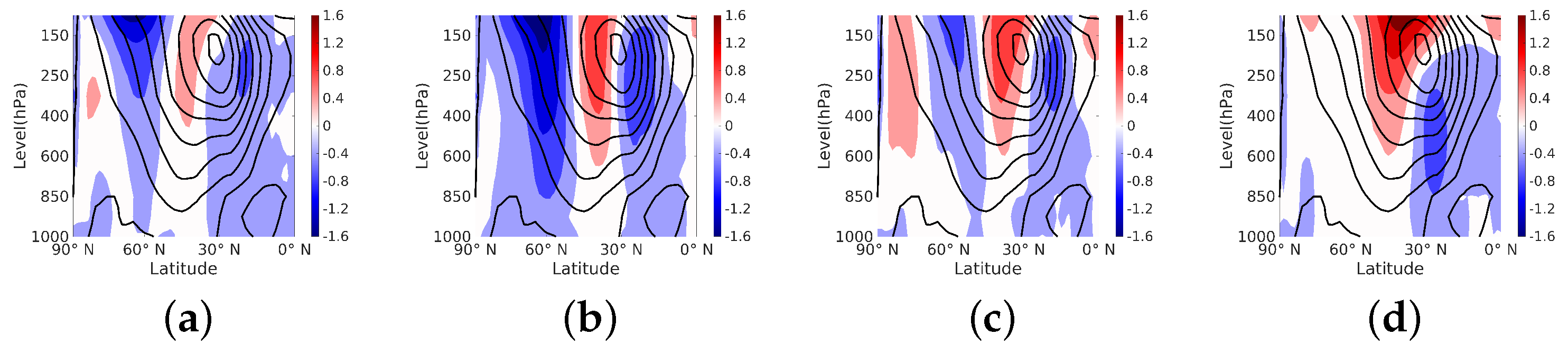
• Increase in tropospheric temperature at latitude 60–70° N, and a decrease in stratospheric temperature at latitude 40–50° N, both cause a reduction in the gradient at the tropopause level in mid-latitudes. An increase in the temperature of the upper troposphere at latitude 20–30° N, and consequent increase in the gradient at the tropopause level at latitudes 30–40° N (Figure 4).
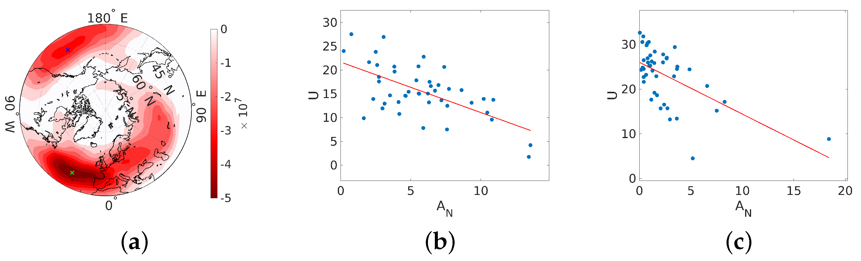
• Acceleration of the zonal flow at latitude 30–50° N, decelerating the flow at latitude 20–30° N. It means a shift of the jet to the north. Acceleration of eastern transport at latitude 80° N (Figure 5).
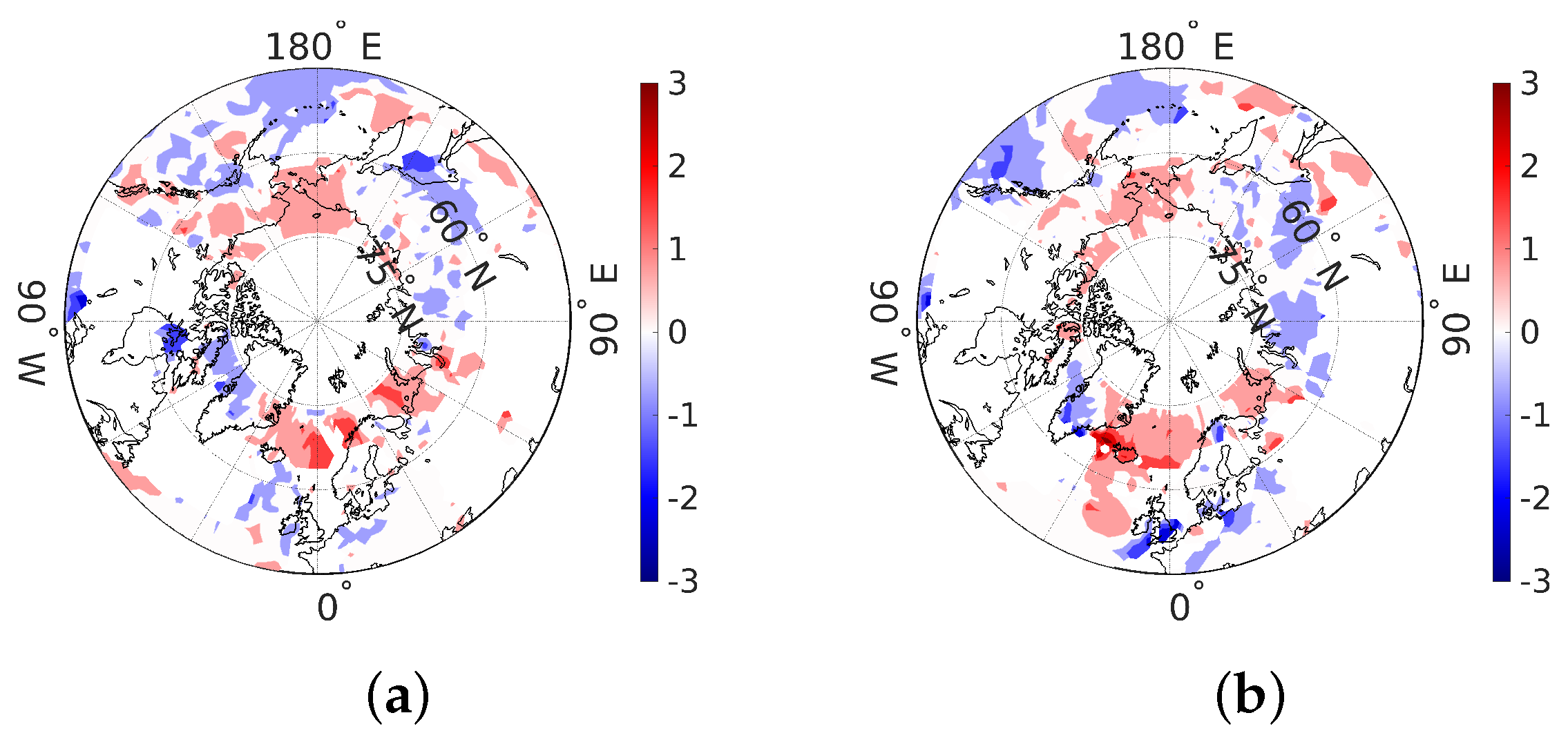
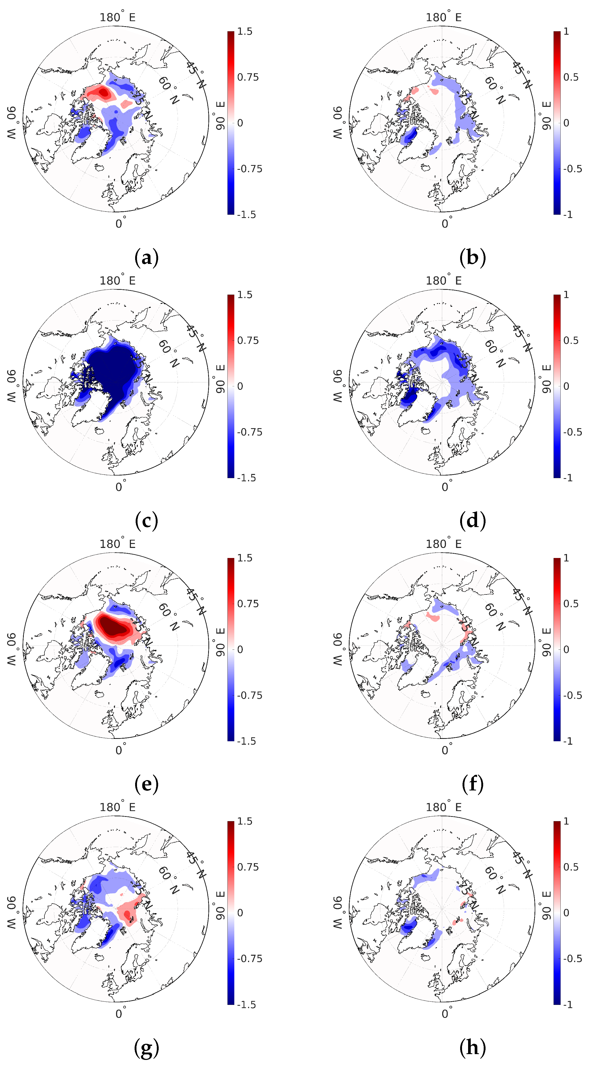
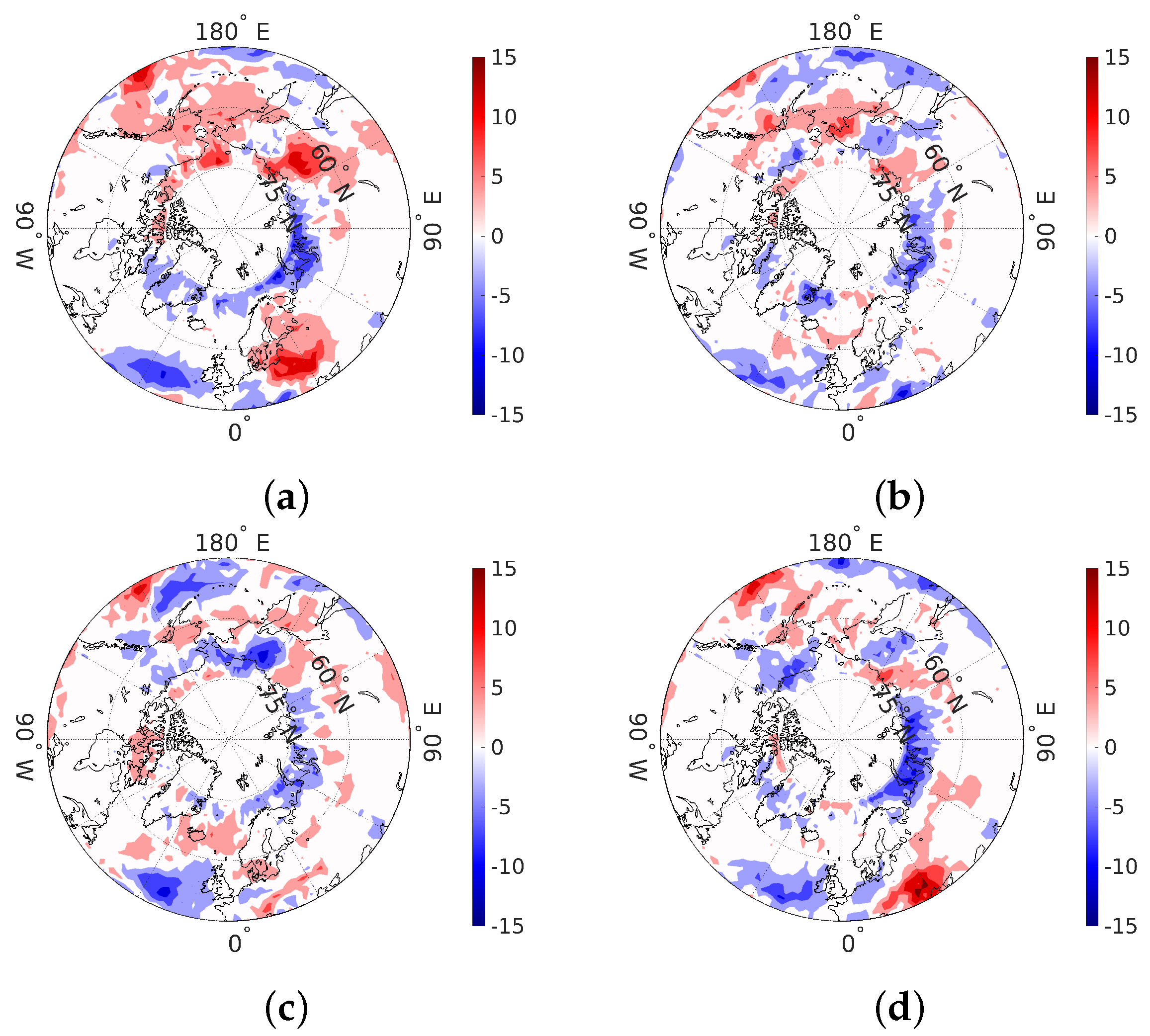
• Intensification of wave activity in Europe, Western America, and Chukotka, and its weakening in the south of Siberia and Kazakhstan (Figure 8).
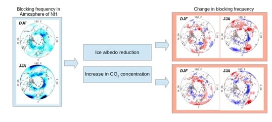
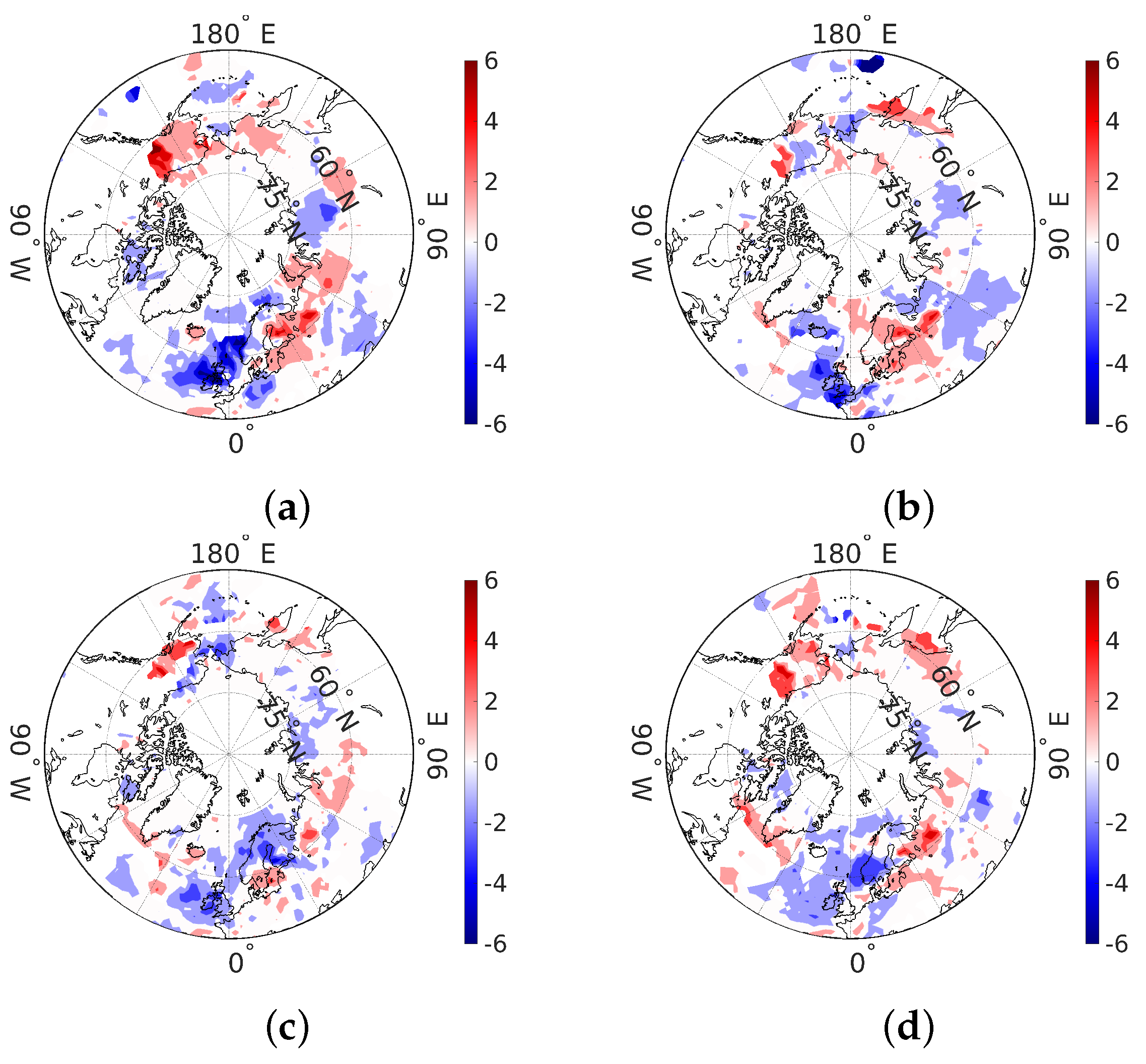
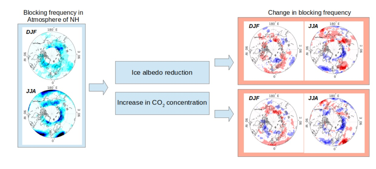
• Winter increase in the number of blockings in the East Siberian and Chukchi Seas, including Alaska, in central and eastern Europe and the reduction in blockings in the Norwegian Sea, Caspian region and Kazakhstan, and Yakutia (Figure 11).
• Summer decrease in the number of blockings on the line of the Barents-Kara-Laptev seas, in the Greenland region, in the central Atlantic and Pacific Oceans, but increase in the Yakutia, in northeastern Europe and the northeastern part of the Pacific Ocean (Figure 12).

In addition to the similar features resulted from the $A_1$–$A_2$ and $C_1$–$C_2$ experiments, there are significant differences that also make sense to list:

• With minor changes in albedo, an increase in the polar stratospheric temperature (>1 °C), and with a significant increase in CO₂ concentration, its decrease (1 °C);
• The temperature rise at the border of the troposphere and stratosphere in the tropics takes place only with an increase in the concentration of CO₂.
• The deceleration of the flow at latitude 50–65° N occurs only with a decrease in albedo and disappears with an increase in CO₂.
• Weakening of wave activity in the central part of the oceans in $A_1$. Weakening in the northwestern part of the oceans in $C_2$, while in $A_1$, there is an increase.
• Winter increase in the number of blockings occurs in CAA in experiments $C_1$, $A_1$, and $A_2$, while in experiment $C_2$ number of blockings decreases.
• Summer increase in the number of blockings occurs in the entire Bering Sea in $A_1$ and $A_2$, while in the $C_1$ there is a slight decrease in the blocking frequency, and in the $C_2$ there is no significant trend.

If we talk about an increase in CO₂ concentration as the main factor causing recent climatic changes, then the differences indicate the processes in the atmosphere, which are (most likely) directly caused by an increase in the amount of CO₂ in the air and are not associated with changes in the ice field.

6. Conclusions

This paper considers a series of numerical experiments to identify the direct role of the Arctic sea ice reduction process in establishing trends in the northern atmosphere circulation. Aimed at this, we used two mechanisms of ice reduction: an increase in the concentration of carbon dioxide in the atmosphere and a reduction in the reflectivity of ice and snow. The most prominent consequences of ice reduction, as a result of numerical tests, were the weakening of temperature gradient at the tropopause level in mid-latitudes; the zonal wind speed decrease near 50–60° N and its increase in the subtropics; and intensification of wave activity in Europe, Western America, and Chukotka, and its weakening in the south of Siberia and Kazakhstan. Changes in wave activity lead to changes in the frequency and intensity of blockings. We used a modified blocking criterion to evaluate the simulated blocking frequency and blocking intensity for north hemisphere mid-latitude regions in winter and summer, corresponding to ice reduction. In experiments with the reduction of Arctic ice, we can identify the following general tendencies associated with winter blockings: their weakening in the vicinity of the British Isles and Kazakhstan, with a simultaneous increase in northern Europe and the Urals; weakening in the east of the Aleutian Islands and strengthening in the region of Alaska and the Sea of Okhotsk. These tendencies mean an increase in energy of blockings in the northern areas, with a simultaneous decrease of the southern ones. The summer trends include weakening in areas close to the subtropics, weakening along the Barents-Kara-Laptev Seas, strengthening in the Bering and Chukchi Seas. Furthermore, blockings strengthen in Eastern Europe, but extreme ice loss makes this strengthening insignificant.

References

1. Andersen, J.K.; Andreassen, L.M.; Baker, E.H.; Ballinger, T.J.; Berner, L.T.; Bernhard, G.H.; Bhatt, U.S.; Bjerke, J.W.; Box, J.E.; Britt, L.; et al. The Arctic. Bull. Am. Meteorol. Soc. 2020, 101, S239–S286. [Google Scholar] [CrossRef]
2. Wills, R.C.J.; White, R.H.; Levine, X.J. Northern Hemisphere Stationary Waves in a Changing Climate. Curr. Clim. Chang. Rep. 2019, 5, 372–389. [Google Scholar] [CrossRef] [PubMed] [Green Version]
3. Wu, B.; Handorf, D.; Dethloff, K.; Rinke, A.; Hu, A. Winter Weather Patterns over Northern Eurasia and Arctic Sea Ice Loss. Mon. Weather Rev. 2013, 141, 3786–3800. [Google Scholar] [CrossRef] [Green Version]
4. McIntyre, M.E.; Palmer, T.N. Breaking planetary waves in the stratosphere. Nature 1983, 305, 593–600. [Google Scholar] [CrossRef]
5. Polvani, L.M.; Saravanan, R. The Three-Dimensional Structure of Breaking Rossby Waves in the Polar Wintertime Stratosphere. J. Atmos. Sci. 2000, 57, 3663–3685. [Google Scholar] [CrossRef]
6. Kim, B.M.; Son, S.W.; Min, S.K.; Jeong, J.H.; Kim, S.J.; Zhang, X.; Shim, T.; Yoon, J.H. Weakening of the stratospheric polar vortex by Arctic sea-ice loss. Nat. Commun. 2014, 5, 4646. [Google Scholar] [CrossRef] [Green Version]
7. Sun, L.; Deser, C.; Tomas, R.A. Mechanisms of stratospheric and tropospheric circulation response to projected Arctic sea ice loss. J. Clim. 2015, 28, 7824–7845. [Google Scholar] [CrossRef]
8. Strong, C.; Magnusdottir, G.; Stern, H. Observed feedback between winter sea ice and the North Atlantic Oscillation. J. Clim. 2009, 22, 6021–6032. [Google Scholar] [CrossRef]
9. Deser, C.; Tomas, R.; Alexander, M.; Lawrence, D. The seasonal atmospheric response to projected Arctic sea ice loss in the late twenty-first century. J. Clim. 2010, 23, 333–351. [Google Scholar] [CrossRef] [Green Version]
10. Sévellec, F.; Fedorov, A.; Liu, W. Arctic sea-ice decline weakens the Atlantic Meridional Overturning Circulation. Nat. Clim. Chang. 2017, 7, 604–610. [Google Scholar] [CrossRef]
11. Drijfhout, S. Competition between global warming and an abrupt collapse of the AMOC in Earth’s energy imbalance. Sci. Rep. 2015, 5, 14877. [Google Scholar] [CrossRef] [PubMed] [Green Version]
12. Zhang, R.; Sutton, R.; Danabasoglu, G.; Kwon, Y.-O.; Marsh, R.; Yeager, S.G.; Amrhein, D.E.; Little, C.M. A review of the role of the Atlantic Meridional Overturning Circulation in Atlantic Multidecadal Variability and associated climate impacts. Rev. Geophys. 2019, 57, 316–375. [Google Scholar] [CrossRef] [Green Version]
13. Posselt, D.J.; Heever, S.V.D.; Stephens, G.; Igel, M.R. Changes in the Interaction between Tropical Convection, Radiation, and the Large-Scale Circulation in a Warming Environment. J. Clim. 2012, 25, 557–571. [Google Scholar] [CrossRef] [Green Version]
14. Cohen, J.; Zhang, X.; Francis, J.; Jung, T.; Kwok, R.; Overland, J.; Ballinger, T.J.; Bhatt, U.S.; Chen, H.W.; Coumou, D.; et al. Divergent consensuses on Arctic amplification influence on midlatitude severe winter weather. Nat. Clim. Chang. 2020, 10, 20–29. [Google Scholar] [CrossRef]
15. Labe, Z.; Peings, Y.; Magnusdottir, G. Warm Arctic, cold Siberia pattern: Role of full Arctic amplification versus sea ice loss alone. Geophys. Res. Lett. 2020, 47, e2020GL088583. [Google Scholar] [CrossRef]
16. Maykut, G.A.; Untersteiner, N. Some results from a time dependent, thermodynamic model of sea ice. J. Geophys. Res. 1971, 76, 1550–1575. [Google Scholar] [CrossRef]
17. Curry, J.A.; Schramm, J.L.; Ebert, E.E. Sea ice-albedo climate feedback mechanism. J. Clim. 1995, 8, 240–247. [Google Scholar] [CrossRef]
18. Sun, L.; Deser, C.; Tomas, R.A.; Alexander, M. Global coupled climate response to polar sea ice loss: Evaluating the effectiveness of different ice-constraining approaches. Geophys. Res. Lett. 2020, 47, e2019GL085788. [Google Scholar] [CrossRef]
19. Chripko, S.; Msadek, R.; Sanchez-Gomez, E.; Terray, L.; Bessières, L.; Moine, M. Impact of Reduced Arctic Sea Ice on Northern Hemisphere Climate and Weather in Autumn and Winter. J. Clim. 2021, 34, 5847–5867. [Google Scholar] [CrossRef]
20. Huang, C.S.Y.; Nakamura, N. Local Finite-Amplitude Wave Activity as a Diagnostic of Anomalous Weather Events. J. Atmos. Sci. 2016, 73, 211–229. [Google Scholar] [CrossRef]
21. Rex, D. Blocking action in the middle troposphere and its effect upon regional climate: I. An aerological study of blocking action. Tellus 1950, 2, 196–211. [Google Scholar] [CrossRef] [Green Version]
22. Green, J. The weather during July 1976: Some dynamical considerations of the drought. Weather 1977, 32, 120–126. [Google Scholar] [CrossRef]
23. Hoskins, B.J.; James, I.N. Fluid Dynamics of the Mid-Latitude Atmosphere; John Wiley & Sons, Ltd.: Chichester, UK, 2014; pp. 337–360. [Google Scholar] [CrossRef]
24. Woollings, T.; Barriopedro, D.; Methven, J.; Son, S.-W.; Martius, O.; Harvey, B.; Sillmann, J.; Lupo, A.R.; Seneviratne, S. Blocking and its response to climate change. Curr. Clim. Chang. Rep. 2018, 4, 287–300. [Google Scholar] [CrossRef] [Green Version]
25. Chan, P.-W.; Hassanzadeh, P.; Kuang, Z. Evaluating indices of blocking anticyclones in terms of their linear relations with surface hot extremes. Geophys. Res. Lett. 2019, 46, 4904–4912. [Google Scholar] [CrossRef]
26. Colucci, S.J. Planetary-scale preconditioning for the onset of blocking. J. Atmos. Sci. 2001, 58, 933–942. [Google Scholar] [CrossRef]
27. Pelly, J.L.; Hoskins, B.J. How well does the ECMWF ensemble prediction system predict blocking? Q. J. R. Meteorol. Soc. 2003, 129, 1683–1702. [Google Scholar] [CrossRef]
28. Jia, X.; Yang, S.; Song, W.; He, B. Prediction of wintertime Northern Hemisphere blocking by the NCEP Climate Forecast System. J. Meteorol. Res. 2014, 28, 76–90. [Google Scholar] [CrossRef]
29. Shutts, G. The propagation of eddies in different jetstreams: Eddy vorticity forcing of ‘blocking’ flow fields. Q. J. R. Meteorol. Soc. 1983, 109, 737–761. [Google Scholar] [CrossRef]
30. Trenberth, K. An assessment of the impact of transient eddies on the zonal flow during a blocking episode using localized Eliassen—Palm flux diagnostics. J. Atmos. Sci. 1986, 43, 2070–2087. [Google Scholar] [CrossRef] [Green Version]
31. Mullen, S. Transient eddy forcing of blocking flows. J. Atmos. Sci. 1987, 44, 3–22. [Google Scholar] [CrossRef]
32. Swanson, K. Stationary wave accumulation and the generation of low-frequency variability on zonally varying flows. J. Atmos. Sci. 2000, 57, 2262–2280. [Google Scholar] [CrossRef]
33. Luo, D. A barotropic envelope Rossby soliton model for block-eddy interaction. Part I: Effect of topography. J. Atmos. Sci. 2005, 62, 5–21. [Google Scholar] [CrossRef]
34. Barnes, E.A.; Slingo, J.; Woollings, T. A methodology for the comparison of blocking climatologies across indices, models and climate scenarios. Clim. Dyn. 2012, 38, 2467–2481. [Google Scholar] [CrossRef]
35. Barnes, E.A.; Dunn-Sigouin, E.; Masato, G.; Woollings, T. Exploring recent trends in Northern Hemisphere blocking. Geophys. Res. Lett. 2014, 41, 638–644. [Google Scholar] [CrossRef]
36. Andrews, D.G. A finite-amplitude Eliassen—Palm theorem in isentropic coordinates. J. Atmos. Sci. 1983, 40, 1877–1883. [Google Scholar] [CrossRef] [Green Version]
37. Nakamura, N.; Solomon, A. Finite-Amplitude Wave Activity and Mean Flow Adjustments in the Atmospheric General Circulation. Part I: Quasigeostrophic Theory and Analysis. J. Atmos. Sci. 2010, 67, 3967–3983. [Google Scholar] [CrossRef]
38. Nakamura, N.; Zhu, D. Finite-amplitude wave activity and diffusive flux of potential vorticity in eddy-mean flow interaction. J. Atmos. Sci. 2010, 67, 2701–2716. [Google Scholar] [CrossRef]
39. Lubis, S.W.; Huang, C.S.Y.; Nakamura, N.; Omrani, N.; Jucker, M. Role of Finite-Amplitude Rossby Waves and Nonconservative Processes in Downward Migration of Extratropical Flow Anomalies. J. Atmos. Sci. 2018, 75, 1385–1401. [Google Scholar] [CrossRef]
40. Norton, W.A. Breaking Rossby waves in a model stratosphere diagnosed by a vortex-following coordinate system and a technique for advecting material contours. J. Atmos. Sci. 1994, 51, 654–673. [Google Scholar] [CrossRef]
41. Huang, C.S.Y.; Nakamura, N. Local wave activity budgets of the wintertime Northern Hemisphere: Implication for the Pacific and Atlantic storm tracks. Geophys. Res. Lett. 2017, 44, 5673–5682. [Google Scholar] [CrossRef]
42. Chen, G.; Lu, J.; Burrows, D.A.; Leung, L.R. Local finite-amplitude wave activity as an objective diagnostic of midlatitude extreme weather. Geophys. Res. Lett. 2015, 42, 10952–10960. [Google Scholar] [CrossRef] [Green Version]
43. Xue, D.; Lu, J.; Sun, L.; Chen, G.; Zhang, Y. Local increase of anticyclonic wave activity over northern Eurasia under amplified Arctic warming. Geophys. Res. Lett. 2017, 44, 3299–3308. [Google Scholar] [CrossRef]
44. Tibaldi, S.; Molteni, F. On the Operational Predictability of Blocking. Tellus 1990, 42A, 343–365. [Google Scholar] [CrossRef] [Green Version]
45. Scherrer, S.; Croci-Maspoli, M.; Schwierz, C.; Appenzeller, C. Two-dimensional indices of atmospheric blocking and their statistical relationship with winter climate patterns in the Euro-Atlantic region. Int. J. Climatol. 2006, 26, 233–249. [Google Scholar] [CrossRef]
46. Davini, P. Atmospheric Blocking and Winter Mid-Latitude Climate Variability. Ph.D. Thesis, Università Ca’ Foscari, Venezia, Italy, 2013. [Google Scholar]
47. D’Andrea, F.; Tibaldi, S.; Blackburn, M.; Boer, G.; Déqué, M.; Dix, M.R.; Dugas, B.; Ferranti, L.; Iwasaki, T.; Kitoh, A.; et al. Northern Hemisphere atmospheric blocking as simulated by 15 atmospheric general circulation models in the period 1979–1988. Clim. Dyn. 1998, 14, 385–407. [Google Scholar] [CrossRef]
48. Volodin, E.M.; Mortikov, E.V.; Kostrykin, S.V.; Galin, V.Y.; Lykossov, V.N.; Gritsun, A.S.; Diansky, N.A.; Gusev, A.V.; Iakovlev, N.G.; Shestakova, A.A.; et al. Simulation of the modern climate using the INM-CM48 climate model. Russ. J. Numer. Anal. Math. Model. 2018, 33, 367–374. [Google Scholar] [CrossRef]
49. Volodin, E.M.; Diansky, N.A.; Gusev, A.V. Simulation and Prediction of Climate Changes in the 19th to 21st Centuries with the Institute of Numerical Mathematics, Russian Academy of Sciences, Model of the Earth’s Climate System. Izvestiya. Atmos. Ocean. Phys. 2013, 49, 347–366. [Google Scholar] [CrossRef]
50. Galin, V.Y. Parametrization of radiative processes in the DNM atmospheric model. Izvestiya. Atmos. Ocean. Phys. 1998, 34, 339–347. [Google Scholar]
51. Dee, D.P.; Uppala, S.M.; Simmons, A.J.; Berrisford, P.; Poli, P.; Kobayashi, S.; Andrae, U.; Balmaseda, M.A.; Balsamo, G.; Bauer, D.P.; et al. The ERA-Interim reanalysis: Configuration and performance of the data assimilation system. Q. J. R. Meteorol. Soc. 2011, 137, 553–597. [Google Scholar] [CrossRef]
52. Peings, Y.; Labe, Z.M.; Magnusdottir, G. Are 100 ensemble members enough to capture the remote atmospheric response to +2 °C Arctic sea ice loss? J. Clim. 2021, 34, 3751–3769. [Google Scholar] [CrossRef]
53. Davini, P.; D’Andrea, F. From CMIP3 to CMIP6: Northern Hemisphere atmospheric blocking simulation in present and future climate. J. Clim. 2020, 33, 10021–10038. [Google Scholar] [CrossRef]
54. Shaw, T.A. Mechanisms of Future Predicted Changes in the Zonal Mean Mid-Latitude Circulation. Curr. Clim. Chang. Rep. 2019, 5, 345–357. [Google Scholar] [CrossRef] [Green Version]
55. Francis, J.A.; Vavrus, S.J. Evidence linking Arctic amplification to extreme weather in mid-latitudes. Geophys. Res. Lett. 2012, 39, L06801. [Google Scholar] [CrossRef]
56. Screen, J.A.; Simmonds, I. Amplified mid-latitude planetary waves favour particular regional weather extremes. Nat. Clim. Chang. 2014, 4, 704–709. [Google Scholar] [CrossRef] [Green Version]
57. Nakamura, N.; Huang, C.S.Y. Atmospheric blocking as a traffic jam in the jet stream. Science 2018, 361, 42–47. [Google Scholar] [CrossRef] [PubMed]
58. Nakamura, H.; Lin, G.; Yamagata, T. Decadal climate variability in the North Pacific during the recent decades. Bull. Am. Meteorol. Soc. 1997, 78, 2215–2225. [Google Scholar] [CrossRef] [Green Version]
59. Wiedenmann, J.; Lupo, A.; Mokhov, I.; Tikhonova, E. The Climatology of Blocking Anticyclones for the Northern and Southern Hemispheres: Block Intensity as a Diagnostic. J. Clim. 2002, 15, 3459–3473. [Google Scholar] [CrossRef] [Green Version]
60. Screen, J.A.; Deser, C.; Smith, D.M.; Zhang, X.; Blackport, R.; Kushner, P.J.; Oudar, T.; McCusker, K.E.; Sun, L. Consistency and discrepancy in the atmospheric response to Arctic sea-ice loss across climate models. Nat. Geosci 2018, 11, 155–163. [Google Scholar] [CrossRef]
61. Deser, C.; Phillips, A.S.; Bourdette, V.; Teng, H. Uncertainty in climate change projections: The role of internal variability. Clim. Dyn. 2012, 38, 527–546. [Google Scholar] [CrossRef] [Green Version]
62. Yao, Y.; Luo, D.; Dai, A.; Simmonds, I. Increased quasi stationarity and persistence of winter Ural blocking and Eurasian extreme cold events in response to Arctic warming. Part I: Insights from observational analyses. J. Clim. 2017, 30, 3549–3568. [Google Scholar] [CrossRef]
63. Hoskins, B.J.; Hodges, K.I. New perspectives on the Northern Hemisphere winter storm tracks. J. Atmos. Sci. 2002, 59, 1041–1061. [Google Scholar] [CrossRef]
64. Held, I.M.; Ting, M.; Wang, H. Northern winter stationary waves: Theory and modeling. J. Clim. 2002, 15, 2125–2144. [Google Scholar] [CrossRef] [Green Version]
65. Wilson, C.; Sinha, B.; Williams, R.G. The effect of ocean dynamics and orography on atmospheric storm tracks. J. Clim. 2009, 22, 3689–3702. [Google Scholar] [CrossRef] [Green Version]
66. Nakamura, H. Midwinter suppression of baroclinic wave activity in the Pacific. J. Atmos. Sci. 1992, 49, 1629–1642. [Google Scholar] [CrossRef] [Green Version]
67. Schiemann, R.; Athanasiadis, P.; Barriopedro, D.; Doblas-Reyes, F.; Lohmann, K.; Roberts, M.J.; Sein, D.V.; Roberts, C.D.; Terray, L.; Vidale, P.L. Northern Hemisphere blocking simulation in current climate models: Evaluating progress from the Climate Model Intercomparison Project Phase 5 to 6 and sensitivity to resolution. Weather Clim. Dyn. 2020, 1, 277–292. [Google Scholar] [CrossRef]
Figure 1. Configuration of areas around the North Pole, considered in Equation (6). Z contour is represented by red curve, the corresponding equivalent latitude ϕ e is blue circle. Red-shaded areas represent the A S integration area, and blue-shaded ones the A N area.
Geosciences 11 00373 g001
Figure 2. The averaged over the years 90–100 ice thickness in meters (a), and ice compactness (b) in September resulted from the base experiment B 0 .
Geosciences 11 00373 g002
Figure 3. The averaged values over the years 90–100 ice thickness in meters (a,c,e,g), and ice compactness (b,d,f,h): (a,b) the difference of the A 1 and B 0 ; (c,d) the difference of the A 2 and B 0 ; (e,f) the difference of the C 1 and B 0 ; (g,h) the difference of the C 2 and B 0 .
Geosciences 11 00373 g003
Figure 4. Anomalies of the zonal distribution of potential temperature resulted from averaging the winter (December–February) months over the last 30-year period (years 71–100). The isolines show the zonal distribution in the B 0 experiment. Color shading highlights the deviations in the A 1 experiment with an albedo reduced by 0.03 (a) and 0.1 in the A 2 experiment (b), in the C 1 experiment with an increase in CO2 concentration to 450 ppm (c) and in the C 2 experiment with 600 ppm (d).
Geosciences 11 00373 g004
Figure 5. Anomalies of the zonal distribution of the zonal velocity component resulted from averaging the winter (December–February) months over the last 30-year period (years 71–100). The isolines show the zonal distribution in the B 0 experiment. Color shading highlights the deviations in the A 1 experiment with an albedo reduced by 0.03 (a) and 0.1 in the A 2 experiment (b), in the C 1 experiment with an increase in CO2 concentration to 450 ppm (c) and in the C 2 experiment with 600 ppm (d).
Geosciences 11 00373 g005
Figure 6. Student’s number (10) obtained by comparing samples of monthly mean values of z 500 for periods 80–90 and 90–100 in experiments B 0 (a), A 1 (b), and C 2 (c).
Geosciences 11 00373 g006
Figure 7. The averaged over the years 90–100 LWA distributions for winter (December–February) with contours of of wind speed U (a) and summer (June–August) (b) resulted from the base experiment B 0 .
Geosciences 11 00373 g007
Figure 8. The averaged over the years 90–100 LWA winter distribution (December–February) with contours of wind speed U: (a,b) A 1 and its difference with B 0 ; (c,d) A 2 and its difference with B 0 ; (e,f) C 1 and its difference with B 0 ; (g,h) C 2 and its difference with B 0 .
Geosciences 11 00373 g008
Figure 9. Covariation and scatter diagram of the average winter (December–February) values of A N (m2) and U (m·s−1) for the years 85–100 of B 0 modeling; (a) covariation coefficient distribution with maximally negative values in Atlantic and Pacific oceans labeled by cross-sign, (b) Scatter diagram in Atlantic extremal point, and (c) Scatter diagram in Pacific extremal point. The red straight line is constructed by the least squares method for all events.
Geosciences 11 00373 g009
Figure 10. Climatology of blocking frequency in winter (December–February) (a) and in summer (June–August) (b) resulted from the B 0 experiment averaged over the years 90–100.
Geosciences 11 00373 g010
Figure 11. Climatology trends of blocking frequency in winter (December–February): (a) difference between A 1 and B 0 , (b) difference between A 2 and B 0 , (c) difference between C 1 and B 0 , (d) difference between C 2 and B 0 averaged over the years 90–100.
Geosciences 11 00373 g011
Figure 12. Climatology trends of blocking frequency in summer (June–August): (a) difference between A 1 and B 0 , (b) difference between A 2 and B 0 , (c) difference between C 1 and B 0 , (d) difference between C 2 and B 0 averaged over the years 90–100.
Geosciences 11 00373 g012
Figure 13. The blocking intensity index B I in the B 0 experiment averaged over the years 90–100: (a) in winter (December–February), and (b) in summer (June–August).
Geosciences 11 00373 g013
Figure 14. The winter blocking intensity index B I averaged over the years 90–100: (a) difference between A 1 and B 0 , (b) difference between A 2 and B 0 , (c) difference between C 1 and B 0 , and (d) difference between C 2 and B 0 .
Geosciences 11 00373 g014
Figure 15. The summer blocking intensity index B I averaged over the years 90–100: (a) difference between A 1 and B 0 , (b) difference between A 2 and B 0 , (c) difference between C 1 and B 0 , and (d) difference between C 2 and B 0 .
Geosciences 11 00373 g015aGeosciences 11 00373 g015b
Figure 16. The blocking intensity index B I in the B 0 experiment Figure 13 multiplied by blocking frequency Figure 10: (a) winter (December–February), and (b) summer (June–August).
Geosciences 11 00373 g016
Figure 17. The winter blocking intensity index B I multiplied by blocking frequency: (a) difference between A 1 and B 0 , (b) difference between A 2 and B 0 , (c) difference between C 1 and B 0 , and (d) difference between C 2 and B 0 .
Geosciences 11 00373 g017
Figure 18. The summer blocking intensity index B I multiplied by blocking frequency: (a) difference between A 1 and B 0 , (b) difference between A 2 and B 0 , (c) difference between C 1 and B 0 , and (d) difference between C 2 and B 0 .
Geosciences 11 00373 g018