1. Introduction
The evaluation of groundwater table oscillations due to rain precipitations is a complicated problem in porous aquifers, as a result of non-linear responses of groundwater levels to rainfall [
1,
2]. This difficulty can be amplified by complex boundary conditions, which occur where the recharge of the aquifer is not only determined by direct precipitation [
3,
4]. Even if monitoring the piezometric levels of the aquifer can provide good knowledge of its evolution, boundary conditions can also be highly important; however, they are often poorly described and known. In particular, boundary conditions are referred to as vertical variations of the hydraulic conductivity of the soil [
5], anisotropy, particular conditions of groundwater supply, natural or artificial water injection, irrigation, pumping activities, floods, etc.
The knowledge and modelling of groundwater levels is of paramount importance as it can interfere with shallow underground infrastructures and is important for agriculture and for crop farming planning, both in terms of irrigation and in terms of potential disturbance to roots. This implies potential high economical costs when shallow groundwater levels are uncontrolled or when irrigation is improperly used.
Machine learning and, in particular, data-driven models constitute a cheap and effective strategy for modelling complex hydrogeological scenarios. These can be particularly effective at modelling complex systems like aquifers, particularly when these are dominated by non-linear processes and partially unknown external inputs. In fact, they allow for fitting models to measured data, without assumptions on the equations governing water flow and on the parameters of these equations [
6,
7,
8,
9,
10]. Modelling groundwater levels is therefore challenging because of the number of variables, which affect water flow through a non-homogeneous medium [
2]. In particular, some data-driven paradigms are able to return closed-form equations, provided with a relatively simple structure [
1,
11,
12]. These explicit equations can be properly used for obtaining new scientific knowledge about the phenomenon under investigation.
There are also other machine learning approaches that emphasize their prediction or simulation abilities, which are powerful interpolators. In these cases, no equations are returned, but the results are given as predicted or simulated data. Among these approaches, artificial neural networks represent powerful deep learners, able to fit training measured data, returning suboptimal predictions [
13,
14,
15,
16,
17,
18].
Here, the case of a very shallow porous aquifer, located in a rural area of south Italy, i.e., Metaponto plain, is presented [
5]. This is a complex scenario, where the average monthly piezometric levels are available for the following two time windows: the earlier covers about 24 years (1951–1975), while the latter about 17 years (2001–2018). During the earlier time window, in its last 10 years, it is possible to observe a relatively steep increase of levels. Indeed, in the area where the monitoring well is located, a water distribution system was built and started working, providing near-to-free water from non-local sources. This implied a decrease of pumping from the shallow aquifer and a general increase of the piezometric levels up to the shallowest layer of the soil, which is mainly constituted by poorly permeable silty-clay deposits.
The Metaponto shallow aquifer is modelled in terms of its response of water table to precipitations, according to two different approaches: using the data modelling technique known as multi objective evolutionary polynomial regression (EPRMOGA) [
19] and using recurrent artificial neural networks (ANN). In particular, EPRMOGA was successfully used for modelling groundwater responses to rainfall both for porous and karst aquifers [
1,
11,
12,
20]. These applications of EPRMOGA [
1,
11,
12,
20] and ANN [
19] differ from the application presented here, as those focused on aquifers where boundary conditions were well determined and relatively invariable over time. For this reason, both EPRMOGA and ANN were able to learn the responses of the aquifer to precipitations well, thus simulating the oscillations of piezometric levels as function of past precipitations and past measured piezometric levels with a good accuracy. In this case, the modelling this aquifer proves to be challenging because of the difficulties related to the variation of boundary conditions, due to the peculiar stratigraphic sequence and to the unmonitored interaction between the shallow canalized waters and groundwater. Both the EPRMOGA and ANN models are then tested on a second window of data of the same aquifer, not chronologically continuous to that on which the models were trained. In fact, a gap of 26 years exists between the latest piezometric height of the training data and the earliest piezometric height of the testing data.
The aim of this work is to show how the EPRMOGA-based approach is able to return explicit equations representing the groundwater piezometric height as function of past measured heights and past precipitations, however with sub-optimal prediction/simulation abilities. These explicit models can be used for strategically planning the use of the groundwater resources by assuming different precipitation scenarios, which may occur as consequence of climatic changes. Together with EPRMOGA, here, recurrent ANNs, which are more powerful learners, are tested. These do not return any explicit equation, but they may be able to better perform in term of prediction/simulation than EPRMOGA, thanks to their deep leaning abilities. The difference between EPRMOGA and recurrent ANNs is possibly due to the non-linear response of water table fluctuations to precipitation. The outcome of this comparison will show that recurrent ANNs do not sharply outperform EPRMOGA, returning similar performances, in particular for short-term predictions. This is related to the complex geological structure of the aquifer, as well as to the variable and heterogeneous conditions of the soil and of the boundary conditions. In fact, these stress the learning process of the approaches, because of their time-varying scenarios, like the pressurization of the aquifer [
5], pumping, and draining, randomly occurring in the timeseries of data.
2. The Investigated Region
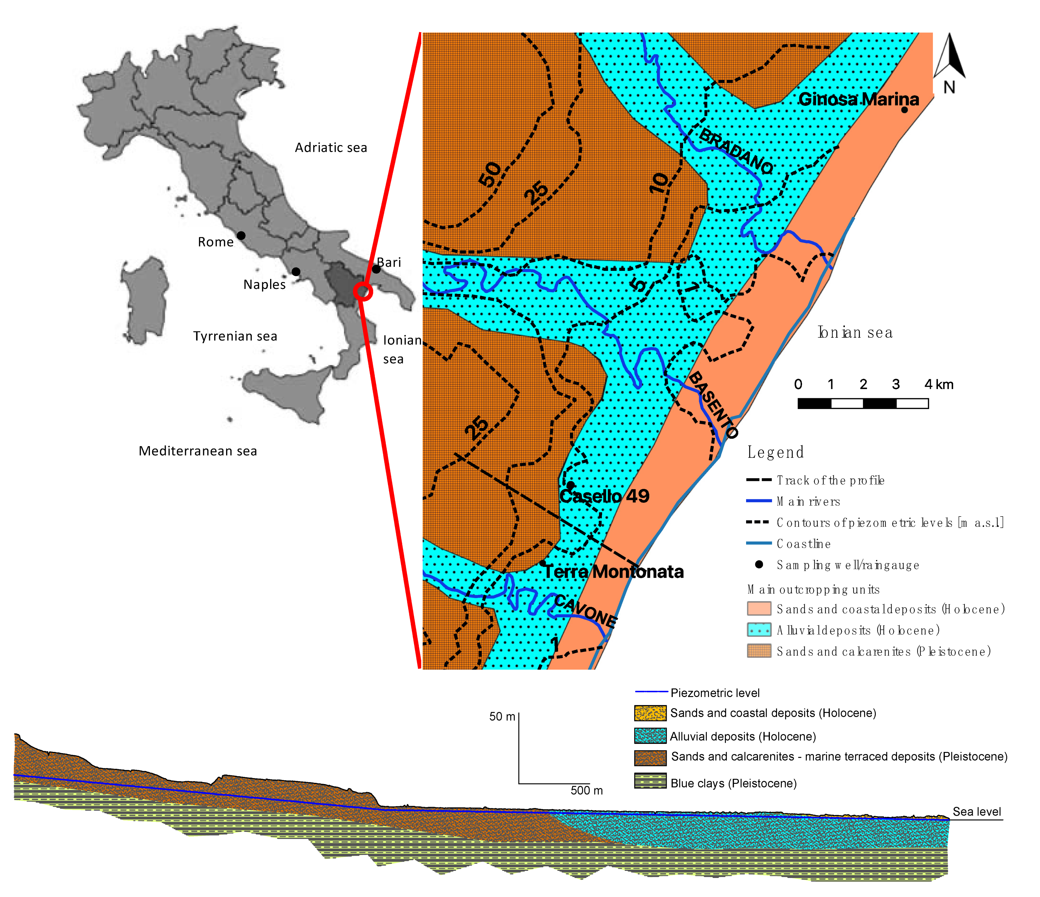
The shallow porous aquifer located on the coast of the Metaponto plain, in south Italy, is investigated here. This is a relatively extended aquifer, about 400 km
2, 40 km along the coast and averagely 10 km back towards the inland. It is located in the flat area between the valleys of the river Bradano, north-east, and river Sinni, south-west (see
Figure 1).
Its recharge comes from the backward terraced marine deposits, while locally there is a contribution coming from the presence of reclamation channels [
5,
21,
22]. The network of reclamation channels is organized as a matrix of channels, spaced about 100 m from each other. These are shallow artificial channels originally design to drain shallow backwater of the large coastal swamp. However, because of the increasing presence of structures and infrastructures, channels became drains for runoff coming from roads and roofs. As these channels are unlined, when they drain runoff, they can release part of the water into the shallow aquifer. Rivers do not contribute to the aquifer, as their beds are at an elevation that is lower than the bottom of the aquifer [
21,
23].
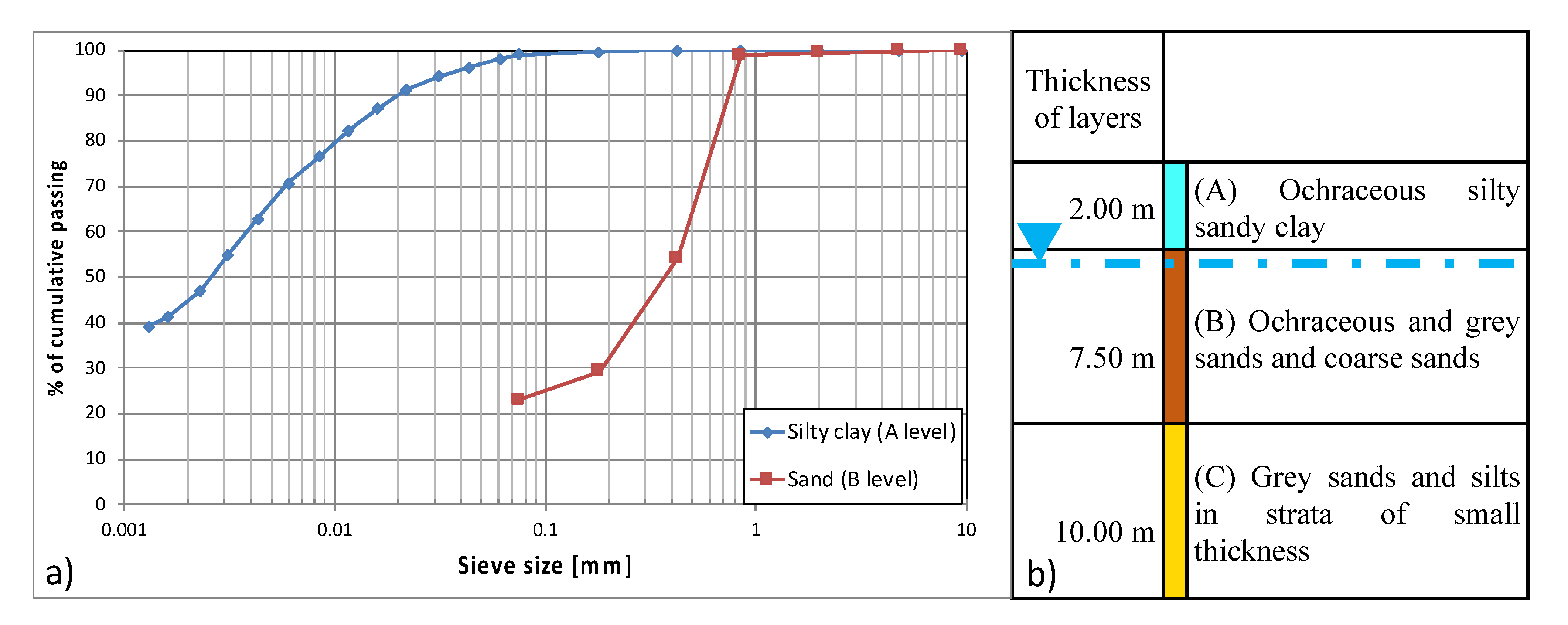
Close to the coast, the aquifer is hosted by the Holocenic alluvial sediments, constituted by fine grey sandy and silty layers with a small thickness (level C), with overlying ochraceous and grey sands and coarse sands (level B). The upper layer is made of ochraceous silty clayey (level A) and finally there is a thin, 30 cm at most, top soil layer (see
Figure 2). The aquifer develops upstream through the Pleistocenic terraced marine deposits, mostly constituted by sands and calcarenites [
5,
21] (see
Figure 1).
In the coastal area, groundwater flows through the level B, which is the aquifer level, characterized by the average value of hydraulic conductivity equal to 2 × 10
−6 m/s, with lower values in the order of 10
−6 m/s and upper values of 10
−3 m/s. Locally, the hydraulic conductivity can be even lower, with values ranging between 10
−7 to 10
−5 m/s; in particular, these values are measured close to the river valleys and approaching to the coast line [
21]. The shallow ochraceous silty sandy clay level A works as an aquiclude, as well as the blue clays at the bottom of the alluvial deposits (see the profile in
Figure 1).
The distribution of the hydraulic permeability is likely related to the irregular distribution of the silty clayey strata hosting the aquifer. Moreover, the presence of clayey levels forces the groundwater to flow at different levels, even if these levels are interconnected. It is noteworthy that the presence of level A, overlying the layer where the groundwater normally flows, works as an almost impermeable layer. Therefore, when the level of the groundwater exceeds the interface between level A and B, it starts flowing in pressurized conditions, thus changing the response of the piezometric height to the recharge.
Another variable is the presence of reclamation channels, which interact with the shallow aquifer, in general locally draining runoff and also fostering infiltration processes into the shallow aquifer.
Nearby the sampling wells, the water table is about 2 m deep in the ground. Rainfall directly recharges the backward heteropic terraced sand gravel aquifer, which is highly permeable and supplies the aquifer of the plain [
5,
21]. This implies that rainfall indirectly recharges the aquifer through quite quick flow paths.
3. Modelled Data: The Shallow Aquifer of Metaponto
In order to model the aquifer of Metaponto, here, the total monthly rainfall heights and the monthly average piezometric heads of the aquifer are considered. In particular, the monitoring periods of the aquifer correspond to the following two time windows: January 1951 to December 1975 and October 2001 to October 2018. After December 1975, the old network of sampling wells was discontinued and a new network was implemented in 2001; no data are available during the time gap. The sampling well used during the earlier time period is different from that used in the latter period, this one being located 2.5 km SW far from the previous well (see
Figure 1). These two wells are obviously drilled in the same aquifer and the water table is at approximately the same piezometric height in both wells, and the stratigraphic sequence is also the same; therefore, they are supposed to be closely correlated.
The Piezometric levels are available as single manual measures of the levels every three days in the time window of 1951 to 1975 and as automatic logged data with a sampling frequency of 1 level every 20 min in the time window 2001 to 2018. However, for both of the wells, given the structure of the aquifer and its non-local recharge, it was preferred to use the average monthly levels estimated on the available measures. This assumption is supposed to filter accidental errors of single measures as well as very short-term oscillations of piezometric levels not related to the recharge of the aquifer [
1,
20]. Similarly, for rainfall, two timeseries of total daily precipitations are available for both the monitoring periods of the aquifer. Rainfall data are collected by the same rain gauge for both of the sampling periods of the water table. The rain gauge is located in Ginosa Marina, a town located 15 km NE, along the coast. This particular station is representative of the climate and of the rains occurring on the recharge zone of the aquifer, as well as possessing a long uninterrupted timeseries of daily data since 1927. This rain gauge station is part of the monitoring network managed by Regione Puglia; data are available at
http://93.57.89.4:8081/temporeale/meteo/stazioni, accessed on 6 July 2021.
In this case, the total monthly value of rainfall was considered and was used as the input, i.e., forcing variable, representative of the recharge of the aquifer. In this way, two timeseries, i.e., average monthly piezometric levels and total monthly precipitations, were generated, each made of 300 values.
The sampling well, named “casello 49”, used in the period 1951–1975, is located at the low elevation area of the aquifer, 3.1 km from the coastline, on the side of a railway line in a rural area. Its timeseries is constituted by 25 years of measures of the piezometric level, measured every three days. Data are available as a scanned PDF of the original paper documents, through the website of the Higher Institute for Environmental Protection, Istituto Superiore per la Protezione dell’Ambiente e la Ricerca Ambientale, ISPRA, at
http://www.acq.isprambiente.it/annalipdf/, accessed on 6 July 2021.
The sampling well was exclusively used for sampling purposes—no pumps are installed and there are no pumping wells in the neighborhood of the well.
The sampling well, named “Terra Montonata”, is located 2.5 km SW far from “Casello 49”, in a rural area. It is 2.5 km from the coastline and, differently from the “Casello 49”, it has an automatic data logger, which is part of a real time monitoring network managed by Regione Basilicata and is available at
http://www.centrofunzionalebasilicata.it/it/, accessed on 6 July 2021. It has a timeseries of 18 years of data, available as piezometric levels sampled every 20 min. No pumping activities are known close to the well.
Table 1 provides some details and statistics about the rain gauge and sampling wells. These are referred to as monthly data, which are used for the following modelling stage.
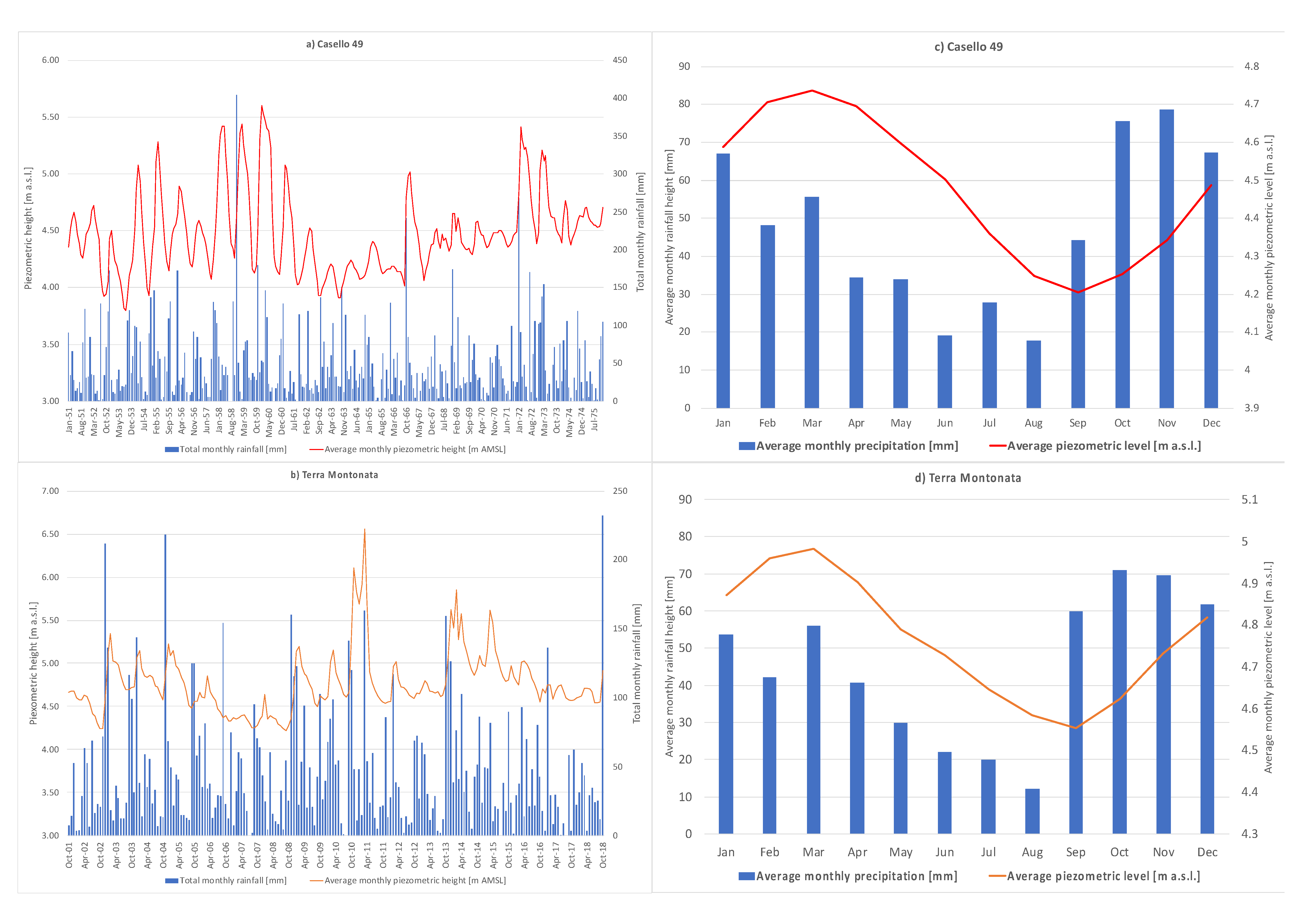
Figure 3a,b shows the time plot of the timeseries of the rainfall and piezometric levels, while
Figure 3c,d represents the average monthly values for the sampling windows of each well. Looking at the piezometric data, it is possible to observe that water table peak values follow rainfall peaks. In particular, piezometric peaks lagged by about 1–2 months with respect to precipitation, which is consistent with the structure of the aquifer and with the assumed recharge.
Looking at the piezometric data, the highest values for the depth of groundwater are very low for both wells. In addition, the oscillation band of piezometric data is of 2 m for both the wells, with a similar average value for both wells. Given the geological nature of the top-soil, mainly constituted by silty-clay deposits, this can imply occasional pressurized flow through the aquifer, at high groundwater levels, which can affect the hydraulics of the aquifer and the headlosses related to the flow of water. In fact, when groundwater flows under pressure, it can create a quick increase in the piezometric level, without a severe increase in the amount of water in the aquifer. Finally, looking at the data of Casello 49, starting since 1967, groundwater levels show a moderate increasing trend up to the end of the observed data, likely related to the presence of an unknown extra-input, which is possibly related to uncontrolled irrigation.
4. The Modelling Approaches
The response of the average monthly groundwater levels to the total monthly precipitations are modelled here according to two methods: multi-objective evolutionary polynomial regression (EPRMOGA) and recursive artificial neural networks (NNARX). For both the approaches, the groundwater levels were scaled on the range 0 to 1, in order to have the same range of variability for both of the sampling wells.
4.1. EPRMOGA
EPRMOGA is a data-driven machine learning paradigm that automatically identifies and optimizes models [
19], returning explicit closed-form equations. It works according to a two-stage approach: the structures of the equations are identified using a genetic algorithm [
24,
25], and then, an estimation of the constant values is made based on a least-square approach. EPRMOGA optimizes the polynomial structures and their coefficients in order to fit data, as well as keeping the structural complexity of the equations relatively simple. The evolution is based on the contemporary minimization of three conflicting objective functions. These are the sum of squared residual errors (SSE), the dimension of the polynomials, and the selected input variables among the pool of candidates assumed by the user. The outcome of this multi-objective optimization is a set of solutions, representing a Pareto set [
26], which can be used for comparing the equations, and making a robust choice of the model. The main benefit of EPRMOGA is that the models are explicit polynomial equations, which allow for some speculations on the relationship between the main variables of the investigated phenomena.
The terms of the equation can represent either the measured values of rainfall or measured values of the past piezometric head. Past measured piezometric heads constitute the stochastic component, related to extra input or to non-Gaussian errors [
27], representing the state of the aquifer, containing all of those inputs not directly related to rainfall.
In order to let EPRMOGA identify the models of the response of water levels to rainfall, the timeseries sampled from Casello 49 is used as the training set, while the timeseries from Terra Montonata is used as the testing set. Here, the testing set in meant as a set of data that are not used during the learning phase. This subdivision is supposed to test the generalization capabilities of the returned models.
The following candidate variables are used: Ht−1 and Ht−2, representing the monthly piezometric heads, one and two months before the output, respectively. and Pt, Pt−1, Pt−2, Pt−3, Pt−4, Pt−5, and Pt−6, corresponding to the total monthly rainfall height of the last 6 months preceding the output. The choice of these candidate variables allows for accounting for both rapid (e.g., Pt) and slow (e.g., Pt-6) infiltration processes, which can recharge the superficial aquifer of Metaponto.
The set of exponents of the variables of the polynomials are assumed, limited to 0, 0.5, 1, and 2, while the maximum length of the polynomial structures is set to four terms. This should limit the complexity of the search space, enhancing the efficiency of the genetic optimization. Moreover, the limitation of the complexity boosts EPRMOGA to find equations, which can be physically sound. The choice of exponents depends on some simple practical reasons: the exponent 0 allows for unselecting a variable during the search, while the other exponents are related to an attenuation effect (square root), a linear dependence (1), and an amplification effect on the variable (square).
Not all of the variables will be necessarily represented in the models, as each model is the result of a structural optimization, which is aimed at keeping the structure of the model parsimonious, as well as at the maximization of the model fitting of the measured training data. Equation (1) represents a very general expression of the structure of equations optimized by EPRMOGA:
where
Xk is the vectors of candidate inputs;
H is the model-returned piezometric level
ES is the matrix of exponents;
aj is the constant parameters; and
m is the length of the returned expressions, i.e., the number of terms of the polynomial structure returned by EPRMOGA. The constant parameters,
aj, are estimated by a least squares approach integrated in EPRMOGA.
The fitting of predictions based on the EPRMOGA models is evaluated in terms of Nash−Sutcliffe efficiency (NS) [
28]:
where
is the value of the i-th water table level returned by EPRMOGA,
Hi exp is the i-th measured value of the water table height,
N is the numerosity of the set of samples, and
avg(H) is the average value of the measured heights. In particular,
NS is a performance indicator in terms of the goodness of fit of the model-retuned data to the measured data. This efficiency, i.e., the fitness, is maximum when
NS is 1. It is also interesting to observe that
NS is a non-linear indicator; therefore, when it approaches 1, a very high improvement of the fitness is necessary in order to have a slight increase of
NS. Finally, low values of
NS, i.e., values lower of equal to 0, mean that the sum of the square errors exceed the variance of the measured data.
A further performance indicator considered here is the value of the variance of residual errors (VAR). It is a statistical indicator of the quality of fitness and of the distribution of the residuals; the lower the variance, the better its fitness.
Finally, EPRMOGA performs uncertainty analyses on models and on the performance indicator of data fitting. As described by Giustolisi and Savic [
19], EPRMOGA makes an estimation of the uncertainty of each term of models based on the asymptotic covariance method [
27].
4.2. NNARX
Recursive neural networks are powerful non-linear learners based on highly connected networks, which reproduce the neural system, well known by scientific literature and broadly used for practical applications [
13,
14,
29]. Based on the knowledge of the brain and its associated neural systems, ANNs use highly simplified models composed of many processing elements, neurons, connected by links of variable weights, parameters, to form a black-box representation of systems [
18]. These models have the ability to deal with a large amount of information and to learn complex model functions from examples, i.e., by training sets of input and output data. The greatest advantage of ANN over other modelling techniques is their capability to model complex, non-linear processes without assuming the form of the relationship between the input and output variables. Learning in ANN involves tuning the parameters, i.e., weights, of interconnections in a highly parameterized system. However, differently from EPRMOGA, an ANN requires that the structure of the neural network is identified a priori, e.g., number of inputs, kernel type, transfer functions, and number of hidden layers. ANNs have been successfully used on manifold case studies related to the prediction of groundwater levels. For instance, Giustolisi and Simeone [
16] successfully attempted the use of optimized recurrent ANNs for the prediction of the response of piezometric levels of groundwater to the precipitations, in a climatic scenario and on a porous aquifer, where boundary conditions were relatively stable.
Similarly to EPRMOGA, here, ANNs are used according to a recurrent scheme, NNARX, i.e., past measured values of the piezometric levels are used as the input for the network. The complexity of the architecture of the NNARX is intentionally kept relatively simple; in particular, the general architecture of the network is made using an input layer, hidden layer, and output layer. It is assumed the use of three precipitation inputs, corresponding to the precipitations of the same months of the output and of one and two months before. In addition, one past measured value of the piezometric head is used as the recursive input, while the hidden layer is made of five neurons. A number of networks are trained, the choice of the sub-optimal network is made according to the criterion of maximizing the fitting of the predicted values on the testing set of data, i.e., not used for training the network. The training is based on the Levenberg−Marquardt backpropagation algorithm [
30]. Finally, the kernel function of the NNARX is assumed to be the hyperbolic tangent, which seems to return better performances than the other kernel functions tried on this specific case study, keeping the same architecture of the network.
The performances of NNARX are evaluated in terms of the VAR and NS coefficient, similarly to EPRMOGA, in order to have a quick comparison between the EPRMOGA and NNARX results.
5. Modeling Results
EPRMOGA returned a Pareto set of 11 equations, representing the models of the piezometric level responses to precipitations. These equations show relatively simple explicit structures, even if non-linear, able to predict piezometric levels. The list of equations follows, ordered from the simplest one, which is the mean value of the scaled piezometric value, to the most complex on the Pareto front.
The returned models are the outcome of the optimization of three conflicting objective functions; therefore, none on them can be considered as absolutely the best.
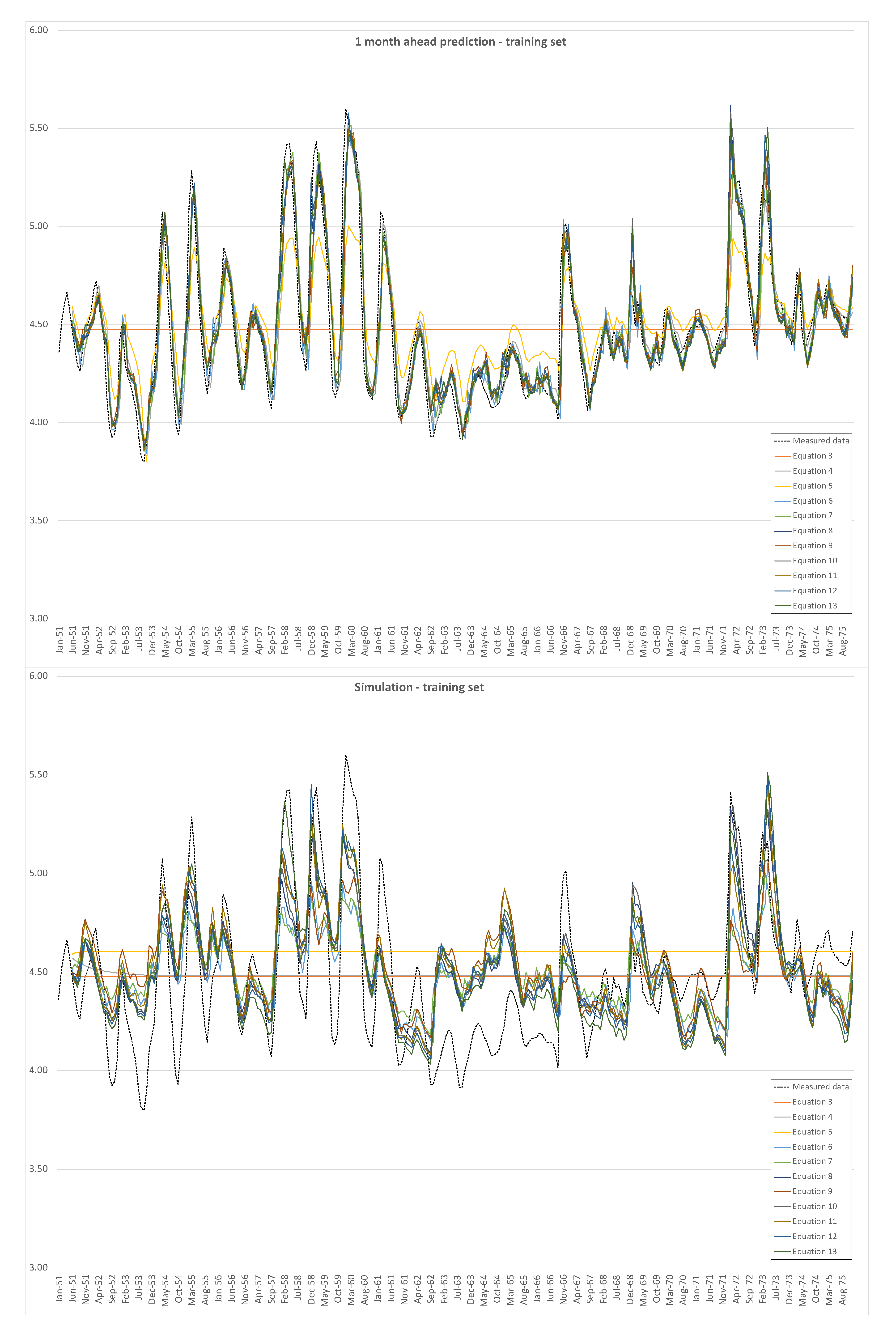
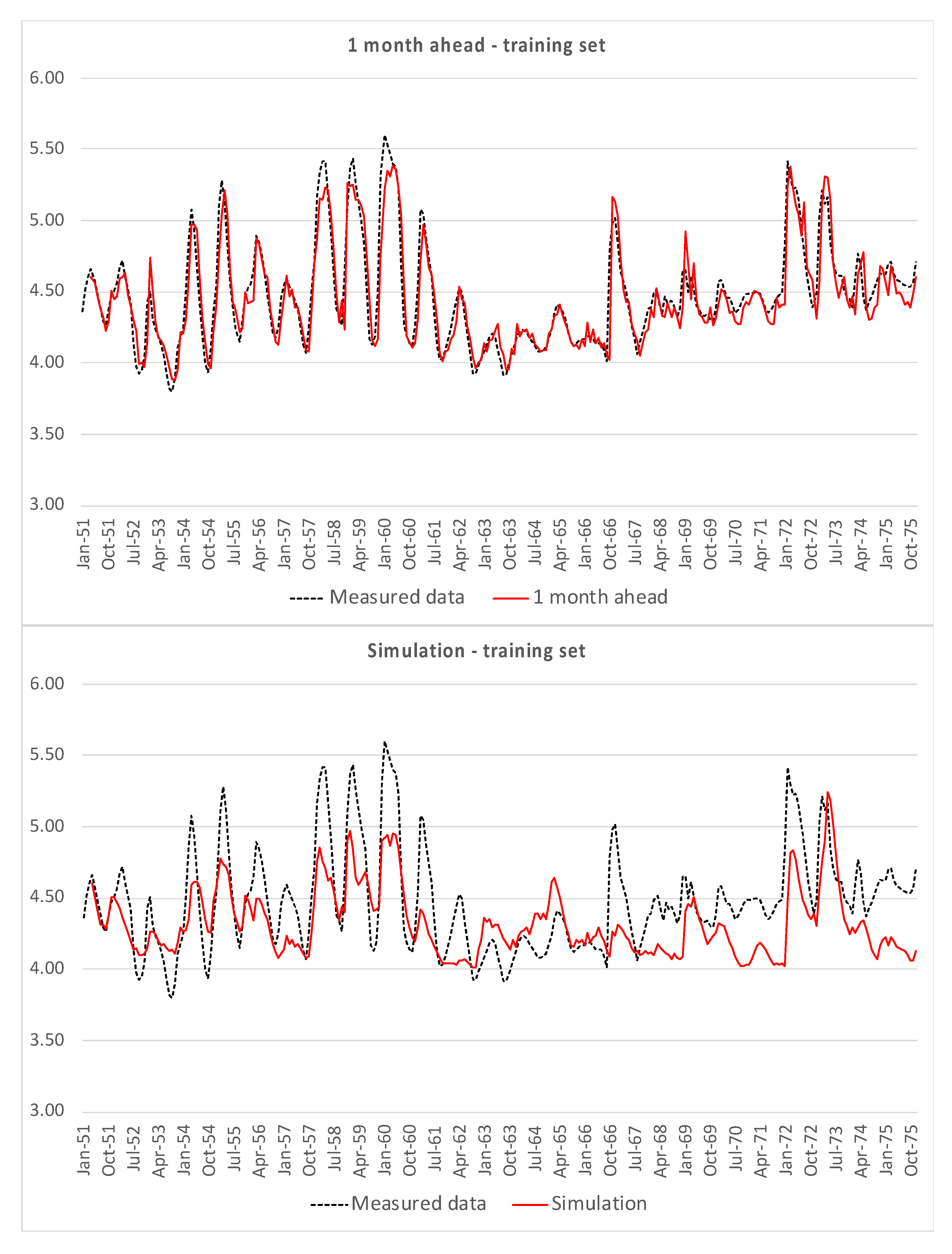
Figure 4 shows the one month-ahead predictions and the time plot of simulations, both compared with the measured data, for the training set, i.e., data from Casello 49.
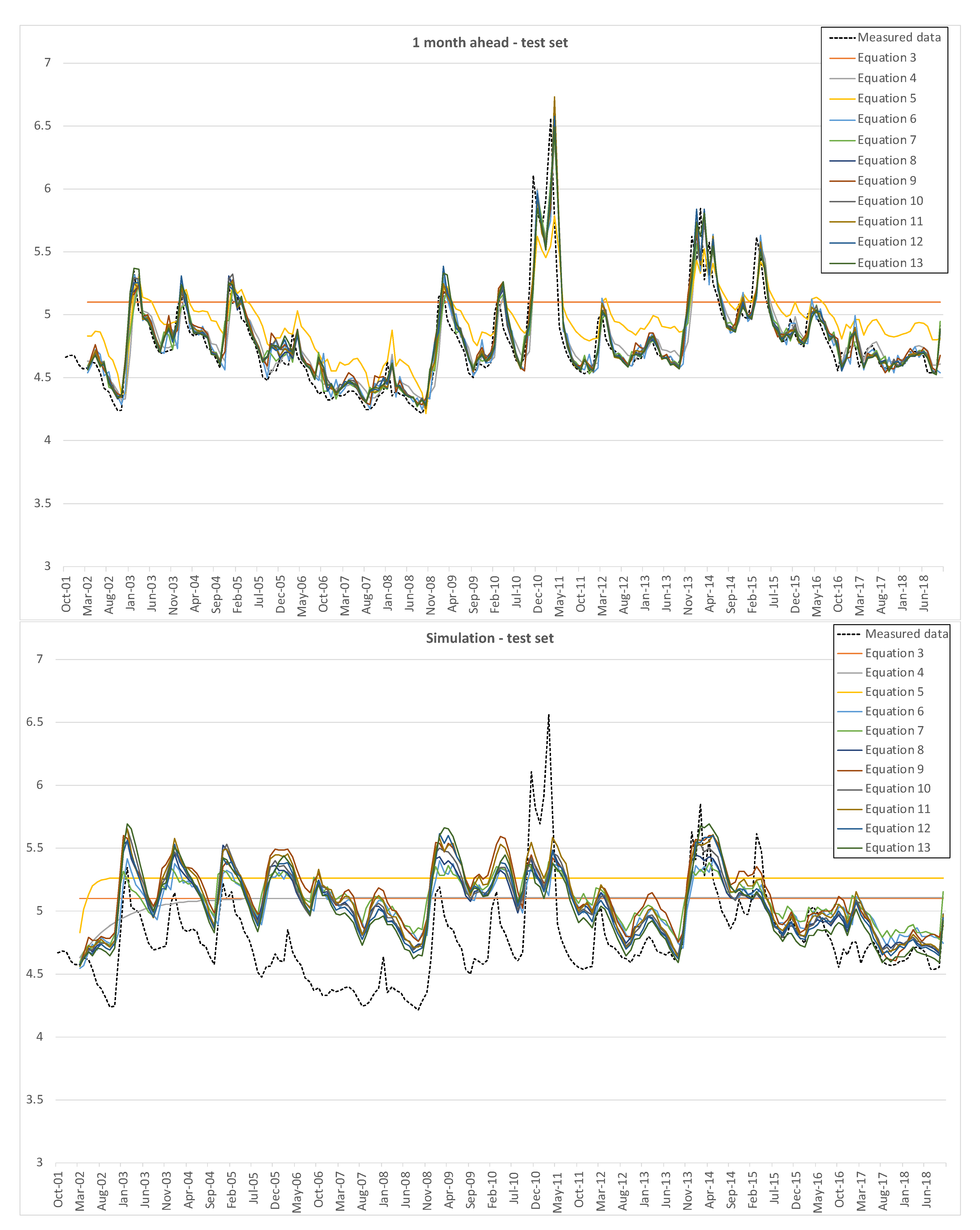
Similarly,
Figure 5 represents one month ahead predictions and simulations for the test set, i.e., data from Terra Montonata.
Both for the training set and for the test set, the one month ahead prediction is quite consistent with measured data, except for the simplest model (3). The hard test is constituted by the simulations, which do not show good results, in particular for peaks and minima.
Table 2 and
Table 3 show the performance indicators of training and test sets, respectively, for the one month ahead predictions and simulations, in terms of VAR and
NS values.
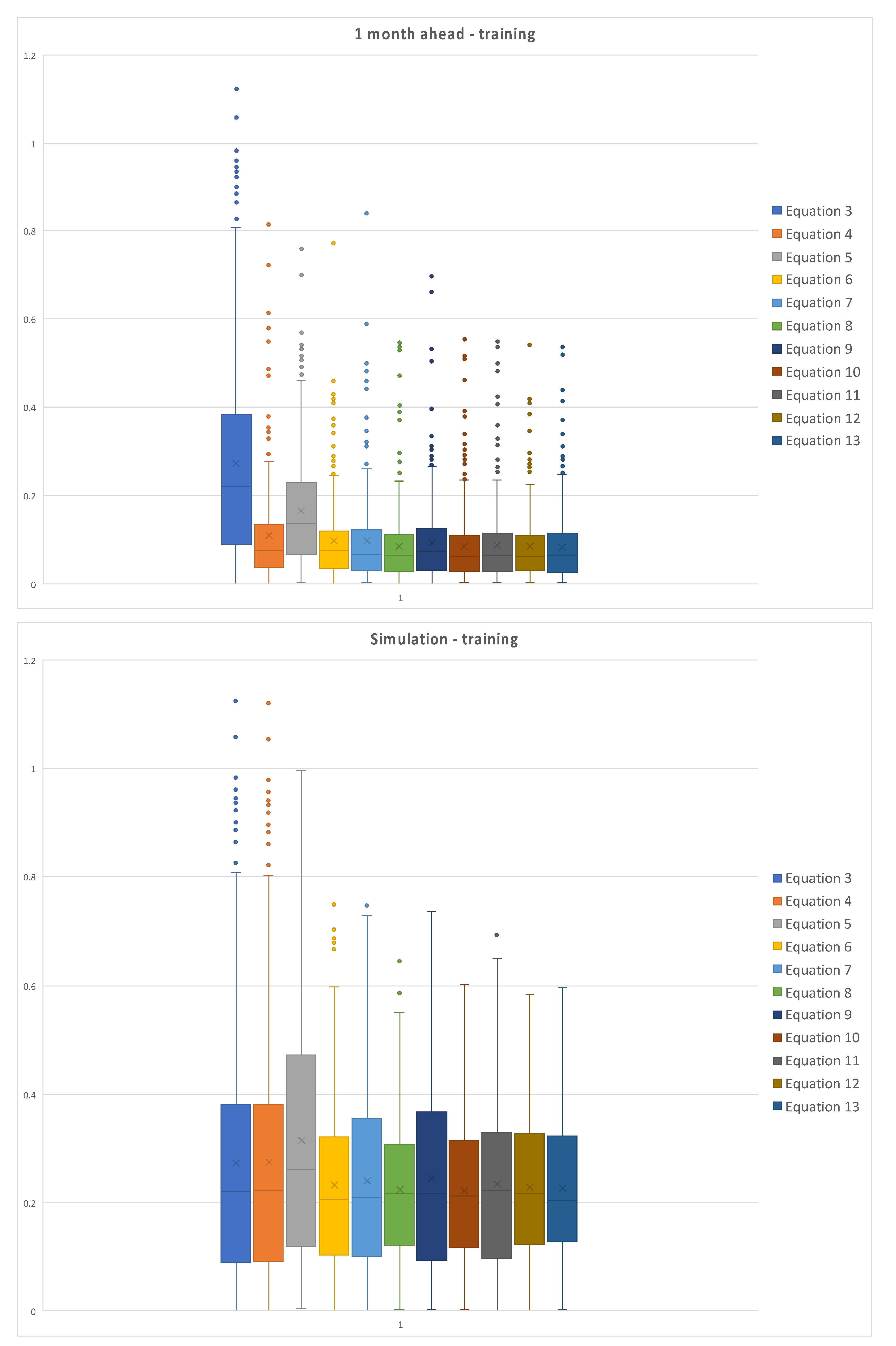
Figure 6 represents the box plot of the absolute values of the errors for the training set of data, for each model, with the one month ahead prediction on the left and simulation on the right.
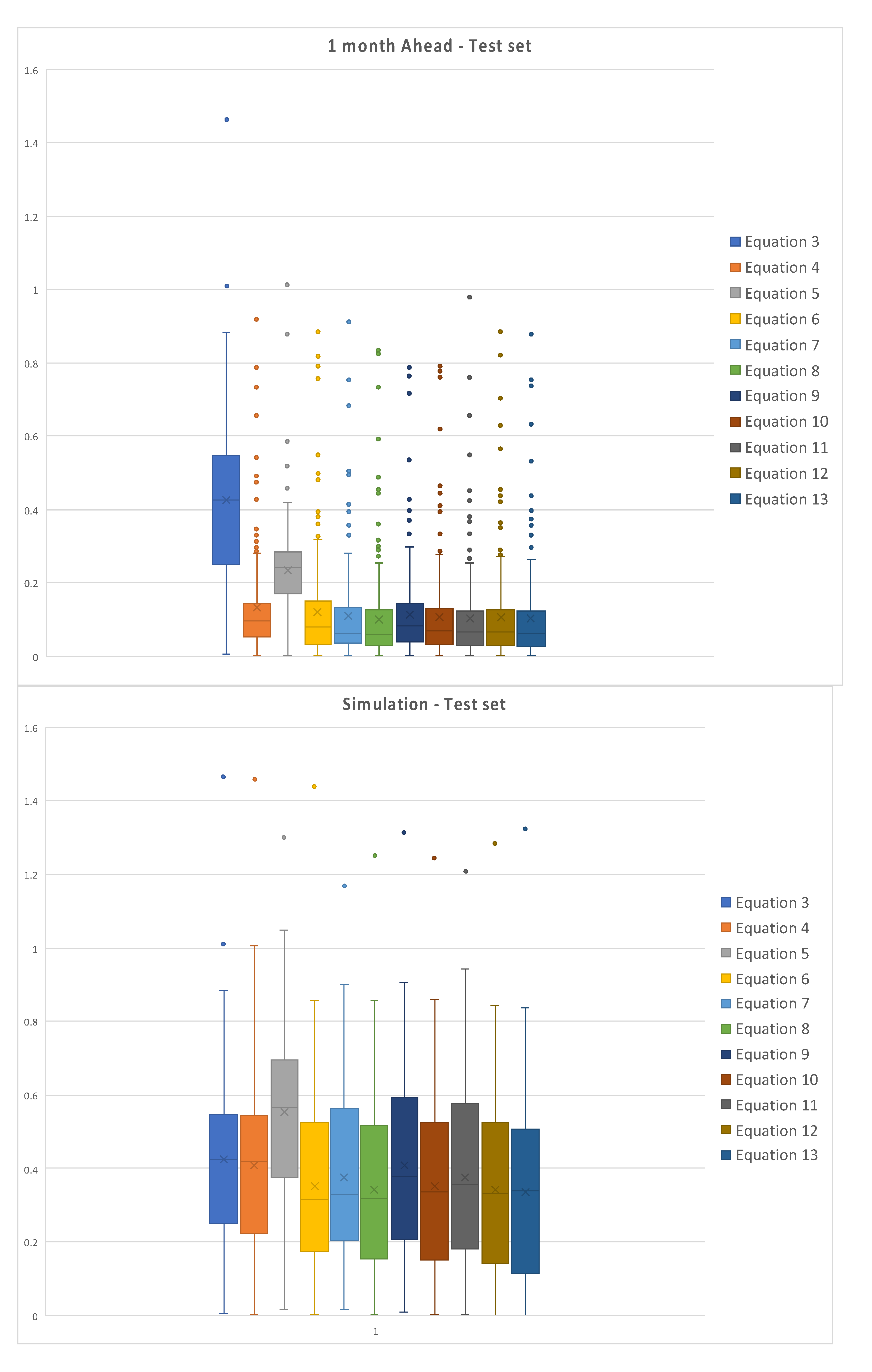
Similarly,
Figure 7 represents the box plot of the absolute values of the errors for the test set of data, for each model, for the one month ahead prediction on the left and simulation on the right.
It is possible to observe the dispersion of the errors for simulations, both for training and test set; errors for the one month ahead are relatively less dispersed, due to the better fitting of model returned data to measured ones. Moreover, simulations are characterized by higher uncertainty, since it is conditioned by the fails in reproducing peaks and minima, while the mid-range oscillations are relatively well simulated.
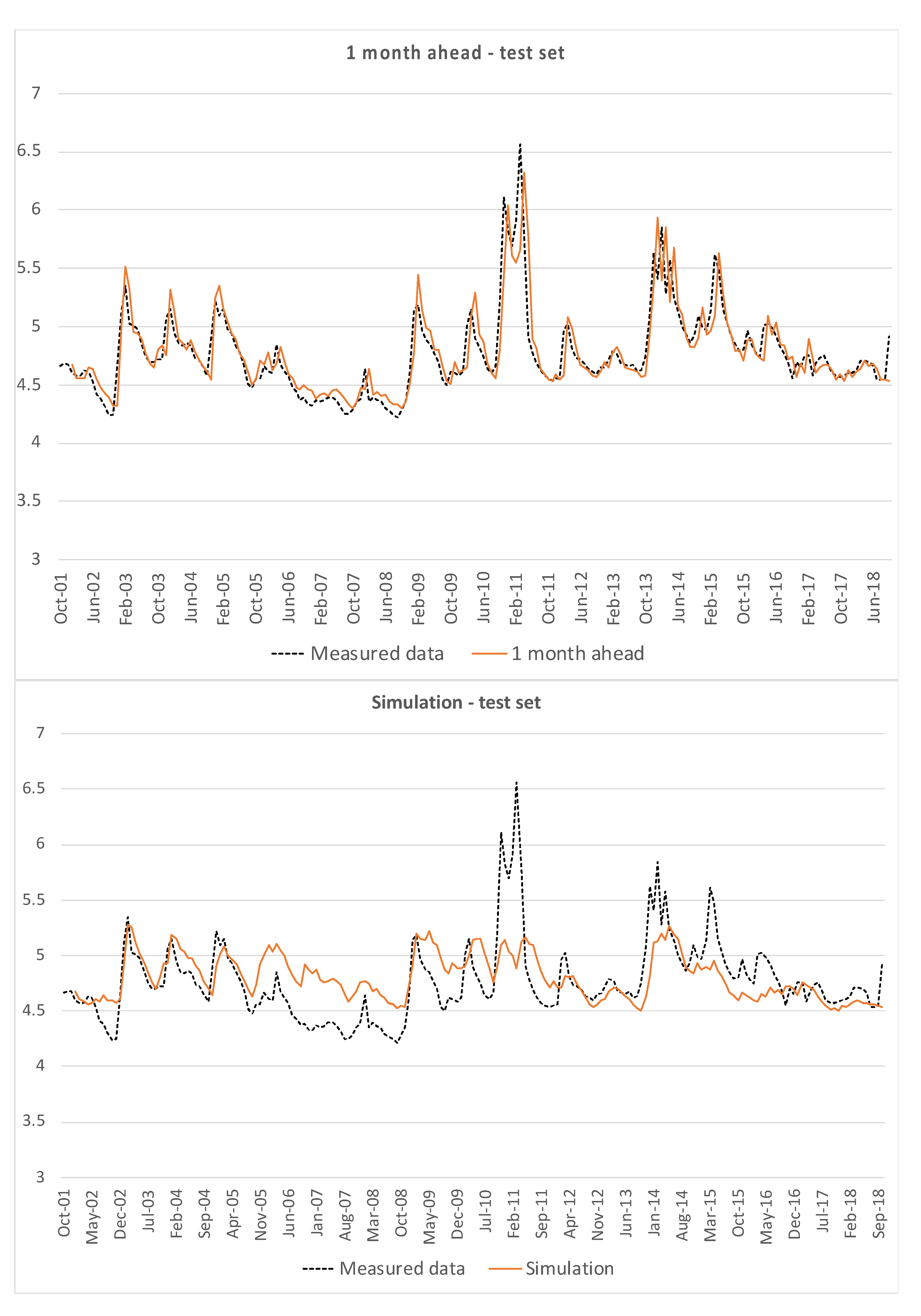
NNARX based model shows slightly better results, in particular for simulation. However, even in this case, peaks and minima are not simulated. The next
Figure 8 and
Figure 9 represent the one month ahead prediction and simulation in the order for the training and testing set.
Table 4 reports VAR and NS for the one month ahead prediction and simulation for the training and testing set.
Finally, it is interesting to emphasize that both EPRMOGA and NNARX contain the recursive term of the piezometric level measured the month before the prediction. This term, representing the stochastic component, contains the information not related to the rainfall. Therefore, the effects of the reclamation channels are modeled by this term, together with all of the other extra input and non-Gaussian errors.
6. Discussion on Results
The presented models are directly learned from the measured data, from which they learned the responses of the groundwater piezometric levels to precipitations. However, for both EPRMOGA and NNARX, it is possible to observe that these two different paradigms were able to learn the responses of the groundwater levels to he precipitations in the mid-range of groundwater levels. In general, the oscillations of the groundwater levels are somehow fitted by the simulations returned by EPRMOGA and NNARX.
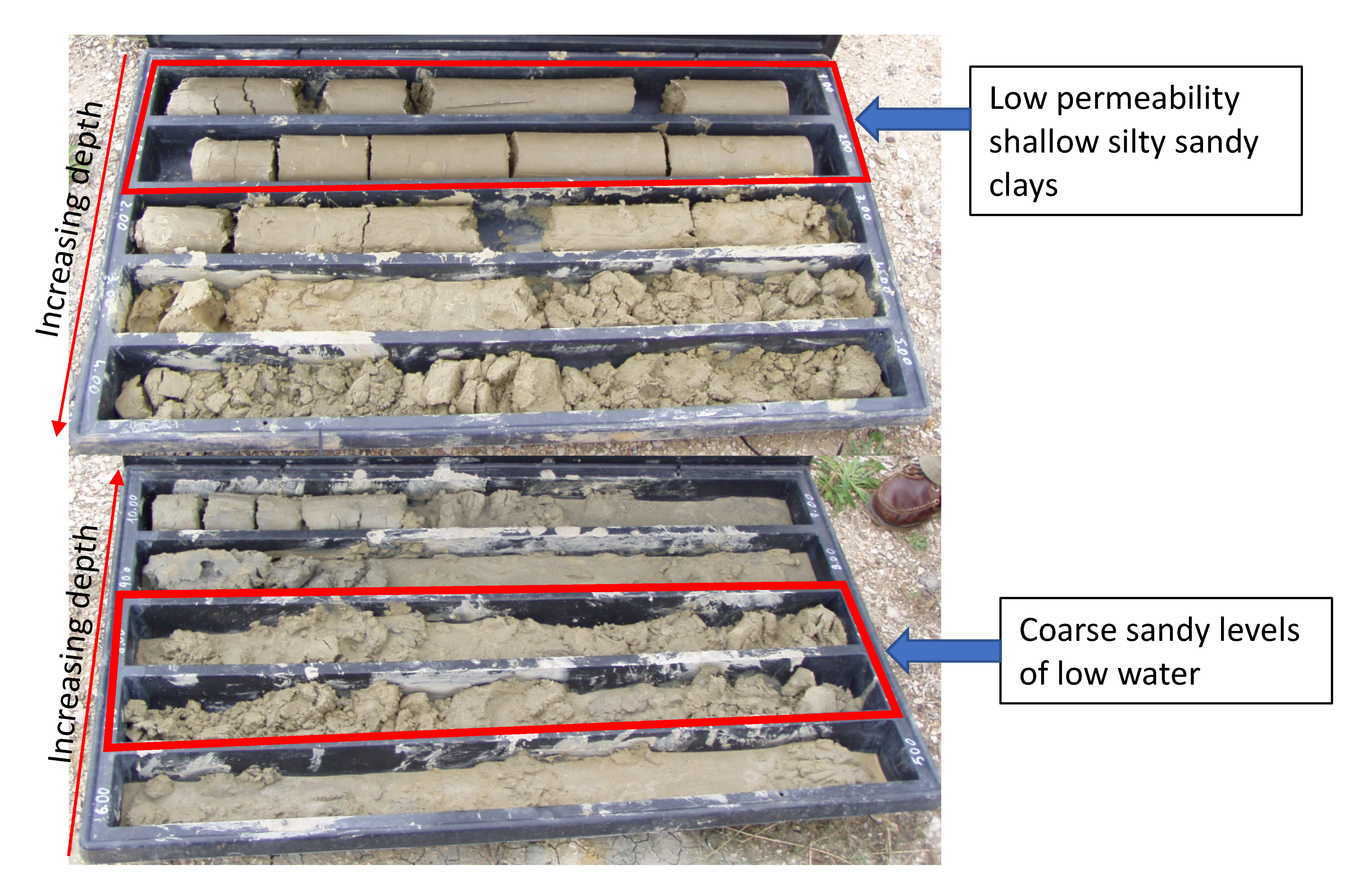
The peaks and minima are not predicted, in particular for simulations, when models are completely recursive, i.e., except for the initial conditions, the component of the past measured groundwater levels are recursively generated by the models. Therefore, simulations test the ability of the models to reproduce groundwater levels without using the stochastic component given by the past measured levels. This component is supposed to contain the information not related to the rainfall precipitations, but to other unknown variables or to non-gaussian errors. In this particular case, the unknown variable is the variation of the boundary conditions. Indeed, the investigated aquifer normally flows in a layer made of grey sands and coarse sands; this layer is comprised between two low permeability silty layers on the bed and on the top. The upper silty-clayey level works as a confining layer; therefore, when the groundwater level exceeds the elevation of the interface between sands and silty-clayey sands, the aquifer flows under pressure [
5]. This pressurization generates a sudden increase in the piezometric level, which constitutes an anomaly that rarely occurs; therefore, both EPRMOGA and NNARX are not able to learn these anomalies. This is the reason both methods fail at simulating the peaks. The minima are also not simulated, in this case the motivation can be related to the vertical anisotropy of the coarse sandy level. In fact, the lower levels of sands are interlayered by coarse loose sands and gravel, which have a higher storage coefficient. Therefore, when the groundwater level decreases and encounters these coarse loose sand, it suddenly decreases, causing the measured minimum values. Therefore, the minima of the groundwater levels are again anomalous, as the lowering of the levels is sudden and is not correlated with the flow of the aquifer through the sandy layer. This peculiar behavior of the aquifer was proven using a physically-based model by Pastore et al. [
5], and the machine learning approaches presented here are consistent with those results, even if independently obtained.
Figure 10 shows the shallow low permeability layer and the coarse sand layer for a borehole survey made close to Terra Montonata well. Unfortunately, the borehole was drilled for purposes not related to this research, and thus no other information is available.
These exceptional occurrences imply that both the paradigms do not learn these unpredictable variations of levels, as they are poorly correlated with the variations of the levels observed in the sandy layer. Therefore, the combination of the low-permeable layer at the top and of the presence of interlayers of coarse loose sand generate the characteristic scenario with anomalous peaks and minima of groundwater levels. It is noteworthy that in the mid-range of levels, both EPRMOGA and NNARX are able to accurately predict and simulate the oscillations of the groundwater piezometric levels as a response to precipitations. In fact, the mid-range of the levels represent the oscillations of the aquifer in the coarse sandy level, and thus a sort of ordinary scenario.
It is also of interest to observe the structures of the models returned by EPRMOGA. Most of the identified models contain rainfall terms of the same month of the level to be predicted or of the month before at most. This means that the response of the aquifer to precipitations is relatively quick; however, this seems to contradict the presence of the poorly permeable layer on the top of the coarse sand. However, this relative quick recharge may be correlated to two reasons, namely: the presence of a number of artificial channels in the remediation system and the non-local recharge. Artificial channels are designed to drain backwater, avoiding the generation of swamps and ponded areas. However, because of the urbanization of the area, they drain runoff from waterproof surfaces. Therefore, they may directly interact with the shallow aquifer, and in particular with the coarse sandy layer, favoring the recharge of the aquifer, creating a relatively quick component of rainfall infiltration, also assumed by Pastore et al. [
5]. This hypothesis is not supported by numerical measures, which are not available, but it is plausible given the presence of a network of channels, structured as a matrix, with interrexes of 100 m.
The non-local recharge boosts the response of the aquifer to precipitation. Precipitation infiltrates through the regressive terraced marine deposits, constituted by sand and calcarenites outcropping backward from the area where the sampling wells are located and then it flows directly through the sand, without the hindrance of the silty-clayey top level. Therefore, even if EPRMOGA generally shows a slightly poorer fitness of predicted and simulated data than NNARX, it is useful as it returns explicit equations, which allow for some speculations about the component of the rainfall actually influencing the oscillations of the groundwater levels. Moreover, the explicit models returned by EPRMOGA allow for simulating possible scenarios of precipitations and then planning the use in terms of the pumping of groundwater.
NNARX is also useful, as it is a powerful method, but in this casem it failed at simulating peaks and levels, thus implying that those values were somehow poorly correlated with the larger part of the measured data. Therefore, the poor performances of NNARX in simulating the peaks and minima is consistent with the combined effect of the poorly permeable layer at the top and of the interlayers of coarse loose sands at the bottom of the sandy layer hosting the aquifer. These affect the oscillations of the levels when they go out of the mid-range band of levels.
7. Conclusions
The responses of monthly groundwater levels to the total monthly precipitations are investigated here by two machine learning approaches. The peculiar feature of the investigated aquifer is that it normally flows unconfined through a sandy layer interlayered by coarse loose sand, comprised between two low permeability silty-clayey layers. Moreover, the aquifer is recharged by the upstream area of its catchment, where coarse sands outcrop. The combination of these peculiarities, together with the presence of a network of reclamation channels, makes the boundary conditions of the aquifer complicated to model. In fact, when the aquifer exceed the upper bound between the sands and clayey sands, it starts working as a pressurized aquifer, with a sudden increase of piezometric levels. On the other hand, when the level of the aquifer is particularly low, it meets the coarse loose sand interlayers, characterized by higher storage coefficients. This implies a sudden decrease in groundwater levels. In addition, the recharge of the aquifer is affected by the presence of the network of remediation channels, which drain shallow water as well as facilitating the exchange of water between the sandy aquifer and the channels themselves. All of these factors make the modeling of the oscillations of the piezometric levels of the aquifer very complicated, as there are clearly different behaviors related to the ordinary levels, i.e., those corresponding to the unconfined flow of the aquifer with mid-range levels, and extraordinary conditions, related to the peaks and minima of levels. Here, two data-driven paradigms are used in order to let them learn the responses of piezometric levels of precipitation. The earlier is EPRMOGA, an optimized evolutionary modeling approach, able to return explicit equations, representative of the investigated phenomenon. These explicit equations can be used for predicting and simulating the responses of the piezometric level of the aquifer to precipitation. This permits for planning the use of groundwater, given precipitation scenarios of short- or long-term, by using relatively simple equations.
The latter is a recursive neural network, NNARX, which is a deep learner, able to return models with a high fitness to the measured data. This was here tested, in order to understand the real benefit over EPRMOGA for using a powerful black-box learner in terms of prediction and simulation.
For both the approaches, it was not possible to simulate the peaks and the minima, i.e., the extraordinary boundary conditions. On the one hand, NNARX slightly outperformed ERPMOGA in simulation; on the other hand, EPRMOGA, returning explicit equations, confirmed the role of the short-term precipitation for the recharge of the aquifer.
Therefore, even if data-driven paradigms seems to fail at simulating the oscillation of groundwater levels, they were actually useful for emphasizing the unpredictable oscillations when boundary conditions change. Particularly, EPRMOGA allowed for identifying which rainfall component is mostly influencial on the recharge of the aquifer. Finally, NNARX and EPRMOGA returned a model able to decently simulate the mid-range values of the piezometric heights, which corresponded to the phreatic behavior of the aquifer [
19].


