
Digital Elevation Models of Rockfalls and Landslides: A Review and Meta-Analysis


Abstract
1. Introduction
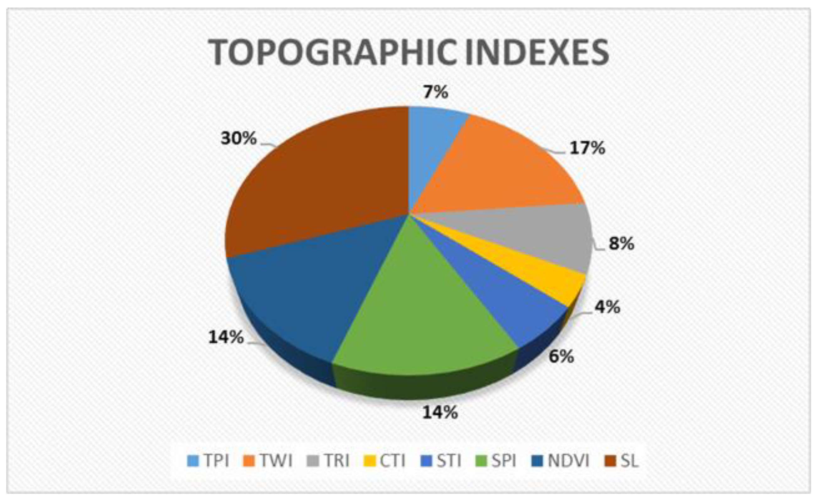
2. Topographic Indexes
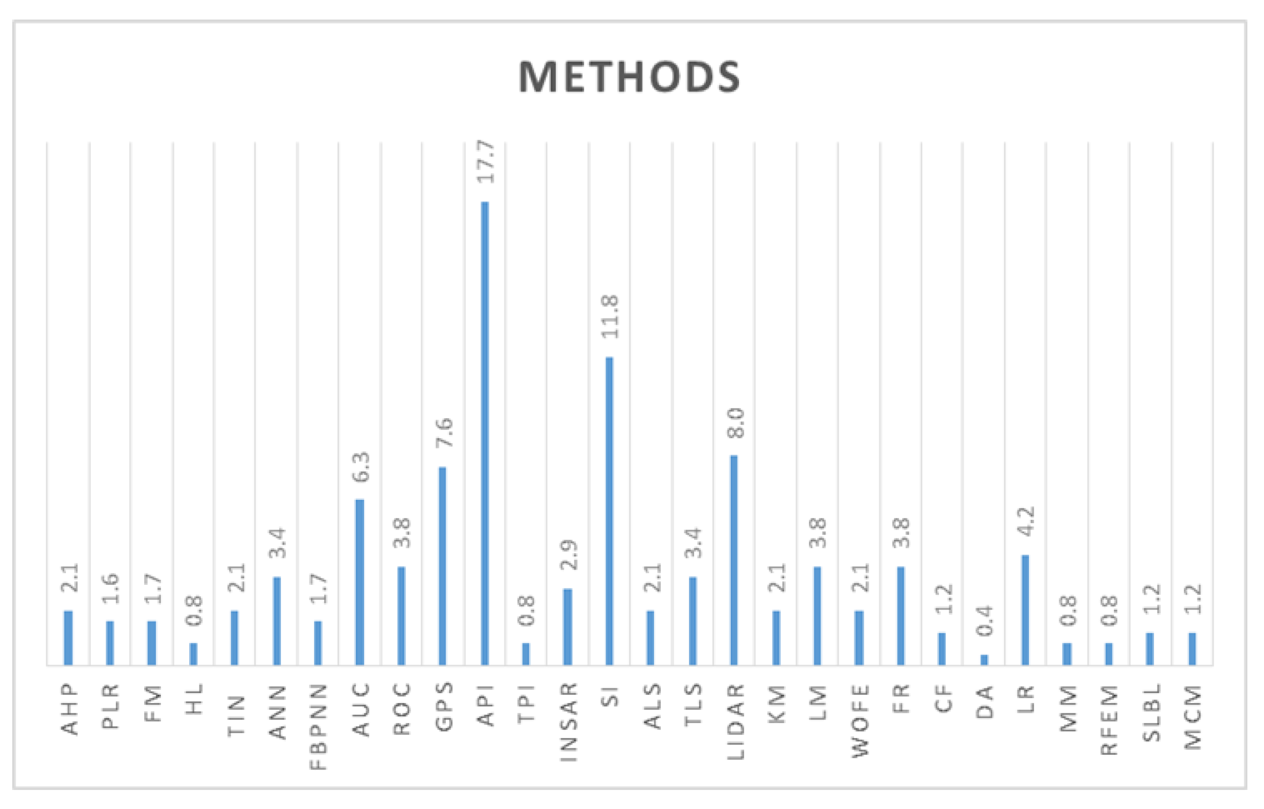
3. Methods
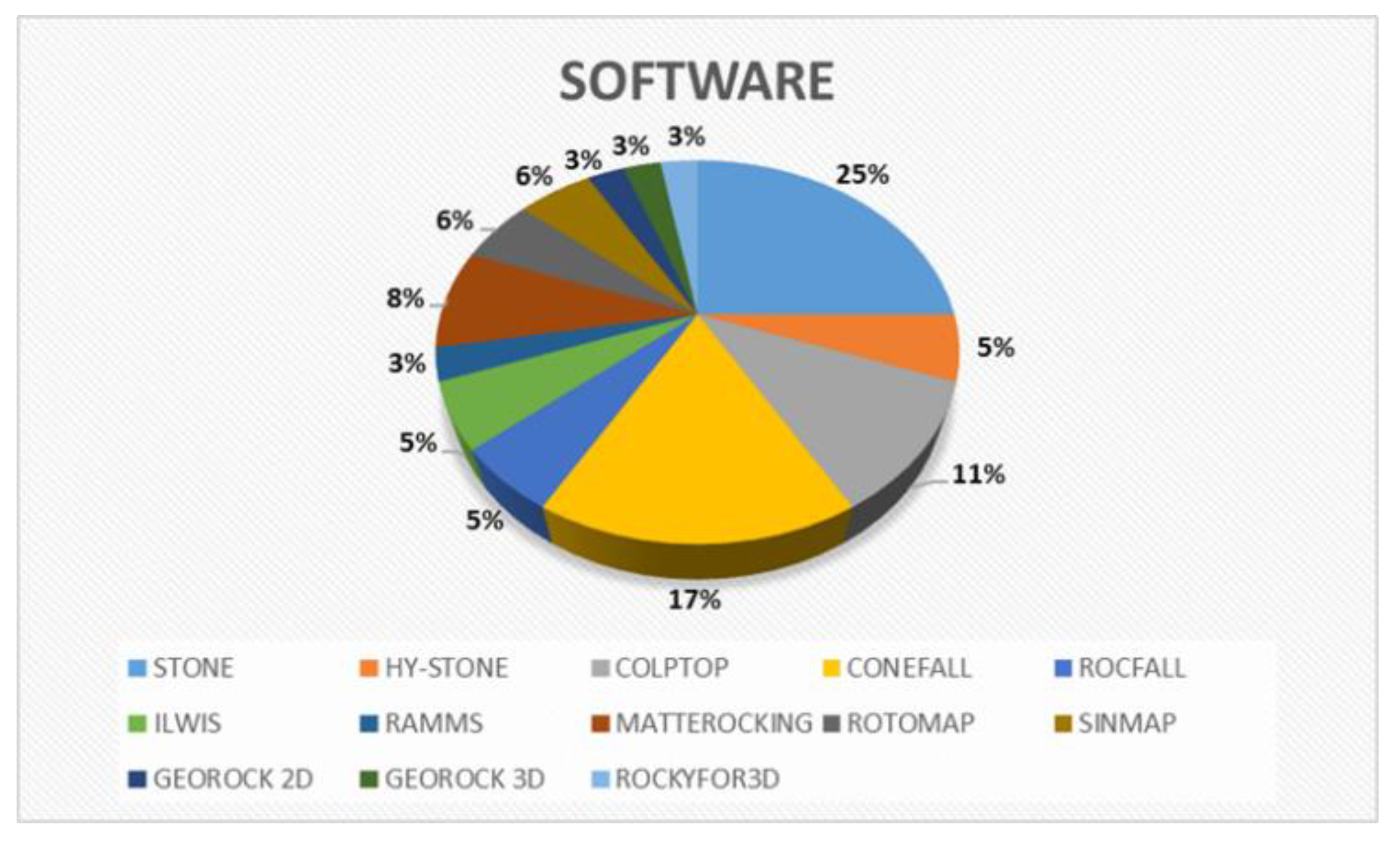
4. Software
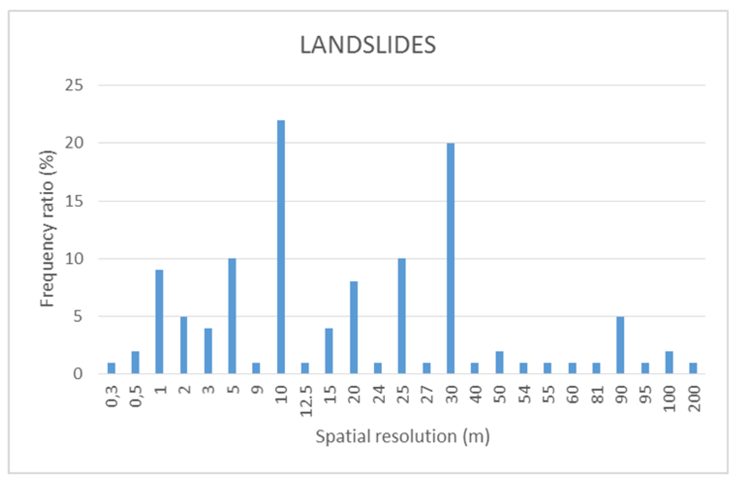
5. Spatial Resolution
5.1. The Effect of Digital Elevation Model (DEM) Resolution on Landslides
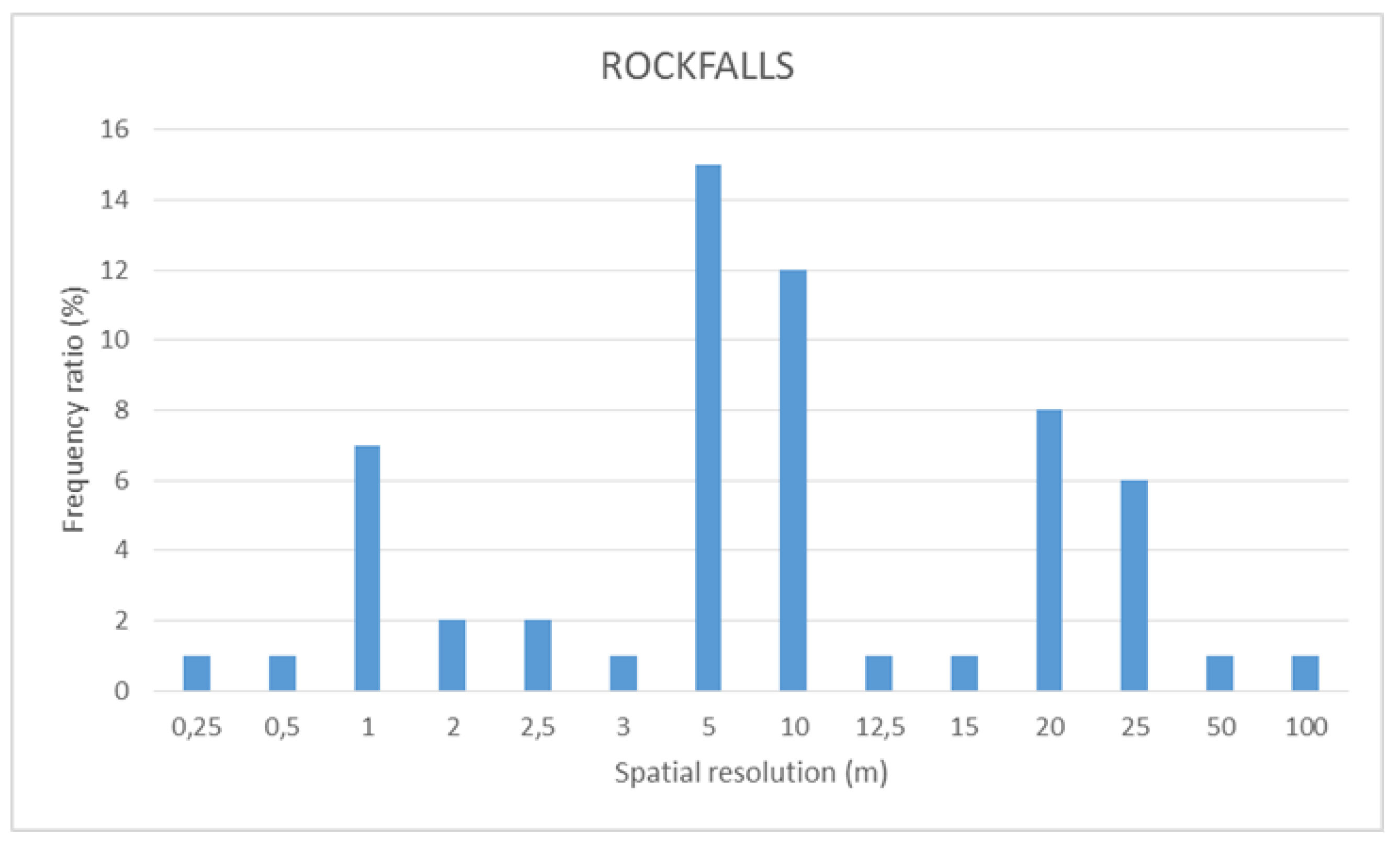
5.2. The Effect of DEM Resolution on Rockfalls
6. Conclusions
7. Future Work
Author Contributions
Funding
Institutional Review Board Statement
Informed Consent Statement
Data Availability Statement
Acknowledgments
Conflicts of Interest
Abbreviations
| Acronyms | Meaning |
| MODELS | |
| DEM | Digital Elevation Model |
| DTM | Digital Terrain Model |
| DSM | Digital Surface Model |
| INDEXES | |
| TPI | Topographic Position Index |
| TWI | Topographic Wetness Index |
| TRI | Topographic Roughness Index |
| CTI | Compound Topographic Index |
| STI | Sediment Transport Index |
| SPI | Stream Power Index |
| NDVI | Normalized Difference Vegetation Index |
| SL | Slope |
| METHODS | |
| AHP | Analytical Hierarchy Process |
| PLR | Probabilistic Likelihood Ratio |
| FM | Fuzzy Method |
| HL | Hybrid Likelihood |
| TIN | Triangular Irregular Networks |
| ANN | Artificial Neural Networks |
| FBPNN | Feedforward Back-Propagation Neural Network |
| AUC | Area under the Curve |
| ROC | Receiver Operating Characteristic |
| GPS | Ground Position System |
| API | Aerial Photo Interpretation |
| TPI | Terrestrial Photo Interpretation |
| InSAR | Satellite Radar Interferometry |
| SI | Satellite Imagery |
| ALS | Aerial Laser Scanning |
| TLS | Terrestrial Laser Scanning |
| LiDAR | Light Detection and Ranging |
| KM | Kriging Method |
| LM | Lumped Mass Method |
| WofE | Weights of Evidence |
| FR | Frequency Ratio |
| CF | Certainty Factor |
| DA | Discriminant Analysis |
| LR | Logical Regression |
| MM | Matrix Method |
| RFEM | Random Finite Element Method |
| SLBL | Sloping Local Base Level |
| MCM | Monte Carlo Method |
| DEM/DTM | |
| ALOS | Advanced Land Observing Satellite |
| SRTM | Shuttle Radar Topography Mission |
| ASTER | Advanced Spaceborne Thermal Emission and Reflection Radiometer |
| TanDEM-X | TerraSAR-X add-on for Digital Elevation Measurement |
| MOLA | Mars Orbiter Laser Altimeter |
| HRSC | High-Resolution Stereo Camera on Mars Express |
References
- Florinsky, I.V. Accuracy of local topographic variables derived from digital elevation models. Int. J. Geogr. Inf. Sci. 1998, 12, 47–62. [Google Scholar] [CrossRef]
- Maune, D.F.; Maitra, J.B.; McKay, E.J. Accuracy Standards. In Digital Elevation Models and Applications: The DEM Users Manual; American Society for Photogrammetry and Remote Sensing: Bethesda, MD, USA, 2001; pp. 61–82. [Google Scholar]
- Sauchyn, D.J.; Gardner, J.S. Morphometry of open rock basins, Kananaskis area, Canadian Rocky Mountains. Can. J. Earth Sci. 1983, 20, 409–419. [Google Scholar] [CrossRef]
- Toppe, R. Terrain models: A tool for natural hazard mapping. IAHS Publication 1987, 162, 629–638. [Google Scholar]
- Gao, J. Identification of topographic settings conducive to landsliding from dem in Nelson county, Virginia, USA. Earth Surf. Process. Landf. 1993, 18, 579–591. [Google Scholar] [CrossRef]
- Borga, M.; Dalla Fontana, G.; Da Ros, D.; Marchi, L. Shallow landslide hazard assessment using a physically based model and digital elevation data. Environ. Geol. 1998, 35, 81–88. [Google Scholar] [CrossRef]
- Pack, R.T.; Tarboton, D.G.; Goodwin, C.N. The SINMAP Approach to Terrain Stability Mapping. In Proceedings of the 8th Congress of the International Association of Engineering Geology, Vancouver, BC, Canada, 21–25 September 1998. [Google Scholar]
- Dietrich, W.E.; Bellugi, D.G.; Sklar, L.S.; Stock, J.D.; Heimsath, A.M.; Roering, J.J. Geomorphic Transport Laws for Predicting Landscape form and Dynamics. Geophys. Monogr. Ser. 2013, 103–132. [Google Scholar] [CrossRef]
- Jaboyedoff, M.; Baillifard, F.; Couture, R.; Locat, J.; Locat, P. Toward preliminary hazard assessment using DEM topographic analysis and simple mechanical modeling by means of sloping local base level. Part B. In Landslides Evaluation and Stabilization; Balkema: Boca Raton, FL, USA, 2004; pp. 199–205. [Google Scholar]
- Miner, A.; Flentje, P.; Mazengarb, C.; Windle, D.J. Landslide Recognition Using LiDAR Derived Digital Elevation Models-Lessons Learnt from Selected Australian Examples. In Proceedings of the 11th IAEG Congress of the International Association of Engineering Geology and the Environment, Auckland, New Zealand, 5–10 September 2010; pp. 1–9. [Google Scholar]
- Fenton, G.A.; McLean, A.; Nadim, F.; Griffiths, D.V. Landslide hazard assessment using digital elevation models. Can. Geotech. J. 2013, 50, 620–631. [Google Scholar] [CrossRef]
- Ciampalini, A.; Raspini, F.; Frodella, W.; Bardi, F.; Bianchini, S.; Moretti, S. The effectiveness of high-resolution LiDAR data combined with PSInSAR data in landslide study. Landslides 2015, 13, 399–410. [Google Scholar] [CrossRef]
- Pradhan, B.; Sameen, M.I. Effects of the Spatial Resolution of Digital Elevation Models and Their Products on Landslide Susceptibility Mapping. Laser Scanning Appl. Landslide Assess. 2017, 133–150. [Google Scholar] [CrossRef]
- Depountis, N.; Nikolakopoulos, K.; Kavoura, K.; Sabatakakis, N. Description of a GIS-based rockfall hazard assessment methodology and its application in mountainous sites. Bull. Eng. Geol. Environ. 2019. [Google Scholar] [CrossRef]
- Loye, A.; Jaboyedoff, M.; Pedrazzini, A. Identification of potential rockfall source areas at a regional scale using a DEM-based geomorphometric analysis. Nat. Hazards Earth Syst. Sci. 2009, 9, 1643–1653. [Google Scholar] [CrossRef]
- Jaboyedoff, M.; Baillifard, F.; Couture, R.; Locat, J.; Locat, P. Toward preliminary hazard assessment using DEM topographic analysis and simple mechanical modeling by means of sloping local base level. Part A. In Landslides Evaluation and Stabilization; Balkema: Boca Raton, FL, USA, 2004; pp. 191–198. [Google Scholar]
- Saleem, N.; Huq, M.; Twumasi, N.Y.D.; Javed, A.; Sajjad, A. Parameters derived from and/or used with digital elevation models (DEMs) for landslide susceptibility mapping and landslide risk assessment: A review. ISPRS Int. J. Geo Inf. 2019, 8, 545. [Google Scholar] [CrossRef]
- Chang, K.T.; Doub, J.; Changc, Y.; Kuo, C.P.; Xu, K.M.; Liu, J.K. Spatial resolution effects of digital terrain models on landslide susceptibility analysis. Int. Arch. Photogramm. Remote Sens. Spat. Inf. Sci. 2016, 8. [Google Scholar] [CrossRef]
- Kawabata, D.; Bandibas, J. Landslide susceptibility mapping using geological data, a DEM from ASTER images and an Artificial Neural Network (ANN). Geomorphology 2009, 113, 97–109. [Google Scholar] [CrossRef]
- Pawluszek, K.; Borkowski, A. Impact of DEM-derived factors and analytical hierarchy process on landslide susceptibility mapping in the region of Rożnów Lake, Poland. Nat. Hazards 2017, 86, 919–952. [Google Scholar] [CrossRef]
- Mahalingam, R.; Olsen, M.J.; O’Banion, M.S. Evaluation of landslide susceptibility mapping techniques using lidar-derived conditioning factors (Oregon case study). Geomat. Nat. Hazards Risk 2016, 7, 1884–1907. [Google Scholar] [CrossRef]
- Chen, Q.; Liu, X.; Liu, C.; Ji, R. Impact Analysis of Different Spatial Resolution DEM on Object-Oriented Landslide Extraction from High Resolution Remote Sensing Images. In Proceedings of the 2013 Ninth International Conference on Natural Computation (ICNC), Shenyang, China, 23–25 July 2013; IEEE. pp. 940–945. [Google Scholar] [CrossRef]
- Kasai, M.; Ikeda, M.; Asahina, T.; Fujisawa, K. LiDAR-derived DEM evaluation of deep-seated landslides in a steep and rocky region of Japan. Geomorphology 2009, 113, 57–69. [Google Scholar] [CrossRef]
- Ku, C.Y. Assessing Rockfall Hazards Using a Three-Dimensional Numerical Model Based on High Resolution DEM. In Proceedings of the Twenty-second International Offshore and Polar Engineering Conference, Rhodes, Greece, 17–22 June 2012; International Society of Offshore and Polar Engineers: Cupertino, CA, USA. [Google Scholar]
- Calvello, M.; Cascini, L.; Mastroianni, S. Landslide zoning over large areas from a sample inventory by means of scale-dependent terrain units. Geomorphology 2013, 182, 33–48. [Google Scholar] [CrossRef]
- Corominas, J.; van Westen, C.; Frattini, P.; Cascini, L.; Malet, J.-P.; Fotopoulou, S.; Catani, F.; Van Den Eeckhaut, M.; Mavrouli, O.; Smith, J.T. Recommendations for the quantitative analysis of landslide risk. Bull. Eng. Geol. Environ. 2013. [Google Scholar] [CrossRef]
- Mandal, S.; Maiti, R. Semi-Quantitative Approaches for Landslide Assessment and Prediction; Springer: Singapore, 2015; pp. 57–93. [Google Scholar] [CrossRef]
- Martha, T.R.; Kerle, N.; Jetten, V.; van Westen, C.J.; Kumar, K.V. Characterising spectral, spatial and morphometric properties of landslides for semi-automatic detection using object-oriented methods. Geomorphology 2010, 116, 24–36. [Google Scholar] [CrossRef]
- Costanzo, D.; Rotigliano, E.; Irigaray, C.; Jiménez-Perálvarez, J.D.; Chacón, J. Factors selection in landslide susceptibility modelling on large scale following the gis matrix method: Application to the river Beiro basin (Spain). Nat. Hazards Earth Syst. Sci. 2012, 12, 327–340. [Google Scholar] [CrossRef]
- Oh, H.J.; Kadavi, P.R.; Lee, C.W.; Lee, S. Evaluation of landslide susceptibility mapping by evidential belief function, logistic regression and support vector machine models. Geomat. Nat. Hazards Risk 2018, 9, 1053–1070. [Google Scholar] [CrossRef]
- Ercanoglu, M.; Gokceoglu, C. Use of fuzzy relations to produce landslide susceptibility map of a landslide prone area (West Black Sea Region, Turkey). Eng. Geol. 2004, 75, 229–250. [Google Scholar] [CrossRef]
- Gorsevski, P.V.; Jankowski, P. Discerning landslide susceptibility using rough sets. Comput. Environ. Urban Syst. 2008, 32, 53–65. [Google Scholar] [CrossRef]
- Yesilnacar, E.; Topal, T. Landslide susceptibility mapping: A comparison of logistic regression and neural networks methods in a medium scale study, Hendek region (Turkey). Eng. Geol. 2005, 79, 251–266. [Google Scholar] [CrossRef]
- Dagdelenler, G.; Nefeslioglu, H.A.; Gokceoglu, C. Modification of seed cell sampling strategy for landslide susceptibility mapping: An application from the Eastern part of the Gallipoli Peninsula (Canakkale, Turkey). Bull. Eng. Geol. Environ. 2015, 75, 575–590. [Google Scholar] [CrossRef]
- Liu, J.; Duan, Z. Quantitative Assessment of Landslide Susceptibility Comparing Statistical Index, Index of Entropy, and Weights of Evidence in the Shangnan Area, China. Entropy 2018, 20, 868. [Google Scholar] [CrossRef]
- Chen, W.; Panahi, M.; Tsangaratos, P.; Shahabi, H.; Ilia, I.; Panahi, S.; Li, S.; Jaafari, A.; Ahmad, B.B. Applying population-based evolutionary algorithms and a neuro-fuzzy system for modeling landslide susceptibility. CATENA 2019, 172, 212–231. [Google Scholar] [CrossRef]
- Pourghasemi, H.R.; Mohammady, M.; Pradhan, B. Landslide susceptibility mapping using index of entropy and conditional probability models in GIS: Safarood Basin, Iran. CATENA 2012, 97, 71–84. [Google Scholar] [CrossRef]
- Martha, T.R.; van Westen, C.J.; Kerle, N.; Jetten, V.; Vinod Kumar, K. Landslide hazard and risk assessment using semi-automatically created landslide inventories. Geomorphology 2013, 184, 139–150. [Google Scholar] [CrossRef]
- Zhu, A.-X.; Miao, Y.; Yang, L.; Bai, S.; Liu, J.; Hong, H. Comparison of the presence-only method and presence-absence method in landslide susceptibility mapping. CATENA 2018, 171, 222–233. [Google Scholar] [CrossRef]
- Dou, J.; Yunus, A.P.; Tien Bui, D.; Merghadi, A.; Sahana, M.; Zhu, Z.; Chen, C.-W.; Khosravi, K.; Yang, Y.; Pham, B.T. Assessment of advanced random forest and decision tree algorithms for modeling rainfall-induced landslide susceptibility in the Izu-Oshima Volcanic Island, Japan. Sci. Total Environ. 2019. [Google Scholar] [CrossRef]
- Ozdemir, A.; Altural, T. A comparative study of frequency ratio, weights of evidence and logistic regression methods for landslide susceptibility mapping: Sultan Mountains, SW Turkey. J. Asian Earth Sci. 2013, 64, 180–197. [Google Scholar] [CrossRef]
- Jaboyedoff, M.; Couture, R.; Locat, P. Structural analysis of Turtle Mountain (Alberta) using digital elevation model: Toward a progressive failure. Geomorphology 2009, 103, 5–16. [Google Scholar] [CrossRef]
- Van Dijke, J.J.; van Westen, C.J. Rockfall hazard: A geomorphologic application of neighbourhood analysis with ILWIS. ITC J. 1990, 1, 40–44. [Google Scholar]
- Baillifard, F.; Jaboyedoff, M.; Sartori, M. Rockfall hazard mapping along a mountainous road in Switzerland using a GIS-based parameter rating approach. Nat. Hazards Earth Syst. Sci. 2003, 3, 435–442. [Google Scholar] [CrossRef]
- Crosta, G.B.; Agliardi, F. Parametric evaluation of 3D dispersion of rockfall trajectories. Nat. Hazards Earth Syst. Sci. 2004, 4, 583–598. [Google Scholar] [CrossRef]
- Fuchs, M.; Torizin, J.; Kühn, F. The effect of DEM resolution on the computation of the factor of safety using an infinite slope model. Geomorphology 2014, 224, 16–26. [Google Scholar] [CrossRef]
- Devkota, K.C.; Regmi, A.D.; Pourghasemi, H.R.; Yoshida, K.; Pradhan, B.; Ryu, I.C.; Dhital, M.R.; Althuwaynee, O.F. Landslide susceptibility mapping using certainty factor, index of entropy and logistic regression models in GIS and their comparison at Mugling–Narayanghat road section in Nepal Himalaya. Nat. Hazards 2012, 65, 135–165. [Google Scholar] [CrossRef]
- Ciampalini, A.; Raspini, F.; Bianchini, S.; Frodella, W.; Bardi, F.; Lagomarsino, D.; Di Traglia, F.; Moretti, S.; Proietti, C.; Pagliara, P. Remote sensing as tool for development of landslide databases: The case of the Messina Province (Italy) geodatabase. Geomorphology 2015, 249, 103–118. [Google Scholar] [CrossRef]
- Vanacker, V.; Vanderschaeghe, M.; Govers, G.; Willems, E.; Poesen, J.; Deckers, J.; De Bievre, B. Linking hydrological, infinite slope stability and land-use change models through GIS for assessing the impact of deforestation on slope stability in high Andean watersheds. Geomorphology 2003, 52, 299–315. [Google Scholar] [CrossRef]
- Yilmaz, I. Landslide susceptibility mapping using frequency ratio, logistic regression, artificial neural networks and their comparison: A case study from Kat landslides (Tokat—Turkey). Comput. Geosci. 2009, 35, 1125–1138. [Google Scholar] [CrossRef]
- Chacón, J.; Irigaray, C.; Fernández, T.; El Hamdouni, R. Engineering geology maps: Landslides and geographical information systems. Bull. Eng. Geol. Environ. 2006, 65, 341–411. [Google Scholar] [CrossRef]
- Oh, H.-J.; Park, N.-W.; Lee, S.-S.; Lee, S. Extraction of landslide-related factors from ASTER imagery and its application to landslide susceptibility mapping. Int. J. Remote Sens. 2012, 33, 3211–3231. [Google Scholar] [CrossRef]
- Reichenbach, P.; Rossi, M.; Malamud, B.D.; Mihir, M.; Guzzetti, F. A review of statistically-based landslide susceptibility models. Earth Sci. Rev. 2018, 180, 60–91. [Google Scholar] [CrossRef]
- Kaur, H.; Gupta, S.; Parkash, S.; Thapa, R. Application of geospatial technologies for multi-hazard mapping and characterization of associated risk at local scale. Ann. GIS 2018, 24, 33–46. [Google Scholar] [CrossRef]
- Cascini, L.C.J.R.J.O.; Bonnard, C.; Corominas, J.; Jibson, R.; Montero-Olarte, J. Landslide hazard and risk zoning for urban planning and development. In Landslide Risk Management; Taylor and Francis: London, UK, 2005; pp. 199–235. [Google Scholar]
- Pradhan, B.; Sezer, E.A.; Gokceoglu, C.; Buchroithner, M.F. Landslide Susceptibility Mapping by Neuro-Fuzzy Approach in a Landslide-Prone Area (Cameron Highlands, Malaysia). IEEE Trans. Geosci. Remote Sens. 2010, 48, 4164–4177. [Google Scholar] [CrossRef]
- Lee, S.; Talib, J.A. Probabilistic landslide susceptibility and factor effect analysis. Environ. Geol. 2005, 47, 982–990. [Google Scholar] [CrossRef]
- Pradhan, B.; Lee, S. Landslide susceptibility assessment and factor effect analysis: Backpropagation artificial neural networks and their comparison with frequency ratio and bivariate logistic regression modelling. Environ. Model. Softw. 2010, 25, 747–759. [Google Scholar] [CrossRef]
- Niethammer, U.; James, M.R.; Rothmund, S.; Travelletti, J.; Joswig, M. UAV-based remote sensing of the Super-Sauze landslide: Evaluation and results. Eng. Geol. 2012, 128, 2–11. [Google Scholar] [CrossRef]
- Mahalingam, R.; Olsen, M.J. Evaluation of the influence of source and spatial resolution of DEMs on derivative products used in landslide mapping. Geomat. Nat. Hazards Risk 2015, 7, 1835–1855. [Google Scholar] [CrossRef]
- Akgun, A.; Dag, S.; Bulut, F. Landslide susceptibility mapping for a landslide-prone area (Findikli, NE of Turkey) by likelihood-frequency ratio and weighted linear combination models. Environ. Geol. 2007, 54, 1127–1143. [Google Scholar] [CrossRef]
- Bagherzadeh, A.; Mansouri Daneshvar, M.R. Mapping of landslide hazard zonation using GIS at Golestan watershed, northeast of Iran. Arab. J. Geosci. 2012, 6, 3377–3388. [Google Scholar] [CrossRef]
- Lee, S.; Ryu, J.-H.; Lee, M.-J.; Won, J.-S. The Application of Artificial Neural Networks to Landslide Susceptibility Mapping at Janghung, Korea. Math. Geol. 2006, 38, 199–220. [Google Scholar] [CrossRef]
- Frattini, P.; Crosta, G.B.; Agliardi, F.; Imposimato, S. Challenging Calibration in 3D Rockfall Modelling. Landslide Sci. Pract. 2013, 169–175. [Google Scholar] [CrossRef]
- Stock, G.M.; Bawden, G.W.; Green, J.K.; Hanson, E.; Downing, G.; Collins, B.D.; Bond, S.; Leslar, M. High-resolution three-dimensional imaging and analysis of rock falls in Yosemite Valley, California. Geosphere 2011, 7, 573–581. [Google Scholar] [CrossRef]
- Guzzetti, F.; Reichenbach, P.; Ghigi, S. Rockfall Hazard and Risk Assessment: Along a Transportation Corridor in the Nera Valley, Central Italy. Environ. Manag. 2004, 34, 191–208. [Google Scholar] [CrossRef]
- Van Westen, C.J.; van Asch, T.W.J.; Soeters, R. Landslide hazard and risk zonation—why is it still so difficult? Bull. Eng. Geol. Environ. 2005, 65, 167–184. [Google Scholar] [CrossRef]
- Rasyid, A.R.; Bhandary, N.P.; Yatabe, R. Performance of frequency ratio and logistic regression model in creating GIS based landslides susceptibility map at Lompobattang Mountain, Indonesia. Geoenviron. Dis. 2016, 3. [Google Scholar] [CrossRef]
- Wang, Q.; Li, W.; Wu, Y.; Pei, Y.; Xie, P. Application of statistical index and index of entropy methods to landslide susceptibility assessment in Gongliu (Xinjiang, China). Environ. Earth Sci. 2016, 75. [Google Scholar] [CrossRef]
- Juliev, M.; Mergili, M.; Mondal, I.; Nurtaev, B.; Pulatov, A.; Hübl, J. Comparative analysis of statistical methods for landslide susceptibility mapping in the Bostanlik District, Uzbekistan. Sci. Total Environ. 2018. [Google Scholar] [CrossRef]
- Pesci, A.; Baldi, P.; Bedin, A.; Casula, G.; Cenni, N.; Fabris, M.; Loddo, F.; Moram, M.; Bacchetti, M. Digital elevation models for landslide evolution monitoring: Application on two areas located in the Reno River Valley (Italy). Ann. Geophys. 2004, 74, 4. Available online: http://hdl.handle.net/2122/836 (accessed on 8 April 2021).
- Ardizzone, F.; Cardinali, M.; Galli, M.; Guzzetti, F.; Reichenbach, P. Identification and mapping of recent rainfall-induced landslides using elevation data collected by airborne Lidar. Nat. Hazards Earth Syst. Sci. 2007, 7, 637–650. [Google Scholar] [CrossRef]
- Jaboyedoff, M.; Oppikofer, T.; Abellán, A.; Derron, M.-H.; Loye, A.; Metzger, R.; Pedrazzini, A. Use of LIDAR in landslide investigations: A review. Nat. Hazards 2010, 61, 5–28. [Google Scholar] [CrossRef]
- Colesanti, C.; Wasowski, J. Investigating landslides with space-borne Synthetic Aperture Radar (SAR) interferometry. Eng. Geol. 2006, 88, 173–199. [Google Scholar] [CrossRef]
- Zieher, T.; Formanek, T.; Bremer, M.; Meissl, G.; Rutzinger, M. Digital Terrain Model Resolution and its Influence on Estimating the Extent of Rockfall Areas. Trans. GIS 2012, 16, 691–699. [Google Scholar] [CrossRef]
- Günther, A.; Carstensen, A.; Pohl, W. Automated sliding susceptibility mapping of rock slopes. Nat. Hazards Earth Syst. Sci. 2004, 4, 95–102. [Google Scholar] [CrossRef]
- Read, R.S.; Langenberg, W.; Cruden, D.; Field, M.; Stewart, R.; Bland, H.; Chen, Z.; Froese, C.R.; Cavers, D.S.; Bidwell, A.K. Frank Slide a century later: The Turtle Mountain monitoring project. In Landslide Risk Management; CRC Press: Boca Raton, FL, USA, 2005; pp. 713–723. [Google Scholar]
- Glenn, N.F.; Streutker, D.R.; Chadwick, D.J.; Thackray, G.D.; Dorsch, S.J. Analysis of LiDAR-derived topographic information for characterizing and differentiating landslide morphology and activity. Geomorphology 2006, 73, 131–148. [Google Scholar] [CrossRef]
- Gorum, T.; Fan, X.; van Westen, C.J.; Huang, R.Q.; Xu, Q.; Tang, C.; Wang, G. Distribution pattern of earthquake-induced landslides triggered by the 12 May 2008 Wenchuan earthquake. Geomorphology 2011, 133, 152–167. [Google Scholar] [CrossRef]
- Kakavas, M.; Kyriou, A.; Nikolakopoulos, K.G. Assessment of Freely Available DSMs for Landslide-Rockfall Studies. In Proceedings of the Earth Resources and Environmental Remote Sensing/GIS Applications XI, Edinburgh, UK, 20 September 2020; International Society for Optics and Photonics. Volume 11534, p. 115340R. [Google Scholar] [CrossRef]
- Keijsers, J.G.S.; Schoorl, J.M.; Chang, K.-T.; Chiang, S.-H.; Claessens, L.; Veldkamp, A. Calibration and resolution effects on model performance for predicting shallow landslide locations in Taiwan. Geomorphology 2011, 133, 168–177. [Google Scholar] [CrossRef]
- Frattini, P.; Crosta, G.; Carrara, A.; Agliardi, F. Assessment of rockfall susceptibility by integrating statistical and physically-based approaches. Geomorphology 2008, 94, 419–437. [Google Scholar] [CrossRef]
- Booth, A.M.; Roering, J.J.; Perron, J.T. Automated landslide mapping using spectral analysis and high-resolution topographic data: Puget Sound lowlands, Washington, and Portland Hills, Oregon. Geomorphology 2009, 109, 132–147. [Google Scholar] [CrossRef]
- Ravanel, L.; Allignol, F.; Deline, P.; Gruber, S.; Ravello, M. Rock falls in the Mont Blanc Massif in 2007 and 2008. Landslides 2010, 7, 493–501. [Google Scholar] [CrossRef]
- Mancini, F.; Ceppi, C.; Ritrovato, G. GIS and statistical analysis for landslide susceptibility mapping in the Daunia area, Italy. Nat. Hazards Earth Syst. Sci. 2010, 10, 1851–1864. [Google Scholar] [CrossRef]
- Fernández, T.; Irigaray, C.; El Hamdouni, R.; Chacón, J. Methodology for Landslide Susceptibility Mapping by Means of a GIS. Application to the Contraviesa Area (Granada, Spain). Nat. Hazards 2003, 30, 297–308. [Google Scholar] [CrossRef]
- Bianchini, S.; Solari, L.; Casagli, N. A GIS-Based Procedure for Landslide Intensity Evaluation and Specific Risk Analysis Supported by Persistent Scatterers Interferometry (PSI). Remote Sens. 2017, 9, 1093. [Google Scholar] [CrossRef]
- Guzzetti, F.; Carrara, A.; Cardinali, M.; Reichenbach, P. Landslide hazard evaluation: A review of current techniques and their application in a multi-scale study, Central Italy. Geomorphology 1999, 31, 181–216. [Google Scholar] [CrossRef]
- Acosta, E.; Agliardi, F.; Crosta, G.B.; Rıos Aragues, S. Regional Rockfall Hazard Assessment in the Benasque Valley (Central Pyrenees) Using a 3D Numerical Approach. In Proceedings of the 4th EGS Plinius Conference—Mediterranean Storms, Mallorca, Spain, 2–4 October 2002; pp. 555–563. [Google Scholar]
- Sartori, M.; Baillifard, F.; Jaboyedoff, M.; Rouiller, J.-D. Kinematics of the 1991 Randa rockslides (Valais, Switzerland). Nat. Hazards Earth Syst. Sci. 2003, 3, 423–433. [Google Scholar] [CrossRef]
- Agliardi, F.; Crosta, G.; Zanchi, A. Structural constraints on deep-seated slope deformation kinematics. Eng. Geol. 2001, 59, 83–102. [Google Scholar] [CrossRef]
- Thiery, Y.; Sterlacchini, S.; Malet, J.P.; Puissant, A.; Remaître, A.; Maquaire, O. Strategy to Reduce Subjectivity in Landslide Susceptibility Zonation by GIS in Complex Mountainous Environments. In Proceedings of the 7th AGILE Conference on GIScience, Heraklion, Greece, 29 April–1 May 2004; pp. 623–634. [Google Scholar]
- Yu, M.; Huang, Y.; Xu, Q.; Guo, P.; Dai, Z. Application of virtual earth in 3D terrain modeling to visual analysis of large-scale geological disasters in mountainous areas. Environ. Earth Sci. 2016, 75. [Google Scholar] [CrossRef]
- Carrara, A.; Guzzetti, F.; Cardinali, M.; Reichenbach, P. Use of GIS technology in the prediction and monitoring of landslide hazard. Nat. Hazards 1999, 20, 117–135. [Google Scholar] [CrossRef]
- Nichol, J.; Wong, M.S. Satellite remote sensing for detailed landslide inventories using change detection and image fusion. Int. J. Remote Sens. 2005, 26, 1913–1926. [Google Scholar] [CrossRef]
- Huang, Y.; Yu, M.; Xu, Q.; Sawada, K.; Moriguchi, S.; Yashima, A.; Liu, C.; Xue, L. InSAR-derived digital elevation models for terrain change analysis of earthquake-triggered flow-like landslides based on ALOS/PALSAR imagery. Environ. Earth Sci. 2014, 73, 7661–7668. [Google Scholar] [CrossRef]
- Chigira, M.; Wu, X.; Inokuchi, T.; Wang, G. Landslides induced by the 2008 Wenchuan earthquake, Sichuan, China. Geomorphology 2010, 118, 225–238. [Google Scholar] [CrossRef]
- Abellán, A.; Vilaplana, J.M.; Martínez, J. Application of a long-range Terrestrial Laser Scanner to a detailed rockfall study at Vall de Núria (Eastern Pyrenees, Spain). Eng. Geol. 2006, 88, 136–148. [Google Scholar] [CrossRef]
- Palma, B.; Parise, M.; Reichenbach, P.; Guzzetti, F. Rockfall hazard assessment along a road in the Sorrento Peninsula, Campania, southern Italy. Nat. Hazards 2011, 61, 187–201. [Google Scholar] [CrossRef]
- Tarolli, P.; Dalla Fontana, G. Hillslope-to-valley transition morphology: New opportunities from high resolution DTMs. Geomorphology 2009, 113, 47–56. [Google Scholar] [CrossRef]
- Žabota, B.; Repe, B.; Kobal, M. Influence of digital elevation model resolution on rockfall modelling. Geomorphology 2018. [Google Scholar] [CrossRef]
- Jaboyedoff, M.; Choffet, M.; Derron, M.-H.; Horton, P.; Loye, A.; Longchamp, C.; Mazotti, B.; Michoud, C.; Pedrazzini, A. Preliminary Slope Mass Movement Susceptibility Mapping Using DEM and LiDAR DEM. In Terrigenous Mass Movements; Springer: Cham, Switzerland, 2012; pp. 109–170. [Google Scholar] [CrossRef]
- Lan, H.; Derek Martin, C.; Lim, C.H. RockFall analyst: A GIS extension for three-dimensional and spatially distributed rockfall hazard modeling. Comput. Geosci. 2007, 33, 262–279. [Google Scholar] [CrossRef]
- Nikolakopoulos, K.; Depountis, N.; Vagenas, N.; Kavoura, K.; Vlaxaki, E.; Kelasidis, G.; Sabatakakis, N. Rockfall Risk Evaluation Using Geotechnical Survey, Remote Sensing Data, and GIS: A Case Study from Western Greece. In Proceedings of the Third International Conference on Remote Sensing and Geoinformation of the Environment (RSCy2015), Paphos, Cyprus, 19 June 2015. [Google Scholar] [CrossRef]
- Agliardi, F.; Crosta, G.B. High resolution three-dimensional numerical modelling of rockfalls. Int. J. Rock Mech. Min. Sci. 2003, 40, 455–471. [Google Scholar] [CrossRef]
- Guzzetti, F.; Reichenbach, P.; Wieczorek, G.F. Rockfall hazard and risk assessment in the Yosemite Valley, California, USA. Nat. Hazards Earth Syst. Sci. 2003, 3, 491–503. [Google Scholar] [CrossRef]
- Crosta, G.B.; Agliardi, F. A methodology for physically based rockfall hazard assessment. Nat. Hazards Earth Syst. Sci. 2003, 3, 407–422. [Google Scholar] [CrossRef]
- Lee, S.; Choi, J.; Woo, I. The effect of spatial resolution on the accuracy of landslide susceptibility mapping: A case study in Boun, Korea. Geosci. J. 2004, 8, 51–60. [Google Scholar] [CrossRef]
- Aksoy, H.; Ercanoglu, M. Determination of the rockfall source in an urban settlement area by using a rule-based fuzzy evaluation. Nat. Hazards Earth Syst. Sci. 2006, 6, 941–954. [Google Scholar] [CrossRef][Green Version]
- Derron, M.-H.; Jaboyedoff, M.; Blikra, L.H. Preliminary assessment of rockslide and rockfall hazards using a DEM (Oppstadhornet, Norway). Nat. Hazards Earth Syst. Sci. 2005, 5, 285–292. [Google Scholar] [CrossRef]
- Qin, C.-Z.; Bao, L.-L.; Zhu, A.-X.; Wang, R.-X.; Hu, X.-M. Uncertainty due to DEM error in landslide susceptibility mapping. Int. J. Geogr. Inf. Sci. 2013, 27, 1364–1380. [Google Scholar] [CrossRef]
- Volkwein, A.; Schellenberg, K.; Labiouse, V.; Agliardi, F.; Berger, F.; Bourrier, F.; Dorren, L.K.A.; Gerber, W.; Jaboyedoff, M. Rockfall characterisation and structural protection—A review. Nat. Hazards Earth Syst. Sci. 2011, 11, 2617–2651. [Google Scholar] [CrossRef]
- Stevens, W.D. RocFall, a Tool for Probabilistic Analysis, Design of Remedial Measures and Prediction of Rockfalls. Master’s Thesis, University of Toronto, Toronto, ON, Canada, 1998. [Google Scholar]
- Corona, C.; Trappmann, D.; Stoffel, M. Parameterization of rockfall source areas and magnitudes with ecological recorders: When disturbances in trees serve the calibration and validation of simulation runs. Geomorphology 2013, 202, 33–42. [Google Scholar] [CrossRef]
- Dorren, L.K.A. Rockyfor3D (v5.0) Revealed—Transparent Description of the Complete 3D Rockfall Model; EcorisQ Paper: Geneva, Switzerland, 2012. [Google Scholar]
- Geostru GeoRock. User Guide; Geostru Software: Cosenza, Italy, 2004. [Google Scholar]
- Geostru GeoRock. 3D User Guide; Geostru Software: Cosenza, Italy, 2009. [Google Scholar]
- Bühler, Y.; Christen, M.; Glover, J.; Bartelt, P. Significance of Digital Elevation Model Resolution for Numerical Rockfall Simulations. In Proceedings of the 3rd International Symposium Rock Slope Stability C2ROP, Lyon, France, 15–17 November 2016; pp. 15–17. [Google Scholar]
- Pack, R.T.; Tarboton, D.G.; Goodwin, C.N. Terrain Stability Mapping with SINMAP, Technical Description and Users Guide for Version 1.00. 1998. Available online: https://www.semanticscholar.org/paper/Terrain-Stability-Mapping-with-SINMAP%2C-technical-Pack-Tarboton/b55931b905be0d789e6c719e7ba0e56bfbea7d48 (accessed on 8 April 2021).
- CREALP. Software for the Analysis of Spatial Distribution of Discontinuities in Cliffs: Mattercliff; CREALP: Sion, Switzerland, 2003; Available online: http://www.crealp.ch/ (accessed on 8 April 2021).
- Jaboyedoff, M.; Baillifard, F.; Philippossian, F.; Rouiller, J.-D. Assessing fracture occurrence using “weighted fracturing density”: A step towards estimating rock instability hazard. Nat. Hazards Earth Syst. Sci. 2004, 4, 83–93. [Google Scholar] [CrossRef]
- Guzzetti, F.; Crosta, G.; Detti, R.; Agliardi, F. STONE: A computer program for the three-dimensional simulation of rock-falls. Comput. Geosci. 2002, 28, 1079–1093. [Google Scholar] [CrossRef]
- Scioldo, G. User Guide ISOMAP & ROTOMAP—3D Surface Modelling and Rockfall Analysis; Geo&Soft International: Torino, Italy, 2006. [Google Scholar]
- Jaboyedoff, M.; Metzger, R.; Oppikofer, T.; Couture, R.; Derron, M.H.; Locat, J.; Turmel, D. New Insight Techniques to Analyze Rock-Slope Relief Using DEM and 3Dimaging Cloud Points: COLTOP-3D Software. In Proceedings of the 1st Canada-US Rock Mechanics Symposium, Vancouver, BC, Canada, 27–31 May 2007. American Rock Mechanics Association. [Google Scholar]
- Jaboyedoff, M.; Labiouse, V. Preliminary Assessment of Rockfall Hazard Based on GIS Data. In Proceedings of the 10th ISRM Congress, Sandton, South Africa, 8–12 September 2003; International Society for Rock Mechanics and Rock Engineering: Lisbon, Portugal. [Google Scholar]
- Jaboyedoff, M.; Labiouse, V. Technical Note: Preliminary estimation of rockfall runout zones. Nat. Hazards Earth Syst. Sci. 2011, 11, 819–828. [Google Scholar] [CrossRef]
- International Institute for Aerospace Survey and Earth Sciences. ILWIS 2.2 for Windows, the Integral Land and Water Information System: Reference Guide; ILWIS Development ITC: Enschede, The Netherlands, 1999. [Google Scholar]
- Carrara, A.; Cardinali, M.; Detti, R.; Guzzetti, F.; Pasqui, V.; Reichenbach, P. GIS techniques and statistical models in evaluating landslide hazard. Int. J. Rock Mech. Min. Sci. Geomech. Abstr. 1991, 29, A102. [Google Scholar] [CrossRef]
- Claessens, L.; Heuvelink, G.B.M.; Schoorl, J.M.; Veldkamp, A. DEM resolution effects on shallow landslide hazard and soil redistribution modelling. Earth Surf. Proc. Landf. 2005, 30, 461–477. [Google Scholar] [CrossRef]
- McLean, A. Landslide risk assessment using digital elevation models. Can. Geotech. J. 2011. [Google Scholar] [CrossRef]
- Marquínez, J.; Menéndez Duarte, R.; Farias, P.; Jiménez Sánchez, M. Predictive GIS-Based Model of Rockfall Activity in Mountain Cliffs. Nat. Hazards 2003, 30, 341–360. [Google Scholar] [CrossRef]
- Dorren, L.K.A. A review of rockfall mechanics and modelling approaches. Prog. Phys. Geogr. 2003, 27, 69–87. [Google Scholar] [CrossRef]
- Crosta, G.B.; Frattini, P.; Valbuzzi, E.; De Blasio, F.V. Introducing a New Inventory of Large Martian Landslides. Earth Space Sci. 2008, 5, 89–119. [Google Scholar] [CrossRef]
- Kalapodis, N.; Kampas, G.; Ktenidou, O.-J. A review towards the design of extraterrestrial structures: From regolith to human outposts. Acta Astronautica 2020. [Google Scholar] [CrossRef]
- Leonovich, A.K.; Gromov, V.V.; Dmitriev, A.D.; Lozhkin, V.A.; Pavlov, P.S.; Rybakov, A.V. Physical and mechanical properties of lunar soil sample in nitrogen medium: Research results. Lunnyi Grunt iz Morya Izobiliya 1974, 563-–570. [Google Scholar]


| Authors | Reference No. | Date | Resolution (m) | DEM Generation | DEM Name |
|---|---|---|---|---|---|
| Carrara et al. | [128] | 1991 | 25 | 1:25,000 topographic map | DTM |
| Gao | [5] | 1993 | 24 | - | DEM |
| Borga et al. | [6] | 1998 | 10 | 1:10,000 contour map | DEM |
| Pack et al. | [7] | 1998 | 10 | 1:45,000 photographs | DEM |
| Guzzetti et al. | [88] | 1999 | 25 | 1:25,000 topographic map | DTM |
| Agliardi et al. | [91] | 2001 | 10 | 1:10,000 topographic map | DEM |
| Vanacker et al. | [49] | 2003 | 5 | 1:10,000 topographic map | DEM |
| Jaboyedoff et al. | [9] | 2004 | 25 | 1:25,000 national map | SWISSTOPO DEM |
| Gunther et al. | [76] | 2004 | 5 | - | ATKIS DGM5 |
| Pesci et al. | [71] | 2004 | 0.3 | aerial photogrammetry | Photogrammetric DEM |
| 1 | laser scanning data | DEM | |||
| 1 | GPS data | DEM | |||
| Lee et al. | [108] | 2004 | 5, 10, 30, 100, 200 | - | DEM |
| Nichol et al. | [95] | 2005 | 5 | 1:10,000 contour map | DEM |
| Yesilnacar et al. | [33] | 2005 | 25 | 1:25,000 topographic maps | DEM |
| Lee et al. | [57] | 2005 | 10 | 1:50,000 topographic map | DEM |
| Claessens et al. | [129] | 2005 | 10, 25, 50, 100 | - | DEM |
| Lee et al. | [63] | 2006 | 10 | topographic map | DEM |
| Ardizzone et al. | [72] | 2007 | 2, 10 | ALSM | LiDAR DEM |
| Gorsevski et al. | [32] | 2008 | 30 | - | DEM |
| Tarolli et al. | [100] | 2009 | 1, 3, 5, 10, 20, 30 | LiDAR data | LiDAR DTM |
| Jaboyedoff et al. | [42] | 2009 | 0.5 | air photo stereo pair at a scale of 1:12,000 | DEM |
| Kawabata et al. | [19] | 2009 | 15 | ASTER satellite images | ASTER DEM |
| 55 | Geographical Survey Institute (GSI) of Japan | DEM | |||
| Kasai et al. | [23] | 2009 | 1 | - | LiDAR-derived DEM |
| Pradhan et al. | [58] | 2010 | 10 | - | DEM |
| Miner et al. | [10] | 2010 | 1, 2, 5 | LiDAR datasets | LiDAR DEM |
| Mancini et al. | [85] | 2010 | 40 | aerial images | DEM |
| Martha et al. | [28] | 2010 | 10 | 2.5 m Cartosat-1 imagery | DEM |
| Pradhan et al. | [56] | 2010 | 10 | 1:25,000 topographic map | DEM |
| Mclean | [130] | 2011 | 30 | - | GTOPO DEM |
| 30 | - | SRTM DEM | |||
| Keijesers et al. | [81] | 2011 | 9, 27, 54, 81 | - | DEM |
| Gorum et al. | [79] | 2011 | 90 | 1:50,000 topographic map | DEM |
| Jaboyedoff et al. | [102] | 2012 | 1 | aerial laser scanning (ALS) | HRDEM |
| 2 | aerial laser scanning (ALS) | HRDEM | |||
| 25 | by a 1:25,000 national map | SWISSTOPO DEM | |||
| 15 | resolution from resampling | LiDAR DEM | |||
| 10 | resolution from degrading | HRDEM | |||
| Costanzo et al. | [29] | 2012 | 10 | - | DEM |
| Ozdemir et al. | [41] | 2013 | 20 | 1:25,000 topographic map | DEM |
| Martha et al. | [38] | 2013 | 10 | Cartosat-1 data | DEM |
| Fenton et al. | [11] | 2013 | 3 | - | SRTM DEM |
| 30 | - | GTOPO DEM | |||
| Oh et al. | [52] | 2013 | 15 | ASTER satellite images | ASTER DEM |
| Qin et al. | [111] | 2013 | 25 | 1:10,000 topographic map | DEM |
| Chen et al. | [22] | 2013 | 10, 20, 30, 60, 90 | 1:50,000 topographic map | DEM |
| Calvello et al. | [25] | 2013 | 25 | - | DEM |
| 95 | - | SRTM DEM | |||
| Chandra et al. | [47] | 2013 | 20 | 1:25,000 topographic map | DEM |
| Fuchs et al. | [46] | 2014 | 10 | TerraSAR-X data stereo pairs | GeoElevation10 DEM |
| 30 | - | ASTER GDEM | |||
| Dagdelenler et al. | [34] | 2015 | 25 | 1:25,000 topographic map | DEM |
| 10, 12.5 | - | DEM | |||
| Ciampalini et al. | [48] | 2015 | 20 | Italian Military Geographic Institute (IGM) | IGM DEM |
| Mandal et al. | [27] | 2015 | 25 | 1:50,000 topographic map | DEM |
| Huang et al. | [96] | 2015 | 15 | InSAR technique | DEM |
| 90 | - | SRTM DEM | |||
| Chang K.T. et al. | [18] | 2016 | 5 | LiDAR data | LiDAR DEM |
| 30 | - | ASTER DEM | |||
| Pawluszek et al. | [20] | 2016 | 5 | ISOK project | DEM |
| Mahalingam et al. | [21] | 2016 | 10 | LiDAR datasets | LiDAR DEM |
| Ciampalini et al. | [12] | 2016 | 1, 2 | ALS LiDAR data | ALS-LiDAR DEM |
| 20 | Italian Military Geographic Institute (IGM) | IGM DEM | |||
| Mahalingam et al. | [60] | 2016 | 1, 3, 5,10, 30, 50 | some resolutions are from resampling | ASTER, LiDAR and NED DEM |
| Rasyid et al. | [68] | 2016 | 30 | - | ASTER DEM |
| Wang et al. | [69] | 2016 | 30 | - | ASTER DEM |
| Pradhan et al. | [13] | 2017 | 0.5, 1, 2, 3, 5, 10, 20, 30 | LiDAR datasets | LiDAR DEM |
| 30 | ASTER satellite images | ASTER DEM | |||
| Bianchini et al. | [87] | 2017 | 20 | TINITALY/01 DEM Project | TINITALY DEM |
| Liu et al. | [25] | 2018 | 30 | - | DEM |
| Zhu et al. | [39] | 2018 | 30 | 1:50,000 topographic map | DEM |
| Juliev et al. | [70] | 2019 | 30 | - | ASTER DEM |
| Dou et al. | [40] | 2019 | 10 | - | DEM |
| Kakavas et al. | [80] | 2020 | 5 | Greek Cadastral | DSM from the Greek Cadastral |
| 30 | - | ASTER GDEM | |||
| 30 | - | ALOS AW3D30 DEM | |||
| 30 | - | SRTM DEM | |||
| 90 | - | SRTM DEM | |||
| 90 | - | TanDEM-X |
| Authors | Reference No. | Date | Resolution (m) | DEM Generation | DEM Name |
|---|---|---|---|---|---|
| Baillifard et al. | [89] | 1999 | 25 | 1:25,000 Swiss topographic maps | DTM |
| Acosta et al. | [44] | 2002 | 25 | - | DEM |
| Marquinez et al. | [131] | 2003 | 25 | 1:25,000 topographic map | DEM |
| Agliardi et al. | [105] | 2003 | 5 | 1:5000 topographic map | TOPO DEM |
| 10, 20 | resolution from resampling | DEM | |||
| 1 | aerial laser scanning (ALS) | LiDAR DEM | |||
| 5, 10 | resolution from resampling | DEM | |||
| Guzzetti et al. | [106] | 2003 | 10 | 1:24,000 topographic contour lines | USGS DEM |
| Crosta et al. | [107] | 2003 | 20 | 1:10,000 topographic map | DEM |
| 5 | 1:5000 topographic map | DEM | |||
| 10, 20 | resolution from resampling | DEM | |||
| Guzzetti et al. | [66] | 2004 | 5 | 1:10,000 topographic map | DEM |
| Crosta et al. | [45] | 2004 | 1, 2, 3, 5 | - | DEM |
| Jaboyedoff et al. | [121] | 2004 | 25 | - | DEM |
| Derron et al. | [110] | 2005 | 5 | 1:15,000 scale aerial photographs | DEM |
| Lan et al. | [103] | 2006 | 1 | LiDAR data | LiDAR DEM |
| Frattini et al. | [82] | 2008 | 10 | contour lines | DTM |
| Loye et al. | [15] | 2009 | 1, 5, 10, 15, 20, 25 | - | HRDEMs |
| Ravanel et al. | [84] | 2010 | 50 | - | DEM |
| 10 | resolution from resampling | DEM | |||
| Zieher et al. | [75] | 2012 | 2.5, 5, 10, 20 | by ALS | ALS DTM |
| Palma et al. | [99] | 2012 | 5 | - | DEM |
| Corona et al. | [114] | 2013 | 2.5 | LiDAR data | LiDAR DEM |
| Frattini et al. | [64] | 2013 | 1, 5, 10, 20 | - | LiDAR DEM |
| 5, 10, 20 | - | TOPOGRID DEM | |||
| 5, 10, 20 | - | TIN-to-RASTER DEM | |||
| Nikolakopoulos et al. | [104] | 2015 | 5 | - | DEM |
| Bühler et al. | [118] | 2016 | 0.25, 0.5, 1, 2, 5, 10 | - | DEM |
| Žabota et al. | [101] | 2019 | 1 | laser surface imaging | LiDAR DEM |
| 5, 12.5, 25, 100 | - | official DEMs of Slovenia |
Publisher’s Note: MDPI stays neutral with regard to jurisdictional claims in published maps and institutional affiliations. |
© 2021 by the authors. Licensee MDPI, Basel, Switzerland. This article is an open access article distributed under the terms and conditions of the Creative Commons Attribution (CC BY) license (https://creativecommons.org/licenses/by/4.0/).
Share and Cite
Kakavas, M.P.; Nikolakopoulos, K.G. Digital Elevation Models of Rockfalls and Landslides: A Review and Meta-Analysis. Geosciences 2021, 11, 256. https://doi.org/10.3390/geosciences11060256
Kakavas MP, Nikolakopoulos KG. Digital Elevation Models of Rockfalls and Landslides: A Review and Meta-Analysis. Geosciences. 2021; 11(6):256. https://doi.org/10.3390/geosciences11060256
Chicago/Turabian StyleKakavas, Maria P., and Konstantinos G. Nikolakopoulos. 2021. "Digital Elevation Models of Rockfalls and Landslides: A Review and Meta-Analysis" Geosciences 11, no. 6: 256. https://doi.org/10.3390/geosciences11060256
APA StyleKakavas, M. P., & Nikolakopoulos, K. G. (2021). Digital Elevation Models of Rockfalls and Landslides: A Review and Meta-Analysis. Geosciences, 11(6), 256. https://doi.org/10.3390/geosciences11060256