Analysis of Built-Up Areas of Small Polish Cities with the Use of Deep Learning and Geographically Weighted Regression

Abstract

Small cities are an important part of the settlement system, a link between rural areas and large cities. Although they perform important functions, research focuses on large cities and metropolises while marginalizing small cities, the study of which is of great importance to progress in social sciences, geography, and urban planning. The main goal of this paper was to verify the impact of selected socio-economic factors on the share of built-up areas in 665 small Polish cities in 2019. Data from the Database of Topographic Objects (BDOT), Sentinel-2 satellite imagery from 2015 and 2019, and Local Data Bank by Statistics Poland form 2019 were used in the research. A machine learning segmentation procedure was used to obtain the data on the occurrence of built-up areas. Hot Spot (Getis-Ord Gi*) analysis and geographically weighted regression (GWR) was applied to explain spatially varying impact of factors related to population, spatial and economic development, and living standards on the share of built-up areas in the area of small cities. Significant association was found between the population density and the share of built-up areas in the area of the cities studied. The influence of the other socio-economic factors examined, related to the spatial and economic development of the cities and the quality of life of the inhabitants, showed great regional variation. The results also indicated that the share of built-up areas in the area of the cities under study is a result of the conditions under which they were established and developed throughout their existence, and not only of the socio-economic factors affecting them at present.

1. Introduction

Small cities are an important part of settlement systems. They are the glue that binds the network of villages, medium-sized cities, and large cities together. Small cities influence the level of local and regional development. They perform some of the functions necessary for rural areas (administrative, educational, commercial, service, cultural, etc.) and also provide facilities for large cities [1,2,3,4]. The term “small” in relation to a settlement unit recognized as a city varies from region to region or country to country. In China, this term is used for cities under 500,000 [5] or 100,000 inhabitants [6], in the United States, it is under 50,000 [7], while in developing countries it is between 5,000 and 20,000 [8], with local definitions also varying [9]. In Poland, cities with fewer than 20,000 inhabitants are considered small. The smallest Polish city (Wyśmierzyce) had 894 inhabitants in 2019 [10].

Some shortcomings with regard to small city studies were pointed out by Bell and Jayne [8] and Demazière et al. [11]. They noted the focus of researchers on big cities and metropolises while marginalizing small cities, the study of which is of great importance to progress in social sciences, geography, and urban planning. These authors also set out the direction that should be taken in small city research. In the transnational context, these included the ways in which small cities were linked in the international division of labor, the globalization of finance, and investment. On the other hand, in a local context, studies of small cities should address population, social dynamics, governance structure, as well as their economic position and links with larger national centers. It is also important to understand the history, heritage, cultural life, values, and goals of small cities. The study of the physical structure of the landscapes and the spatial organization of small cities was mentioned as other much needed research directions.

Nowadays, sustainable development of small cities [12,13], smart cities [14], quality of life of inhabitants [15,16,17], demographic problems [18] are also discussed. Various indicators have been proposed to assess their sustainability: economic, social and environmental [19], historical [20,21], as well as aiming to implement the idea of smart sustainable cities. Studies of small cities are most often carried out on a regional or local scale, but there are also studies with a broader spatial scope, addressing the topic of small cities even on a continental basis [22,23,24].

There is also an increasing use of remote sensing data in urban research. They are most often the basis for obtaining land use/land cover (LULC) data using various classification methods. Satellite imagery from Landsat [25,26,27,28,29,30,31,32,33] is often used, as well as Sentinel [34,35,36] and others, such as Ziyuan 3-01 [37], IRS-1D [32], SPOT XS [38]. Other remote sensing data such as LIDAR (Light Detecting and Ranging) are also used [39]. Geographic Information System (GIS) [6,28,29,40,41,42,43,44,45] are equally frequently used. They are no longer just a tool to facilitate data management and mapping. Extensive GIS tools allow for efficient spatial analyses, including analysis of spatial patterns or modelling spatial relations using, for example, Hot Spot analysis (Getis-Ord Gi*), or ordinary least squares (OLS) regression or Geographically Weighted Regression (GWR) [46,47,48,49,50].

Geographically Weighted Regression (GWR) was used to explain the influence of demographic, social, and economic conditions on the spatial variation of the share of built-up areas in the area of small cities in Poland. This method allows the estimation of local spatial patterns of the influence of different variables on the phenomenon under study and has been successfully applied in various urban studies [51]. Li et al. [46] used GWR to investigate the spatial heterogeneity of determinants of spatial structure fragmentation in 289 cities in China. A study of the spatial variability of the influence of different anthropogenic determinants of landscape fragmentation using GWR was conducted for Shenzhen City, Guangdong Province, China [52]. Ivajnšič et al. [50] used GWR for urban heat island (UHI) studies, to model the relationship between mean air temperature and influencing factors on the example of the small city of Ljutomer in Slovenia. Using GWR, Zhao et al. [49] examined the effects of five variables describing socio-demographic, economic, and spatial situations on the compactness of built-up areas in 160 Chinese cities. Royuela et al. [53] examined the impact of quality of life on urban sprawl. Using the example of Barcelona, Spain, they used GWR to assess how variables describing quality of life influence household location decisions. Bagan and Yamagata [54] analyzed the spatial-temporal expansion of urbanized areas in Japan between 1990 and 2006. They used GWR to model population density using the example of the city of Sapporo, Hokkaido, Japan. Noresah and Ruslan [55] used GWR to estimate the strength of the relationship between urban built-up areas and the factors, described by 20 variables, affecting their changes, for Sungai Petani city in Malaysia. This method was also used by Shariff et al. [56], to investigate the effects of variables describing environmental, physical, and socio-economic factors on urban land use change in Penang Island, Malaysia.

The history of Poland’s small cities is varied and mostly dates back to the distant past. Some of the cities had important administrative functions in the past, which they lost over time to other more rapidly developing centers. This was particularly evident during the period of industrialization and the development of the transport network. Some of them are currently experiencing economic development and population growth, and many are now looking for new development factors [57,58,59,60]. For a large group of cities, stagnation or regression processes in the social, economic and spatial spheres are more characteristic [9,11,17,57,61]. The diversity and role of small cities in the settlement system make them a very interesting subject of research.

The main objective of the study was to undertake research on the impact of selected socio-economic factors on the share of built-up areas in small Polish cities and their spatial differentiation across the country. Based on literature review, various variables describing the determinants of the share of built-up land in the urban area were identified and used in the study of Polish small cities (

Table 1. Description of determinants of built-up areas share in the area of small Polish cities in 2019.

Variable	Abbreviation	Measure [Unit]	Research Where the Variable Was Considered before
Population density	Pop_Density	persons/km2	[7,19,62,63]
Newly built residential buildings	Buildings	number of buildings	[49,64,65]
Share of registered unemployed in the population of working age	Unemployment	% of unemployed	[19,57]
Share of working age population in % of total population	Work_Pop	% of population	[7,57,62]
Domestic economic entities newly registered in the REGON register	Enterprises	number of entities	[19,62,64]
Dwellings equipped with facilities (bathroom)—as % of total dwellings	Living_Standard	% of total number of dwellings	[16,66]

).

2. Materials and Methods

2.1. Study Area

The study area included small Polish cities. The area of Poland is 322,000 km². The capital and largest city is Warsaw. The population of Poland in 2019 was 38,253,955 [10], of which 60% lived in cities, and the number of administrative units defined as cities was 940. As many as 75% of these were small cities, i.e., those with fewer than 20,000 inhabitants. In the first two decades of the 21st century, the population of small cities in Poland fluctuated insignificantly, slightly exceeding 5 million people, which means that about 13% of Poles lived in small cities. Small cities can be found all over Poland and are quite evenly distributed, but there are areas where there are more of them, namely the central and southern parts of the country. In the study, small cities were defined as those units with a population of less than 20,000 inhabitants in 1999; a total of 665 cities were selected (Figure 1).

2.2. Data Sources

The study used data from three sources. Data from the Local Data Bank of Statistics Poland, the Central Office of Geodesy and Cartography, and The European Space Agency (ESA) were used. Sentinel-2 images were downloaded from the Copernicus Open Access Hub provided by ESA (https://scihub.copernicus.eu (accessed on 13 May 2021)). The images used were from 2015 and 2019, acquired between 1 April and 30 September each year. A wide timespan was used in order to acquire cloudless images, although images with 1–3% cloud cover were also accepted. Four Sentinel-2 channels: 4 (red), 3 (green), 2 (blue), and 8 (near infrared), with a resolution (ground sample distance, GDS) of 10 m were combined into four-channel rasters. The main source of data on built-up areas up to date for 2015 was the Database of Topographic Objects from the resources of the Central Office of Geodesy and Cartography. The thematic scope of the Database of Topographic Objects includes three levels of accuracy. The database contains nine object classes divided into 57 categories containing 244 types of topographic objects. Five object types were used in the study, representing different types of building objects, belonging to the category of built-up areas included in the Land Cover object class. The data of built-up areas were obtained with an accuracy corresponding to a map at a scale of 1:10,000 with a minimum patch area of 0.1 ha.

Socio-economic data were obtained from the Statistics Poland in MS Excel spreadsheet format. In Polish statistics, data for cities are collected and disseminated in the administrative division of Poland into municipalities. Some of the cities are separate municipalities, but a large group of them are parts of the so-called urban-rural municipalities. In such cases, much of the information is aggregated for the entire municipality, i.e., its rural and urban parts. For this reason, a limited amount of data exclusively applicable to small cities could be obtained for the study. Six variables were used, for which descriptive statistics were calculated (

Table 2. Descriptive statistics for socio-economic data.

Socio-Economic Factors	Statistics
	Minimum	Median	Average	Maximum
Pop_Density	11	607	721.4	3444
Buildings	0	8	13.7	364
Unemployment	0.3	4.3	4.6	12.0
Work_Pop	53.5	60.3	60.4	66.7
Enterprises	4	45	64.3	604
Living_Standard	69.1	93.8	92.4	99.7

).

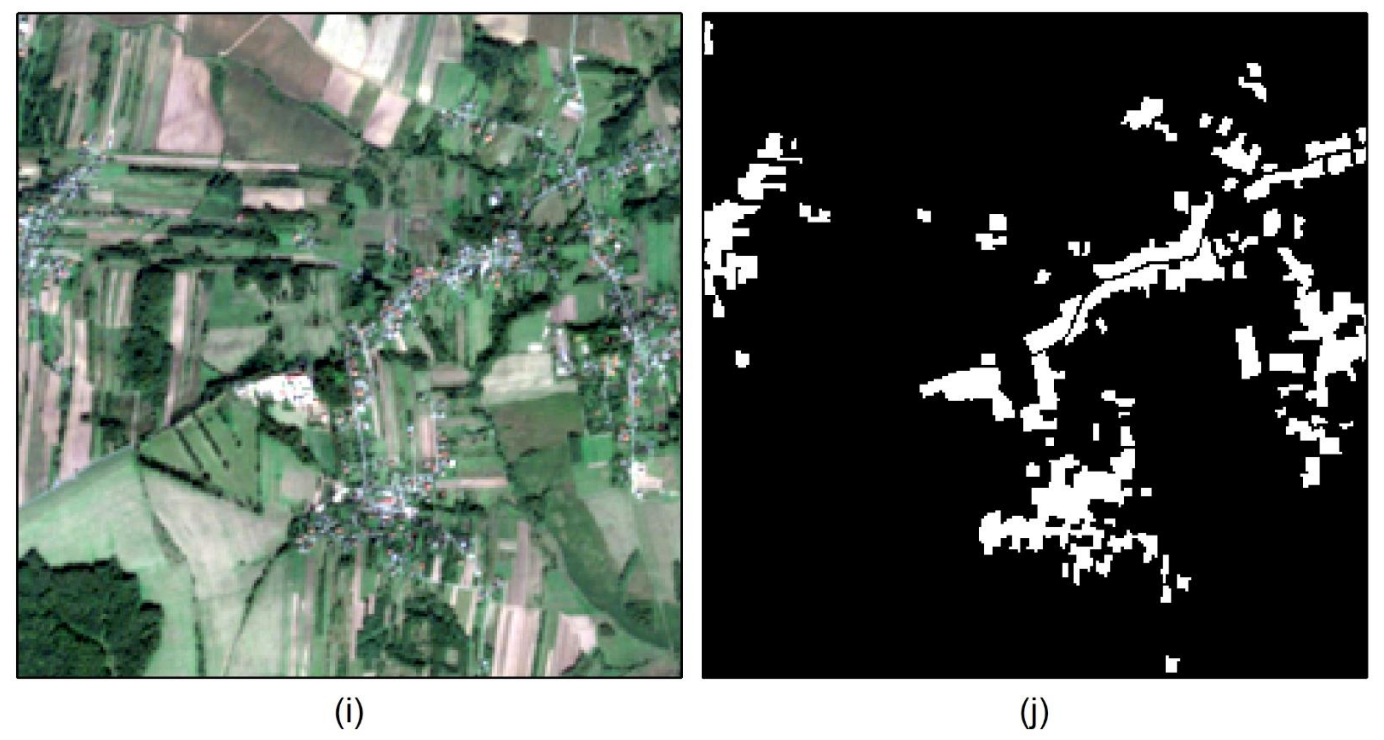
2.3. Methods of Analysis

The share of built-up areas cover within a given spatial unit area was calculated with the use of Sentinel-2 satellite images. In the first stage, a machine learning model was used to perform semantic segmentation and delineate built-up land cover. Then the obtained results were aggregated to the borders of the cities.

Semantic segmentation is a machine learning task of detecting a specific region of an image and assigning it a label to make this region distinguishable from different discovered regions and thus facilitating the process of image content interpretation [67]. Segmentation, in terms of the presented research, is a process of classifying pixels, originating from Sentinel-2 satellite images, into two categories representing built-up areas and other land cover types (Figure 2). The mask in supervised machine learning classification was representing built-up areas created by residential and industrial buildings, warehouse, agricultural production buildings, etc., together with small areas and devices, functionally related to buildings—such as yards, squares, court-yards, passages, crossings, home playgrounds, etc. [68].

The machine learning pipeline was prepared to support DeepLabV3+ [69] model using the Xception [70] backbone. The model has been implemented in Python 3.7 using Tensorflow 2.2.0 [71] and Keras 2.3.1 [72] frameworks. DeepLabV3+ is a deep convolutional neural network architecture characterized by its outstanding capabilities to handle the problem of segmenting objects at multiple scales by designing its main modules to capture multi-scale context. The use of other machine learning model architectures was also considered. During preliminary studies, such solutions as U-Net [73], FPN [74], and PSPNet [75] were tested but they showed less effectiveness than DeepLabV3+.

The model was trained using a loss function being a sum of binary focal loss [74] and Jaccard index loss [76]. During the process of model training, only the 2015 dataset was utilized. The 2015 dataset was the only one containing the area of the whole country and success in its correct segmentation was necessary to achieve satisfactory results in the 2019 dataset. The 2015 dataset was split into three subsets. The first subset intended for training accounted for 90% of the dataset. Validation subset was formed using 5% of the dataset. The main purpose of the validation subset was measuring the performance during intermediate training steps and for early stopping. Test data used during final model evaluation accounted for 5% of each set for 2015 and 2019. The accuracy of the model was monitored using the intersection over union (IoU), f1-score, pixel-wise binary accuracy, precision, and recall metrics. Foreground to background threshold was set to 0.5, meaning probability map values above 0.5 will be treated as built-up areas. Summary of evaluation on all datasets is presented in

Table 3. Summary of urban land cover semantic segmentation model evaluation on 2015 and 2019 datasets.

Dataset	IoU	F1-Score	Binary Accuracy	Precision	Recall
2015	0.548	0.708	0.979	0.693	0.726
2019	0.588	0.741	0.963	0.679	0.814

. Score values were calculated in relation to the ground truth segmentation mask, which had some flaws the model had to deal with. Although, the dataset used to produce segmentation maps is the largest and most precise source of information on built-up areas available in Poland, it is not free from defects. During careful analysis, one can discover that in multiple areas the delineated regions are visibly under or oversegmented. These issues were mitigated by crafting a model that is able to generalize well-enough to make the segmentation smoother. Overall, the model achieved satisfactory results, which was also indicated by the results of the perceptual evaluation.

It should be noted that the limitation of using the machine learning method to obtain data on built-up areas is the occurrence of cloud cover in satellite images used as source materials. The presence of cloud cover may limit or prevent the recognition of objects. However, the selection of cloudless satellite images or the use of cloud removal techniques makes this limitation quite easy to overcome [77,78,79].

The spatial diversity of cities in terms of the share of built-up areas in their area was analyzed using Geographic Information Systems (GIS) tools available in ArcGIS 10.7 software. Hot spot analysis using the Getis-Ord Gi* statistic was applied first [80,81,82]. It allows for finding statistically significant clusters of high (hot spots) and low values (cold spots) and is expressed by the formula:

$$G_i^{*}=\frac{{{\displaystyle \sum }}_{j=1}^n{w}_{i,j}{x}_j-\overline{X}{{\displaystyle \sum }}_{j=1}^n{w}_{i,j}}{S\sqrt{\frac{[n{{\displaystyle \sum }}_{j=1}^n{w}_{i,j}^2-{\left({{\displaystyle \sum }}_{j=1}^n{w}_{i,j}\right)}^2]}{n-1}}}$$

(1)

where x_j is the attribute value for feature j, w_i,j is the spatial weight between feature i and j, n is equal to the total number of feature and:

$$\overline{X}=\frac{{{\displaystyle \sum }}_{j=1}^n{x}_j}{n},$$

(2)

$$S=\sqrt{\frac{{{\displaystyle \sum }}_{j=1}^n{x}_j^2}{n}-{\left(\overline{X}\right)}^2}$$

(3)

The Getis-Ord Gi* local statistic score for each trait in the data set is the z-score. The occurrence of statistically significant positive z-scores indicates a hot spot. The larger the z-score, the more intense the clustering of high values. For statistically significant negative z-scores, there is a cold spot, the lower the score, the more intense the clustering of low values.

The use of GWR in the study was preceded by Ordinary Least Square (OLS), which aimed to identify the global spatially continuous influence of demographic, social, and economic factors on the share of built-up areas in the surface of small cities in Poland [49,83]. The OLS model is expressed as follows:

$$y_i={\beta }_0+{{\displaystyle \sum }}_{j=1}^n{\beta }_j{x}_{ij}+{\epsilon }_i,$$

(4)

where y_i is the observation of the dependent variable at location i, β₀ is a constant term, and β_j measures the relationship between independent variable x_ij and y for the set of i locations. ε_i is the error associated with location i.

GWR is an extension of global regression models and allows the estimation of local influences of demographic, social, and economic factors on the share of built-up area in small cities in Poland, the examination of spatial relationships between variables in the model and the identification of patterns [84,85,86]. The GWR model is expressed as follows:

$$y_i={\beta }_0\left(u_i,v_i\right)+{\displaystyle \sum }_{j=1}^n{\beta }_j(u_i,v_i)x_{ij}+{\epsilon }_i$$

(5)

where y_i is the dependent variable, i represents regions of the study area, (u_i, v_i) denotes the location of i observed region, βj(u_i, v_i) indicates the j regression parameter at the location of observation i, which is a function of the geographical position, x_ij is the independent variable, and ε_i is the random error of i region.

The results of GWR application were presented on a map showing the coefficient of determination describing the compatibility of local models with empirical observations and on maps estimating the values of the influence of local parameters of independent variables on the share of built-up area in the area of small cities in Poland and the significance of the identified impacts [87,88].

The procedure of data preparation and the processing steps were summarized in a schematic workflow given in Figure 3.

3. Results

3.1. Share of Built-Up Areas in the Area of Small Cities in Poland in 2019

Based on the data obtained as a result of machine learning segmentation of Sentinel-2 satellite images, the acreage of build-up areas was calculated for each city (Figure 4). Built-up areas were related to the area of each city within the administrative borders and the share of built-up areas in the urban area was determined.

The share of built-up areas in the urban area varies spatially. It can be indicated that cities with a low share of built-up areas are located mainly in southern Poland in the following regions: Śląski, Opolski, in the southern part of the Dolnośląski, and in the eastern part of the country in the Podlaski and on the border of the Świętokrzyski, Lubelski, and Podkarpacki (Figure 5). Cities with a high share of built-up areas were mainly located in Mazowiecki and Wielkopolski regions.

The analysis of the share of built-up areas in the area of small cities in Poland in 2019 also showed that the average share of built-up areas was 28.5% with a standard deviation of 0.99%. The lowest value of 1.7% was recorded for Krynica Morska, a city located in the north of Poland, in Pomorski region, on the Vistula Spit. The highest value, 83.6%, was recorded for the city of Łomianki, located in the Mazowiecki region and bordering Warsaw to the south. Cities with the lowest proportions of built-up areas, up to 15%, accounted for 20.6% of all cities surveyed. They were mainly located in the south and east of Poland. For 70.1% of the cities, the share of built-up areas ranged from 15 to 50%, while the highest shares of built-up areas in their area, above 50%, were found in 9.3% of the surveyed cities. They were mainly located in the central part of the Mazowiecki region, around the capital city of Warsaw, and in the western and southern parts of the Wielkopolski region (Figure 3).

3.2. Hot Spots and Cold Spots of the Share of Built-Up Areas in the Area of Small Cities in Poland in 2019

The applied Hot Spot analysis (Getis-Ord Gi*) allowed the identification of clusters of cities with a statistically significant high and low share of built-up areas in their area (Figure 6). There are two hot spots in the studied area, the first one in the central part of Mazowiecki region, in the area of Warsaw, the second, more extensive, covering Wielkopolski and Kujawsko-Pomorski regions. Cold spots occurred in three locations. The most extensive covered the southern part of Dolnośląski region, as well as Opolski and Śląski regions. The second was located on the border of three regions: Świętokrzyski, Mazowiecki, and Lubelski. The last cold spot was located in Podlaski region.

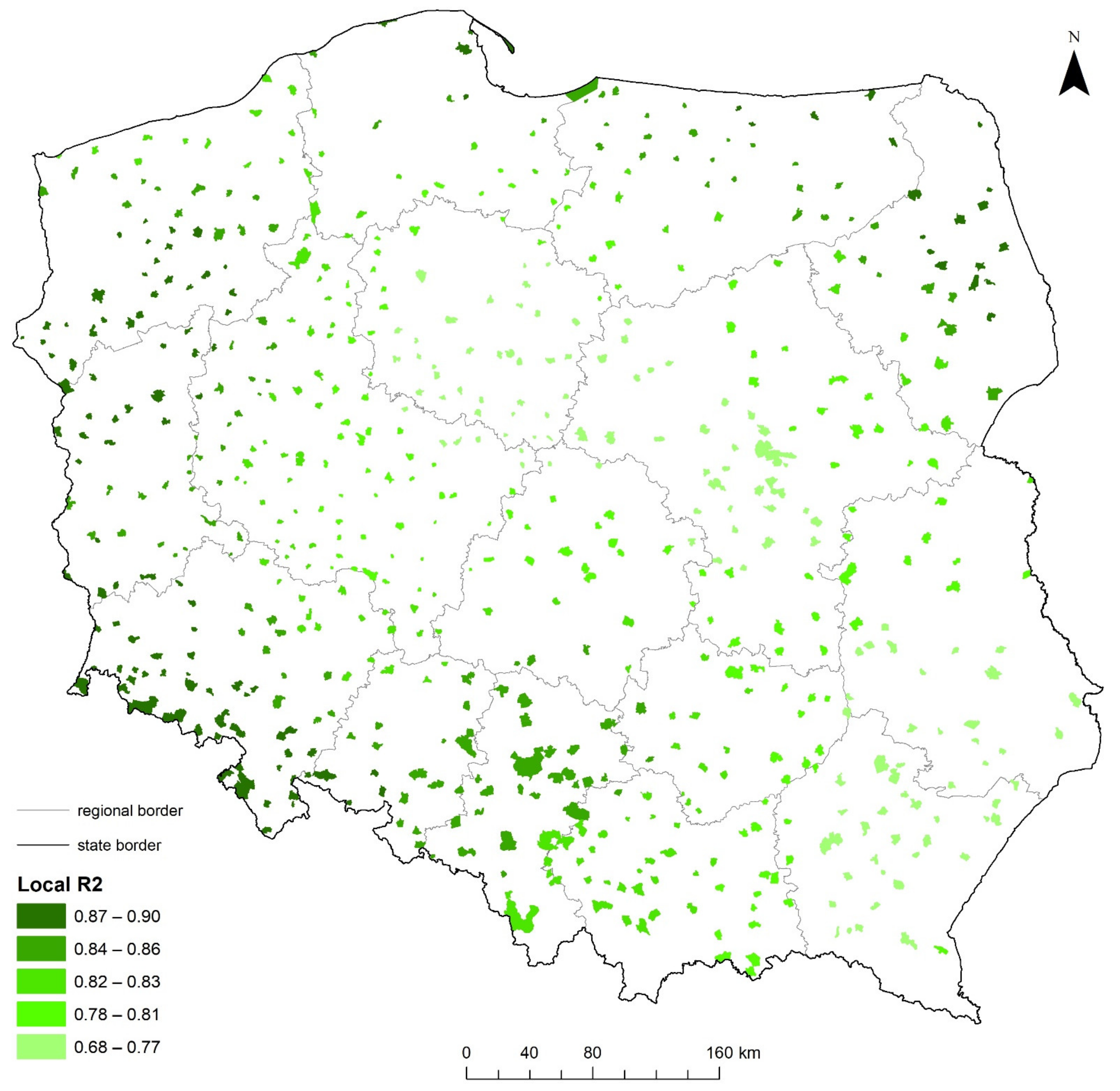
3.3. Global and Local Model of the Share of Built-Up Land in the Area of Small Cities in Poland

The global regression model (OLS) explaining the effect of selected variables on the share of built-up area in small cities in Poland in 2019 was evaluated (

Table 4. Global model estimating.

Variable	Coefficient	Standard Error	t−Value	p−Value
Pop_Density	0.9206	0.0207	44.4981	p−value < 0.01
Buildings	0.2014	0.0263	7.6640	p−value < 0.01
Unemployment	−0.0695	0.0185	−3.7638	p−value < 0.01
Work_Pop	−0.0311	0.0192	−1.6219	0.1565
Enterprises	−0.2115	0.0298	−7.1048	p−value < 0.01
Living_Standard	−0.0163	0.0204	−0.8027	0.4477

). The coefficient of determination for the global model (R²) reached 0.790, adjusted R² 0.788 and AICc (Akaike’s Information Criterion) equal to 863.971. This result can be regarded as satisfactory and pointing to significant associations between socio-economic variables and the share of built-up areas. All the more so, as four out of six variables were identified as statistically significant (p-value <0.01). Positive associations were noted for population density (Pop_Density) and the emergence of new residential buildings (Buildings). This may be caused by the increase in the wealth of the inhabitants and the need to improve housing conditions or the local development policy favoring the creation of new built-up areas. On the other hand, in cities with a higher unemployment (Unemployment) rate, the share of built-up areas in the area of the surveyed units is smaller. Interestingly, a negative association between the share of built-up areas in the surface area of small cities was shown for domestic economic entities (Enterprises).

For GWR, R² reached 0.868, adjusted R² 0.843 and AICc 713.881. Which indicates that the estimation of local models based on this method more effectively describes the phenomenon under study. Higher R² values indicate a stronger explanatory power of the regression model, and a model with a lower AICc value indicates a better fit to the observed data. GWR with Fixed Kernel type was used in the study because it achieved a smaller AICc compared to Adaptive Kernel type with an AICc of 717.095. The accuracy of GWR-based estimates of the local influence of various demographic social and economic factors on the share of built-up area in small cities in Poland varies spatially (Figure 7). The best estimates of the share of built-up areas according to the components under study were obtained for cities located in the Zachodniopomorski, Lubuski, and Dolnośląski regions occupying the western part of the country, and for cities from the Opolski and Śląski regions located in the south of Poland. This also applied to cities located in the north-east of Poland in the Podlaski and partly in the Warmińsko-Mazurski regions.

GWR coefficients for socio-economic factors describing the spatial variation of the share of built-up areas in the area of small cities (

Table 5. Summary of GWR coefficients depicting the spatially varying relationships between share of built-up areas in small cities [%] and socio-economic factors.

Socio−Economic Factors	Minimum	Median	Average	Maximum
Pop_Density	0.75	0.96	0.98	1.66
Buildings	0.03	0.18	0.21	1.02
Unemployment	−0.31	−0.09	−0.10	0.10
Work_Pop	−0.20	−0.02	−0.03	0.70
Enterprises	−0.65	−0.23	−0.24	0.01
Living_Standard	−0.20	−0.03	−0.03	0.11

) indicate positive associations between population density or the number of buildings in small cities and the share of built-up areas in the area of cities. The next two, the percentage of unemployed and the share of the population of working age, have a mostly negative associations with the examined characteristic. The most varied is the variable defining the quality of life of residents (defined by the share of bathrooms [%] in residential buildings), which takes both negative and positive values.

Population density (Pop_Density) was the most important spatial stimulant of the share of built-up areas in the area of the cities studied (Figure 8). The higher the population density, the greater the proportion of built-up areas. A significant relationship between population density and the share of built-up areas has been found for the whole of Poland. The strongest association with this variable was observed in the south of Poland in the following regions: Małopolski, Podkarpacki, and Świętokrzyski, and in the east of the country, in Lubelski and Podlaski. The weakest impact of this variable is seen in northern Poland in Pomorski, Kujawsko-Pomorski, and Warmińsko-Mazurski regions. As well as in the southern part of Dolnośląski and Opolski regions. These regions formed part of the cold spot of the share of built-up areas in the area of small cities (Figure 6) and are regions with an unfavorable economic structure, threatened by depopulation, which consequently also adversely affects the share of built-up areas in the area of small towns located within their borders.

A significant positive association was also found between the share of built-up areas in the area of small cities was also found in the number of new residential buildings put into use (Buildings) for a prevailing part of Poland, with the exception of Śląski, Małopolski, part of Lubelski, and Wielkopolski and Lubuski regions. This association was strongest in the northern part of Poland, in Pomorski and Zachodniopomorski regions, and partially in Warmińsko-Mazurski and Podlaski (Figure 9). This is an expected relationship, the construction of new buildings is an obvious cause of increasing the share of built-up areas in the area of the surveyed units. However, the lack of significance of this factor for the regions indicated above may mean that the buildings in the cities located there are relatively old and their large share in the area of the cities under study has been shaped by historical processes. This is particularly evident in the case of Wielkopolski region, where a hot spot of the share of built-up areas in the area of small cities is located (Figure 6).

A significant association was detected between the share of built-up areas in the area of small cities in Poland in 2019 was detected for the share of registered unemployed in the number of people of working age (Unemployment), mainly in the western and southern part of Poland, in Lubuski Wielkopolski, Dolnośląski Opolski and Śląski regions, as well as in the band stretching from the central part of Mazowiecki southwards through the western part of Lubelski to the northern part of Podkarpacki region (Figure 10). This association was mostly negative, meaning that the lower the unemployment rate, the higher the share of built-up areas in the area of the surveyed cities. The influence of this factor was strongest in southern Poland, in a belt running from the southern part of Lubuski, Dolnośląski, Opolski regions to the southern part of Śląski. The association with this variable can be seen in the occurrence of hot spots of the share of built-up areas in Wielkopolski and Mazowiecki regions (Figure 6), which were the areas with the lowest unemployment rate in Poland in 2019. It can as well be inferred that it has a partial influence on the occurrence of cold spots of the share of built-up areas in the area of small cities visible in the south of Poland, especially in Opolski and partly in Dolnośląski, which are regions at risk of depopulation and less development with higher unemployment.

Issues related to the share of working-age population in the total population (Work_Pop) are a predominantly negative factor associated with the share of built-up areas in the area of the surveyed cities. The smaller the share of the population of working age, the larger the share of built-up areas in the area of small cities. However, the impact of this variable is significant only for the central and northern part of Mazowiecki and the western part of Podlaski region (Figure 11). Although the impact of this variable is very limited, it can be concluded that it is related to the influence of the capital city of Warsaw, whose developed labor market attracts people of working age, especially from small cities located in its immediate and near vicinity.

Another variable—the number of newly registered domestic economic entities in the REGON register (Enterprises) had a significant association with the share of built-up areas in the area of small cities in the majority of the country, except for the regions located in the south of Poland: Opolski, Śląski, Małopolski, Podkarpacki, and partly Łódzki, Świętokrzyski, and Lubelski (Figure 12). The impact of this factor is overwhelmingly negative. The smaller the number of enterprises, the greater was the share of built-up areas in the area of the surveyed cities. This influence was strongest in the regions of western and northern Poland. From Dolnośląski region to the north through Zachodniopomorski to Podlaski region to the east. It can be assumed that buildings in these cities were mainly residential and newly registered domestic economic entities, e.g., services, were located in owners’ place of residence.

For the last examined variable, the quality of life expressed as the share of dwellings equipped with facilities (bathrooms) in the total number of dwellings (Living_Standard), two opposite statistically significant tendencies of association with the share of built-up area in small cities in Poland were observed (Figure 13). Negative relationship was observed in the belt running from Zachodniopomorski region, through Wielkopolski to the northern edges of Opolski and Śląski regions. In this area, the lower the quality of life, the higher the share of built-up area in the surveyed cities. An inverse relationship was found for the central part of Mazowiecki region, where a higher quality of life translates into a higher share of built-up areas in the area of small cities. Both areas coincide with the designated hot spots of the share of built-up areas in the area of the surveyed cities (Figure 6). These seemingly contradictory trends can be traced back to the different age of urban development in the two regions. While the buildings in cities centered around Warsaw, in the central part of the Mazowiecki region, have developed intensively over the last 25 years, the built-up areas in cities in Wielkopolski are relatively older and have been shaped by other historical factors, the conditions in which settlement units were established and developed throughout their existence.

The use of combined deep learning, Hot Spot analysis (Getis-Ord Gi*), and GWR methods allowed to identify the significance and impact of individual determinants. It was found that population density and the construction of new residential buildings had the greatest influence on the share of built-up areas in the area of the surveyed cities. The results also indicated that the share of built-up areas in the area of the cities under study is a result of the conditions under which they were established and developed, and not only of the socio-economic factors affecting them at present.

4. Discussion and Future Directions

The fact that cities are built up is not debatable, but the regional variation of the built-up areas suggests a need to examine the reasons and factors influencing this fact. The variables associated with the share of built-up areas in small cities in a national perspective have not yet been considered by researchers. A certain problem in determining the built-up areas in all cities in a given year is the lack of available up-to-date geodetic data sources. This is made possible by information extracted from satellite images [35,89,90,91]. The aim of this study was to investigate the spatial differentiation of the share of built-up areas in the area of small cities in Poland, as well as to search for factors influencing this differentiation. Sentinel-2 satellite images and data from the Statistics Poland were used for this purpose.

The paper is not able to make any causal claims, but the obtained results allowed for the identification of some statistically significant relationships between the studied variables. The scheme of the adopted research procedure has already been successfully applied in urban studies [49,50,63] The method of Hot Spot Analysis (Getis-Ord Gi*) was used to determine regional variations in the share of hot-spots and cold-spots in built-up areas (Figure 4). The GWR method was applied and it was found that the variables explaining the spatial variation in the share of built-up areas are regionally differentiated and have positive, negative, or mixed associations with the variable under study.

The variables used in the research were also applied in the other studies of small towns in Poland. The population related variable used most frequently was the number of inhabitants, population density, but also population dynamics and migrations. These variables often were the base for the selection of cities taken into account in the research, they were used to study the development of small towns and create a typology of settlement units [18,57,62,64]. Variables allowing to describe the economic activity of inhabitants of small cities in Poland were also often used. Data on professional activity, unemployment level, working age population, number of enterprises, or employment in a specific sector of the economy, e.g., in services, were used to study the development of small cities and the role they play in the country’s settlement system [1,57,64,92]. Variables related to the spatial development of small cities, such as changes in the administrative area of cities, share of urbanized area of the town, changes in the number of flats and houses, and infrastructure are used less frequently and mainly in the field of small town development [57,62]. The greatest differentiation occurs among the variables describing the living standards of small city residents. This issue can be described in various ways, often also through the subjective opinions of the inhabitants; however, the most frequently used in research are: the level of infrastructure development and access to services related to education, health, trade, and culture [1,16,92]. Positive associations with the share of built-up areas in small Polish cities have been detected for population density (Figure 8) and the number of new residential buildings (Figure 9). Negative relationships have been found for three socio-economic variables: the share of the registered unemployed in the working-age population (Figure 10), the share of working-age population in the total population (Figure 11), and—which was quite surprising—the number of newly registered domestic economic entities (Figure 12). The quality of life of inhabitants of small towns were determined with the use of the variable showing the share of dwellings equipped with facilities (bathrooms) in the total number of dwellings. This variable showed notable spatial differentiation and various associations (Figure 13). In the Mazowiecki region around Warsaw, it had a positive association with the share of built-up areas, but in Wielkopolski region the relationship was opposite. This indicates differences in the equipment of buildings forming built-up areas in the cities of these regions.

The inclusion of a temporal variable can not only improve inference but also reveal new relationships. In future research, the research area can be narrowed down to a single city or a group of cities, but it can also be extended to include a network of cities in Poland’s neighboring countries. Sentinel-2 satellite images offer this possibility. The issue to be resolved will be the selection of variables available for all the countries studied. Unfortunately, a major barrier is the lack of availability of statistical data. In the databases of Statistics Poland as well as Eurostat—European Statistics, most data are aggregated to the level of municipalities, which affects limited possibilities of statistical data analysis for small cities.

The presented research scheme may be an inspiration to undertake similar research. Capturing the relationship between the share of built-up areas and socio-economic factors requires further research. The proportion of built-up areas in cities is the result of long-standing processes and urban morphology. Most of the cities studied have medieval origins, but there are also those established during the industrialization of Poland, as well as tourist and spa towns, and others [93]. They play different roles in the Polish settlement system [1,92,94,95,96]. More and more towns in the suburban areas of large cities are growing rapidly in terms of population and built-up areas. As a consequence of this development, they will obtain city rights and change the urban settlement network of Poland. Others are going through economic stagnation or regression, with population declining and built-up areas remaining unchanged. It is worth continuing research with new variables and also their dynamics [97]. New variables can also be of a qualitative nature related to: the origins of cities, geographical location (lowlands, highlands, mountains), proximity to roads, transport hubs, ports, and large cities.

References

1. Czapiewski, K.; Bański, J.; Górczyńska, M. The Impact of Location on the Role of Small Towns in Regional Development: Mazovia, Poland. Eur. Countrys. 2016, 8, 413–426. [Google Scholar] [CrossRef] [Green Version]
2. Vaishar, A.; Št’astná, M.; Stonawská, K. Small Towns—Engines of Rural Development in the South-Moravian Region (Czechia): An Analysis of the Demographic Development. Acta Univ. Agric. Silvic. Mendel. Brun. 2015, 63, 1395–1405. [Google Scholar] [CrossRef] [Green Version]
3. Agergaard, J.; Kirkegaard, S.; Birch-Thomsen, T. Between Village and Town: Small-Town Urbanism in Sub-Saharan Africa. Sustainability 2021, 13, 1417. [Google Scholar] [CrossRef]
4. Tan, K.C. Small Towns in Chinese Urbanization. Geogr. Rev. 1986, 76, 265–275. [Google Scholar] [CrossRef]
5. Gu, C.; Li, Y.; Han, S.S. Development and Transition of Small Towns in Rural China. Habitat Int. 2015, 50, 110–119. [Google Scholar] [CrossRef]
6. Tan, M.; Li, X.; Xie, H.; Lu, C. Urban Land Expansion and Arable Land Loss in China—A Case Study of Beijing–Tianjin–Hebei Region. Land Use Policy 2005, 22, 187–196. [Google Scholar] [CrossRef]
7. Brennan, C.; Hackler, D.; Hoene, C. Demographic Change in Small Cities, 1990 to 2000. Urban Aff. Rev. 2005, 40, 342–361. [Google Scholar] [CrossRef]
8. Bell, D.; Jayne, M. Small Cities? Towards a Research Agenda. Int. J. Urban. Reg. Res. 2009, 33, 683–699. [Google Scholar] [CrossRef]
9. Demazière, C. Dealing with Small and Medium-Sized Towns (SMSTs) in Urban Studies. Espaces Sociétés 2017, 168–169, 17–32. [Google Scholar] [CrossRef] [Green Version]
10. Statistics Poland Local Data Bank. Available online: https://bdl.stat.gov.pl/BDL (accessed on 23 February 2021).
11. Demazière, C.; Serrano, J.; Vye, D. (Eds.) Introduction. Les villes petites et moyennes et leurs acteurs: Regards de chercheurs. In Villes Petites Et Moyennes (Norois); Presses Universitaires de Rennes: Rennes, France, 2012; pp. 7–10. [Google Scholar]
12. Knox, P.; Mayer, H. Small Town Sustainability: Economic, Social, and Environmental Innovation; Walter de Gruyter: Basel, Switzerland, 2013. [Google Scholar]
13. Mayer, H.; Knox, P. Small-Town Sustainability: Prospects in the Second Modernity. Eur. Plan Stud. 2010, 18, 1545–1565. [Google Scholar] [CrossRef]
14. Ahvenniemi, H.; Huovila, A.; Pinto-Seppä, I.; Airaksinen, M. What Are the Differences between Sustainable and Smart Cities? Cities 2017, 60, 234–245. [Google Scholar] [CrossRef]
15. Jażdżewska, I.; Frykowski, M. Rozwój gospodarczy gmin a aktywność obywatelska mieszkańców wsi i małych miast województwa łódzkiego. In Oblicza Kapitału Społecznego. Studium Teoretyczne i Empiryczne; Bylok, F., Kwiatek, A., Eds.; Politechnika Częstochowska Wydział Zarządzania: Częstochowa, Poland, 2009; pp. 71–84. [Google Scholar]
16. Kwiatek-Sołtys, A.; Mainet, H. Quality of Life and Attractiveness of Small Towns: A Comparison of France and Poland. Quaest. Geogr. 2014, 33, 103–113. [Google Scholar] [CrossRef] [Green Version]
17. Bell, D.; Jayne, M. Small Cities: Urban. Experience beyond the Metropolis; Routledge: London, UK, 2006. [Google Scholar]
18. Kamińska, W.; Mularczyk, M. Demographic Types of Small Cities in Poland. Misc. Geogr. 2014, 18, 24–33. [Google Scholar] [CrossRef] [Green Version]
19. Valtenbergs, V.; Ainhoa, G.; Ralfs, P. Selecting Indicators for Sustainable Development of Small Towns: The Case of Valmiera Municipality. Procedia Comput. Sci. 2013, 26, 21–32. [Google Scholar] [CrossRef] [Green Version]
20. Huovila, A.; Bosch, P.; Airaksinen, M. Comparative Analysis of Standardized Indicators for Smart Sustainable Cities: What Indicators and Standards to Use and When? Cities 2019, 89, 141–153. [Google Scholar] [CrossRef]
21. Nesticò, A.; Maselli, G. Sustainability Indicators for the Economic Evaluation of Tourism Investments on Islands. J. Clean. Prod. 2020, 248, 119217. [Google Scholar] [CrossRef]
22. Klusáková, L.; Ozouf-Marignier, M. Small Towns as European Cultural Heritage. Introduction. In Small Towns in Europe in the 20th and 21st Centuries; Klusáková, L., Ed.; Charles University in Prague, Karolinum Press: Prague, Czech Republic, 2017. [Google Scholar]
23. Van Lindert, P.; Verkoren, O. Small Towns and beyond: Rural Transformation and Small Urban Centres in Latin America; Thela Publishers: Amsterdam, The Netherlands, 1997. [Google Scholar]
24. Wisner, B.; Pelling, M.; Mascarenhas, A.; Holloway, A.; Ndong, B.; Faye, P.; Ribot, J.; Simon, D. Small cities and towns in Africa: Insights into adaptation challenges and potentials. In Urban Vulnerability and Climate Change in Africa; Springer: Berlin/Heidelberg, Germany, 2015; pp. 153–196. [Google Scholar]
25. Naikoo, M.W.; Rihan, M.; Ishtiaque, M.; Shahfahad. Analyses of Land Use Land Cover (LULC) Change and Built-up Expansion in the Suburb of a Metropolitan City: Spatio-Temporal Analysis of Delhi NCR Using Landsat Datasets. J. Urban Manag. 2020, 9, 347–359. [Google Scholar] [CrossRef]
26. Zhao, J.; Guo, W.; Huang, W.; Huang, L.; Zhang, D.; Yang, H.; Yuan, L. Characterizing Spatiotemporal Dynamics of Land Cover with Multi-Temporal Remotely Sensed Imagery in Beijing during 1978–2010. Arab. J. Geosci. 2013, 7, 3945–3959. [Google Scholar] [CrossRef]
27. Yin, J.; Yin, Z.; Zhong, H.; Xu, S.; Hu, X.; Wang, J.; Wu, J. Monitoring Urban Expansion and Land Use/Land Cover Changes of Shanghai Metropolitan Area during the Transitional Economy (1979–2009) in China. Environ. Monit. Assess. 2010, 177, 609–621. [Google Scholar] [CrossRef]
28. Yang, X.; Lo, C.P. Modelling Urban Growth and Landscape Changes in the Atlanta Metropolitan Area. Int. J. Geogr. Inf. Sci. 2003, 17, 463–488. [Google Scholar] [CrossRef]
29. Yang, X.; Lo, C.P. Using a Time Series of Satellite Imagery to Detect Land Use and Land Cover Changes in the Atlanta, Georgia Metropolitan Area. Int. J. Remote Sens. 2010, 23, 1775–1798. [Google Scholar] [CrossRef]
30. Yang, X.; Lo, C.P. Drivers of Land-Use/Land-Cover Changes and Dynamic Modeling for the Atlanta, Georgia Metropolitan Area. Photogramm. Eng. Remote Sens. 2002, 68, 1073–1082. [Google Scholar]
31. Yuan, F.; Sawaya, K.E.; Loeffelholz, B.C.; Bauer, M.E. Land Cover Classification and Change Analysis of the Twin Cities (Minnesota) Metropolitan Area by Multitemporal Landsat Remote Sensing. Remote Sens. Environ. 2005, 98, 317–328. [Google Scholar] [CrossRef]
32. Dewan, A.M.; Yamaguchi, Y. Using Remote Sensing and GIS to Detect and Monitor Land Use and Land Cover Change in Dhaka Metropolitan of Bangladesh during 1960–2005. Environ. Monit. Assess. 2008, 150, 237–249. [Google Scholar] [CrossRef] [PubMed]
33. Bagan, H.; Yamagata, Y. Land-Cover Change Analysis in 50 Global Cities by Using a Combination of Landsat Data and Analysis of Grid Cells. Environ. Res. Lett. 2014, 9, 1–13. [Google Scholar] [CrossRef]
34. Corbane, C.; Sabo, F.; Syrris, V.; Kemper, T.; Politis, P.; Pesaresi, M.; Soille, P.; Osé, K. Application of the Symbolic Machine Learning to Copernicus VHR Imagery: The European Settlement Map. IEEE Geosci. Remote Sens. Lett. 2020, 17, 1153–1157. [Google Scholar] [CrossRef]
35. Pesaresi, M.; Corbane, C.; Julea, A.; Florczyk, A.J.; Syrris, V.; Soille, P. Assessment of the Added-Value of Sentinel-2 for Detecting Built-Up Areas. Remote Sens. 2016, 8, 299. [Google Scholar] [CrossRef] [Green Version]
36. Haas, J.; Ban, Y. Sentinel-1A SAR and Sentinel-2A MSI Data Fusion for Urban Ecosystem Service Mapping. Remote Sens. Appl Soc. Environ. 2017, 8, 41–53. [Google Scholar] [CrossRef]
37. Liu, C.; Huang, X.; Zhu, Z.; Chen, H.; Tang, X.; Gong, J. Automatic Extraction of Built-Up Area from ZY3 Multi-View Satellite Imagery: Analysis of 45 Global Cities. Remote Sens. Environ. 2019, 226, 51–73. [Google Scholar] [CrossRef]
38. Weber, C.; Puissant, A. Urbanization Pressure and Modeling of Urban Growth: Example of the Tunis Metropolitan Area. Remote Sens. Environ. 2002, 86, 341–352. [Google Scholar] [CrossRef]
39. Zhou, W.; Troy, A.; Grove, M. Object-Based Land Cover Classification and Change Analysis in the Baltimore Metropolitan Area Using Multitemporal High Resolution Remote Sensing Data. Sensors 2008, 8, 1613–1636. [Google Scholar] [CrossRef] [Green Version]
40. McConnachie, M.M.; Shackleton, C.M. Public Green Space Inequality in Small Towns in South Africa. Habitat Int. 2010, 34, 244–248. [Google Scholar] [CrossRef] [Green Version]
41. Gismalla, Y.A.; Bruen, M. Use of a GIS in Reconnaissance Studies for Small-Scale Hydropower Development in a Developing Country: A Case Study from Tanzania. IAHS Publ. Ser. Proc. Rep. Intern Assoc. Hydrol. Sci. 1996, 235, 307–312. [Google Scholar]
42. Weng, Q. Modeling Urban Growth Effects on Surface Runoff with the Integration of Remote Sensing and GIS. Environ. Manag. 2001, 28, 737–748. [Google Scholar] [CrossRef]
43. Wright, J.; Liu, J.; Bain, R.; Perez, A.; Crocker, J.; Bartram, J.; Gundry, S. Water Quality Laboratories in Colombia: A GIS-Based Study of Urban and Rural Accessibility. Sci. Total. Environ. 2014, 485–486, 643–652. [Google Scholar] [CrossRef]
44. Stoica, I.-V.; Tulla, A.F.; Zamfir, D.; Petrișor, A.-I. Exploring the Urban Strength of Small Towns in Romania. Soc. Indic. Res. 2020, 152, 843–875. [Google Scholar] [CrossRef]
45. Cieślak, I.; Biłozor, A.; Szuniewicz, K. The Use of the CORINE Land Cover (CLC) Database for Analyzing Urban Sprawl. Remote Sens. 2020, 12, 282. [Google Scholar] [CrossRef] [Green Version]
46. Li, S.; Zhou, C.; Wang, S.; Gao, S.; Liu, Z. Spatial Heterogeneity in the Determinants of Urban Form: An Analysis of Chinese Cities with a GWR Approach. Sustainability 2019, 11, 479. [Google Scholar] [CrossRef] [Green Version]
47. Bitter, C.; Mulligan, G.F.; Dall’erba, S. Incorporating Spatial Variation in Housing Attribute Prices: A Comparison of Geographically Weighted Regression and the Spatial Expansion Method. J. Geogr. Syst. 2007, 9, 7–27. [Google Scholar] [CrossRef] [Green Version]
48. Ganguly, K.; Kumar, R.; Reddy, K.M.; Rao, P.J.; Saxena, M.R.; Shankar, G.R. Optimization of Spatial Statistical Approaches to Identify Land Use/Land Cover Change Hot Spots of Pune Region of Maharashtra Using Remote Sensing and GIS Techniques. Geocarto Int. 2017, 32, 777–796. [Google Scholar] [CrossRef]
49. Zhao, F.; Tang, L.; Qiu, Q.; Wu, G. The Compactness of Spatial Structure in Chinese Cities: Measurement, Clustering Patterns and Influencing Factors. Ecosyst. Health Sustain. 2020, 6, 1743763. [Google Scholar] [CrossRef] [Green Version]
50. Ivajnšič, D.; Kaligarič, M.; Žiberna, I. Geographically Weighted Regression of the Urban Heat Island of a Small City. Appl. Geogr. 2014, 53, 341–353. [Google Scholar] [CrossRef]
51. Brunsdon, C.; Fotheringham, A.S.; Charlton, M.E. Geographically Weighted Regression: A Method for Exploring Spatial Nonstationarity. Geogr. Anal. 1996, 28, 281–298. [Google Scholar] [CrossRef]
52. Gao, J.; Li, S. Detecting Spatially Non-Stationary and Scale-Dependent Relationships between Urban Landscape Fragmentation and Related Factors Using Geographically Weighted Regression. Appl. Geogr. 2011, 31, 292–302. [Google Scholar] [CrossRef]
53. Royuela, V.; Moreno, R.; Vayá, E. Influence of Quality of Life on Urban Growth: A Case Study of Barcelona, Spain. Reg. Stud. 2010, 44, 551–567. [Google Scholar] [CrossRef] [Green Version]
54. Bagan, H.; Yamagata, Y. Analysis of Urban Growth and Estimating Population Density Using Satellite Images of Nighttime Lights and Land-Use and Population Data. GISci. Remote Sens. 2015, 52, 765–780. [Google Scholar] [CrossRef]
55. Noresah, M.S.; Ruslan, R. Modelling Urban Spatial Structure Using Geographically Weighted Regression. In Proceedings of the 18th World IMACS Congress and MODSIM09 International Congress on Modelling and Simulation, The Australian National University Canberra, Cairns, QLD, Australia, 13–17 July 2009. [Google Scholar]
56. Shariff, N.M.; Gairola, S.; Talib, A. Modelling Urban Land Use Change Using Geographically Weighted Regression and the Implications for Sustainable Environmental Planning. In Proceedings of the 5th Biennial Conference of the International Environmental Modelling and Software Society, iEMSs 2010, Ottawa, ON, Canada, 5–8 July 2010. [Google Scholar]
57. Kwiatek-Sołtys, A. Small Towns in Poland-Barriers and Factors of Growth. Procedia Soc. Behav. Sci. 2011, 19, 363–370. [Google Scholar] [CrossRef] [Green Version]
58. Jażewicz, I. Rola Małych Miast w Przestrzeni Rolniczej Pomorza Środkowego. Studia Obsz. Wiej. 2006, 11, 159–172. [Google Scholar]
59. Jażewicz, I. Przemiany Społeczno-Demograficzne i Gospodarcze w Małych Miastach Pomorza Środkowego w Okresie Transformacji Gospodarczej. Słupskie Pr. Geogr. 2005, 2, 71–79. [Google Scholar]
60. Han, S.S. Urban Expansion in Contemporary China: What Can We Learn from a Small Town? Land Use Policy 2010, 27, 780–787. [Google Scholar] [CrossRef]
61. White, A. Informal Practices, Unemployment, and Migration in Small-Town Poland. East. Eur. Politics Soc. 2015, 30, 404–422. [Google Scholar] [CrossRef]
62. Parysek, J.J. Development of Polish Towns and Cities and Factors Affecting this Process at the Turn of the Century. Geogr. Pol. 2005, 78, 99–115. [Google Scholar]
63. Nilsson, P. Natural Amenities in Urban Space–A Geographically Weighted Regression Approach. Landsc. Urban Plan. 2014, 121, 45–54. [Google Scholar] [CrossRef]
64. Zuzańska-Żyśko, E. Economic Transformation of Small Silesian Towns in the Years 1990–1999. Geogr. Pol. 2005, 78, 136–149. [Google Scholar]
65. Wear, D.N.; Bolstad, P. Land-Use Changes in Southern Appalachian Landscapes: Spatial Analysis and Forecast Evaluation. Ecosystems 1998, 1, 575–594. [Google Scholar] [CrossRef] [Green Version]
66. Handavu, F.; Chirwa, P.W.C.; Syampungani, S. Socio-Economic Factors Influencing Land-Use and Land-Cover Changes in the Miombo Woodlands of the Copperbelt Province in Zambia. For. Policy Econ. 2019, 100, 75–94. [Google Scholar] [CrossRef] [Green Version]
67. Adamiak, M.; Biczkowski, M.; Leśniewska-Napierala, K.; Nalej, M.; Napierala, T. Impairing Land Registry: Social, Demographic, and Economic Determinants of Forest Classification Errors. Remote Sens. 2020, 12, 2628. [Google Scholar] [CrossRef]
68. In 1642 Rozporządzenie Ministra Spraw Wewnętrznych i Administracji z Dnia 17 Listopada 2011r. w Sprawie Bazy Danych Obiektów Topograficznych Oraz Bazy Danych Obiektów Ogólnogeograficznych, a Także Standardowych Opracowań Kartograficznych. In Dz.U. 2011 nr 279 poz.; The President of the Council of Ministers: Warsaw, Poland, 2011; Volume 279, pp. 16096–16099.
69. Chen, L.-C.; Papandreou, G.; Schroff, F.; Adam, H. Rethinking Atrous Convolution for Semantic Image Segmentation. arXiv 2017, arXiv:1706.05587. [Google Scholar]
70. Chollet, F. Xception: Deep Learning with Depthwise Separable Convolutions. In Proceedings of the IEEE Conference on Computer Vision and Pattern Recognition, Honolulu, HI, USA, 21 July 2017; pp. 1251–1258. [Google Scholar]
71. TensorFlow. Available online: https://www.tensorflow.org/ (accessed on 30 January 2021).
72. Lin, T.-Y.; Dollár, P.; Girshick, R.; He, K.; Hariharan, B.; Belongie, S. Feature Pyramid Networks for Object Detection. In Proceedings of the IEEE Conference on Computer Vision and Pattern Recognition, Honolulu, HI, USA, 21–26 July 2017; pp. 2117–2125. [Google Scholar]
73. Ronneberger, O.; Fischer, P.; Brox, T. U-Net: Convolutional Networks for Biomedical Image Segmentation. In Proceedings of the International Conference on Medical Image Computing and Computer-Assisted Intervention, Munich, Germany, 5–9 October 2015; pp. 234–241. [Google Scholar]
74. Lin, T.-Y.; Goyal, P.; Girshick, R.; He, K.; Dollár, P. Focal Loss for Dense Object Detection. In Proceedings of the IEEE International Conference on Computer Vision, Venice, Italy, 22–29 October 2017; pp. 2980–2988. [Google Scholar]
75. Zhao, H.; Shi, J.; Qi, X.; Wang, X.; Jia, J. Pyramid Scene Parsing Network. In Proceedings of the IEEE Conference on Computer Vision and Pattern Recognition, Honolulu, HI, USA, 26 July 2017; pp. 2881–2890. [Google Scholar]
76. Bertels, J.; Eelbode, T.; Berman, M.; Vandermeulen, D.; Maes, F.; Bisschops, R.; Blaschko, M.B. Optimizing the Dice Score and Jaccard Index for Medical Image Segmentation: Theory and Practice. In Proceedings of the International Conference on Medical Image Computing and Computer-Assisted Intervention, Shenzhen, China, 13–17 October 2019; pp. 92–100. [Google Scholar]
77. Shen, H.; Li, H.; Qian, Y.; Zhang, L.; Yuan, Q. An Effective Thin Cloud Removal Procedure for Visible Remote Sensing Images. ISPRS J. Photogramm. Remote Sens. 2014, 96, 224–235. [Google Scholar] [CrossRef]
78. Gao, J.; Yuan, Q.; Li, J.; Zhang, H.; Su, X. Cloud Removal with Fusion of High Resolution Optical and SAR Images Using Generative Adversarial Networks. Remote Sens. 2020, 12, 191. [Google Scholar] [CrossRef] [Green Version]
79. Meraner, A.; Ebel, P.; Zhu, X.X.; Schmitt, M. Cloud Removal in Sentinel-2 Imagery Using a Deep Residual Neural Network and SAR-Optical Data Fusion. ISPRS J. Photogramm. Remote Sens. 2020, 166, 333–346. [Google Scholar] [CrossRef] [PubMed]
80. Getis, A. Spatial Autocorrelation. In Handbook of Applied Spatial Analysis; Fischer, M.M., Getis, A., Eds.; Springer: Berlin, German, 2010; pp. 255–278. [Google Scholar]
81. Anselin, L.; Getis, A. Spatial Statistical Analysis and Geographic Information Systems. Ann. Reg. Sci. 1992, 26, 19–33. [Google Scholar] [CrossRef]
82. Ord, J.K.; Getis, A. Local Spatial Autocorrelation Statistics: Distributional Issues and an Application. Geogr. Anal. 1995, 27, 286–306. [Google Scholar] [CrossRef]
83. Brown, D.G.; Duh, J.-D. Spatial Simulation for Translating from Land Use to Land Cover. Int. J. Geogr. Inf. Sci. 2004, 18, 35–60. [Google Scholar] [CrossRef]
84. Fotheringham, A.S.; Brunsdon, C.; Charlton, M. Geographically Weighted Regression: The Analysis of Spatially Varying Relationships; John Wiley & Sons: Chichester, UK, 2002. [Google Scholar]
85. Brunsdon, C.; Fotheringham, A.S.; Charlton, M. Some Notes on Parametric Significance Tests for Geographically Weighted Regression. J. Reg. Sci. 1999, 39, 497–524. [Google Scholar] [CrossRef]
86. Brunsdon, C.; Fotheringham, S.; Charlton, M. Geographically Weighted Regression as a Statistical Model; University of Newcastle-upon-Tyne: Newcastle, UK, 2000. [Google Scholar]
87. Matthews, S.A.; Yang, T.C. Mapping the Results of Local Statistics: Using Geographically Weighted Regression. Demogr. Res. 2012, 26, 151–166. [Google Scholar] [CrossRef] [Green Version]
88. Mennis, J. Mapping the Results of Geographically Weighted Regression. Cartogr. J. 2006, 43, 171–179. [Google Scholar] [CrossRef] [Green Version]
89. Corbane, C.; Syrris, V.; Sabo, F.; Politis, P.; Melchiorri, M.; Pesaresi, M.; Soille, P.; Kemper, T. Convolutional Neural Networks for Global Human Settlements Mapping from Sentinel-2 Satellite Imagery. Neural Comput. Appl. 2020, 1–24. [Google Scholar] [CrossRef]
90. Ettehadi Osgouei, P.; Kaya, S.; Sertel, E.; Alganci, U. Separating Built-Up Areas from Bare Land in Mediterranean Cities Using Sentinel-2A Imagery. Remote Sens. 2019, 11, 345. [Google Scholar] [CrossRef] [Green Version]
91. Sinha, P.; Verma, N.K.; Ayele, E. Urban Built-up Area Extraction and Change Detection of Adama Municipal Area Using Time-Series Landsat Images. Int. J. Adv. Remote Sens. GIS 2016, 5, 1886–1895. [Google Scholar] [CrossRef]
92. Konecka-Szydłowska, B.; Zuzańska-Żyśko, E.; Szmytkie, R. Role of Services in the Economies of Small Towns of Silesia Region and Wielkopolskie Voivodehip. Bull. Geogr. Socio Econ. Ser. 2010, 14, 51–62. [Google Scholar] [CrossRef] [Green Version]
93. Jażdżewska, I. Urban Network in Poland during Last Millennium. Konwersatorium Wiedzy Mieście 2020, 5, 7–20. [Google Scholar] [CrossRef]
94. Kobojek, E.; Marszał, T. Local development and the role of small towns in space organisation in contemporary Poland. In Spatial Development of Contemporary Poland in Łódź University Geographical Rersearch; Marszał, T., Ed.; Łódź University Press: Łódź, Poland, 2014; pp. 37–60. [Google Scholar]
95. Lamprecht, M. Small Towns and Development of Rural Areas: The Case of the Voivodship of Łódź. Eur. Spat. Res. Policy 2004, 11, 41–56. [Google Scholar]
96. Jażdżewska, I. Rola małych miast w miejskiej sieci osadniczej Polski. In Podstawy i Perspektywy Rozwoju Małych Miast; Rydz, E., Ed.; Akademia Pomorska w Słupsku: Słupsk, Poland, 2007; pp. 31–46. [Google Scholar]
97. Shubho, M.T.H.; Islam, I. An Integrated Approach to Modeling Urban Growth Using Modified Built-Up Area Extraction Technique. Int. J. Environ. Sci. Technol. 2020, 17, 1–18. [Google Scholar] [CrossRef]
Figure 1. Cities in Poland by population in 1999 based on Head Office of Geodesy and Cartography (GUGiK) borders register and Statistics Poland data.
Geosciences 11 00223 g001
Figure 2. Examples of images (a,c,e,g,i) and segmentation maps (b,d,f,h,j).
Geosciences 11 00223 g002aGeosciences 11 00223 g002bGeosciences 11 00223 g002c
Figure 3. Methodology flowchart for analysis of built-up areas of small Polish cities in 2019 with the use of deep learning and geographically weighted regression.
Geosciences 11 00223 g003
Figure 4. Build-up areas obtained as a result of machine learning segmentation, examples of: (a) Nieszawa (b) Ujście, (c) Nowogród Bobrzański, (d) Pilawa, (e) Sośniowice, (f) Ustka, (g) Olecko, (h) Sobótka, (i) Nowogard, (j) Głowno.
Geosciences 11 00223 g004aGeosciences 11 00223 g004bGeosciences 11 00223 g004c
Figure 5. Share of built-up areas in the administrative area of small cities in Poland in 2019.
Geosciences 11 00223 g005
Figure 6. Hot spots of share of built-up areas in the administrative area of cities in 2019.
Geosciences 11 00223 g006
Figure 7. Coefficients of determination of local models estimating share of built-up areas in the area of small Polish cities in 2019.
Geosciences 11 00223 g007
Figure 8. Value (a) and significance (b) of the coefficient of the effect of population density (Pop_Density) on the share of built-up land in the area of Polish small cities in 2019.
Geosciences 11 00223 g008
Figure 9. Value (a) and significance (b) of the coefficient of the effect of the number of new residential buildings put into use (Buildings) on the share of built-up area in the area of small Polish cities in 2019.
Geosciences 11 00223 g009
Figure 10. Value (a) and significance (b) of the coefficient of the impact of the share of registered unemployed in the number of people of working age (Unemployment) on the share of built-up areas in the area of Polish cities in 2019.
Geosciences 11 00223 g010
Figure 11. Value (a) and significance (b) of the coefficient of the impact of the share of working-age population in the total population (Work_Pop) on the share of built-up land in the area of small Polish cities in 2019.
Geosciences 11 00223 g011
Figure 12. Value (a) and significance (b) of the coefficient of the impact of newly registered domestic economic entities in the REGON register (Enterprises) on the share of built-up areas in the area of small cities in Poland in 2019.
Geosciences 11 00223 g012
Figure 13. Value (a) and significance (b) of the coefficient of the impact of the share of dwellings equipped with facilities (bathrooms) in the total number of dwellings (Living_Standard) on the share of built-up areas in the area of small cities in Poland in 2019.
Geosciences 11 00223 g013