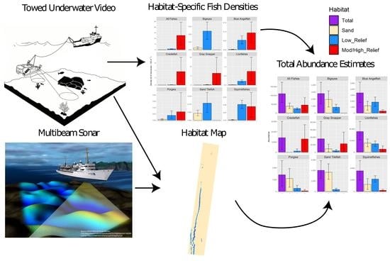
Integrating Towed Underwater Video and Multibeam Acoustics for Marine Benthic Habitat Mapping and Fish Population Estimation

Abstract

The west Florida shelf (WFS; Gulf of Mexico, USA) is an important area for commercial and recreational fishing, yet much of it remains unmapped and unexplored, hindering effective monitoring of fish stocks. The goals of this study were to map the habitat at an intensively fished area on the WFS known as “The Elbow”, assess the differences in fish communities among different habitat types, and estimate the abundance of each fish taxa within the study area. High-resolution multibeam bathymetric and backscatter data were combined with high-definition (HD) video data collected from a near-bottom towed vehicle to characterize benthic habitat as well as identify and enumerate fishes. Two semi-automated statistical classifiers were implemented for obtaining substrate maps. The supervised classification (random forest) performed significantly better (p = 0.001; α = 0.05) than the unsupervised classification (k-means clustering). Additionally, we found it was important to include predictors at a range of spatial scales. Significant differences were found in the fish community composition among the different habitat types, with both substrate and vertical relief found to be important with rock substrate and higher relief areas generally associated with greater fish density. Our results are consistent with the idea that offshore hard-bottom habitats, particularly those of higher vertical relief, serve as “essential fish habitat”, as these rocky habitats account for just 4% of the study area but 65% of the estimated total fish abundance. However, sand contributes 35% to total fish abundance despite comparably low densities due to its large area, indicating the importance of including these habitats in estimates of abundance as well. This work demonstrates the utility of combining towed underwater video sampling and multibeam echosounder maps for habitat mapping and estimation of fish abundance.

1. Introduction

Mapping of benthic habitats has become a critical element of living marine resource management globally [1,2,3,4]. Detailed habitat maps, at spatial scales relevant to management actions, provide the basis for protecting sensitive biota that may be vulnerable to disruptive human activities [5] and for evaluating the relationships of abundance and community structure of plants and animals to particular habitat types. Marine spatial planning, an element of ecosystem-based management, requires detailed, georeferenced information on benthic sediment types, and ecological processes within them [1,3,5,6]. In order to meet the demand for broad scale, accurate, and timely habitat mapping products, a variety of technologies and protocols have been developed and tested [7,8,9]. However, most of these technologies do not individually provide comprehensive, synoptic, or relatively unambiguous interpretations of habitat features and their biotic attributes.

Benthic habitat mapping generally involves performing an acoustic survey (e.g., with a multibeam echosounder) over a region of interest with systematic transects of data derived via “mowing the lawn” [10,11]. For a multibeam echosounder (MBES), the width of individual transects and thus the efficiency of such sequential approaches are dictated primarily by water depth. MBES provides a detailed topography (bathymetry) product plus a backscatter image which measures the intensity of the returning sound pulse and can be indicative of sediment grain size, composition, and substrate type [10,11,12,13,14,15,16]. In addition, ground-truthing data, for example, collected from camera imagery, must be collected in order to inform or verify interpretations of the acoustic returns and understand what sediment and other geological features they represent and to identify the biota associated with these habitats [7,8,17]. Additionally, with the increasing volume of data and the greater demand for habitat maps for ecosystem-based management and marine spatial planning, scientists and managers must consider the reliability of MBES data and their derivative metrics as surrogates to classify habitat types over differing spatial scales, especially where no independent ground-truthing exists [9,17,18,19,20,21]. For bathymetry, these derivative features include terrain attributes such as slope, rugosity, aspect, etc. [21,22], and for backscatter, these include texture metrics such as those derived from a gray level co-occurrence matrix (GLCM) [23,24,25,26,27,28,29].

Benthic habitat maps have the potential to make significant contributions to fisheries science. For example, habitat maps in the Florida Keys (USA) have facilitated habitat-stratified surveys, leading to more precise and cost-effective fisheries-independent monitoring surveys [30], which have become more important for monitoring as stricter management regulations have reduced the data available from fisheries-dependent sources [31,32,33,34]. Although the west Florida shelf (WFS; Gulf of Mexico, USA) is an important commercial and recreational fishing area, much of the WFS remains unmapped and unexplored, hindering effective monitoring of fish stocks [34,35,36]. Additionally, fisheries are typically managed using relative indices of abundance; however, what is of interest to managers are absolute estimates of abundance [37,38,39] when species are managed under an overall catch quota.

In this study, we demonstrate how MBES and towed underwater video can be used in tandem to extrapolate a small video sub-sample to provide predicted habitat maps for the entire study area and estimate absolute fish abundance in a popular fishing area on the WFS known as “The Elbow”. We compare the performance of two different approaches for mapping habitat: a supervised approach (random forest) and an unsupervised approach (k-means clustering) [10]. Additionally, we investigate the importance of predictors derived from different sources (bathymetry vs. backscatter) and over several spatial scales of analysis in the mapping procedure. Moreover, we test if the fish communities differ significantly among habitat types and identify the taxa driving any differences. Lastly, we demonstrate how these habitat maps can be combined with fish density data from a towed video survey to estimate fish abundance.

2. Materials and Methods

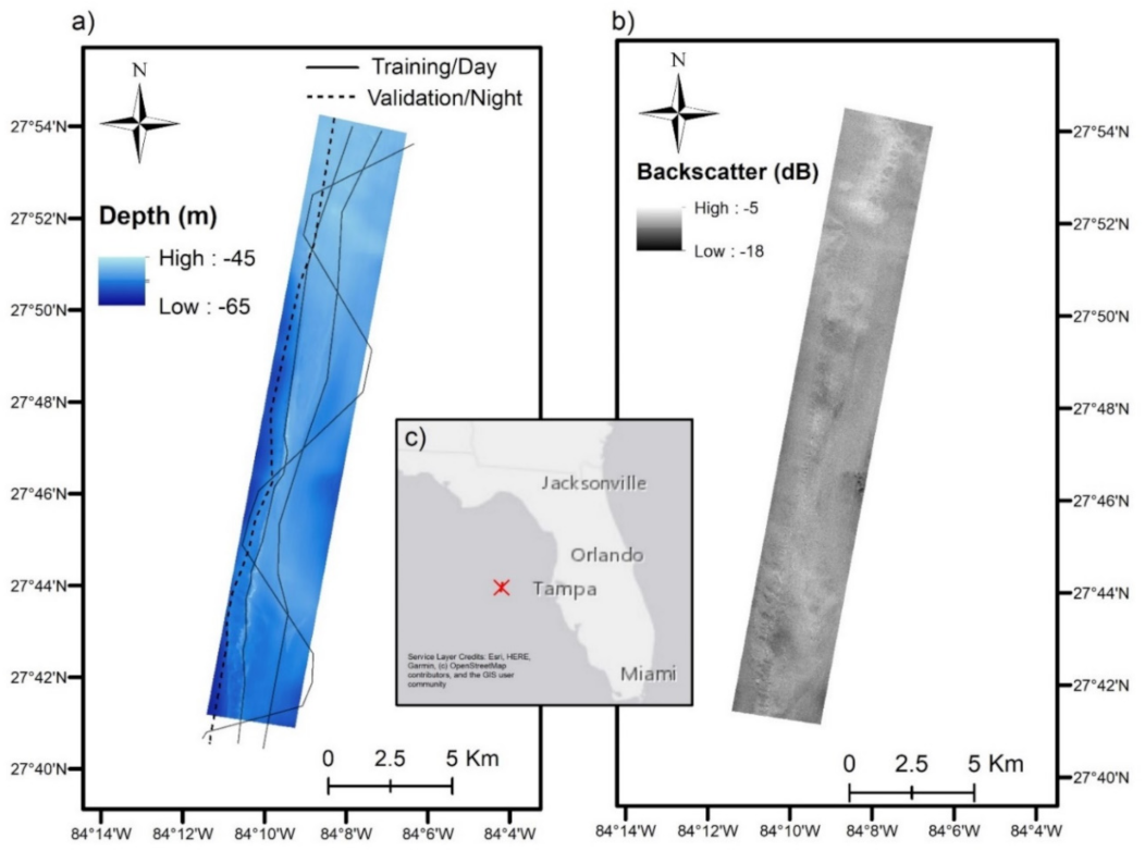
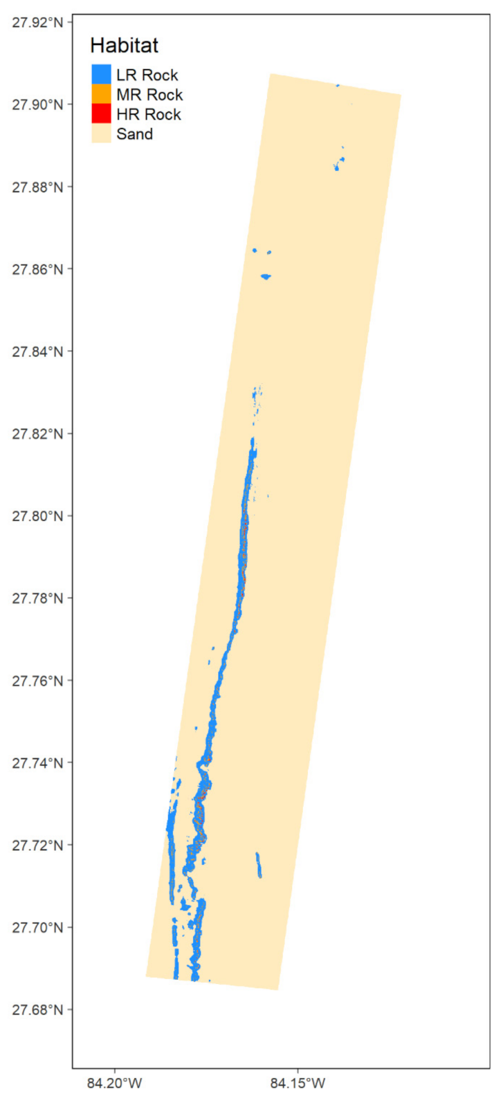
2.1. Study Area

The Elbow is hypothesized to be an ancient sea level stand shaped by wave action approximately 12,000 years ago [36,40]. The area lies 145 km west-northwest of Tampa Bay, Florida (Figure 1). It contains both hard-bottom (rock) and soft-bottom (sand) habitats, supporting associated benthic invertebrate assemblages including sponges, gorgonians, and sea urchins as well as a diverse community of reef fishes. The portion of the Elbow surveyed in this study (see next section) ranged in depth from 45 m to 65 m and contains a linear ridge that runs north to south for 16 km (Figure 1a). This area was chosen as a candidate to test and develop this analysis protocol for integrating towed video and MBES data because the hard-bottom ridges formed by paleo-shorelines in this area are representative of what we would expect elsewhere on the WFS [41]. Additionally, vessel monitoring systems (i.e., satellite tracking) data have identified the Elbow as a reef fishing “hot spot” [42,43], and this area is of interest to fisheries management [34,36].

2.2. Data Collection and Processing

2.2.1. Multibeam Echosounder Data

In December of 2015, 88 km² of the Elbow region was surveyed using a Teledyne Reson SeaBat 7125 MBES (Figure 1). This echosounder has 512 overlapping beams and was operated at 400 kHz with a 140° swath. The SeaBat 7125 was pole-mounted on the port side of the R/V Bellows operated by the Florida Institute of Oceanography. Navigation and motion compensation data were collected with an Applanix POS MV OceanMaster system [44]. An AML Oceanographic Micro•X was used to correct for sound launch velocity at the sonar head, and an AML Oceanographic Minos•X with an SV•Xchange sound velocity sensor was used for sound velocity profile correction to compensate for changes in the speed of sound throughout the water column.

Bathymetry data were post-processed using Caris HIPS and SIPS 10.2 with depth uncertainties less than 0.35 m [45]. The backscatter mosaic was created using the Caris SIPS time series algorithm. The bathymetry surface and the backscatter mosaic were exported to 2 m × 2 m resolution and 1 m × 1 m resolution raster grids, respectively. The bathymetry surface was then aggregated to a coarser 10 m × 10 m resolution grid, and the backscatter was aligned to a matching grid using bilinear interpolation so that both surfaces were referenced to a common grid as required for use in the statistical substrate habitat models (Figure 1). A resolution of 10 m × 10 m was chosen, as this approximates the scale of video observations, reduces artifacts in terrain attributes, and reduces potential errors related to positional uncertainty of the towed video system.

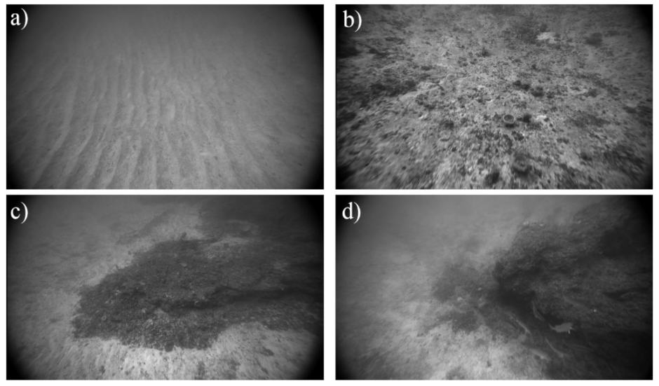
2.2.2. Towed Underwater Video

The Camera-Based Assessment Survey System (C-BASS) is a towed underwater camera system custom built to non-lethally sample demersal reef fish and classify bottom types [46,47]. The C-BASS is towed behind a research vessel at speeds of 1.5–2 m s⁻¹ and between 2–4 m above the seafloor [46]. The system consists of four LED lights and six underwater video cameras [46,47]. All cameras on the C-BASS are oriented obliquely at a downward angle from the main horizontal chassis, as this increases the area observed, increases fish detection probability, and provides a perspective that aids in the simultaneous identification of fish species and associated habitat characteristics [47,48]. A forward-facing monochrome HD camera was used as the primary camera to identify fish and habitat types in this study, as it consistently provided the clearest imagery, however, other color onboard cameras were used to aid in identification of fish and habitats. This primary camera is a FLIR Blackfly Gige Vision camera with a Sony IMX249 image sensor (13.3 mm diagonal; 1920 × 1200 pixel resolution) and a 2/3” Kowa LM5JC10M lens (focal length = 5 mm). This camera was mounted at an angle of 32.8° down from the main horizontal chassis. In addition to the six cameras, the C-BASS has various onboard sensors which continually record data along transects at a frequency of 1 Hz or greater, including a three-axis compass to record pitch, roll, and heading of the towbody, an altimeter to record height above the seafloor, and a CTD and fluorometer to record depth and ambient water properties [46,47].

Video transects were planned by inspection of the MBES bathymetry to maximize the likelihood of encountering a diversity of possible benthic habitat types. Four representative video transects from a February 2016 cruise aboard the R/V Weatherbird II were analyzed (Figure 1a). These transects consist of 15 h of video and covered 109 linear km and an area of almost 1 km², or just over 1% of the total study area. One transect followed the main north-south ridge found in the area; a second transect zigzagged across the entire study area, crossing over the main ridge multiple times to sample a broad range of habitats, and a third transect bisected the study area from north to south. These three video transects were collected during the day and were used as the training data set for creating substrate maps and were used in fish community and abundance analyses (Figure 1a). A fourth transect was collected at night and followed a smaller ridge west of the main ridge. This transect was reserved as an independent validation transect used for accuracy assessment of the predicted substrate maps. Additionally, it was excluded from fish analyses (Figure 1a), as fish identification is more difficult at night, and it would confound comparisons of fish communities across habitat types, as day and night fish communities have been shown to differ on the WFS [49].

Substrate was classified from still images extracted every 15 s, resulting in the classification of 3680 images; however, scrolling a few seconds in each direction was allowed to provide context and ensure that the classification adequately characterized the area. Images were classified according to the substrate and biotic components of the Coastal and Marine Ecological Classification Standard (CMECS) scheme [50]. Vertical relief was qualitatively assessed. All observations were binned into four broad habitat types: sand, low relief rock, moderate relief rock, and high relief rock. Low relief rock ranged from rocky habitats covered by a sand veneer to those exposed but showing little change in elevation; moderate relief was defined as a noticeable or step-like change in elevation; high relief occurred when there were large and sudden changes in elevation (Figure 2). These relief categories are qualitative and were assessed visually from the video imagery but correspond well with those described by Smith et al. [30] for mapping the Florida Keys (Figure A1). The biotic elements were not included in the final broad categorization, as the main observable biotic features were attached fauna such as sponges and corals, and they largely tracked where there was rock; however, the biotic component did prove particularly useful in identifying areas where low relief rock was covered by a thin sand veneer, as the presence of attached fauna such as sponges and corals indicates the likely presence of hard substrate beneath the sand as attachment for these organisms [51]. In the cases of mixed habitat classes, areas were considered to be rock where a thin sand veneer was overlain on rock or where large moderate to high relief rocky features were exposed. Conversely, areas characterized by a few rubble piles or very small, isolated, low relief rocky features within a larger expanse of sand were considered to be sand.

For fish counts, all videos were analyzed manually using the CVision fish counting software [52]. Fish were only counted if they were observable in the primary camera, though other cameras were used to aid species identification. Fish were identified to the lowest taxonomic level possible. If fish could not be identified to species, they were identified to a higher taxonomic level (e.g., genus or family). The C-BASS is best suited for surveying larger-bodied reef fish, such as groupers and snappers, and previous work has shown that fishes smaller than approximately 15–20 cm (i.e., average length of most adult squirrelfish and bigeye species in the Gulf of Mexico) cannot be reliably identified unless they have very distinguishing features given speed, elevation, and orientation of the camera towbody. Fishes smaller than the average adult damselfish (approximately 10 cm) are virtually undetectable on C-BASS imagery [53]. Any individuals observed but otherwise unidentifiable due to visibility, behavior, or otherwise were categorized as large or small unidentified fish.

2.3. Predictive Habitat Mapping

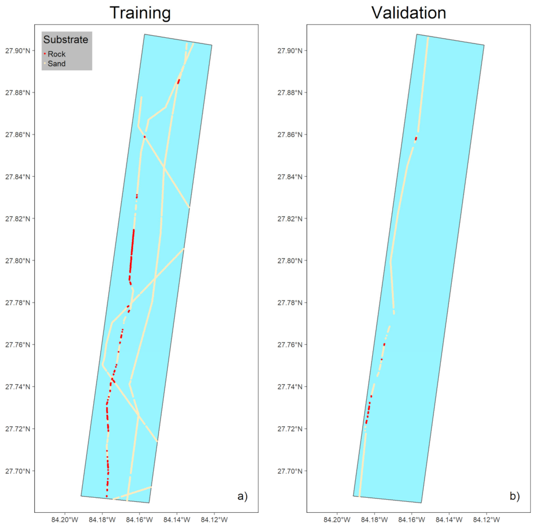
2.3.1. Response Variable: Ground-Truth Substrate Observations

Both supervised (random forest) and unsupervised (k-means clustering) statistical models were fit to predict seafloor substrate (rock vs. sand) based on the MBES data and their derivative features [10]. Ground-truth substrate classifications from the towed video were used as the response variable, and bathymetry, backscatter, and their derivative features were the predictors (independent variables) in the predictive statistical models. Due to a comparatively small number of observations for higher relief rocky habitats and their relatively small spatial size relative to the positional error associated with our towed system, these models did not attempt to predict vertical relief but rather substrate type. To reduce the influence of spatial autocorrelation on accuracy assessment, ground-truth observations from three transects were used to train the model, and one entire transect was reserved for the accuracy assessment of predictions (Figure 1). To reduce the effect of positional uncertainty of the video system and confusion due to mixed habitats or habitat boundaries [54,55,56,57], only habitat observations that were the same as their previous and subsequent observations were used to fit and assess the models.

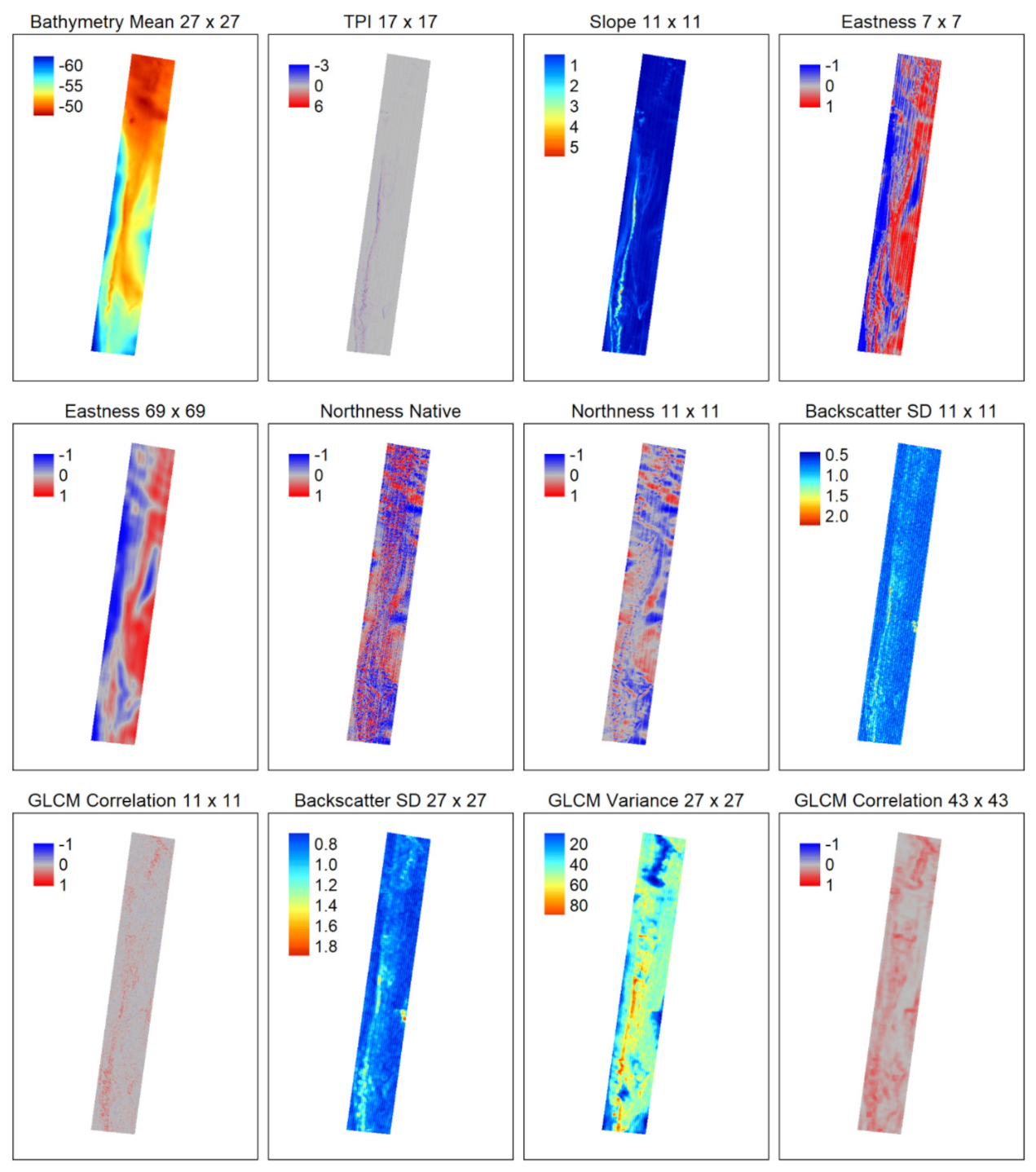
2.3.2. Predictor Variables: MBES Data and Their Derivative Features

The 10 × 10 m resolution bathymetry and backscatter grids were used to calculate various derivative metrics (

Table 1. Derivative features from the 10 m × 10 m bathymetry and backscatter surfaces for the Elbow of the west Florida shelf. Features were calculated using eight different scales of analysis from a 3 × 3 pixel to a 69 × 69 pixel moving window, and the resulting surfaces all have 10 m × 10 m resolution. Formulas for texture metrics are from Hall-Beyer [24]. N = number of rows or columns in the gray level co-occurrence matrix (GLCM) (equal to the number of gray levels, 32); i = row indices of the GLCM (equal to gray level of reference pixel); j = column indices of the GLCM (equal to gray level of neighboring pixel); P_i,j = probability (relative frequency) of neighboring pixels having gray levels i and j.

Feature	Source	Description/Algorithm
Local mean of bathymetry	Bathymetry	Mean of bathymetry in a given window
Local standard deviation of bathymetry	Bathymetry	Standard deviation of bathymetry in a given window (a measure of rugosity)
Eastness	Bathymetry	$\sin (aspect)$
Northness	Bathymetry	$\cos \left(aspect\right)$
Slope	Bathymetry	Measure of the rate of change in bathymetry
Topographic Position Index	Bathymetry	Indicates whether a location is a local high or low
Local mean of backscatter	Backscatter	Mean of backscatter in a given window
Local standard deviation of backscatter	Backscatter	Standard deviation of backscatter in a given window (a measure of heterogeneity)
GLCM Mean (µ)	Backscatter	${\displaystyle {\displaystyle \sum }_{i,j=0}^{N-1}}i\left(P_{i,j}\right)$
GLCM Variance (σ2)	Backscatter	${\displaystyle {\displaystyle \sum }_{i,j=0}^{N-1}}{P}_{i,j}{\left(1-{\mu }_i\right)}^2$
GLCM Homogeneity	Backscatter	${\displaystyle {\displaystyle \sum }_{i,j=0}^{N-1}}\frac{P_{i,j}}{1+{\left(i-j\right)}^2}$
GLCM Contrast	Backscatter	${\displaystyle {\displaystyle \sum }_{i,j=0}^{N-1}}{P}_{i,j}{(i-j)}^2$
GLCM Dissimilarity	Backscatter	${\displaystyle {\displaystyle \sum }_{i,j=0}^{N-1}}{P}_{i,j}\left|i-j\right|$
GLCM Entropy	Backscatter	${\displaystyle {\displaystyle \sum }_{i,j=0}^{N-1}}{P}_{i,j}[-\ln \left(P_{i,j}\right)]$
GLCM Angular Second Moment	Backscatter	${\displaystyle {\displaystyle \sum }_{i,j=0}^{N-1}}{P}_{i,j}^2$
GLCM Correlation	Backscatter	${\displaystyle {\displaystyle \sum }_{i,j=0}^{N-1}}{P}_{i,j}\frac{\left(i-\mu \right)\left(j-\mu \right)}{{\mathsf{\sigma }}^2}$

). These metrics include terrain attributes derived from the bathymetry surface [21,22] and texture measures derived from the backscatter mosaic using GLCMs [23,24] as well as the local mean and the standard deviation of backscatter using varying window sizes. The 10 × 10 m bathymetry and backscatter surfaces along with their derivative features were used as the predictor variables in the statistical models.

Bathymetric terrain attributes and backscatter texture metrics were computed at multiple scales of analysis by varying the window sizes over which the metrics were calculated [22]. Including predictors derived at a range of different scales is considered “best practice” in benthic habitat mapping [22,25,56,58,59]. Systematically representing multiple scales was accomplished by varying the size of the analysis window according to the Fibonacci sequence [22]. The Fibonacci sequence was used to determine the radius in number of pixels around a central pixel for eight different scales of analysis. This resulted in derivative features being calculated at eight different window sizes from 3 × 3 pixels to 69 × 69 pixels (3 × 3, 5 × 5, 7 × 7, 11 × 11, 17 × 17, 27 × 27, 43 × 43, 69 × 69; scale factors ranging from 30–690 m).

The bathymetric terrain attributes were calculated in the R programming language version 3.6.3 [60] using the raster package [61]. The terrain attributes chosen were slope, eastness and northness components of aspect (i.e., the orientation of the slope), local standard deviation of bathymetry (a measure of rugosity), local mean of bathymetry, and topographic position index (e.g., a local high or low [62]). These attributes were selected based on suggestions from Lecours et al. [21]; however, topographic position index (TPI) was substituted for relative difference from mean value (RDMV), as they both are used to determine local highs and lows, but TPI has a more intuitive meaning, and the denominator in RDMV can cause the metric to be undefined, leading to voids in the resulting surface. Horn’s method [63] was used to derive slope and aspect, as this is the most widely used and widely available algorithm for computing these metrics [21]; however, its calculation is restricted to a 3 × 3 window. To extend these metrics (slope, eastness, and northness) to multiple scales, these attributes were first derived (referred to as native scale), and then the local mean of each attribute was calculated using varying window sizes (method three in Dolan [64]).

For the backscatter derivatives, the local mean and the local standard deviation of backscatter intensity were calculated across the range of window sizes. Additionally, texture measures based on GLCMs were calculated [23,24]. Texture metrics used were GLCM contrast, GLCM dissimilarity, GLCM homogeneity, GLCM angular second momentum (ASM), GLCM entropy, GLCM mean, GLCM variance, and GLCM correlation [24]. These texture metrics can be broken down into three groups: the contrast group (contrast, dissimilarity, and homogeneity), the orderliness group (ASM and entropy), and the descriptive statistics group (mean, variance, and correlation) [24]. For the GLCM texture metrics, the 10 m x 10 m backscatter surface was first quantized to 32 gray levels (discrete integer values ranging from 0–31) using equal probability quantization [23,65]. Then, a symmetrical GLCM was tabulated in all four directions (0°/180°, 45°/225°, 90°/270°, 135°/315°, where 0° is directly to the right and degrees increase counter-clockwise), and the value of texture metrics was averaged over all directions to get directionally/rotationally invariant measures of texture. Although there are many software packages to calculate these GLCM textures, many are proprietary, and there can be inconsistencies in the results among different software [24,66]. In some cases, these inconsistencies have prevented their use in benthic habitat mapping studies [67]. For this study, free open source software was developed to calculate these texture metrics on raster data and is available as an R package [68].

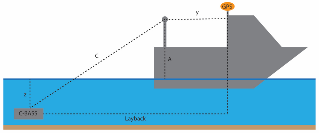
2.3.3. Estimating Towed Video Position

To associate ground-truth habitat observations from the towed video with the relevant MBES data, the position of the video at a given time must be estimated. This was done trigonometrically [15,48,69]. The layback of the of the towed video system behind the vessel was calculated using Pythagorean theorem based on the cable out from the winch, the depth of the C-BASS, the vertical offset of the height of the A-frame block relative to the waterline, and the fore/aft offset between the A-frame and the GPS antenna (Equation (1) and Figure 3). The layback was converted to a time delay by dividing it by the average speed over the preceding minute and then was used to assign C-BASS a position by assuming that the C-BASS exactly followed the ship track but lagged in time.

$$\mathrm{Layback}=\mathrm{y}+\sqrt{{\mathrm{C}}^2-{\left(\mathrm{z}+\mathrm{A}\right)}^2}$$

(1)

$\mathrm{C}: \mathrm{cable} \mathrm{out} \left(\mathrm{m}\right)$; $\mathrm{z}: \mathrm{CBASS} \mathrm{Depth} \left(\mathrm{m}\right)$; $\mathrm{A}: \mathrm{A}-\mathrm{Frame} \mathrm{height} \left(\mathrm{m}\right)$; $\mathrm{y}: \mathrm{fore}/\mathrm{aft} \mathrm{offset}$.

Figure 3. Schematic representation showing the physical meaning of the parameters from Equation (1) that were used to calculate the layback of the Camera-Based Assessment Survey System (C-BASS) system behind the ship’s GPS antenna.

Figure 3. Schematic representation showing the physical meaning of the parameters from Equation (1) that were used to calculate the layback of the Camera-Based Assessment Survey System (C-BASS) system behind the ship’s GPS antenna.

2.3.4. Classification Algorithms

Both supervised and unsupervised classification procedures were employed to predict substrate over the full area of the MBES survey [10]. The supervised classification map was created using a balanced random forest algorithm with down-sampling [70,71] via the RSToolbox [57,72] and ranger [73] R packages. The random forest algorithm has been implemented in a number of previous benthic habitat mapping studies [20,25,26,56,74,75,76] and has been found to have good performance for mapping benthic habitats when compared to other classifiers [74,77]. The random forest algorithm works much like a traditional decision tree where each node determines the optimal split in the predictor variables to best separate groups, however, rather than simply fitting one decision tree, a “forest” of many decision trees (e.g., hundreds to thousands) is fit to the data based on a bootstrap sample (sampling with replacement) of the data, and each node on a tree is only given access to a random subset of predictors [70,78]. Due to class imbalance (many more observations of sand as compared to rock), we implemented a balanced random forest algorithm using down-sampling, meaning that each bootstrap sample used to fit an individual decision tree contained an equal number of observations of each class, and the number of observations of each class was equal to the number of observations in the minority class. This has been found to be an effective way to improve predictions using unbalanced data [71]. The number of decision trees was set to 3000, and the plot of “out-of-bag” (OOB) error vs. the number of trees was used to verify that a sufficient number of trees was used by ensuring that the error rate reached an asymptote, and the number of variables available at each split was tuned to maximize Kappa using five-fold cross validation. Cohen’s Kappa (κ) is a measure of the level of agreement between two sets (often between predictions and observations). The value of Kappa is equal to one if there is complete agreement between the two sets, zero if the agreement is no greater than what could occur by chance, and negative if the agreement is less than what could occur by chance. Some rules of thumb for Kappa are that values less than zero represent poor agreement, from 0–0.2 represents slight agreement, from 0.2–0.4 represents moderate agreement, from 0.6–0.8 represents substantial agreement, and values from 0.8–1 represent almost perfect agreement [79,80].

The unsupervised statistical model used was k-means clustering [81], implemented via the RSToolbox R package [57,72]. K-means clustering is one of the most used clustering algorithms for both terrestrial and marine mapping applications [56,57] and is widely available in many different software environments. As the k-means clustering algorithm requires the number of clusters to be specified a priori, a rule of thumb is to use twice the number of the desired classes [82]. Since the desired thematic resolution was a two-class map of rock vs. sand, the k-means algorithm was run using four clusters. The ground-truth habitat points from the training data set were then used post-hoc to interpret the acoustic clusters. Each cluster was interpreted as a substrate type based on majority vote of all ground-truth habitat points from the training set contained within that cluster.

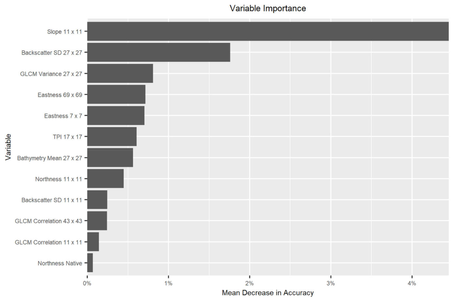
2.3.5. Variable Selection and Dimensionality Reduction

Calculating the derivative features for bathymetry and backscatter across multiple scales resulted in 130 predictor variables (Table 1). GLCM correlation was only included at five different scales (3 × 3, 5 × 5, and 7 × 7 were removed), as the metric is undefined if all values in the window have the same value, which is more likely for smaller window sizes and leads to voids in the resulting surfaces. Of these 130 predictors, many were redundant and highly correlated, thus it was necessary to conduct variable selection and dimension reduction [56].

For the supervised classification model, the Boruta selection algorithm was used to determine important predictors [77,83]. This method fits many random forest models and uses an iterative process to determine if a predictor variable has an importance score significantly greater than a permuted version of itself. The significance threshold was set at α = 0.05, and variable importance was calculated as the unscaled permutation-based mean decrease in accuracy of OOB observations [84,85]. To further reduce the number of predictors and remove high co-linearity predictors, the Pearson correlation was calculated between all remaining predictors, and a predictor was removed from the model if it was highly correlated (|r| > 0.8) with a predictor that had a higher average importance score as determined by the Boruta procedure [25,56,58]. This is similar to procedures employed in other studies (e.g., [25,58]) however, in our study, rather than including only the most important scale of a given predictor, the same predictor was allowed to be included at multiple scales based on the logic that a given predictor may be important at several different scales and may be representative of different processes, especially if those different scales are not highly correlated.

For the unsupervised classification model, all predictors (multibeam bathymetry, backscatter, and their derivative features) were z-score normalized to minimize the effects of differing ranges and units among predictors, and a principal components analysis (PCA) was conducted to remove the effect of multi-collinearity [56,86]. To remove redundant principal components (PCs), only a subset of the original PCs was retained. A PC was only retained if it explained more variance than what would be expected if the total variance was divided randomly amongst all the PCs as modeled by a broken-stick distribution [87,88,89]. The retained PCs were then used in the k-means clustering procedure [81].

2.3.6. Accuracy Assessment

Both supervised and unsupervised substrate maps were assessed using the validation transect in terms of overall, producer’s, and user’s accuracy as well as the Cohen’s Kappa statistic [90]. User’s and producer’s accuracy statistics are useful for assessing errors of omission (false negatives) and errors of commission (false positives) for each substrate type. The Kappa scores of the two maps were then compared using a Monte-Carlo permutation procedure with 999 iterations to test whether the supervised classification map had significantly greater performance (α = 0.05) than the unsupervised classification map [91].

An entropy map, which displays the uncertainty in predicted substrate for each individual pixel, was generated for the supervised classification map. Entropy was calculated based on the proportion of decision trees in the model that voted for each class within a given pixel using the Shannon entropy formula (Equation (2)) [57,92,93].

$$\mathrm{Entropy}= -{\displaystyle \sum }_{\mathrm{i}=1}^{\mathrm{M}}\left[{\mathrm{p}}_{\mathrm{i}}*\ln \left({\mathrm{p}}_{\mathrm{i}}\right)\right]$$

(2)

${\mathrm{p}}_{\mathrm{i}}: \mathrm{probability} \mathrm{that} \mathrm{a} \mathrm{cell} \mathrm{is} \mathrm{of} \mathrm{class} \mathrm{i}$; $\mathrm{i}: \mathrm{class} \mathrm{number}$; $\mathrm{M}: \mathrm{number} \mathrm{of} \mathrm{classes}$.

2.3.7. Map Comparison

To compare maps, a difference map was created to visually depict where and how classifications from each model agreed and disagreed [94]. In addition to comparing observations to predictions for accuracy assessment, Kappa can also be used to compare how well two maps agree with each other. Moreover, since, when used in the spatial context, Kappa confounds similarity in location with similarity in quantity, we can decompose Kappa into Klocation and Khisto where Kappa is the product of these two terms [80,95,96]. Klocation quantifies how well the spatial allocation of the classes agree between the two maps, and Khisto quantifies the agreement between the fraction of pixels assigned to each class [80,95,96]. As such, Kappa, Klocation, and Khisto were calculated to compare the supervised and the unsupervised classification maps.

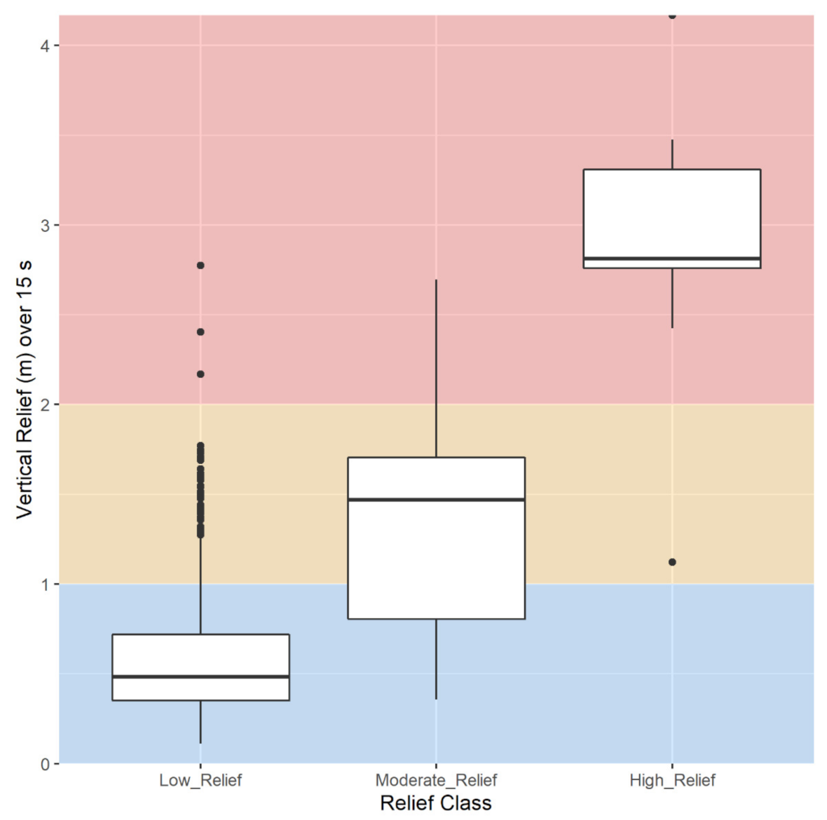
2.3.8. Vertical Relief

In addition to substrate, vertical relief was determined, as this has been found to be an important factor relating to fish community composition and abundance in many studies [34,53,97,98,99,100,101]. Vertical relief was calculated directly from the 10 m bathymetry surface using a moving 3 × 3 pixel moving window by taking the depth value of the central pixel in the window and subtracting the minimum depth of the surrounding pixels. These relief values were then reclassified into categories (low, moderate, and high relief) using the thresholds determined by Smith et al. [30] for the Florida Keys (low relief <1 m, moderate relief >1 and ≤2 m, and high relief >2 m) as these previously established thresholds corresponded well with our observations based on changes in total depth over 15 s bins as calculated from C-BASS’ onboard sensors (Figure A1). This was then layered over the best performing substrate map to delineate rock habitats of various types of relief, resulting in a final habitat map with four classes: sand, low relief rock, moderate relief rock, and high relief rock.

2.4. Fish Community Analyses and Abundance Estimates

2.4.1. Fish Densities

Using the fish counts and the corresponding habitat classifications from the video data, a species-by-site matrix of fish counts and habitat observation binned to 15 s intervals was created by associating each individual fish with the closest habitat observation in time. For each 15 s bin, fish counts were converted to densities by dividing fish counts by the cumulative area viewed in the video over the 15 s observation window (Equation (3)). The horizontal angle of view of the system in air was calculated based on the properties of the camera system [102]. This angle of view was then adjusted for the refraction of light in seawater using Snell’s Law, and the average width of the frame for each 15 s bin was calculated using the trigonometric approach of Grasty [53], which estimates the frame width using the altitude and the pitch of the camera relative to the bottom as well as the horizontal angle of view of the camera in seawater. Distance traveled by the video system was calculated using ship speed; the area viewed was calculated by multiplying the frame width by the distance traveled. For calculations, median values of the ship speed, C-BASS altitude, and C-BASS pitch over each 15 s bin were used (see Supplementary Materials for full details).

2.4.2. Multivariate Community Analysis

Differences in the fish communities among the four broad habitat types (sand, low relief rock, moderate relief rock, and high relief rock) were analyzed. If the same habitat was observed multiple times sequentially along a transect, fish counts were aggregated, and the area viewed summed across all contributing 15 s bins. Counts were converted to densities by dividing the number of fishes by the area viewed (see above for area calculations).

To assess differences in fish communities among habitats, a non-parametric permutation based analysis of variance (PERMANOVA) [103] tested the null hypothesis of no significant difference in fish community composition and abundance among habitat classes. Species composition differences among individual pairs of habitat classes were evaluated using pairwise PERMANOVA tests. Prior to conducting the PERMANOVA, the validity of the assumption of homogeneity of multivariate dispersion was checked using a multivariate analogue to the Levene’s test [104]. A canonical analysis of principal coordinates (CAP) was conducted to identify which taxa were responsible for driving these compositional differences [105]. These analyses were conducted in R using the vegan [106,107] and BiodiversityR [108,109] R packages. All fish counts were square-root-transformed to reduce the influence of occasional large aggregations, and the Bray–Curtis dissimilarity metric was used to calculate dissimilarity between samples [110]. Moreover, any observations where no fish were observed were removed for these analyses, as that is a requirement of the Bray–Curtis dissimilarity metric since it cannot be calculated based on joint species absences [110]. Significance was assessed at α = 0.05, and p-values for pair-wise comparisons were adjusted using Holm’s sequential Bonferroni procedure to account for the effect of multiple comparisons [111,112].

2.4.3. Fish Abundance Estimates

Based on the results of pairwise PERMANOVA tests, habitat classes were merged if their pairwise comparisons were not significantly different. The average density for each fish taxa by habitat type was calculated (Equation (4)) and 95% confidence intervals determined via bootstrap resampling with 999 iterations [113]. The combined map of substrate and vertical relief was used to calculate the total area of each habitat type. These areas were used to scale habitat-specific densities up to abundance estimates by multiplying the area of each habitat type by the habitat-specific density for a given taxa and then summing across habitat types to provide an estimate of total abundance for the study area (Equation (5)). The 95% confidence intervals for abundance were calculated by substituting the lower and the upper bounds of the habitat-specific density confidence intervals as ${\overline{D}}_{\mathrm{h}}$ in the calculations of abundance.

$${\mathrm{D}}_{\mathrm{b}}={\mathrm{c}}_{\mathrm{b}}/{\mathrm{A}}_{\mathrm{b}}$$

(3)

$${\overline{\mathrm{D}}}_{\mathrm{h}}= \frac{{{\displaystyle \sum }}_{\mathrm{n}=1}^{\mathrm{n}}{\mathrm{c}}_{\mathrm{b}}}{{{\displaystyle \sum }}_{\mathrm{n}=1}^{\mathrm{n}}{\mathrm{A}}_{\mathrm{b}}}=\frac{{{\displaystyle \sum }}_{\mathrm{n}=1}^{\mathrm{n}}({\mathrm{D}}_{\mathrm{b}}{*\mathrm{A}}_{\mathrm{b}})}{{{\displaystyle \sum }}_{\mathrm{n}=1}^{\mathrm{n}}{\mathrm{A}}_{\mathrm{b}}}$$

(4)

$$\mathrm{Abd}= {\displaystyle \sum }_{\mathrm{h}=1}^{\mathrm{nh}}({\overline{\mathrm{D}}}_{\mathrm{h}}{*\mathrm{A}}_{\mathrm{h}})$$

(5)

• D_b: Average density of fish taxa for bin b;
• n: number of bins for a given habitat type;
• c_b: number of fish of a given taxa in bin b;
• A_b: Aera viewed by the camera over bin b;
• ${\overline{D}}_{\mathrm{h}}$: Average density of fish taxa for habitat type b;
• Abd: Abundance of fish taxa summed across all habitat types;
• nh: number of habitat classes;
• A_h: Area of habitat type h in the entire study area.

3. Results

3.1. Predictive Habitat Mapping

3.1.1. Preparing Ground-Truth Data

The ground-truth dataset consisted of 3680 observations where each observation was the substrate classification determined from the video at 15 s intervals. This consisted of 473 observations of rock, 3195 observations of sand, and 12 observations where the substrate was not discernable. After censoring substrate determinations that differed from their previous and subsequent observations (procedure described above), those where substrate was not visible, and observations beyond the bounds of the MBES survey, there remained 238 observations of rock and 2533 observations of sand. After splitting these data into training and validation sets, the training data set consisted of 210 observations of rock and 1947 observations of sand, and the validation data consisted of 28 observations of rock and 586 observations of sand (Figure 4).

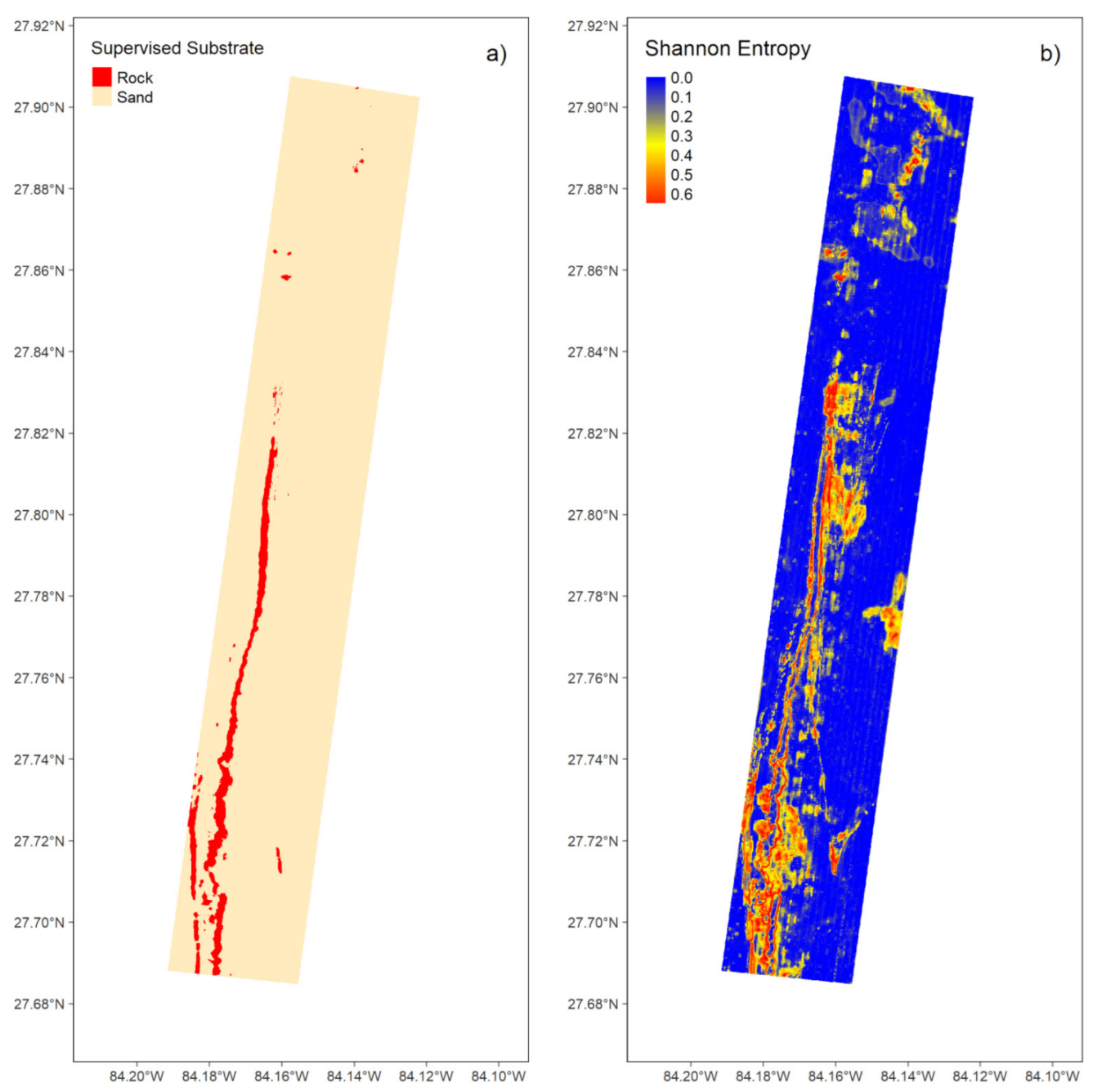
3.1.2. Supervised Classification

The Boruta variable selection procedure retained 120 of the 130 predictors; however, after removing predictors that were highly correlated with a more important predictor (|r| > 0.8), only 12 predictor variables remained. These predictors were local mean of bathymetry (27 × 27), TPI (17 × 17), slope (11 × 11), eastness (7 × 7 and 69 × 69), northness (native and 11 × 11), local standard deviation of backscatter (11 × 11 and 27 × 27), GLCM correlation (11 × 11 and 43 × 43), and GLCM variance (27 × 27; Figure 5). After variable selection, the optimal number of variables available at each split was determined to be four, and the number of decision trees was found to be sufficient (Figure A2). The tuned and fitted model was then used to predict substrate for the entire study area, resulting in a map consisting of 3.82 km² of rock and 83.75 km² of sand (Figure 6). Accuracy assessment was performed on the validation data; the confusion matrix with performance metrics is presented in

Table 2. Confusion matrix and user’s (row-wise) accuracy, producer’s (column-wise) accuracy, overall accuracy, and Cohen’s Kappa statistic (κ) for the substrate map of the Elbow of the west Florida shelf derived using supervised classification.

	Rock	Sand	User’s Accuracy
Rock	23	9	71.9%
Sand	5	575	99.1%
Producer’s Accuracy	82.1%	98.5%	Overall Accuracy	97.7%
			κ	0.75

.

The variable importance is shown in Figure 7. The most important predictor was slope (11 × 11), followed by standard deviation of backscatter (27 × 27). Although some predictors were more important than others, all predictors had positive values indicating that they all provided some benefit to the model’s overall predictive ability (Figure 7). Uncertainty in predicted substrate for each individual pixel is presented in the entropy map (Figure 6b).

3.1.3. Unsupervised Classification

The first nine PCs explained more variance than could be expected if the total variance was divided randomly amongst the PCs (Figure 8), and as such, they were retained for use in k-means clustering (Figure 9). The nine PCs explained 86% of the total variance. A k-means clustering procedure with four clusters was conducted on the retained PC layers (Figure 10a). Acoustically derived clusters were then assigned to substrate classes based on the majority of the ground-truth points within that cluster (

Table 3. Substrate interpretation of the map of the four acoustic clusters of the Elbow determined through k-means clustering (Figure 10a) using the ground-truth habitat observations from towed video in the training set (Figure 4a). The number of ground-truth points of each substrate type within an acoustic cluster were counted, and the acoustic cluster was assigned a substrate type based on the class of the majority of the images contained within that acoustic cluster.

Cluster	Rock Observations	Sand Observations	Assigned Substrate
1	21	229	Sand
2	179	75	Rock
3	10	1447	Sand
4	0	194	Sand

and Figure 10b). This substrate map predicts the study area to consist of 3.74 km² of rock and 83.83 km² of sand. Accuracy assessment was performed on the validation data; the confusion matrix with performance metrics is presented in

Table 4. Confusion matrix and user’s (row-wise) accuracy, producer’s (column-wise) accuracy, overall accuracy, and Cohen’s Kappa statistic (κ) for the substrate map of the Elbow of the west Florida shelf derived using unsupervised classification.

	Rock	Sand	User’s Accuracy
Rock	10	0	100.0%
Sand	18	585	97.0%
Producer’s Accuracy	35.7%	100.0%	Overall Accuracy	97.1%
			κ	0.51

.

3.1.4. Map Comparison

The supervised substrate map predicted 0.08 km² more rock than the unsupervised substrate map. These differences can be visualized in Figure 11. The two maps agree 98.33% of the time; the supervised classification map predicts rock where the unsupervised classification map predicts sand 0.87% of the time, and the supervised map predicts sand where the unsupervised map predicts rock 0.80% of the time. The comparison of Kappa, Klocation, and Khisto shows “almost perfect agreement” in both the spatial allocation and the relative frequency of class assignment (Klocation = 0.807 and Khisto of 0.989). Overall, this corresponds to a Kappa value (Klocation*Khisto) of 0.798, indicating a “substantial level” of agreement between the two maps. When comparing the predictions on the validation data set for accuracy assessment, the supervised classification model was found to have greater performance (κ = 0.75 vs. κ = 0.51). This difference was found to be significant (p = 0.001) using a one-tailed Monte-Carlo permutation test, indicating that the supervised classification procedure had significantly greater predictive performance than did the unsupervised classification method.

3.1.5. Vertical Relief

The reclassified relief map was layered onto the substrate map created using the supervised classification procedure, as it had better performance than the unsupervised procedure, to create a “habitat map” consisting of a combination of substrate and vertical relief (Figure 12). This map predicts 83.75 km² of sand, 3.46 km² low relief rock, 0.31 km² of moderate relief rock, and 0.05 km² of high relief rock.

3.2. Fish Community Analyses and Abundance Estimates

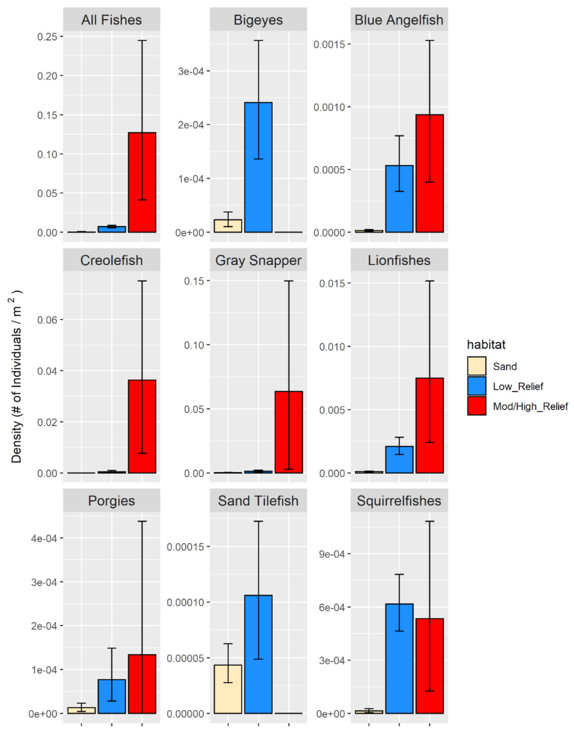
3.2.1. Fish Densities

The average densities for each fish taxon by habitat type were calculated; however, moderate and high relief rock were merged into one category since the fish communities in them were not found to be significantly different in the pairwise comparisons (see next section). Fish densities were estimated by habitat type for 36 species or species groups as well as for all fishes combined. For most taxa (33 of the 36 species/species groups), average fish density was highest over rocky habitats, and only three species (Rainbow Runner, remora spp., and Pearly Razorfish) had their highest densities over sand. Of the 33 taxa with highest densities over rocky habitat, 17 had highest densities over moderate to high relief rock and 16 over low relief rock (Figure 13 and

Table A1. Habitat-specific densities for all observed taxa in number of individuals/m² as determined from the towed video transects in the Elbow area of the west Florida shelf. Lower and upper bounds represent the 95% confidence intervals.

Taxa	Habitat	Lower Bound	Mean	Upper Bound
All_Fish	Sand	0.000305091368	0.000464386728	0.000675358543
All_Fish	Low_Relief	0.005654144932	0.007306868473	0.008924795926
All_Fish	Mod/High_Relief	0.041204024881	0.127203256069	0.245024232512
amberjack_spp	Sand	0.000000000000	0.000002902417	0.000007282130
amberjack_spp	Low_Relief	0.000038238047	0.000404866063	0.000988826791
amberjack_spp	Mod/High_Relief	0.000000000000	0.000133616866	0.000390694044
angelfish_blue	Sand	0.000005804730	0.000014512085	0.000023436164
angelfish_blue	Low_Relief	0.000326755837	0.000530181749	0.000767483569
angelfish_blue	Mod/High_Relief	0.000399268295	0.000935318059	0.001528539056
angelfish_gray	Sand	0.000000000000	0.000000000000	0.000000000000
angelfish_gray	Low_Relief	0.000009508321	0.000057838009	0.000126721804
angelfish_gray	Mod/High_Relief	0.000000000000	0.000133616866	0.000426533497
angelfish_spp	Sand	0.000000000000	0.000000000000	0.000000000000
angelfish_spp	Low_Relief	0.000000000000	0.000009639668	0.000029689030
angelfish_spp	Mod/High_Relief	0.000000000000	0.000000000000	0.000000000000
bigeye_spp	Sand	0.000010242236	0.000023219336	0.000037805805
bigeye_spp	Low_Relief	0.000136342357	0.000240991704	0.000356470592
bigeye_spp	Mod/High_Relief	0.000000000000	0.000000000000	0.000000000000
boxfish_spp	Sand	0.000000000000	0.000000000000	0.000000000000
boxfish_spp	Low_Relief	0.000000000000	0.000019279336	0.000048421997
boxfish_spp	Mod/High_Relief	0.000000000000	0.000000000000	0.000000000000
butterflyfish_spp	Sand	0.000000000000	0.000002902417	0.000007276943
butterflyfish_spp	Low_Relief	0.000009548271	0.000048198341	0.000105886188
butterflyfish_spp	Mod/High_Relief	0.000000000000	0.000000000000	0.000000000000
eel_spp	Sand	0.000000000000	0.000000000000	0.000000000000
eel_spp	Low_Relief	0.000000000000	0.000009639668	0.000029404678
eel_spp	Mod/High_Relief	0.000000000000	0.000000000000	0.000000000000
goatfish_spotted	Sand	0.000000000000	0.000000000000	0.000000000000
goatfish_spotted	Low_Relief	0.000000000000	0.000000000000	0.000000000000
goatfish_spotted	Mod/High_Relief	0.000000000000	0.000133616866	0.000430797429
grouper_black	Sand	0.000000000000	0.000000000000	0.000000000000
grouper_black	Low_Relief	0.000000000000	0.000000000000	0.000000000000
grouper_black	Mod/High_Relief	0.000000000000	0.000400850597	0.001324759414
grouper_creolefish	Sand	0.000000000000	0.000000000000	0.000000000000
grouper_creolefish	Low_Relief	0.000000000000	0.000356667722	0.000928362228
grouper_creolefish	Mod/High_Relief	0.007643028251	0.036343787448	0.075195350579
grouper_gag	Sand	0.000000000000	0.000001451209	0.000004381866
grouper_gag	Low_Relief	0.000000000000	0.000019279336	0.000059046688
grouper_gag	Mod/High_Relief	0.000000000000	0.000267233731	0.000852786071
grouper_goliath	Sand	0.000000000000	0.000000000000	0.000000000000
grouper_goliath	Low_Relief	0.000000000000	0.000000000000	0.000000000000
grouper_goliath	Mod/High_Relief	0.000000000000	0.000400850597	0.001065084821
grouper_red	Sand	0.000000000000	0.000001451209	0.000004381866
grouper_red	Low_Relief	0.000009425807	0.000038558673	0.000078463175
grouper_red	Mod/High_Relief	0.000000000000	0.000000000000	0.000000000000
grouper_scamp	Sand	0.000000000000	0.000000000000	0.000000000000
grouper_scamp	Low_Relief	0.000009680947	0.000144595023	0.000359476725
grouper_scamp	Mod/High_Relief	0.000000000000	0.000133616866	0.000430797429
grouper_spp	Sand	0.000001443556	0.000005804834	0.000011675402
grouper_spp	Low_Relief	0.000000000000	0.000019279336	0.000048726459
grouper_spp	Mod/High_Relief	0.000000000000	0.000133616866	0.000426393036
jack_crevalle	Sand	0.000000000000	0.000001451209	0.000004375663
jack_crevalle	Low_Relief	0.000000000000	0.000028919005	0.000077360701
jack_crevalle	Mod/High_Relief	0.000000000000	0.000000000000	0.000000000000
jack_rainbowrunner	Sand	0.000000000000	0.000002902417	0.000008756979
jack_rainbowrunner	Low_Relief	0.000000000000	0.000000000000	0.000000000000
jack_rainbowrunner	Mod/High_Relief	0.000000000000	0.000000000000	0.000000000000
jack_spp	Sand	0.000000000000	0.000000000000	0.000000000000
jack_spp	Low_Relief	0.000000000000	0.000009639668	0.000029677705
jack_spp	Mod/High_Relief	0.000000000000	0.000000000000	0.000000000000
lionfish_spp	Sand	0.000056869715	0.000094328554	0.000134798264
lionfish_spp	Low_Relief	0.001457130610	0.002091807993	0.002804478909
lionfish_spp	Mod/High_Relief	0.002402247287	0.007482544475	0.015170870783
porgy_spp	Sand	0.000004360488	0.000013060877	0.000023075921
porgy_spp	Low_Relief	0.000028376948	0.000077117345	0.000148411135
porgy_spp	Mod/High_Relief	0.000000000000	0.000133616866	0.000437293986
remora_spp	Sand	0.000000000000	0.000001451209	0.000004377825
remora_spp	Low_Relief	0.000000000000	0.000000000000	0.000000000000
remora_spp	Mod/High_Relief	0.000000000000	0.000000000000	0.000000000000
shark_spp	Sand	0.000000000000	0.000000000000	0.000000000000
shark_spp	Low_Relief	0.000000000000	0.000009639668	0.000029219565
shark_spp	Mod/High_Relief	0.000000000000	0.000000000000	0.000000000000
snapper_gray	Sand	0.000013061514	0.000108840639	0.000254981252
snapper_gray	Low_Relief	0.000468269192	0.001156760180	0.002055718899
snapper_gray	Mod/High_Relief	0.002742580078	0.063468011169	0.149759809054
snapper_spp	Sand	0.000000000000	0.000000000000	0.000000000000
snapper_spp	Low_Relief	0.000000000000	0.000019279336	0.000059229663
snapper_spp	Mod/High_Relief	0.000000000000	0.000133616866	0.000390694044
snapper_yellowtail	Sand	0.000000000000	0.000000000000	0.000000000000
snapper_yellowtail	Low_Relief	0.000000000000	0.000038558673	0.000116011333
snapper_yellowtail	Mod/High_Relief	0.000000000000	0.000267233731	0.000809175808
squirrelfish_spp	Sand	0.000004354164	0.000014512085	0.000026267894
squirrelfish_spp	Low_Relief	0.000464723937	0.000616938763	0.000782913741
squirrelfish_spp	Mod/High_Relief	0.000125668348	0.000534467462	0.001081371358
stingray_spp	Sand	0.000000000000	0.000000000000	0.000000000000
stingray_spp	Low_Relief	0.000000000000	0.000009639668	0.000029666787
stingray_spp	Mod/High_Relief	0.000000000000	0.000000000000	0.000000000000
surgeonfish_spp	Sand	0.000000000000	0.000001451209	0.000004388087
surgeonfish_spp	Low_Relief	0.000057776382	0.000134955354	0.000233778550
surgeonfish_spp	Mod/High_Relief	0.000000000000	0.000000000000	0.000000000000
tilefish_sand	Sand	0.000027559370	0.000043536256	0.000062686638
tilefish_sand	Low_Relief	0.000048742988	0.000106036350	0.000172505726
tilefish_sand	Mod/High_Relief	0.000000000000	0.000000000000	0.000000000000
triggerfish_spp	Sand	0.000000000000	0.000004353626	0.000010194629
triggerfish_spp	Low_Relief	0.000009284980	0.000038558673	0.000078463175
triggerfish_spp	Mod/High_Relief	0.000000000000	0.000000000000	0.000000000000
wrasse_creole	Sand	0.000000000000	0.000000000000	0.000000000000
wrasse_creole	Low_Relief	0.000000000000	0.000000000000	0.000000000000
wrasse_creole	Mod/High_Relief	0.000000000000	0.001336168656	0.004307974287
wrasse_hogfish	Sand	0.000000000000	0.000001451209	0.000004377401
wrasse_hogfish	Low_Relief	0.000009404868	0.000038558673	0.000078650541
wrasse_hogfish	Mod/High_Relief	0.000000000000	0.000133616866	0.000418370109
wrasse_pearlyrazorfish	Sand	0.000000000000	0.000001451209	0.000004378067
wrasse_pearlyrazorfish	Low_Relief	0.000000000000	0.000000000000	0.000000000000
wrasse_pearlyrazorfish	Mod/High_Relief	0.000000000000	0.000000000000	0.000000000000
wrasse_spanishhogfish	Sand	0.000000000000	0.000000000000	0.000000000000
wrasse_spanishhogfish	Low_Relief	0.000000000000	0.000000000000	0.000000000000
wrasse_spanishhogfish	Mod/High_Relief	0.000000000000	0.000267233731	0.000654899428
wrasse_spotfinhogfish	Sand	0.000000000000	0.000000000000	0.000000000000
wrasse_spotfinhogfish	Low_Relief	0.000000000000	0.000009639668	0.000029467959
wrasse_spotfinhogfish	Mod/High_Relief	0.000000000000	0.000133616866	0.000421591353

).

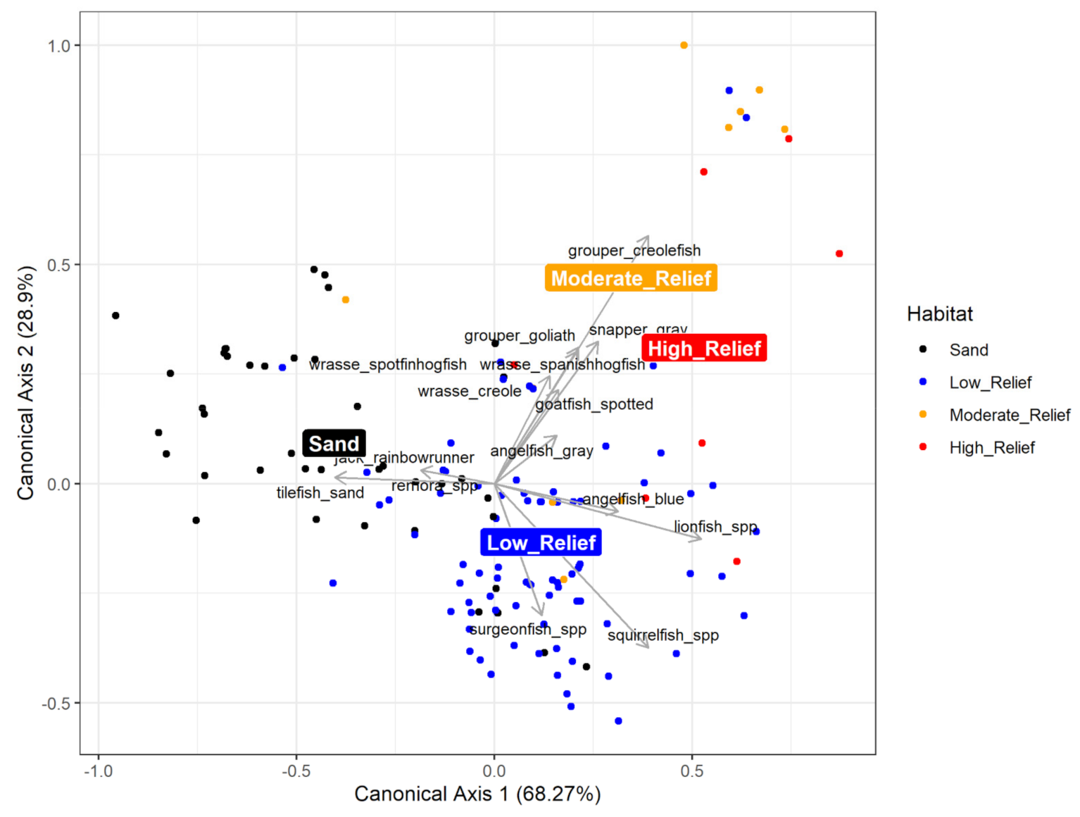
3.2.2. Multivariate Community Analysis

A total of 2030 different individual fish were observed, spanning at least 32 different species and 18 different families (

Table A2. List of all fish taxa observed along with the number of individuals seen.

Common Name	Scientific Name	Family	Order	Number of Individuals Observed
Amberjack spp.	Seriola spp.	Carangidae	Perciformes	45
		(Jacks)
Angelfish spp.		Pomacanthidae	Perciformes	1
		(Angelfishes)
Blue Angelfish	Holacanthus bermudensis	Pomacanthidae	Perciformes	72
		(Angelfishes)
Gray Angelfish	Pomacanthus arcuatus	Pomacanthidae	Perciformes	7
		(Angelfishes)
Bigeye spp.		Priacanthidae	Perciformes	41
		(Bigeyes)
Boxfish spp.		Ostraciidae	Tetraodontiformes	2
		(Boxfishes)
Butterflyfish spp.		Chaetodontidae	Perciformes	7
		(Butterflyfishes)
Eel spp.			Anguilliformes	1
Spotted Goatfish	Pseudupeneus maculatus	Mullidae	Perciformes	1
		(Goatfishes)
Grouper spp.		Serranidae	Perciformes	7
		(Groupers and Sea Basses)
Black Grouper	Mycteroperca bonaci	Serranidae	Perciformes	3
		(Groupers and Sea Basses)
Atlantic Creolefish	Paranthias furcifer	Serranidae	Perciformes	309
		(Groupers and Sea Basses)
Gag Grouper	Mycteroperca microlepis	Serranidae	Perciformes	5
		(Groupers and Sea Basses)
Goliath Grouper	Epinephelus itajara	Serranidae	Perciformes	3
		(Groupers and Sea Basses)
Red Grouper	Epinephelus morio	Serranidae	Perciformes	5
		(Groupers and Sea Basses)
Scamp	Mycteroperca phenax	Serranidae	Perciformes	16
		(Groupers and Sea Basses)
Jack spp.		Carangidae	Perciformes	1
		(Jacks)
Crevalle Jack	Caranx hippos	Carangidae	Perciformes	4
		(Jacks)
Rainbow Runner	Elagatis bipinnulata	Carangidae	Perciformes	2
		(Jacks)
Lionfish spp.	Pterois spp.	Scorpaenidae	Scorpaeniformes	338
		(Scorpionfishes)
Porgy spp.		Sparidae	Perciformes	18
		(Porgies)
Remora spp.		Echeneidae	Perciformes	1
		(Remoras)
Shark spp.			Superorder: Selachimorpha	1
Snapper spp.		Lutjanidae	Perciformes	3
		(Snappers)
Gray Snapper	Lutjanus griseus	Lutjanidae	Perciformes	670
		(Snappers)
Yellowtail Snapper	Ocyurus chrysurus	Lutjanidae	Perciformes	6
		(Snappers)
Squirrelfish spp.		Holocentridae	Beryciformes	78
		(squirrelfishes)
Whiptail stingray spp.		Dasyatidae	Rajiformes	1
		(Whiptail Stingrays)
Surgeonfish spp.		Acanthuridae	Perciformes	15
		(Surgeonfishes)
Sand Tilefish	Malacanthus plumieri	Malacanthidae	Perciformes	41
		(tilefishes)
Triggerfish spp.		Balistidae	Tetraodontiformes	7
		(Triggerfishes)
Creole Wrasse	Clepticus parrae	Labridae	Perciformes	10
		(Wrasses)
Hogfish	Lachnolaimus maximus	Labridae	Perciformes	6
		(Wrasses)
Pearly Razorfish	Xyrichtys novacula	Labridae	Perciformes	1
		(Wrasses)
Spanish Hogfish	Bodianus rufus	Labridae	Perciformes	2
		(Wrasses)
Spotfin Hogfish	Bodianus pulchellus	Labridae	Perciformes	2
		(Wrasses)
Large No ID				298

) along the three observed video transects. After combining sequential 15 s bins of the same habitat into one observation and removing observations where no fish were present, there were 41 observations over sand, 80 over low relief rock, 10 over moderate relief rock, and 7 over high relief rock. The dispersions among different habitats were found not to be significantly different (p = 0.186), indicating that the assumption of homogeneity of multivariate dispersion was met. The PERMANOVA showed that the fish community compositions differed significantly among habitat types (

Table 5. Results of the PERMANOVA assessing the null hypothesis of no significant difference in fish communities among the four habitat types: sand, low relief rock, moderate relief rock, and high relief rock.

	Degrees of Freedom	Sum of Squares	Mean Square	F	p
Habitat	3	4.762	1.58737	4.4454	0.001
Residual	134	47.849	0.35708
Total	137	52.611

, p = 0.001), and the pairwise comparisons found that all habitat types significantly differed from one another except between moderate and high relief rock (

Table 6. Results of the pairwise PERMANOVA tests with 9999 iterations to assess differences in fish communities between each pair of habitat types. The F statistic, a p value, and an adjusted p value using a sequential Bonferroni procedure to account for multiple comparisons are reported.

Comparison	F	p	Adjusted p
Sand vs. Low Relief Rock	8.685	0.0001	0.0006
Sand vs. Moderate Relief Rock	3.114	0.0006	0.0024
Sand vs. High Relief Rock	3.513	0.0002	0.0010
Low Relief Rock vs. Moderate Relief Rock	2.727	0.0066	0.0198
Low Relief Rock vs. High Relief Rock	2.410	0.0165	0.0330
Moderate Relief Rock vs. High Relief Rock	0.839	0.5773	0.5773

).

The CAP results indicated that communities over moderate and high relief rock were differentiated by having more Creolefish, Gray Snapper, Goliath Grouper, and Spanish Hogfish; low relief rocky habitats were differentiated by squirrelfishes, Blue Angelfish, lionfishes, and surgeon fishes; sand communities were differentiated by Sand Tilefish, Rainbow Runner, and remoras (Figure 14).

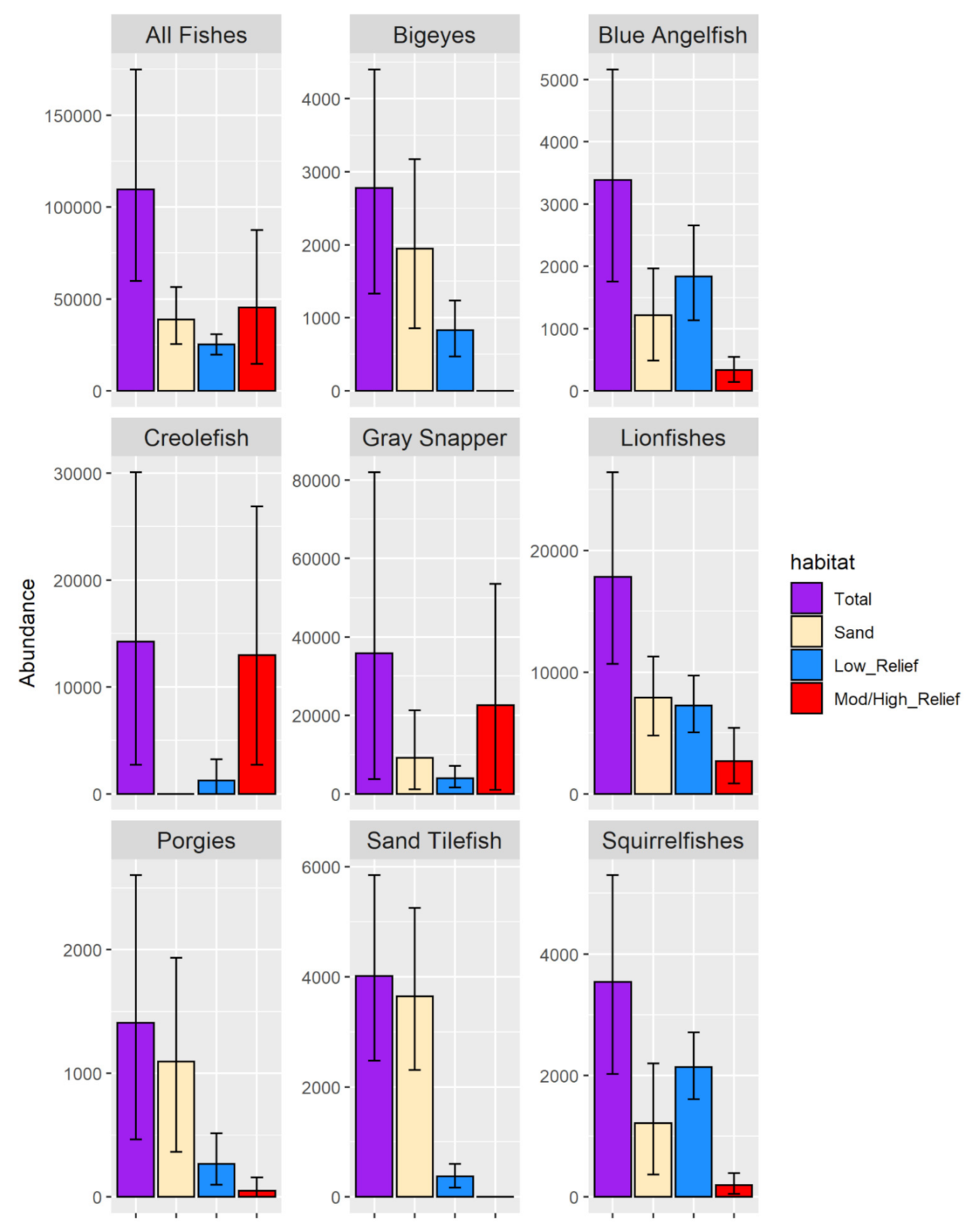
3.2.3. Fish Abundance Estimates

We estimated 110,000 fish (95% CI (59842, 174961)) ≥15 cm in length within the 88 km² study area (Figure 15 and

Table A3. Estimates of total abundance for all observed taxa within the portion of Elbow on the west Florida shelf that was mapped using a MBES. The calculated contributions of each habitat type (sand, low relief rock, and moderate to high relief rock) to the estimated total abundance are also shown. Extrapolations are based on the habitat-specific densities (Table A1 and Figure 13), and the area of each habitat based on the combined substrate and relief map (Figure 12). Upper and lower bounds represent the 95% bootstrap confidence intervals.

Taxa	Habitat	Lower Bound	Mean	Upper Bound
All_Fish	Total	59,842	109,616	174,961
All_Fish	Sand	25,552	38,893	56,563
All_Fish	Low_Relief	19,576	25,299	30,900
All_Fish	Mod/High_Relief	14,714	45,424	87,498
amberjack_spp	Total	132	1693	4173
amberjack_spp	Sand	0	243	610
amberjack_spp	Low_Relief	132	1402	3424
amberjack_spp	Mod/High_Relief	0	48	140
angelfish_blue	Total	1760	3385	5166
angelfish_blue	Sand	486	1215	1963
angelfish_blue	Low_Relief	1131	1836	2657
angelfish_blue	Mod/High_Relief	143	334	546
angelfish_gray	Total	33	248	591
angelfish_gray	Sand	0	0	0
angelfish_gray	Low_Relief	33	200	439
angelfish_gray	Mod/High_Relief	0	48	152
angelfish_spp	Total	0	33	103
angelfish_spp	Sand	0	0	0
angelfish_spp	Low_Relief	0	33	103
angelfish_spp	Mod/High_Relief	0	0	0
bigeye_spp	Total	1330	2779	4401
bigeye_spp	Sand	858	1945	3166
bigeye_spp	Low_Relief	472	834	1234
bigeye_spp	Mod/High_Relief	0	0	0
boxfish_spp	Total	0	67	168
boxfish_spp	Sand	0	0	0
boxfish_spp	Low_Relief	0	67	168
boxfish_spp	Mod/High_Relief	0	0	0
butterflyfish_spp	Total	33	410	976
butterflyfish_spp	Sand	0	243	609
butterflyfish_spp	Low_Relief	33	167	367
butterflyfish_spp	Mod/High_Relief	0	0	0
eel_spp	Total	0	33	102
eel_spp	Sand	0	0	0
eel_spp	Low_Relief	0	33	102
eel_spp	Mod/High_Relief	0	0	0
goatfish_spotted	Total	0	48	154
goatfish_spotted	Sand	0	0	0
goatfish_spotted	Low_Relief	0	0	0
goatfish_spotted	Mod/High_Relief	0	48	154
grouper_black	Total	0	143	473
grouper_black	Sand	0	0	0
grouper_black	Low_Relief	0	0	0
grouper_black	Mod/High_Relief	0	143	473
grouper_creolefish	Total	2729	14,213	30,067
grouper_creolefish	Sand	0	0	0
grouper_creolefish	Low_Relief	0	1235	3214
grouper_creolefish	Mod/High_Relief	2729	12,978	26,852
grouper_gag	Total	0	284	876
grouper_gag	Sand	0	122	367
grouper_gag	Low_Relief	0	67	204
grouper_gag	Mod/High_Relief	0	95	305
grouper_goliath	Total	0	143	380
grouper_goliath	Sand	0	0	0
grouper_goliath	Low_Relief	0	0	0
grouper_goliath	Mod/High_Relief	0	143	380
grouper_red	Total	33	255	639
grouper_red	Sand	0	122	367
grouper_red	Low_Relief	33	134	272
grouper_red	Mod/High_Relief	0	0	0
grouper_scamp	Total	34	548	1398
grouper_scamp	Sand	0	0	0
grouper_scamp	Low_Relief	34	501	1245
grouper_scamp	Mod/High_Relief	0	48	154
grouper_spp	Total	121	601	1299
grouper_spp	Sand	121	486	978
grouper_spp	Low_Relief	0	67	169
grouper_spp	Mod/High_Relief	0	48	152
jack_crevalle	Total	0	222	634
jack_crevalle	Sand	0	122	366
jack_crevalle	Low_Relief	0	100	268
jack_crevalle	Mod/High_Relief	0	0	0
jack_rainbowrunner	Total	0	243	733
jack_rainbowrunner	Sand	0	243	733
jack_rainbowrunner	Low_Relief	0	0	0
jack_rainbowrunner	Mod/High_Relief	0	0	0
jack_spp	Total	0	33	103
jack_spp	Sand	0	0	0
jack_spp	Low_Relief	0	33	103
jack_spp	Mod/High_Relief	0	0	0
lionfish_spp	Total	10,666	17,815	26,417
lionfish_spp	Sand	4763	7900	11,290
lionfish_spp	Low_Relief	5045	7242	9710
lionfish_spp	Mod/High_Relief	858	2672	5418
porgy_spp	Total	463	1409	2603
porgy_spp	Sand	365	1094	1933
porgy_spp	Low_Relief	98	267	514
porgy_spp	Mod/High_Relief	0	48	156
remora_spp	Total	0	122	367
remora_spp	Sand	0	122	367
remora_spp	Low_Relief	0	0	0
remora_spp	Mod/High_Relief	0	0	0
shark_spp	Total	0	33	101
shark_spp	Sand	0	0	0
shark_spp	Low_Relief	0	33	101
shark_spp	Mod/High_Relief	0	0	0
snapper_gray	Total	3695	35,785	81,952
snapper_gray	Sand	1094	9116	21,355
snapper_gray	Low_Relief	1621	4005	7118
snapper_gray	Mod/High_Relief	979	22,664	53,479
snapper_spp	Total	0	114	345
snapper_spp	Sand	0	0	0
snapper_spp	Low_Relief	0	67	205
snapper_spp	Mod/High_Relief	0	48	140
snapper_yellowtail	Total	0	229	691
snapper_yellowtail	Sand	0	0	0
snapper_yellowtail	Low_Relief	0	134	402
snapper_yellowtail	Mod/High_Relief	0	95	289
squirrelfish_spp	Total	2019	3542	5297
squirrelfish_spp	Sand	365	1215	2200
squirrelfish_spp	Low_Relief	1609	2136	2711
squirrelfish_spp	Mod/High_Relief	45	191	386
stingray_spp	Total	0	33	103
stingray_spp	Sand	0	0	0
stingray_spp	Low_Relief	0	33	103
stingray_spp	Mod/High_Relief	0	0	0
surgeonfish_spp	Total	200	589	1177
surgeonfish_spp	Sand	0	122	368
surgeonfish_spp	Low_Relief	200	467	809
surgeonfish_spp	Mod/High_Relief	0	0	0
tilefish_sand	Total	2477	4013	5847
tilefish_sand	Sand	2308	3646	5250
tilefish_sand	Low_Relief	169	367	597
tilefish_sand	Mod/High_Relief	0	0	0
triggerfish_spp	Total	32	498	1125
triggerfish_spp	Sand	0	365	854
triggerfish_spp	Low_Relief	32	134	272
triggerfish_spp	Mod/High_Relief	0	0	0
wrasse_creole	Total	0	477	1538
wrasse_creole	Sand	0	0	0
wrasse_creole	Low_Relief	0	0	0
wrasse_creole	Mod/High_Relief	0	477	1538
wrasse_hogfish	Total	33	303	788
wrasse_hogfish	Sand	0	122	367
wrasse_hogfish	Low_Relief	33	134	272
wrasse_hogfish	Mod/High_Relief	0	48	149
wrasse_pearlyrazorfish	Total	0	122	367
wrasse_pearlyrazorfish	Sand	0	122	367
wrasse_pearlyrazorfish	Low_Relief	0	0	0
wrasse_pearlyrazorfish	Mod/High_Relief	0	0	0
wrasse_spanishhogfish	Total	0	95	234
wrasse_spanishhogfish	Sand	0	0	0
wrasse_spanishhogfish	Low_Relief	0	0	0
wrasse_spanishhogfish	Mod/High_Relief	0	95	234
wrasse_spotfinhogfish	Total	0	81	253
wrasse_spotfinhogfish	Sand	0	0	0
wrasse_spotfinhogfish	Low_Relief	0	33	102
wrasse_spotfinhogfish	Mod/High_Relief	0	48	151

). Of these, 39,000 (35%) were predicted to be over sand, 25,000 (23%) over low relief rock, and 45,000 (41%) over moderate to high relief rock (Figure 15).

4. Discussion

4.1. Comparison of the Supervised and Unsupervised Procedures

Both the supervised and the unsupervised map classification procedures resulted in maps of the study area with the same general configurations; both maps identified the main long rocky ridge running north to south, a smaller ridge to the west, and several small rocky outcroppings (Figure 6a and Figure 10b). The maps looked very similar based on a visual inspection, and this was verified statistically as the maps exhibited “substantial agreement” overall and “almost perfect agreement” in terms of both spatial allocation and relative frequency of class assignment. Inspection of the difference map showed that the disagreement was mainly in transitional areas at the boundary of features. Additionally, both the supervised and the unsupervised substrate maps had very high accuracy (>97%) when predicting the validation data. However, overall accuracy can be a misleading metric when classes are highly unbalanced [90,114]. Accordingly, it is critical to evaluate maps using both user’s and producer’s accuracy as well as the Kappa statistic, which accounts for agreement that could occur by chance [90]. Both maps had high user’s and producer’s accuracies for sand. However, for rock (the rarer class), the unsupervised classification showed a moderately higher user’s accuracy than did the supervised map (100% vs. 71.9%) but had a much lower producer’s accuracy (35.7% vs. 82.1%). Thus, the unsupervised classification only predicted rock if it was very certain, leading to high errors of omission (false negatives). This in turn meant that the unsupervised classification was likely underpredicting the area of rock habitats, which is consistent with the finding that the supervised classification map predicted slightly more rock than the unsupervised classification map (an additional 0.08 km²). Additionally, in the difference map, it was more common to see instances where the supervised classification map predicted rock and the unsupervised map predicted sand as opposed to vice versa (Figure 11), especially in areas further from the training data. This, along with the supervised model’s greater performance on the validation data, indicated that the supervised model was more generalizable than the unsupervised model for predictions on new data. There are tradeoffs between overall accuracy and user’s and producer’s accuracy for each class. Examination of the Kappa statistic, however, indicated the supervised methodology performed better than the unsupervised methodology, and a Monte-Carlo procedure determined this difference to be significant (p = 0.001). In the supervised classification map, κ > 0.6, indicating “substantial agreement” between predictions and observations, while in the unsupervised classification map, κ > 0.4, indicating “moderate agreement” between predictions and observations. Although the supervised classification map performed better, the unsupervised procedure can still be useful. Particularly, the determination of acoustic clusters (Figure 10a) can be very valuable for designing the initial ground-truthing surveys, as one can make sure to sample within each acoustic cluster to maximize the likelihood that the full diversity of habitats in the area is sampled.

In addition to accuracy assessment, for the supervised methodology, we mapped the uncertainty in the classification for each individual pixel (Figure 6b). This gave us a picture of how uncertainty changed throughout the study area rather than just the average. Generally, the most uncertainty was found in rocky areas. However, some other areas also had moderate uncertainty. These other areas may represent differing morphologies of rock and sand habitats other than the ones from which the model was trained—mixed habitat classes, areas with gravel or debris, or entirely new habitats that were not observed in the video transects. This makes sense, as rock is the rarer substrate class, thus there are fewer samples upon which to train the model, and high complexity areas and habitat boundaries tend to have greater errors [56,115,116]. To improve the uncertainty within these areas, additional ground-truthing efforts would be needed to collect more observations in these areas. Assessing the uncertainty in a spatial context is very important, as the accuracy statistics calculated from the confusion matrix simply describe “average” uncertainty, but uncertainty is variable across the study area (Figure 6b) [56,117]. Despite being important, uncertainty in spatial classification of habitats is rarely assessed in benthic habitat mapping studies [56]. The entropy map presented herein provides a method to visually depict uncertainty regardless of the number of habitat classes and can be used with other classifiers as long as the model used is capable of outputting class probabilities [57,92,93]. Additionally, another simple way to represent the (un)certainty over space is to map the probabilities of the assigned class at each pixel location or, conversely, one minus that to display the uncertainty in the classification.

4.2. Variable Importance for Substrate Mapping

Of the many predictor variables considered, most were either unimportant or redundant, as only 12 of the 130 predictors were retained in the final model. Seven of these predictors were derived from bathymetry and five from backscatter. The two most important predictors were slope (11 × 11) and standard deviation of backscatter (27 × 27). These two predictors had noticeably higher importance scores than the rest of the retained variables (Figure 7). Previous studies also have often found slope to be an important predictor and that including both bathymetric and backscatter information can improve classification accuracy [26,58,75,76,118]. Additionally, several predictors were found to be important at two differing spatial scales, potentially indicating that the same predictor may be representative of different properties and processes at differing scales of analysis.

4.3. Fish Community Analysis and Abundance Estimates

We found the fish communities to differ significantly among habitat types except between moderate and high relief rock (Table 5 and Table 6). This is consistent with many other studies on the WFS and elsewhere finding both substrate and vertical relief or complexity to play important roles in shaping fish community composition [34,53,97,98,99,100,101,119]. In particular, our study is comparable to that by Switzer et al. [34] who also studied a portion of the Elbow, instead using baited stationary cameras and finding fish communities to differ among different types of hard-bottom habitats. In our analysis, we also identified the species driving compositional differences among habitat groups, generally finding that taxa differentiating higher relief habitats were large reef fish species (e.g., snappers and groupers), while the low relief rocky habitats were differentiated by smaller reef fish (e.g., squirrelfishes, angelfishes, and lionfishes), and sand habitats were differentiated by Sand Tilefish and some pelagic species (e.g., jacks and remoras) likely moving through the area rather than seeking rocky areas for refuge.

Overall, fish density was highest over moderate to high relief rock, followed by low relief rock and then sand (Figure 13and Table A1), but this differed by taxa; 17 taxa had densities highest over moderate to high relief rock, 16 taxa had densities highest over low relief rock, and only 3 taxa had highest densities over sand. After extrapolating fish densities to total abundance, we estimated 110,000 fish (95% CI (59842, 174961) ≥15 cm in length within the study area (Figure 15and Table A3). Of these, 39,000 (35%) were predicted to be over sand, 25,000 (23%) over low relief rock, and 45,000 (41%) over moderate to high relief rock (Figure 15). Rock substrate (of all relief classes) therefore contained 65% of all fish while comprising just 4% of the study area. Additionally, moderate to high relief rock made up just 0.4% of the study area but contributed more than all the surrounding sand, which covers approximately 96% of the study area. The disproportionate importance of rocky substrates, particularly moderate to high relief rocky areas, underscores the importance of offshore hard-bottom areas as “critical habitats” for demersal fish in the offshore environment. Moreover, we found that although sand habitats sustain much lower densities of fish and therefore are not likely to be targets of directed fishing efforts, they are still important to the population dynamics of species since the physical area of low density is so large. Thus, accurate assessment of these demersal reef fish populations requires sampling both sand and rock habitats; however, rock habitats, particularly those that are higher relief, should be differentially sampled with greater intensity to increase the precision of density and abundance estimates, as density and variability are greater there [120].

4.4. Conclusions, Limitations, and Future Work

In this study, we developed a cost-effective approach to combine limited video observations (1% of the total study area) from a towed video system with MBES data to create full-coverage substrate habitat maps and estimate the total abundance of fish taxa. The field of automated habitat mapping in the marine environment is relatively young, and there has been little agreement on optimal protocols for determining inputs or statistical methods. However, best practices have begun to emerge over the last several years [21,56,94]. This study was able to implement many of the suggestions for best practices [21,56] and did so using free open source software, which we hope will help lead to more consistent, robust, and transparent benthic habitat maps [94]. Additionally, while the analyses herein are restricted to a single study area, the methodology provides a robust analysis framework that can be applied to other areas which can be useful for survey design as the Gulf of Mexico fisheries-independent monitoring surveys transition to a design that allocates sampling effort in a way that considers habitat quantity [34,121] as well as for large scale studies that estimate total abundance of fish taxa based on habitat-specific densities [39].

The use of towed video sampling to estimate fish abundance is likely to have less bias in the “catchability” (siting probability in this context) as opposed to traditional sampling gear such as trawls [53,122]. Still, it is important to understand the biases associated with any system [123]. Paired gear catchability experiments are an obvious way to formally assess the sensitivity of these estimates to fish attractance/avoidance to towed systems and represent an important next step towards improved fish density and absolute abundance estimates using towed video systems [123]. Previous work demonstrated that most of our target species (large reef fish) exhibit neutral or weak avoidance behavior in the near-field such that these reactions generally do not prevent the fish from being identified and counted [53]; however, more data can make these findings more robust. Additionally, a more comprehensive analysis of the far-field effects (before the fish come into view of the camera) is still needed. We have upcoming work with Florida Fish and Wildlife Research Institute to do these types of analyses. Moreover, although uncertainty of the habitat map was characterized (Figure 6b), the estimates of fish abundance only considered uncertainty in the fish densities. Characterizing the uncertainty in predicted substrate represents an important step towards understanding the limitations of our study; however, more work should be done to formally incorporate this uncertainty into the abundance estimates. This can be done at the design stage by informing where more ground-truthing effort is needed in order to reduce habitat uncertainty, via comparison with other mapping approaches such as Florida Fish and Wildlife Research Institute’s interpreted sidescan sonar habitat maps [35], or through novel analytical approaches that can account for errors in both terms. Additionally, addressing the impact of spatial autocorrelation using geostatistical techniques to account for the effect of space on fish densities can improve abundance estimates [124]. More work should also be done to ensure appropriate thresholds for delineating vertical relief categories, as there are high densities in higher relief areas, and therefore abundance estimates are sensitive to how these thresholds are defined. More accurate quantification of visual relief thresholds could be accomplished by accounting for the bend in the tow cable by determining an appropriate catenary factor [69] or by using acoustic positioning so that images can be more accurately projected in space onto the multibeam bathymetry [48,125] or through direct measurements of vertical relief using stereo cameras [126]. Lastly, the habitat maps and the fish densities from this study could be used to improve future towed video surveys in this area, as these data allow for the design of a truly stratified systematic sample where sampling effort is optimally allocated according to the variance in fish density estimates, which would provide more precise and unbiased estimates of abundance [120].

In addition to improved fisheries surveys, habitat maps can be valuable for more sophisticated ecological analyses in the marine environment. Evaluating biological interactions of different scales and accounting for the configuration and the heterogeneity of habitats is well established in studies of the terrestrial environment but has been less studied in marine settings [127,128,129]. Improved habitat maps that incorporate analyses at multiple scales can aid in conducting these types of analyses. As habitat maps become more commonly used in conservation and management, addressing the full propagation of uncertainty throughout all analyses represents a difficult but important challenge to be addressed [94].

References

1. Cogan, C.B.; Todd, B.J.; Lawton, P.; Noji, T.T. The Role of Marine Habitat Mapping in Ecosystem-Based Management. ICES J. Mar. Sci. 2009, 66, 2033–2042. [Google Scholar] [CrossRef]
2. Kurland, J.; Woodby, D. What Is Marine Habitat Mapping and Why Do Managers Need It? University of Alaska Fairbanks: Fairbanks, AK, USA, 2008. [Google Scholar]
3. Baker, E.K.; Harris, P.T. Habitat Mapping and Marine Management. In Seafloor Geomorphology as Benthic Habitat: GeoHab Atlas of Seafloor Geomorphic Features and Benthic Habitats, 2nd ed.; Harris, P.T., Baker, E.K., Eds.; Elsevier: Amsterdam, The Netherlands, 2020; pp. 17–33. [Google Scholar] [CrossRef]
4. Harris, P.T.; Baker, E.K. Why Map Benthic Habitats? In Seafloor Geomorphology as Benthic Habitat: GeoHab Atlas of Seafloor Geomorphic Features and Benthic Habitats, 2nd ed.; Harris, P.T., Baker, E.K., Eds.; Elsevier: Amsterdam, The Netherlands, 2020; pp. 3–15. [Google Scholar] [CrossRef]
5. Copeland, A.; Edinger, E.; Devillers, R.; Bell, T.; LeBlanc, P.; Wroblewski, J. Marine Habitat Mapping in Support of Marine Protected Area Management in a Subarctic Fjord: Gilbert Bay, Labrador, Canada. J. Coast. Conserv. 2013, 17, 225–237. [Google Scholar] [CrossRef]
6. Buhl-Mortensen, L.; Buhl-Mortensen, P.; Dolan, M.; Gonzalez-Mirelis, G. Habitat Mapping as a Tool for Conservation and Sustainable Use of Marine Resources: Some Perspectives from the MAREANO Programme, Norway. J. Sea Res. 2015, 100, 46–61. [Google Scholar] [CrossRef]
7. Kostylev, V.E.; Todd, B.J.; Fader, G.B.; Courtney, R.; Cameron, G.D.; Pickrill, R.A. Benthic Habitat Mapping on the Scotian Shelf Based on Multibeam Bathymetry, Surficial Geology and Sea Floor Photographs. Mar. Ecol. Prog. Ser. 2001, 219, 121–137. [Google Scholar] [CrossRef] [Green Version]
8. Kenny, A.; Cato, I.; Desprez, M.; Fader, G.; Schüttenhelm, R.; Side, J. An Overview of Seabed-Mapping Technologies in the Context of Marine Habitat Classification. ICES J. Mar. Sci. 2003, 60, 411–418. [Google Scholar] [CrossRef] [Green Version]
9. Vassallo, P.; Bianchi, C.N.; Paoli, C.; Holon, F.; Navone, A.; Bavestrello, G.; Vietti, R.C.; Morri, C. A Predictive Approach to Benthic Marine Habitat Mapping: Efficacy and Management Implications. Mar. Pollut. Bull. 2018, 131, 218–232. [Google Scholar] [CrossRef]
10. Brown, C.J.; Smith, S.J.; Lawton, P.; Anderson, J.T. Benthic Habitat Mapping: A Review of Progress Towards Improved Understanding of the Spatial Ecology of the Seafloor Using Acoustic Techniques. Estuar. Coast. Shelf Sci. 2011, 92, 502–520. [Google Scholar] [CrossRef]
11. Lamarche, G.; Orpin, A.R.; Mitchell, J.S.; Pallentin, A. Benthic Habitat Mapping. In Biological Sampling in the Deep Sea; Clark, M.R., Consalvey, M., Rowden, A.A., Eds.; Wiley-Blackwell: Hoboken, NJ, USA, 2016; pp. 80–102. [Google Scholar] [CrossRef]
12. Goff, J.; Olson, H.; Duncan, C. Correlation of Side-Scan Backscatter Intensity with Grain-Size Distribution of Shelf Sediments, New Jersey Margin. Geo Mar. Lett. 2000, 20, 43–49. [Google Scholar] [CrossRef]
13. Collier, J.; Brown, C. Correlation of Sidescan Backscatter with Grain Size Distribution of Surficial Seabed Sediments. Mar. Geol. 2005, 214, 431–449. [Google Scholar] [CrossRef]
14. McGonigle, C.; Collier, J.S. Interlinking Backscatter, Grain Size and Benthic Community Structure. Estuar. Coast. Shelf Sci. 2014, 147, 123–136. [Google Scholar] [CrossRef]
15. Brizzolara, J. Characterizing Benthic Habitat Using Multibeam Sonar and Towed Underwater Video in Two Marine Protected Areas on the West Florida Shelf, US. Master’s Thesis, University of South Florida, Tampa, FL, USA, 2017. [Google Scholar]
16. Brizzolara, J.L.; Grasty, S.E.; Ilich, A.R.; Gray, J.W.; Naar, D.F.; Murawski, S.A. Characterizing Benthic Habitats in Two Marine Protected Areas on the West Florida Shelf. In Seafloor Geomorphology as Benthic Habitat: GeoHab Atlas of Seafloor Geomorphic Features and Benthic Habitats, 2nd ed.; Harris, P.T., Baker, E.K., Eds.; Elsevier: Amsterdam, The Netherlands, 2020; pp. 605–618. [Google Scholar] [CrossRef]
17. Costa, B. Multispectral Acoustic Backscatter: How Useful Is it for Marine Habitat Mapping and Management? J. Coast. Res. 2019, 35, 1062–1079. [Google Scholar] [CrossRef]
18. Stevens, T.; Connolly, R.M. Testing the Utility of Abiotic Surrogates for Marine Habitat Mapping at Scales Relevant to Management. Biol. Conserv. 2004, 119, 351–362. [Google Scholar] [CrossRef]
19. Harris, P.T. Surrogacy. In Seafloor Geomorphology as Benthic Habitat: GeoHab Atlas of Seafloor Geomorphic Features and Benthic Habitats, 2nd ed.; Harris, P.T., Baker, E.K., Eds.; Elsevier: Amsterdam, The Netherlands, 2020; pp. 97–113. [Google Scholar] [CrossRef]
20. Diesing, M.; Green, S.L.; Stephens, D.; Lark, R.M.; Stewart, H.A.; Dove, D. Mapping Seabed Sediments: Comparison of Manual, Geostatistical, Object-Based Image Analysis and Machine Learning Approaches. Continent. Shelf Res. 2014, 84, 107–119. [Google Scholar] [CrossRef] [Green Version]
21. Lecours, V.; Devillers, R.; Simms, A.E.; Lucieer, V.L.; Brown, C.J. Towards a Framework for Terrain Attribute Selection in Environmental Studies. Environ. Model. Softw. 2017, 89, 19–30. [Google Scholar] [CrossRef]
22. Wilson, M.F.; O’Connell, B.; Brown, C.; Guinan, J.C.; Grehan, A.J. Multiscale Terrain Analysis of Multibeam Bathymetry Data for Habitat Mapping on the Continental Slope. Mar. Geod. 2007, 30, 3–35. [Google Scholar] [CrossRef] [Green Version]
23. Haralick, R.M.; Shanmugam, K.; Dinstein, I. Textural features for image classification. IEEE Trans. Syst. Man Cybern. 1973, 610–621. [Google Scholar] [CrossRef] [Green Version]
24. Hall-Beyer, M. GLCM Textrure: A Tutorial; University of Calgary: Calgary, AL, Canada, 2017. [Google Scholar]
25. Porskamp, P.; Rattray, A.; Young, M.; Ierodiaconou, D. Multiscale and Hierarchical Classification for Benthic Habitat Mapping. Geosciences 2018, 8, 119. [Google Scholar] [CrossRef] [Green Version]
26. Hasan, R.C.; Ierodiaconou, D.; Laurenson, L.; Schimel, A. Integrating Multibeam Backscatter Angular Response, Mosaic and Bathymetry Data for Benthic Habitat Mapping. PLoS ONE 2014, 9, e97339. [Google Scholar] [CrossRef] [Green Version]
27. Prampolini, M.; Blondel, P.; Foglini, F.; Madricardo, F. Habitat Mapping of the Maltese Continental Shelf Using Acoustic Textures and Bathymetric Analyses. Estuar. Coast. Shelf Sci. 2018, 207, 483–498. [Google Scholar] [CrossRef] [Green Version]
28. Montereale-Gavazzi, G.; Roche, M.; Lurton, X.; Degrendele, K.; Terseleer, N.; Van Lancker, V. Seafloor Change Detection Using Multibeam Echosounder Backscatter: Case Study on the Belgian Part of the North Sea. Mar. Geophys. Res. 2018, 39, 229–247. [Google Scholar] [CrossRef]
29. Trzcinska, K.; Janowski, L.; Nowak, J.; Rucinska-Zjadacz, M.; Kruss, A.; von Deimling, J.S.; Pocwiardowski, P.; Tegowski, J. Spectral Features of Dual-Frequency Multibeam Echosounder Data for Benthic Habitat Mapping. Mar. Geol. 2020, 427, 106239. [Google Scholar] [CrossRef]
30. Smith, S.G.; Ault, J.S.; Bohnsack, J.A.; Harper, D.E.; Luo, J.; McClellan, D.B. Multispecies Survey Design for Assessing Reef-Fish Stocks, Spatially Explicit Management Performance, and Ecosystem Condition. Fish. Res. 2011, 109, 25–41. [Google Scholar] [CrossRef]
31. Bryan, M.D.; McCarthy, K. Standardized Catch Rates for Red Grouper from the United States Gulf of Mexico Vertical Line and Longline Fisheries; SEDAR42-AW-02; SEDAR: North Charleston, SC, USA, 2015; p. 32. [Google Scholar]
32. Smith, M.W.; Goethel, D.; Rios, A.; Isley, J. Standardized Catch Rate Indices for Gulf of Mexico Gray Triggerfish (Balistes capriscus) Landed During 1993–2013 by the Commercial Handline Fishery; SEDAR43-WP-05; SEDAR: North Charleston, SC, USA, 2015; p. 16. [Google Scholar]
33. SEDAR. SEDAR 51: Gulf of Mexico Gray Snapper Stock Assessment Report; SEDAR: North Charleston, SC, USA, 2018; p. 428. [Google Scholar]
34. Switzer, T.S.; Tyler-Jedlund, A.J.; Keenan, S.F.; Weather, E.J. Benthic Habitats, as Derived from Classification of Side-Scan-Sonar Mapping Data, Are Important Determinants of Reef-Fish Assemblage Structure in the Eastern Gulf of Mexico. Mar. Coast. Fish. Dynam. Manag. Ecosyst. Sci. 2020, 12, 21–32. [Google Scholar] [CrossRef]
35. Keenan, S.F.; Switzer, T.S.; Thompson, K.A.; Tyler-Jedlund, A.J.; Knapp, A.R. Comparison of Reef-Fish Assemblages Between Artificial and Geologic Habitats in the Northeastern Gulf of Mexico: Implications for Fishery-Independent Surveys. In Marine Artificial Reef Research and Development: Integrating Fisheries Management Objectives; Bortone, S.A., Ed.; American Fisheries Society: Bethesda, MD, USA, 2018; p. 24. [Google Scholar]
36. Switzer, T.S.; Keenan, S.; Purtlebaugh, C. Exploring the Utility of Side-Scan Sonar and Experimental Z-Traps in Improving the Efficiency of Fisheries-Independent Surveys of Reef Fishes on the West Florida Shelf; F4031-11-14-F, MARFIN Final Report; Florida Fish and Wildlife Research Institute: St. Petersburg, FL, USA, 2014. [Google Scholar]
37. Pope, K.L.; Lochmann, S.E.; Young, M.K. Methods for Assessing Fish Populations. In Inland Fisheries Management in North America, 3rd ed.; Hubert, W.A., Quist, M.C.., Eds.; American Fisheries Society: Bethesda, MD, USA, 2010; pp. 325–351. [Google Scholar]
38. National Research Council. Robust Methods for the Analysis of Images and Videos for Fisheries Stock Assessment: Summary of a Workshop; National Academies Press: Washington, DC, USA, 2015; p. 88. [Google Scholar] [CrossRef]
39. Stunz, G.; Patterson, W., III; Powers, S.; Cowan, J., Jr.; Rooker, J.; Ahrens, R.; Boswell, K.; Carleton, L.; Catalano, M.; Drymon, J.; et al. Estimating the Absolute Abundance of Age-2+ Red Snapper (Lutjanus campechanus) in the U.S. Gulf of Mexico. Mississippi-Alabama Sea Grant Consortium; NOAA Sea Grant: Silver Spring, MD, USA, 2021; p. 439. [Google Scholar]
40. Moe, M.A., Jr. A Survey of Offshore Fishing in Florida; SEDAR28-RD05; Marine Laboratory: St. Petersburg, FL, USA, 1963. [Google Scholar]
41. Hine, A.C.; Locker, S.D. Florida Gulf of Mexico Continental Shelf: Great Contrasts and Significant Transitions. In Gulf of Mexico: Origin, Waters, and Marine Life; Buster, N.A., Holmes, C.W., Eds.; Texas A&M University Press: College Station, TX, USA, 2011; Volume 3, pp. 101–127. [Google Scholar]
42. Cockrell, M.L. Spatial Dynamics and Productivity of a Gulf of Mexico Commercial Reef Fish Fishery Following Large Scale Disturbance and Management Change. Ph.D. Dissertation, University of South Florida, Tampa, FL, USA, 2018. [Google Scholar]
43. Cockrell, M.L.; O’Farrell, S.; Sanchirico, J.; Murawski, S.A.; Perruso, L.; Strelcheck, A. Resilience of a Commercial Fishing Fleet Following Emergency Closures in the Gulf of Mexico. Fish. Res. 2019, 218, 69–82. [Google Scholar] [CrossRef]
44. Applanix. POS MV Oceanmaster Specifications; Trimble: Vaughan, ON, Canada, 2017. [Google Scholar]
45. Calder, B.R.; Wells, D.E. CUBE User’s Manual; University of New Hampshire Center for Coastal and Ocean Mapping: Durham, NH, USA, 2007; p. 54. [Google Scholar]
46. Lembke, C.; Silverman, A.; Butcher, S.; Murawski, S.; Grasty, S.; Shi, X. Development and Sea Trials of a New Camera-Based Assessment Survey System for Reef Fish Stocks Assessment. In Proceedings of the 2013 Oceans-San Diego, San Diego, CA, USA, 23–27 September 2013. [Google Scholar]
47. Lembke, C.; Grasty, S.; Silverman, A.; Broadbent, H.; Butcher, S.; Murawski, S. The Camera-Based Assessment Survey System (C-BASS): A Towed Camera Platform for Reef Fish Abundance Surveys and Benthic Habitat Characterization in the Gulf of Mexico. Continent. Shelf Res. 2017, 151. [Google Scholar] [CrossRef]
48. Bowden, D.A.; Jones, D.O.B. Towed Camera Systems. In Biological Sampling in the Deep Sea; Clark, M.R., Consalvey, M., Rowden, A.A., Eds.; Wiley-Blackwell: Hoboken, NJ, USA, 2016; pp. 260–284. [Google Scholar] [CrossRef]
49. Kilborn, J.P. Investigating Marine Resources in the Gulf of Mexico at Multiple Spatial and Temporal Scales of Inquiry. Ph.D. Thesis, University of South Florida, Tampa, FL, USA, 2017. [Google Scholar]
50. Federal Geographic Data Committee. Coastal and Marine Ecological Classification Standard; FGDC-STD-018-2012; Federal Geographic Data Committee: Reston, VA, USA, 2012. [Google Scholar]
51. Sheehan, E.; Cousens, S.; Nancollas, S.; Stauss, C.; Royle, J.; Attrill, M. Drawing Lines at the Sand: Evidence for Functional vs. Visual Reef Boundaries in Temperate Marine Protected Areas. Mar. Pollut. Bull. 2013, 76, 194–202. [Google Scholar] [CrossRef] [Green Version]
52. Woodward, B.; Takahashi, J. Tator: The Video and Image Annotator; CVision: Medford, MA, USA, 2017; Available online: https://github.com/cvisionai/Tator-Native/releases (accessed on 11 April 2021).
53. Grasty, S. Use of a Towed Camera System for Estimating Reef Fish Population Dynamics on the West Florida Shelf. Master’s Thesis, University of South Florida, Tampa, FL, USA, 2014. [Google Scholar]
54. Foody, G.M. Status of Land Cover Classification Accuracy Assessment. Remote Sens. Environ. 2002, 80, 185–201. [Google Scholar] [CrossRef]
55. Stehman, S.V.; Czaplewski, R.L. Design and Analysis for Thematic Map Accuracy Assessment: Fundamental Principles. Remote Sens. Environ. 1998, 64, 331–344. [Google Scholar] [CrossRef]
56. Diesing, M.; Mitchell, P.; Stephens, D. Image-Based Seabed Classification: What Can We Learn from Terrestrial Remote Sensing? ICES J. Mar. Sci. 2016, 73, 2425–2441. [Google Scholar] [CrossRef]
57. Horning, N.; Leutner, B.; Wegmann, M. Land Cover or Image Classification Approaches. In Remote Sensing and GIS for Ecologists: Using Open Source Software; Wegmann, M., Leutner, B., Dech, S., Eds.; Pelagic Publishing: Exeter, UK, 2016; pp. 166–196. [Google Scholar]
58. Misiuk, B.; Lecours, V.; Bell, T. A Multiscale Approach to Mapping Seabed Sediments. PLoS ONE 2018, 13, e0193647. [Google Scholar] [CrossRef] [Green Version]
59. Lecours, V.; Devillers, R.; Schneider, D.C.; Lucieer, V.L.; Brown, C.J.; Edinger, E.N. Spatial Scale and Geographic context in Benthic Habitat Mapping: Review and Future Directions. Mar. Ecol. Progress Ser. 2015, 535, 259–284. [Google Scholar] [CrossRef] [Green Version]
60. R Core Team. R: A Language and Environment for Statistical Computing, 3.6.3.; R Core Team: Vienna, Austria, 2020; Available online: https://www.R-project.org/ (accessed on 11 April 2021).
61. Hijmans, R.J. Raster: Geographic Data Analysis and Modeling, 3.4-5. 2020. Available online: https://CRAN.R-project.org/package=raster (accessed on 5 April 2021).
62. Weiss, A. Topographic Position and Landforms Analysis. In Proceedings of the ESRI User Conference, San Diego, CA, USA, 9–13 July 2001. [Google Scholar]
63. Horn, B.K. Hill Shading and the Reflectance Map. Proc. IEEE 1981, 69, 14–47. [Google Scholar] [CrossRef] [Green Version]
64. Dolan, M.F. Calculation of Slope Angle from Bathymetry Data Using GIS-Effects of Computation Algorithms, Data Resolution and Analysis Scale; 2012.041; Geological Survey of Norway: Trondheim, Norway, 2012. [Google Scholar]
65. Hyndman, R.J.; Fan, Y. Sample Quantiles in Statistical Packages. Am. Statist. 1996, 50, 361–365. [Google Scholar] [CrossRef]
66. Foy, J.J.; Robinson, K.R.; Li, H.; Giger, M.L.; Al-Hallaq, H.; Armato, S.G. Variation in Algorithm Implementation Across Radiomics Software. J. Med. Imag. 2018, 5, 044505. [Google Scholar] [CrossRef] [PubMed]
67. Dove, D.; Acoba, T.; DesRochers, A. Seafloor Substrate Characterization from Shallow Reefs to the Abyss: Spatially-Continuous Seafloor Mapping Using Multispectral Satellite Imagery, and Multibeam Bathymetry and Backscatter Data Within the Pacific Remote Islands Marine National Monument and the Main Hawaiian Islands; IR-18-018; NOAA Pacific Islands Fisheries Science Center: Honolulu, HI, USA, 2018; p. 37. [Google Scholar]
68. Ilich, A.R. GLCMTextures; 0.1. 2021. Available online: https://github.com/ailich/GLCMTextures (accessed on 5 April 2021). [CrossRef]
69. HYPACK. Common HYPACK® Drivers: Interfacing Notes; Xylem: Middletown, CT, USA, 2017. [Google Scholar]
70. Breiman, L. Random Forests. Mach. Learn. 2001, 45, 5–32. [Google Scholar] [CrossRef] [Green Version]
71. Chen, C.; Liaw, A.; Breiman, L. Using Random Forest to Learn Imbalanced Data; 666; University of California: Berkeley, CA, USA, 2004. [Google Scholar]
72. Leutner, B.; Horning, N.; Schwalb-Willmann, J.; Hijmans, R.J. RStoolbox: Tools for Remote Sensing Data Analysis, 0.2.6. 2020. Available online: https://github.com/bleutner/RStoolbox (accessed on 5 April 2021).
73. Wright, M.N.; Ziegler, A. ranger: A Fast Implementation of Random Forests for High Dimensional Data in C++ and R. J. Stat. Softw. 2017, 77. [Google Scholar] [CrossRef] [Green Version]
74. Hasan, R.C.; Ierodiaconou, D.; Monk, J. Evaluation of Four Supervised Learning Methods for Benthic Habitat Mapping Using Backscatter From Multi-beam Sonar. Remote Sens. 2012, 4, 3427–3443. [Google Scholar] [CrossRef] [Green Version]
75. Ierodiaconou, D.; Schimel, A.C.; Kennedy, D.; Monk, J.; Gaylard, G.; Young, M.; Diesing, M.; Rattray, A. Combining Pixel and Object Based Image Analysis of Ultra-High Resolution Multibeam Bathymetry and Backscatter for Habitat Mapping in Shallow Marine Waters. Mar. Geophys. Res. 2018, 39, 271–288. [Google Scholar] [CrossRef]
76. Lucieer, V.; Hill, N.A.; Barrett, N.S.; Nichol, S. Do Marine Substrates ‘Look’ and ‘Sound’ the Same? Supervised Classification of Multibeam Acoustic Data Using Autonomous Underwater Vehicle Images. Estuar. Coast. Shelf Sci. 2013, 117, 94–106. [Google Scholar] [CrossRef]
77. Stephens, D.; Diesing, M. A Comparison of Supervised Classification Methods for the Prediction of Substrate Type using Multibeam Acoustic and Legacy Grain-Size Data. PLoS ONE 2014, 9, e93950. [Google Scholar] [CrossRef]
78. De’ath, G.; Fabricius, K.E. Classification and Regression Trees: A Powerful yet Simple Technique for Ecological Data Analysis. Ecology 2000, 81, 3178–3192. [Google Scholar] [CrossRef]
79. Landis, J.R.; Koch, G.G. The Measurement of Observer Agreement for Categorical Data. Biometrics 1977, 33, 159–174. [Google Scholar] [CrossRef] [Green Version]
80. Sousa, S.; Caeiro, S.; Painho, M. Assessment of Map Similarity of Categorical Maps Using Kappa Statistics; ISEGI: Lisbon, Portugal, 2002. [Google Scholar]
81. MacQueen, J. Some Methods for Classification and Analysis of Multivariate Observations. In Proceedings of the Fifth Berkeley Symposium on Mathematical Statistics and Probability, Oakland, CA, USA, 1 January 1967; pp. 281–297. [Google Scholar]
82. Green, E.P.; Clark, C.D.; Edwards, A.J. Image Classification and Habitat Mapping. In Remote Sensing Handbook for Tropical Coastal Management; Edwards, A.J., Ed.; UNESCO: Paris, France, 2000; pp. 141–154. [Google Scholar]
83. Kursa, M.B.; Rudnicki, W.R. Feature Selection with the Boruta Package. J. Stat. Softw. 2010, 36, 1–13. [Google Scholar] [CrossRef] [Green Version]
84. Strobl, C.; Zeileis, A. Danger: High Power!—Exploring the Statistical Properties of a Test for Random Forest Variable Importance; 017; University of Munich: Munich, Germany, 2008. [Google Scholar]
85. Breiman, L.; Cutler, A. Random Forests-Classification Manual. Available online: https://www.stat.berkeley.edu/~breiman/RandomForests/cc_manual.htm (accessed on 11 April 2021).
86. Legendre, P. Acoustic Seabed Classification Methodology: A User’s Statistical Comparison; Université de Montréal: Montreal, QC, Canada, 2002. [Google Scholar]
87. Frontier, S. Étude de la Décroissance des Valeurs Propres Dans Une Analyse en Composantes Principales: Comparaison Avec le Moddle du Bâton Brisé. J. Exp. Mar. Biol. Ecol. 1976, 25, 67–75. [Google Scholar] [CrossRef]
88. Jackson, D.A. Stopping Rules in Principal Components Analysis: A Comparison of Heuristical and Statistical Approaches. Ecology 1993, 74, 2204–2214. [Google Scholar] [CrossRef]
89. King, J.R.; Jackson, D.A. Variable Selection in Large Environmental Data Sets Using Principal Components Analysis. Environmetrics 1999, 10, 67–77. [Google Scholar] [CrossRef]
90. Congalton, R.G. A Review of Assessing the Accuracy of Classifications of Remotely Sensed Data. Remote Sens. Environ. 1991, 37, 35–46. [Google Scholar] [CrossRef]
91. McKenzie, D.P.; Mackinnon, A.J.; Péladeau, N.; Onghena, P.; Bruce, P.C.; Clarke, D.M.; Harrigan, S.; McGorry, P.D. Comparing Correlated Kappas by Resampling: Is One Level of Agreement Significantly Different from Another? J. Psychiatric Res. 1996, 30, 483–492. [Google Scholar] [CrossRef]
92. Shannon, C.E. A Mathematical Theory of Communication. Bell Syst. Tech. J. 1948, 27, 379–423. [Google Scholar] [CrossRef] [Green Version]
93. Shannon, C.E. A Mathematical Theory of Communication. Bell Syst. Tech. J. 1948, 27, 623–656. [Google Scholar] [CrossRef]
94. Lecours, V. On the Use of Maps and Models in Conservation and Resource Management (Warning: Results May Vary). Front. Mar. Sci. 2017, 4, 288. [Google Scholar] [CrossRef] [Green Version]
95. Pontius, R., Jr. Quantification Error Versus Location Error in Comparison of Categorical Maps. Photogram. Eng. Remote Sens. 2000, 66, 1011–1016. [Google Scholar]
96. Hagen, A. Multi-Method Assessment of Map Similarity. In Proceedings of the 5th AGILE Conference on Geographic Information Science, Mallorca, Spain, 25–27 April 2002; pp. 171–182. [Google Scholar]
97. Allee, R.J.; David, A.W.; Naar, D.F. Two Shelf-Edge Marine Protected Areas in the Eastern Gulf of Mexico. In Seafloor Geomorphology as Benthic Habitat: GeoHAB Atlas of Seafloor Geomorphic Features and Benthic Habitats, 1st ed.; Harris, P.T., Baker, E.K., Eds.; Elsevier: Amsterdam, The Netherlands, 2012; pp. 435–448. [Google Scholar] [CrossRef]
98. Parker, R.O., Jr.; Chester, A.J.; Nelson, R.S. A Video Transect Method for Estimating Reef Fish Abundance, Composition, and Habitat Utilization at Gray’s Reef National Marine Sanctuary, Georgia. Fish. Bull. 1994, 92, 787–799. [Google Scholar]
99. Gratwicke, B.; Speight, M. The Relationship Between Fish Species Richness, Abundance and Habitat Complexity in a Range of Shallow Tropical Marine Habitats. J. Fish Biol. 2005, 66, 650–667. [Google Scholar] [CrossRef]
100. Kendall, M.S.; Bauer, L.J.; Jeffrey, C.F. Influence of Hard Bottom Morphology on Fish Assemblages of the Continental Shelf off Georgia, Southeastern USA. Bull. Mar. Sci. 2009, 84, 265–286. [Google Scholar]
101. Logan, J.M.; Young, M.A.; Harvey, E.S.; Schimel, A.C.; Ierodiaconou, D. Combining Underwater Video Methods Improves Effectiveness of Demersal Fish Assemblage Surveys Across Habitats. Mar. Ecol. Prog. Ser. 2017, 582, 181–200. [Google Scholar] [CrossRef]
102. McCollough, E. Photographic Topography. Industry: A Monthly Magazine Devoted to Science, Engineering and Mechanic Arts; Industrial Publishing Company: San Francisco, CA, USA, 1893; pp. 399–406. [Google Scholar]
103. Anderson, M.J. A New Method for Non-Parametric Multivariate Analysis of Variance. Austral Ecol. 2001, 26, 32–46. [Google Scholar] [CrossRef]
104. Anderson, M.J. Distance-Based Tests for Homogeneity of Multivariate Dispersions. Biometrics 2006, 62, 245–253. [Google Scholar] [CrossRef]
105. Anderson, M.J.; Willis, T.J. Canonical Analysis of Principal Coordinates: A Useful Method of Constrained Ordination for Ecology. Ecology 2003, 84, 511–525. [Google Scholar] [CrossRef]
106. Dixon, P. VEGAN, a Package of R Functions for Community Ecology. J. Vegetat. Sci. 2003, 14, 927–930. [Google Scholar] [CrossRef]
107. Oksanen, J.; Blanchet, F.G.; Friendly, M.; Kindt, R.; Legendre, P.; McGlinn, D.; Minchin, P.R.; O’Hara, R.; Simpson, G.L.; Solymos, P.; et al. Vegan: Community Ecology Package, 2.5-7. 2020. Available online: https://CRAN.R-project.org/package=vegan (accessed on 5 April 2021).
108. Kindt, R.; Coe, R. Tree Diversity Analysis: A Manual and Software for Common Statistical Methods for Ecological and Biodiversity Studies; World Agroforestry Centre: Nairobi, Kenya, 2005. [Google Scholar]
109. Kindt, R. BiodiversityR, 2.12-3. 2020. Available online: http://www.worldagroforestry.org/output/tree-diversity-analysis (accessed on 5 April 2021).
110. Clarke, K.; Warwick, R. Change in Marine Communities: An Approach to Statistical Analysis and Interpretation, 2nd ed.; PRIMER-E Ltd: Plymouth, UK, 2001. [Google Scholar]
111. Holm, S. A Simple Sequentially Rejective Multiple Test Procedure. Scand. J. Stat. 1979, 6, 65–70. [Google Scholar]
112. Rice, W.R. Analyzing Tables of Statistical Tests. Evolution 1989, 43, 223–225. [Google Scholar] [CrossRef]
113. Efron, B.; Tibshirani, R. The Bootstrap Method for Assessing Statistical Accuracy. Behaviormetrika 1985, 12, 1–35. [Google Scholar] [CrossRef]
114. Lecours, V.; Brown, C.J.; Devillers, R.; Lucieer, V.L.; Edinger, E.N. Comparing Selections of Environmental Variables for Ecological Studies: A Focus on Terrain Attributes. PLoS ONE 2016, 11, e0167128. [Google Scholar] [CrossRef] [PubMed] [Green Version]
115. Foody, G. Local Characterization of Thematic Classification Accuracy Through Spatially Constrained Confusion Matrices. Int. J. Remote Sens. 2005, 26, 1217–1228. [Google Scholar] [CrossRef]
116. Steele, B.M.; Winne, J.C.; Redmond, R.L. Estimation and Mapping of Misclassification Probabilities for Thematic Land Cover Maps. Remote Sens. Environ. 1998, 66, 192–202. [Google Scholar] [CrossRef]
117. Kyriakidis, P.C.; Dungan, J.L. A Geostatistical Approach for Mapping Thematic Classification Accuracy and Evaluating the Impact of Inaccurate Spatial Data on Ecological Model Predictions. Environ. Ecol. Stat. 2001, 8, 311–330. [Google Scholar] [CrossRef]
118. Ierodiaconou, D.; Laurenson, L.; Burq, S.; Reston, M. Marine Benthic Habitat Mapping Using Multibeam Data, Georeferenced Video and Image Classification Techniques in Victoria, Australia. J. Spat. Sci. 2007, 52, 93–104. [Google Scholar] [CrossRef]
119. Borland, H.P.; Gilby, B.L.; Henderson, C.J.; Leon, J.X.; Schlacher, T.A.; Connolly, R.M.; Pittman, S.J.; Sheaves, M.; Olds, A.D. The Influence of Seafloor Terrain on Fish and Fisheries: A Global Synthesis. Fish Fish. 2021. [Google Scholar] [CrossRef]
120. Rivoirard, J.; Simmonds, J.; Foote, K.; Fernandes, P.; Bez, N. Geostatistics for Estimating Fish Abundance; Wiley-Blackwell: Bodmin, Cornwakk, UK, 2000. [Google Scholar]
121. Switzer, T.S.; (Florida Fish and Wildlife Conservation Commission Fish and Wildlife Research Institute, St. Petersburg, FL, USA); Ilich, A.R.; (University of South Florida College of Marine Science, St. Petersburg, FL, USA). Personal communication, 2021.
122. Cailliet, G.M.; Andrews, A.H.; Wakefield, W.W.; Moreno, G.; Rhodes, K.L. Fish Faunal and Habitat Analyses Using Trawls, Camera Sleds and Submersibles in Benthic Deep-Sea Habitats off Central California. Oceanol. Acta 1999, 22, 579–592. [Google Scholar] [CrossRef] [Green Version]
123. Stoner, A.W.; Ryer, C.H.; Parker, S.J.; Auster, P.J.; Wakefield, W.W. Evaluating the Role of Fish Behavior in Surveys Conducted with Underwater Vehicles. Can. J. Fish. Aquat. Sci. 2008, 65, 1230–1243. [Google Scholar] [CrossRef]
124. Petitgas, P. Geostatistics and Their Applications to Fisheries Survey Data. In Computers in Fisheries Research, 1st ed.; Megrey, B.A., Moksness, E., Eds.; Chapman & Hall: London, UK, 1996; pp. 113–142. [Google Scholar] [CrossRef]
125. Rattray, A.; Ierodiaconou, D.; Monk, J.; Laurenson, L.; Kennedy, P. Quantification of Spatial and Thematic Uncertainty in the Application of Underwater Video for Benthic Habitat Mapping. Mar. Geod. 2014, 37, 315–336. [Google Scholar] [CrossRef]
126. Collins, D.L.; Langlois, T.J.; Bond, T.; Holmes, T.H.; Harvey, E.S.; Fisher, R.; McLean, D.L. A Novel Stereo-Video Method to Investigate Fish-Habitat Relationships. Methods Ecol. Evol. 2017, 8, 116–125. [Google Scholar] [CrossRef]
127. Wiens, J.A. Spatial Scaling in Ecology. Funct. Ecol. 1989, 3, 385–397. [Google Scholar] [CrossRef]
128. Levin, S.A. The Problem of Pattern and Scale in Ecology. Ecology 1992, 73, 1943–1967. [Google Scholar] [CrossRef]
129. Pittman, S.J. Seascape Ecology: A New science for the Spatial Information Age. Mar. Sci. 2013, 44, 20–23. [Google Scholar]
Figure 1. Bathymetry (a) and backscatter (b) surfaces of the Elbow on the west Florida shelf (WFS) aligned to a matching 10 m × 10 m resolution grid. The inset map (c) shows the location of the area relative to the state of Florida. Towed video transects overlain on the bathymetry surface with the three solid lines represent daytime transects that were used for training habitat models and in conducting fish analyses. The dashed line represents a night transect that was used for validation of habitat models and was excluded from fish analyses.
Geosciences 11 00176 g001
Figure 2. Substrate types observed in the Elbow of the west Florida shelf include sand (a) and rock substrate of varying levels of relief: low (b), moderate (c), and high (d).
Geosciences 11 00176 g002
Figure 4. Ground-truth observations of substrate from the towed video system for training (a) and validation (b) of statistical substrate classification models. The blue area represents the multibeam echosounder (MBES) survey area.
Geosciences 11 00176 g004
Figure 5. Retained predictor variables used in the random forest supervised classification model for substrate.
Geosciences 11 00176 g005
Figure 6. Substrate map of the Elbow of the west Florida shelf with 10 m × 10 m resolution determined through supervised (random forest) classification (a) and the corresponding Shannon entropy map describing the uncertainty of the classification of each pixel (b).
Geosciences 11 00176 g006
Figure 7. Permutation variable importance of the MBES derived predictor variables in determining substrate type for the supervised (random forest) classification model in the Elbow of the west Florida shelf. The reported values of mean decrease in accuracy are unscaled (not divided by standard deviation) as suggested in Strobl and Zeileis [84].
Geosciences 11 00176 g007
Figure 8. Plot of the percent of variance explained by each individual principal component for observed data and simulated data in which the variance was distributed randomly amongst the principal components as modeled by a broken-stick distribution.
Geosciences 11 00176 g008
Figure 9. Plot of the nine retained principal components for use in the k-means clustering procedure.
Geosciences 11 00176 g009
Figure 10. Maps for the Elbow of the west Florida shelf of the four acoustic clusters from the k-means clustering procedure of the first nine principal components of the MBES derived predictors (a) and the resulting unsupervised substrate map based on interpretation of the acoustic clusters from the ground-truth habitat observations from the towed video system (b) with 10 m × 10 m resolution.
Geosciences 11 00176 g010
Figure 11. Difference map showing where the modeled predictions of substrate agreed and disagreed for the supervised and the unsupervised classification models. For disagreement, the legend is formatted with the supervised/unsupervised model prediction.
Geosciences 11 00176 g011
Figure 12. Combined substrate and vertical relief map of the Elbow of the west Florida shelf with 10 m × 10 m resolution determined through supervised (random forest) classification and maximum vertical relief calculated from the bathymetry around a central pixel. Thresholds for vertical relief were low relief <1 m, moderate relief >1 and ≤2 m, and high relief >2 m [30].
Geosciences 11 00176 g012
Figure 13. The habitat-specific densities for select fish taxa by habitat type determined from the towed video transects. Error bars represent the 95% bootstrap confidence intervals.
Geosciences 11 00176 g013
Figure 14. Canonical analysis of principal coordinates (CAP) plot showing the top 15 species that differentiate communities among four habitat types: sand, low relief rock, moderate relief rock, and high relief rock habitats. Points represent individual observations of a habitat type, and vectors represent the species correlation vectors. Additionally, the centroids for each habitat type are plotted.
Geosciences 11 00176 g014
Figure 15. Estimates of total abundance for select fish taxa within the portion of Elbow on the west Florida shelf that was mapped using a MBES. The calculated contributions of sand, low relief rock, and moderate to high relief rock to the estimated total abundances are also shown. Extrapolations are based on the area of each habitat as determined by the combined substrate and vertical relief map using the supervised methodology (Figure 12) and the habitat-specific densities for each taxon (Table A1 and Figure 13). Error bars represent the 95% bootstrap confidence intervals.
Geosciences 11 00176 g015