Feasibility of Objective Seabed Mapping Techniques in a Coastal Tidal Environment (Wadden Sea, Germany)

Abstract

The growing interest in monitoring the marine environment has strongly encouraged governmental agencies and research institutes to undertake seabed mapping programs and stimulated scientific interest in innovative mapping methods and tools. In this study, object-based image analysis was used to map a very shallow tidal inlet, characterized by high sediment variability and intense morphodynamic processes. The aim was to test the feasibility of reproducible mapping approaches within extended mapping programs of complex coastal areas. The study is based on full-coverage, high-resolution bathymetry and reflectivity, calibrated by means of sediment samples. Seafloor segmentation and classification were based on a cluster analysis performed on reflectivity, slope, and ruggedness. Statistics of clusters were extracted and analysed to identify the optimal number of clusters and evaluate the suitability of the clustering process to differentiate different seabed types. Clusters and samples data were joined to create a training and validation dataset for characterizing the seabed and carrying out an accuracy assessment. Misclassifications were explored and referred to three main reasons: (i) The not-perfect correspondence between sediment boundaries of classification systems and boundaries derived from the clustering process; (ii) the geomorphological features of the seabed; and (iii) the position accuracy of samples. The study contributes to testing of the feasibility of objective methods and highlights the importance of joining acoustic, lithological, and geomorphological analysis. It highlights issues and the need to critically analyse the mapping results and improve the accuracy of collected data.

1. Introduction

Seafloor mapping is the subject of several worldwide research programs dealing with the growing awareness that changes of the marine environmental conditions have to be accurately monitored. The monitoring requirements strongly stimulate the scientific interest in innovative mapping methods and tools, which should be exploitable within the extensive mapping programs carried out by governmental agencies and institutes [1,2,3,4].

Modern hydro-acoustic technologies, supported by samples, provide a robust approach to the seabed investigation. Swath bathymetrical systems record stable and accurate measurements. They simultaneously collect full-coverage bathymetry and backscatter intensities, which strongly enlarges the range of applicable interpretation approaches. In addition, the availability of morphological information optimizes the geometric and radiometric corrections within backscatter processing [5,6]. Results are artefact-reduced acoustic images, mainly depending on the seabed nature, and therefore suitable for automatic mapping methods.

The technological progresses in data acquisition and processing techniques encouraged the research on objective mapping methods aimed to reduce subjectivity and to provide repeatable results [7,8]. Even if a variety of approaches have been trialled ([9] and references therein), just a few examples have investigated the effectiveness of non-manual methods in very shallow coastal areas characterized by high spatial variability of seabed types, heterogeneous sediments, and complex morphologies.

The study aims to assess the suitability of automatic methods to produce high-resolution maps of the spatial sediment distribution in a very dynamic area, characterized by heterogeneous sandy substrates and erosive/depositional geomorphological features. It provides new considerations about critical issues within the mapping process, such as the criteria of sediment classifications, the knowledge of geomorphological and geological features of the investigated sector, and the quality of raw data.

Object-Based Image Analysis (OBIA) was applied in the Otzumer Balje tidal inlet in the German Wadden Sea (Figure 1) within the extended institutional mapping program of Lower Saxony coastal and marine waters. Results show that automatic methods provide consistent products, reduce production time, and allow to keep track of the mapping workflow, even if critical issues persist and have to be carefully examined.

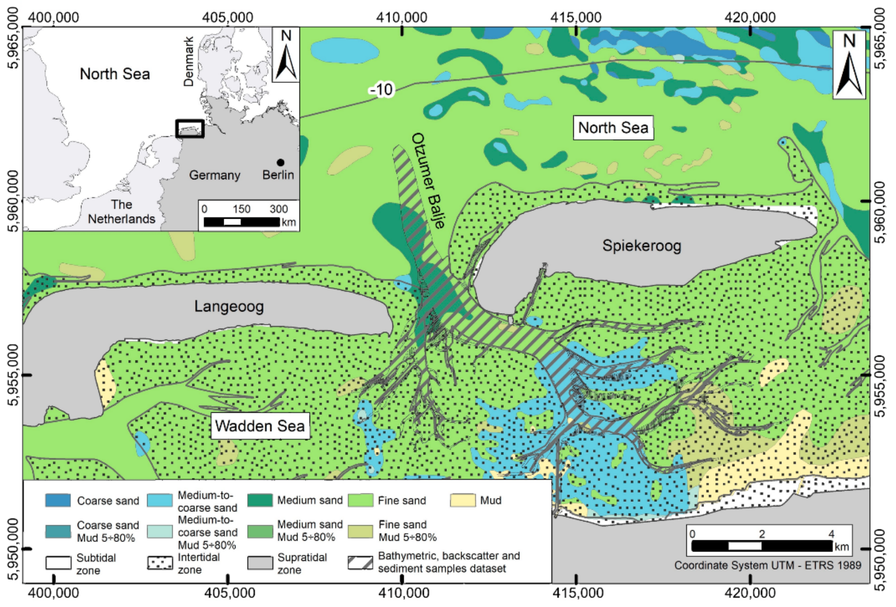
2. Study Area

The Wadden Sea is the largest mesotidal system in the world, extending along the coasts of the Netherlands, Germany, and Denmark [2]. It is a series of 39 distinctive tidal basins made of salt marshes, tidal flats, tidal gullies, barrier islands, and ebb-tidal deltas. The Frisian barrier islands separate the Wadden Sea from the North Sea. They result from coastal depositional processes occurring during the Holocene sea-level rise [10]. Between them, the strong currents of tidal flows generate tidal inlets up to 30 m deep (Figure 1). The Wadden Sea is mainly made of a Late Holocene succession that is, on average, up to 20 m thick [11]. It consists of a basal peat covered by marine and brackish sandy deposits, silt, clay, and intercalated peat lenses. The surficial sediments mainly consist of fine to coarse sand. The mud fraction is generally lower than 5% in the tidal channels and in the North Sea area, increasing towards the intertidal sectors (Figure 1). A gravel fraction is rarely present in few areas of the North Sea [12,13]. Holocene deposits overlay a Pleistocene succession that is, on average, up to 50 m thick. It consists of fluvial and glaciofluvial deposits of sand, silt, and clay related to the glacial and interglacial Pleistocene stages [11].

Subtidal areas of the Otzumer Balje inlet are made of fine to coarse sands [14,15]. Waves and tidal currents steadily mobilize surficial sediments and generate a continuous sediment exchange between flood deltas, channels, and ebb deltas [16,17]. Extended small to large sand waves characterize the area, with heights up to 6 m and wavelengths up to 120 m [18]. Currents induce erosive processes and generate steep scarps on the channel slopes related to the presence of peat, cohesive clay, or consolidated coarse sand layers [11,18].

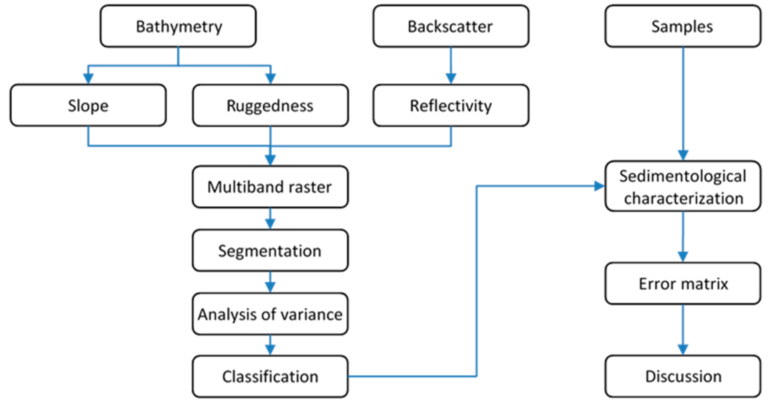
3. Materials and Methods

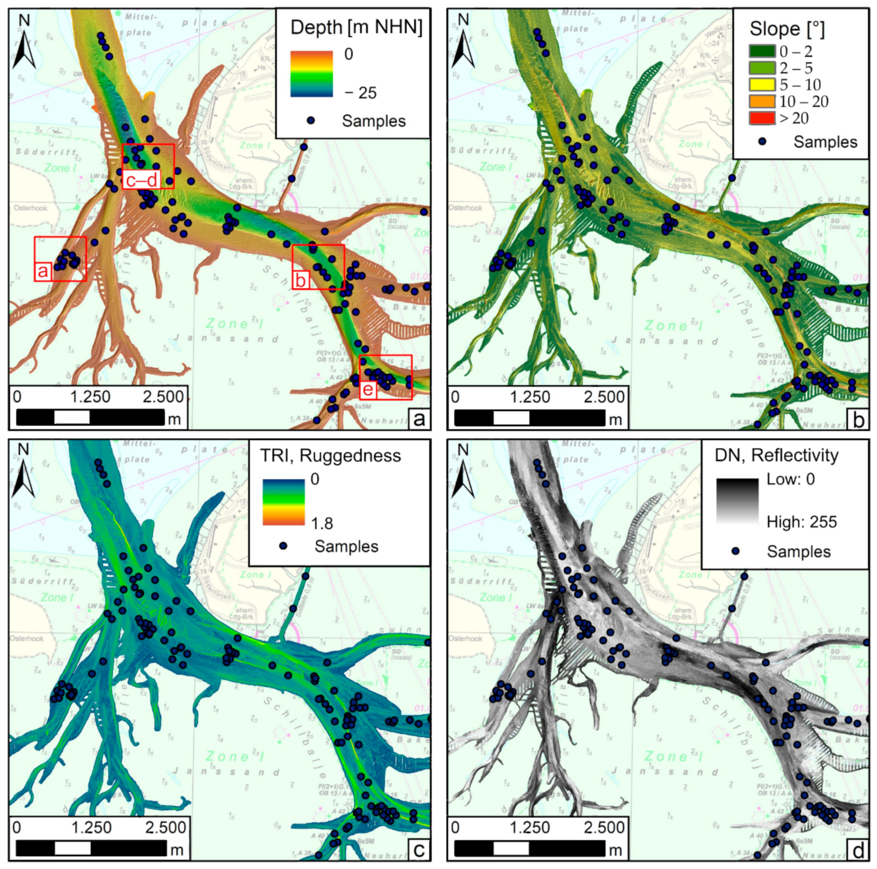
3.1. Datasets

This study combined full-coverage, hydro-acoustic data and ground truths (Figure 2) collected in 2014 over an area of approximately 19 km², with a water depth from 1.5 up to 25 m.

Bathymetric and backscatter data were collected by the NLWKN owned survey vessel Nynorderoog equipped with a hull-mounted Kongsberg EM3002D multibeam echosounder, operating at a frequency of 300 kHz and fully compensated for vessel motion. Sound velocity profiles were measured every 2 h to account for the hydrology effects. The Real-Time Kinematic (RTK) positioning technique and SAtellite POsitioning Service (SAPOS^®) provided position and elevation. Raw data were processed with QPS QINSy software (ver. 8.10) by considering sound velocity variations, tides, and basic quality control.

Over 130 sediment samples were collected by the NLWKN owned research vessel Burchana equipped with a 50 l Van Veen grab. The number and position of samples were planned based on a preliminary interpretation of bathymetry and reflectivity to ground-truth the different acoustic sectors and to verify substrate changes along the main breaks of slope (Figure 3). The positions of collected samples were assumed the planned ones, although they may differ because of the drift of both vessel and grab due to tidal currents. The difference between planned and actual sampling points was estimated in a second time, based on a further set of samples collected in 2015 whose position was pinpointed by means of an Ultra-Short BaseLine (USBL) underwater positioning system.

The sample analysis was firstly performed on board through a qualitative description of the sample surface, particle size, colour, consolidation or cohesion rate, and biogenic content. A sub-sample was collected to perform laboratory sieve analyses. Particle-size distribution and sample statistics were computed by means of the Gradistat software (ver. 8) [19]. Sediments were classified according to the Folk classification [20] simplified to four classes as proposed by BSH [21], and the sand fractions were classified according to the Figge classification [12].

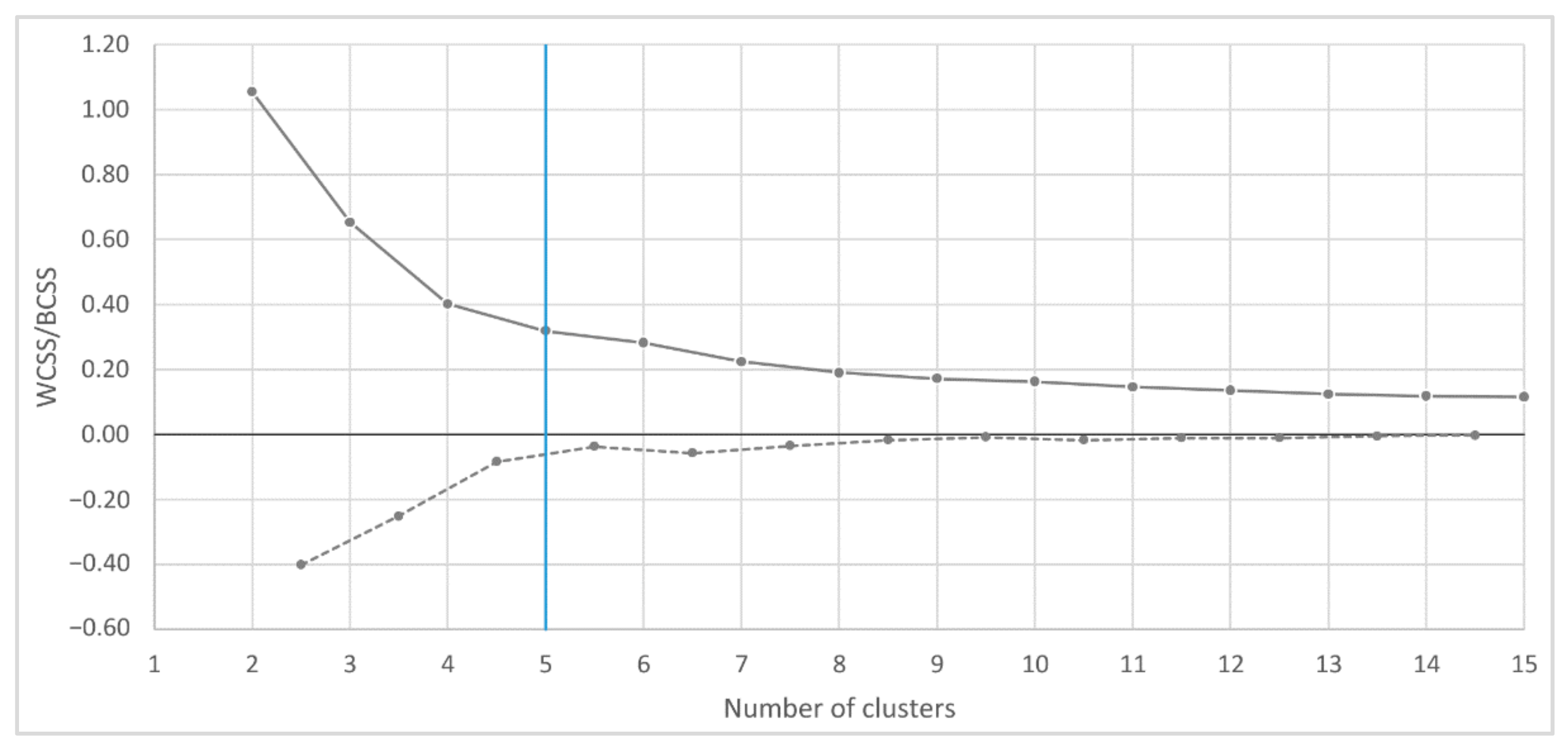
3.2. Segmentation and Classification of Hydro-Acoustic Data

Bathymetrical acoustic data were gridded to a 1 m cell size Digital Elevation Model (DEM, Figure 3). Backscatter was processed by means of QPS FMGeocoder software (ver. 7.4) for radiometric and geometric corrections [5,22]. Mosaics were generated as greyscale images with a cell size of 1 m (Figure 3), and reflectivity intensities were expressed in Digital Numbers (DN) from 0 to 255 [9]. Slope and ruggedness were derived from the DEM using ESRI ArcGIS 10.5^TM tools (Figure 3). The slope computation was based on a 3 × 3 cell neighbourhood around the centre cell and expressed as an angle to the horizontal in degrees. Ruggedness was calculated for each grid cell by computing the sum change in elevation between the centre cell and its 5 × 5 neighbour grid cells, and expressed as a Terrain Ruggedness Index (TRI) [23].

Reflectivity, slope, and ruggedness were combined into a multiband raster since they are good proxies for sediment types, substrate variations, and geomorphological processes [9,18,24].

The resulting raster was the input of the object-based approach, of which extracts feature from images based on groups of pixels. The process segments the images into similar objects (groupsof pixels), classifies them into n classes, and characterizes the classes based on ground truths [25]. ESRI ArcMap 10.5^TM was used to carry out segmentation and classification. The segmentation tool is based on the Mean Shift approach. The technique uses a moving window that calculates an average pixel value to determine which pixels should be included in each segment. As the window moves over the image, it iteratively recomputes the value to make sure that each segment is suitable. The result is a grouping of adjacent pixels that have similar spectral characteristics into a segment characterized by an average value [26]. The segmented raster was classified using the ISO-cluster unsupervised classification. The process group segments with similar statistical properties into a user-specified number of distinct clusters [27]. The choice of the optimal number of clusters was a critical step of the entire process, since it was previously unknown how many substrate types were actually present and how many of them could be efficiently identified by acoustic data. The question was here managed through the analysis of variance, which uses the Within-Clusters Sum of Squares (WCSS) and the Between-Clusters Sum of Squares (BCSS) to check whether two or more groups of data differ significantly among themselves [8]. The WCSS and the BCSS values were calculated for a number of clusters ranging from 2 up to 15 according to the equations:

$${\mathrm{WCSS}}_j={{\displaystyle \sum }}_{k=1}^j{n}_k{\sigma }_k^2\hspace{1em}\hspace{1em}{ \mathrm{BCSS}}_j={{\displaystyle \sum }}_{k=1}^j{n}_k{\left({\mu }_k-M\right)}^2,$$

(1)

where j is the number of clusters in each set, k is the number of the considered cluster, n_k, σ²_k, and μ_k are, respectively, the number of values, the variance, and the mean value within the k cluster, and M is the mean of all values [28]. The optimal number of clusters for the ISO-cluster classification was determined using the elbow method by plotting the WCSS/BCSS ratios against the number of clusters [8,29]. The aim was to define the minimum number of clusters such that the total intra-cluster variation (WCSS) was minimized and the between-cluster variation (BCSS) was maximized. This number was graphically identified by the bend in the WCSS/BCSS plot (Figure 4). Adding more clusters resulted into a flattening of the curve and did not provide a better modelling of the data.

The result of the ISO-cluster was a classified image, which still did not contain any information about substrates. Statistics of reflectivity, slope, and ruggedness within each cluster were plotted on box-plot diagrams, explicitly showing the median and the extremes, as well as the variability around the median [30].

3.3. Seabed Characterization and Validation of Results

Sediment samples and particle-size analyses were used to validate the classification of the acoustic data. Ground-truth locations were plotted in ESRI ArcGIS 10.5^TM and substrate information were joined to the ISO-cluster classified image. The sediment characterization of each cluster was based on the frequency of occurrence of sediment types. The classification accuracy was investigated by means of an error matrix, which reports the overall thematic map accuracy, the representation, the purity, and the Kappa coefficient of agreement [31,32]. The overall accuracy depicts the percentage of correctly allocated cases and is computed by dividing the sum of all correct classifications by the total number of samples. Representation is how often the collected sediments are correctly shown on the classified map and expresses the probability that a certain substrate of an area of the seabed is classified as such. It is calculated by dividing the number of accurately classified reference sites by the total number of reference sites for that cluster. Purity is how often the granulometric class on the map is actually present on the ground, and is referred to as reliability. It is calculated by dividing the total number of correct classifications in a particular cluster by the total number of samples in the same. Cohen’s Kappa coefficient (k) takes into account the possibility of the agreement occurring by chance, and evaluates the reliability of the performed classification compared to randomly assigned values [31].

The last step of this study was the punctual analysis of the incorrectly allocated cases, carried out through the critical evaluation of seabed geomorphological features, samples position accuracy, and adopted classification systems.

4. Results

4.1. Seabed Segmentation and Classification

The analysis of variance performed on the segmented raster shows that the WCSS/BCSS ratio quickly decreases as the number of clusters increases from 2 to 5, and becomes approximately constant for more than six clusters. Accordingly, the gradient of the curve approaches zero by increasing the clusters number (Figure 4). Therefore, the segments can be fairly grouped into five clusters. A higher number does not provide further details to the classification process.

The statistical analysis of each cluster outlines that reflectivity has a good discriminatory power and properly separates Clusters 2 and 4, which have mean values of 117 and 147 DN. On the other hand, Clusters 1, 3, and 5 show a similar mean reflectivity of about 130 DN (Figure 5). Slope and ruggedness substantially contribute to clear characterization of Cluster 5, since a mean value of 15.3° and a TRI of 0.61 highlight a steeper and more complex morphology compared to other clusters. In the same way, even if Clusters 1 to 4 have similar slope and ruggedness values, Cluster 3 presents the highest mean and the largest range due to a more complex morphology. On the other hand, Cluster 1 has lower mean values and smaller ranges than other clusters (Figure 5).

4.2. Sediment Analysis

Sediments range from mud and sandy mud to coarse sediments (Figure 6) with the gravel fraction made of mollusc-shell debris. Mud and sandy mud represent 20% of collected samples, including muddy sand, sandy mud, and mud. The mud content ranges from 10 to 95% (Figure 6). Sandy sediments correspond to 35% of collected samples and are mainly made of fine and medium sand, with a few samples made of medium-to-coarse and coarse sand (Figure 6). Coarse sediments are the 33% of collected samples. They are made of an association of sand and contain up to 40% of mollusc-shell debris. The sand fraction ranges from fine to coarse (Figure 6). Organic peat and very cohesive clay were collected close to the very steep slopes and constitute 12% of all samples.

4.3. Seabed Characterization

The comparison between samples and classified acoustic data shows that 31 samples belong to Cluster 1. Twenty-three of them are mud and sandy mud (

Table 1. Error matrix and accuracy coefficients. The matrix contains the number and type of sediments per cluster. Abbreviations refer to sample classes shown in Figure 6.

Ground-Truth
OBIA-Clusters	MsM	S, fS	S, mS-mcS	cSED	HS	Total	Purity
1	23	5	0	3	0	31	74.2%
2	1	30	1	3	0	35	85.7%
3	2	2	7	1	0	12	58.3%
4	3	5	0	40	0	48	83.3%
5	0	0	0	0	11	11	100.0%
Total	29	42	8	47	11	137
Representation	79.3%	71.4%	87.5%	85.1%	100.0%
Overall Accuracy = 81.0%				Kappa Coefficient = 0.74

), with the sand fraction mostly made of fine sand. The remaining eight samples are fine sands and coarse sediments characterized by a medium to coarse sand fraction never exceeding 15% (Figure 7). Slope and ruggedness depict a flat and morphologically homogeneous area characterized by small sand waves with heights up to 10 cm covering small areas. Most of the surface is characterized by the absence of bedforms (Figure 7). The classification of Cluster 1 as mud and sandy mud results in a representation of 79.3% and a purity of 74.2% (Table 1).

Cluster 2 contains 30 samples of well-sorted fine sands, which represent 86% of all grab samples collected within this cluster (Table 1). Remaining samples consist of coarse sediments with a gravel fraction lower than 10% and a fine sand fraction, medium sand, and mud and sandy mud (Figure 7). The morphology is characterized by generally flat to gently sloping areas, locally covered by sand wave fields, made of small to large sand waves, with wavelengths ranging from 5 to 35 m and heights from 0.15 to 1 m (Figure 7). Cluster 2 is then classified as fine sand, with a representation of 71.4% and a purity level of 85.7% (Table 1).

Cluster 3 is the less represented one and matches quite heterogeneous sediments. Seven samples are made of medium to coarse sand (Table 1). The remaining samples consist of fine sands, mud and sandy muds, and a sample of coarse sediments (Table 1). Noticeably, this last of these presents a sand fraction of 88% (Figure 7). Morphologically, this cluster extends over flat to gently sloping areas, with a mean slope gradient of about 4°. Areas are covered by extensive small to large sand wave fields, with wavelengths ranging from 5 to 35 m and heights from 0.15 to 1 m (Figure 7). The classification of Cluster 3 as medium and medium to coarse sand results in a high representation of 87.5%. On the other hand, the cluster contains several other different sediment types, which results in a relatively low purity of 58.3% (Table 1).

Cluster 4 is effectively represented by 40 coarse sediment samples (Table 1) with a heterogeneous sand fraction ranging from fine to coarse (Figure 7). The remaining eight samples consist of fine sands, as well as mud and sandy muds. Morphologically, it extends over flat areas generally covered by small to large sand wave fields with wavelengths ranging from 5 to 35 m and heights from 0.15 to 1 m (Figure 7). The classification of Cluster 4 as coarse sediments results in high values of both representation and purity of 85.1% and 83.3%, respectively (Table 1).

Cluster 5 is definitely well-described by morphometrical parameters, with a prevalence of steep surfaces, bounded on the upper part by sharp convex breaks of slope, giving the surrounding areas a terraced morphology (Figure 7). Due to the steep gradients, the planar extension is generally small and characterized by long narrow sectors parallel to the channels. The sampling process is consequently difficult, even if all 11 samples collected close to these sectors reveal the presence of organic peat and very cohesive clay (Figure 7).

5. Discussion

5.1. Assessment of Accuracy

The seabed of a shallow and complex tidal inlet was divided into five lithologically and geomorphologically meaningful clusters. This result was achieved adopting a repeatable methodological workflow based on high-resolution multibeam data and ground truths. In accordance with the most recent studies on seabed mapping [8,33,34,35], the combination of morphometrical and hydro-acoustic features strongly increased the consistency of seafloor classification. Reflectivity was a proxy for sediment particle size and mainly contributed to the recognization of different sediment types. Artefact-reduced images allowed for quantitative analyses. In the present case, reflectivity generally increased by particle-size coarsening. An exception was the relatively high reflectivity of mud and sandy mud. The explanation is a strong bioturbation, in accordance with the earlier work by Roche et al. (2013) [36].

Morphometrical features contributed to the differentiation of clusters with similar reflectivity. Steep slopes, high ruggedness, and sharp breaks of slope clearly identify Cluster 5. The ground-truthing of this cluster was difficult due to outcrop narrowness; hence, its characterization solely based on samples was uncertain. Therefore, its geological characterization is based on the interpretation of several factors. Morphological features given by steep slopes and breaks of slope reveal the presence of a substrate harder than unconsolidated sand. The depth of Cluster 5 areas is consistent with the depth of the Holocene base [11]. Ground truths collected close to Cluster 5 generally contain peat. Consequently, Cluster 5 is classified as hard substrate, referred to the Holocene basal peat and the Upper Pleistocene sandy sediments. This interpretation is in line with stratigraphical investigations performed on similar tidal inlets of the Wadden Sea [37,38].

5.2. Analysis of Inconsistencies

The seabed classification based on acoustic data using automatic methods such as OBIA and verified by ground truths normally results in a partial agreement between acoustic clusters and gathered samples [39,40]. Inconsistencies are often observed near cluster boundaries or in areas characterized by high terrain complexity. This study provided a map with a substantial agreement between predicted clusters and ground truths, defined by an overall accuracy of 81% and a Kappa coefficient of 0.74. The punctual analysis of inconsistent cases outlined three different reasons (

Table 2. Analysis of inconsistencies between ground truths and predicted clusters. G-T = ground-truth; Predicted = clusters resulting from the OBIA verified by ground-truths according to the error matrix in Table 1; C = inconsistency due to classifications; G = inconsistency due to geomorphology; P = inconsistency due to samples position. Other abbreviations refer to sample classes shown in Figure 6.

Sample	Predicted	G-T	C	G	P	Description
otz_001	MsM, fS	S, fS	x			Similar reflectivity of S, fS and MsM, fS with bioturbation
otz_030	MsM, fS	S, fS			x	2.5 m from a S, fS area
otz_045	MsM, fS	cSED, mcS	x		x	8 m from a S, mcS area–Coarse fraction 8.6%
otz_071	MsM, fS	cSED, mcS			x	50 m from a cSED, mcS area
otz_088	MsM, fS	cSED, fS			x	13 m from a cSED area
otz_093	MsM, fS	S, fS		x		Small scaled sediment sorting on sand waves
otz_134	MsM, fS	S, fS	x			19 m from a S, fS area
otz_151	MsM, fS	S, fS	x			Similar reflectivity of S, fS and MsM, fS with bioturbation
otz_049	S, fS	MixSed, fS	x		x	Consistent sand fraction, coarse fraction 8.8%–1 m from a MsM, fS boundary
otz_077	S, fS	cSED, fS	x			Consistent sand fraction–coarse fraction 9.5%
otz_079	S, fS	cSED, fS	x			Consistent sand fraction–coarse fraction 7.4%
otz_090	S, fS	S, mS	x			fS–mS ratio very closed to the Figge boundary
otz_116	S, fS	cSED, fS	x			Consistent sand fraction–coarse fraction 9.5%
otz_010	S, mS–mcS	S, fS		x		Small scaled sediment sorting on sand waves
otz_046	S, mS–mcS	S, fS			x	13 m from a fS area
otz_084	S, mS–mcS	S, cS		x		Small scaled sediment sorting on sand waves
otz_091	S, mS–mcS	MsM, fS		x		Small sand waves on muddy layer–Classification consistent surficial sediment
otz_119	S, mS–mcS	MsM, mS		x		Small sand waves on muddy layer–Classification consistent surficial sediment
otz_142	S, mS–mcS	cSED, mcS	x		x	Collected on a boundary S, mcS. Consistent san–Coarse fraction 10%
otz_144	S, mS–mcS	S, fS		x		Small scaled sediment sorting on sand waves
otz_005	cSED, fS–cS	S, fS		x		Small scaled sediment sorting on sand waves
otz_016	cSED, fS–cS	MsM, fS			x	10 m from a MsM area
otz_033	cSED, fS–cS	S, fS		x		Small scaled sediment sorting on sand waves
otz_052	cSED, fS–cS	MsM, fS			x	5 m from a MsM area
otz_080	cSED, fS–cS	MsM, fS			x	10 m from a MsM area
otz_081	cSED, fS–cS	S, fS		x		Small scaled sediment sorting on sand waves
otz_136	cSED, fS–cS	S, fS		x		Small scaled sediment sorting on sand waves
otz_143	cSED, fS–cS	S, fS			x	17 m from a MsM area

).

The first is the not direct correspondence between boundaries derived from the clustering process and those of sediment classification systems. In particular, clusters classified as mud and sandy mud or sand contain several coarse sediment samples. However, particle size analysis unveiled a gravel fraction lower than 10%, that is, quite close to the boundary between sand and coarse sediments in the Folk classification [20] (Figure 7). The gravel fraction was made of small shells or shell fragments with a flat shape and included in a sandy matrix, which resulted in surface micro-ruggedness and an acoustic behaviour quite similar to that of fine sediments, as already observed by Goff et al. (2004) [41]. Furthermore, several well-sorted fine sands were classified as mud and sandy mud in the image analysis. All considered samples had a mean mud content of 2.2% with a maximum of 7%. Even if such content is quite low, it must be considered that these samples have cohesive behaviour, which confers very low ruggedness and relatively low reflectivity to the seabed surface. In addition, the sampling procedure by means of the Van Veen grab tends to underestimate the mud fraction, since part of the finest fraction can be lost in the water column during grab recovery [9]. Such observations outlined that most of the errors were located close to the Folk boundaries between sand and neighbouring classes. The reason is that the commonly used sediment classification systems were created as a function of particle size [12,20], making approximations in acoustic data classification actually unavoidable, especially in areas with slight differences between sediment types.

The second reason for inconsistency is the geomorphology of the seabed. Over 30% of non-matching samples are located on extended small to large sand wave fields. These bedforms generally present sediment sorting and particle size differentiation between crests and troughs [42,43,44,45,46,47,48,49]. In the OBIA classification, the segment size is generally set large enough to filter out small segments and provide a clear map. It implies that crests and troughs can be included in the same segment and classified as the same seabed type, even if composed by slightly different sediments (Figure 7). Consequently, the smoothness generated by pixel grouping does not perfectly match the punctual information provided by grab samples, which can refer to the crests or to the troughs. In the present case, the influence of bedforms on the sediment sorting explains most of the inconsistencies observed within Clusters 3 and 4, both widely covered by sand waves.

The last reason of inconsistency was the position accuracy of ground truths. Concerning the samples presented in this work, the grab positions were considered the planned ones. However, the vessel drift due to tidal currents and wind makes the positioning on the planned point rather hard. In addition, the strong currents shift the grab from the vertical, making the positioning of the sample even more uncertain. The distance between the planned positions and the actual sampled points was measured by means of an USBL system on a sample dataset collected in 2015 by the same vessel and under the same environmental conditions [50]. The mean value is about 25 m, with a maximum of 50 m (Figure 8).

They are consistent with the distances measured between some incorrectly allocated samples and neighbouring clusters actually characterized by the same sediment type (Table 2), which points out the inaccuracy of the positioning method.

6. Conclusions

This study provides a practical application of objective mapping methods within institutional extended mapping programs. The combination of geomorphometric analysis, reflectivity, and ground truths is a consistent approach for producing accurate and reproducible maps of the spatial sediment distribution. Results show that automatic methods provide consistent products, allow to keep track of the mapping process, and reduce production time. However, the application on a complex coastal area, made of different types of sandy sediments, which cover relatively small seabed portions and are often shaped by bedforms, outlines some crucial aspects highlighted by the inconsistencies between ground truths and expected sediment classes.

The punctual analysis of inconsistency cases reveals that they are commonly placed close to the boundaries between similar sediment types. The reason is that limits set by sediment classifications are based on the particle size distribution, and do not necessarily match cluster boundaries derived by hydro-acoustic data, which depend on the acoustic properties of sediments. Further inconsistencies are generated by the presence of peculiar bedforms, such as large and medium sand waves. Even though the interpretation of hydro-acoustic data shows large, lithologically homogeneous portions of seabed, they actually present sediment sorting due to the presence of sand waves. Lastly, the uncertain position of samples becomes of critical importance when working in complex areas characterized by high spatial variability of seabed and strong drift during sampling operations.

In conclusion, this study outlines that, even if the mapping process should be more automatic and objective, it remains an interactive procedure where the various sources of uncertainty have to be critically investigated. The knowledge of general geological information, as well as a detailed geomorphological characterization, are of primary importance in results evaluation. Gaps between classification schemes and outputs of classification algorithms have to be considered. Despite the continuous scientific progresses, their correlation is still a wide field of research to explore and develop. The successful application of automatic mapping will take great advantage of the availability of high-quality hydro-acoustics, as well as accurate ground-truth data.

References

- Buhl-Mortensen, L.; Buhl-Mortensen, P.; Dolan, M.F.J.; Holte, B. The MAREANO Programme—A full coverage mapping of the norwegian off-shore benthic environment and fauna. Mar. Biol. Res. 2015, 11, 4–17. [Google Scholar] [CrossRef]
- Kloepper, S.; Baptist, M.J.; Bostelmann, A.; Busch, J.A.; Buschbaum, C.; Gutow, L.; Janssen, G.; Jensen, K.; Jørgensen, H.P.; de Jong, F.; et al. Wadden Sea Quality Status Report 2017; Common Wadden Sea Secretariat: Wilhelmshaven, Germany, 2017; Available online: https://qsr.waddensea-worldheritage.org/reports/subtidal-habitats (accessed on 11 February 2020).
- Kaskela, A.; Kotilainen, A.; Alanen, U.; Cooper, R.; Green, S.; Guinan, J.; van Heteren, S.; Kihlman, S.; Van Lancker, V.; Stevenson, A.; et al. Picking up the pieces—Harmonising and collating seabed substrate data for European Maritime Areas. Geosciences 2019, 9, 84. [Google Scholar] [CrossRef]
- Lucieer, V.; Barrett, N.; Butler, C.; Flukes, E.; Ierodiaconou, D.; Ingleton, T.; Jordan, A.; Monk, J.; Meeuwig, J.; Porter-Smith, R.; et al. A seafloor habitat map for the Australian continental shelf. Sci. Data 2019, 6, 120. [Google Scholar] [CrossRef] [PubMed]
- Beaudoin, J.; Hughes Clarke, J.E.; Van den Ameele, E.J.; Gardner, J.V. Geometric and radiometric correction of multibeam backscatter derived from Reson 8101 systems. In Proceedings of the Canadian Hydrographic Conference, Toronto, ON, Canada, 15–19 April 2002. [Google Scholar]
- Lurton, X. An Introduction to Underwater Acoustics. Principles and Applications, 2nd ed.; Springer: Berlin/Heidelberg, Germany, 2010; p. 680. [Google Scholar]
- Brown, C.J.; Todd, B.J.; Kostylev, V.E.; Pickrill, R.A. Image-based classification of multibeam sonar backscatter data for objective surficial sediment mapping of Georges Bank, Canada. Cont. Shelf Res. 2011, 31, 110–119. [Google Scholar] [CrossRef]
- Ismail, K.; Huvenne, V.A.; Masson, D.G. Objective automated classification technique for marine landscape mapping in submarine canyons. Mar. Geol. 2015, 362, 17–32. [Google Scholar] [CrossRef]
- Diesing, M.; Green, S.L.; Stephens, D.; Lark, R.M.; Stewart, H.A.; Dove, D. Mapping seabed sediments: Comparison of manual, geostatistical, object–based image analysis and machine learning approaches. Cont. Shelf Res. 2014, 84, 107–119. [Google Scholar] [CrossRef]
- Lüders, K. Die Entstehung der ostfriesischen Inseln und der Einfluß der Dünenbildung auf den geologischen Aufbau der ostfriesischen Küste. Probl. Küstenforschung Südlichen Nordseegebiet 1953, 5, 5–14. [Google Scholar]
- Streif, H. Sedimentary record of Pleistocene and Holocene marine inundations along the North Sea coast of Lower Saxony, Germany. Quat. Int. 2004, 112, 3–28. [Google Scholar] [CrossRef]
- Figge, K. Begleitheft zur Karte der Sedimentkartierung in der Deutschen Bucht 1:250.000 Nr. 2900; Bundesamt für Seeschifffahrt und Hydrographie BSH: Hamburg, Germany, 1981. [Google Scholar]
- Zeiler, M.; Schwarzer, K.; Ricklefs, K. Seabed morphology and sediment dynamics. Küste 2008, 74, 31–44. [Google Scholar]
- Flemming, B.W.; Davis, R.A., Jr. Holocene evolution, morphodynamics and sedimentology of the Spiekeroog barrier island system (southern North Sea). Senckenbergiana Marit. 1994, 24, 117–155. [Google Scholar]
- Son, C.S.; Flemming, B.W.; Bartholomä, A. Evidence for sediment recirculation on an ebb–tidal delta of the East Frisian barrier–island system, southern North Sea. Geo Mar. Lett. 2011, 31, 87–100. [Google Scholar] [CrossRef]
- Ladage, F.; Meyer, C.; Stephan, H.J.; Niemeyer, H.D. Morphologische Entwicklung im Seegat Otzumer Balje und seinem Einzugsgebiet. In Untersuchungsbericht 2/2006; NLWKN-Forschungsstelle Küste: Norderney, Germany, 2006; p. 63. [Google Scholar]
- Meyer, C. Morphodynamische Analysen im Bereich des Norderneyer Seegats und seines Einzugsgebietes. In Untersuchungsbericht 1/2014; NLWKN-Forschungsstelle Küste: Norderney, Germany, 2014; p. 23. [Google Scholar]
- Mascioli, F.; Bremm, G.; Bruckert, P.; Tants, R.; Dirks, H.; Wurpts, A. The contribution of geomorphometry to the seabed characterization of tidal inlets (Wadden Sea, Germany). Z. Geomorphol. 2017, 61, 179–197. [Google Scholar] [CrossRef]
- Blott, S.J.; Pye, K. Gradistat: A grain size distribution and statistics package for the analysis of unconsolidated sediments. Earth Surf. Process. Landf. 2001, 26, 1237–1248. [Google Scholar] [CrossRef]
- Folk, R.L. The distinction between grain size and mineral composition in sedimentary–rock nomenclature. J. Geol. 1954, 62, 344–359. [Google Scholar] [CrossRef]
- Bundesamt für Seeschifffahrt und Hydrographie. Anleitung zur Kartierung des Meeresbodens Mittels Hochauflösender Sonare in den Deutschen Meeresgebieten; Bundesamt für Seeschifffahrt und Hydrographie BSH: Hamburg, Germany, 2016; p. 147. [Google Scholar]
- Fonseca, L.; Calder, B. Geocoder: An efficient backscatter map constructor. In Proceedings of the U.S. Hydrographic Conference, San Diego, CA, USA, 29–31 March 2005. [Google Scholar]
- Riley, S.J.; De Gloria, S.D.; Elliot, R. A terrain ruggedness index that quantifies topographic heterogeneity. Int. J. Sci. 1999, 5, 23–27. [Google Scholar]
- Miccadei, E.; Mascioli, F.; Piacentini, T. Quaternary geomorphological evolution of the Tremiti Islands (Puglia, Italy). Quat. Int. 2011, 233, 3–15. [Google Scholar] [CrossRef]
- Lucieer, V. Object-oriented classification of side scan sonar data for mapping benthic marine habitats. Int. J. Remote Sens. 2008, 29, 905–921. [Google Scholar] [CrossRef]
- Comaniciu, D.; Meer, P. Mean shift: A robust approach toward feature space analysis. IEEE Trans. Pattern Anal. Mach. Intell. 2002, 24, 603–619. [Google Scholar] [CrossRef]
- Richards, J.A. Remote Sensing Digital Image Analysis: An Introduction; Springer: Berlin/Heidelberg, Germany, 1986; p. 281. [Google Scholar]
- Forgy, E.W. Cluster analysis of multivariate data: Efficiency versus interpretability of classifications. Biometrics 1965, 21, 768–769. [Google Scholar]
- Charrad, M.; Ghazzali, N.; Boiteau, V.; Niknafs, A. NbClust: An R package for determining the relevant number of clusters in a data set. J. Stat. Softw. 2014, 61, 1–36. [Google Scholar] [CrossRef]
- Williamson, D.F.; Parker, R.A.; Kendrick, J.S. The box plot: A simple visual method to interpret data. Ann. Intern. Med. 1989, 110, 916–921. [Google Scholar] [CrossRef] [PubMed]
- Cohen, J. A coefficient of agreement for nominal scales. Educ. Psychol. Meas. 1960, 20, 37–46. [Google Scholar] [CrossRef]
- Landis, J.R.; Koch, G.G. The measurement of observer agreement for categorical data. Biometrics 1977, 33, 159–174. [Google Scholar] [CrossRef]
- Micallef, A.; Le Bas, T.P.; Huvenne, V.A.; Blondel, P.; Hühnerbach, V.; Deidun, A. A multi-method approach for benthic habitat mapping of shallow coastal areas with high-resolution multibeam data. Cont. Shelf Res. 2012, 39–40, 14–26. [Google Scholar] [CrossRef]
- Mitchell, P.J.; Downie, A.-L.; Diesing, M. How good is my map? A tool for semi-automated thematic mapping and spatially explicit confidence assessment. Environ. Model. Softw. 2018, 108, 111–122. [Google Scholar] [CrossRef]
- Linklater, M.; Ingleton, T.C.; Kinsela, M.A.; Morris, B.D.; Allen, K.M.; Sutherland, M.D.; Hanslow, D.J. Techniques for classifying seabed morphology and composition on a subtropical–temperate continental shelf. Geosciences 2019, 9, 141. [Google Scholar] [CrossRef]
- Roche, M.; Degrendele, K.; De Mol, L. Constraints and limitations of multibeam echosounders Backscatter Strength measurements for monitoring the seabed. Surveyor and geologist point of view. In Proceedings of the GeoHab Conference, Rome, Italy, 6–10 May 2013. [Google Scholar]
- Bartholomä, A.; Capperucci, R.M.; Bungenstock, F.; Schaumann, R.M.; Toerbrock, L.; Enters, D.; Wehrmann, A.; Drews, E. Rekonstruktion versunkener Landschaften im ostfriesischen Wattenmeer—Ergebnisse aus den geophysikalischen Messungen und Kernbohrungen im Projekt WASA. Nachr. Marschenrates 2020, 57, 61–69. [Google Scholar]
- Kunde, T. Entwicklung eines 3D-Modells für den unmittelbaren Untergrund des niedersächsischen Wattenmeergebietes am Beispiel von Norderney. Nachr. Marschenrates 2020, 57, 79–80. [Google Scholar]
- Steele, B.M.; Winne, J.C.; Redmond, R.L. Estimation and mapping of misclassification probabilities for thematic land cover maps. Remote Sens. Environ. 1998, 66, 192–202. [Google Scholar] [CrossRef]
- Diesing, M.; Mitchell, P.J.; O’Keeffe, E.; Montereale Gavazzi, G.O.A.; Le Bas, T. Limitations of Predicting Substrate Classes on a Sedimentary Complex but Morphologically Simple Seabed. Remote Sens. 2020, 12, 3398. [Google Scholar] [CrossRef]
- Goff, J.A.; Kraft, B.J.; Mayer, L.A.; Schock, S.G.; Sommerfield, C.K.; Olson, H.C.; Gulick, S.P.S.; Nordfjord, S. Seabed characterization on the New Jersey middle and outer shelf: Correlability and spatial variability of seafloor sediment properties. Mar. Geol. 2004, 209, 147–172. [Google Scholar] [CrossRef]
- Goff, J.A.; Olson, H.C.; Duncan, C.S. Correlation of side-scan backscatter intensity with grain-size distribution of shelf sediments, New Jersey margin. Geo Mar. Lett. 2000, 20, 43–49. [Google Scholar] [CrossRef]
- Passchier, S.; Kleinhans, M.G. Observations of sand waves, megaripples, and hummocks in the Dutch coastal area and their relation to currents and combined flow conditions. J. Geophys. Res. 2005, 110, 15. [Google Scholar] [CrossRef]
- Svenson, C.; Ernstsen, V.B.; Winter, C.; Bartholomä, A.; Hebbeln, D. Tide–driven sediment variations on a large compound dune in the Jade tidal inlet channel, Southeastern North Sea. J. Coast. Res. 2009, 56, 361–365. [Google Scholar]
- Lamarche, G.; Lurton, X.; Verdier, A.-L.; Augustin, J.-M. Quantitative characterization of seafloor substrate and bedforms using advanced processing of multibeam backscatter—Application to the Cook Strait, New Zealand. Cont. Shelf Res. 2011, 31, 93–109. [Google Scholar] [CrossRef]
- Van Oyen, T.; Blondeaux, P.; Van den Eynde, D. Sediment sorting along tidal sand waves: A comparison between field observations and theoretical predictions. Cont. Shelf Res. 2013, 63, 23–33. [Google Scholar] [CrossRef]
- Papili, S.; Jenkins, C.; Roche, M.; Wever, T.; Lopera, O.; Van Lancker, V. Influence of shells and shell debris on backscatter strength: Investigation using modeling, sonar measurements and sampling on the Belgian continental shelf. Proc. Inst. Acoust. 2015, 37, 304–310. [Google Scholar]
- Winter, C.; Lefebvre, A.; Becker, M.; Ferret, Y.; Ernsten, V.B.; Bartholdy, J.; Kwoll, E.; Flemming, B. Properties of active tidal bedforms. In Proceedings of the Marine and River Dune Dynamics Conference, MARID V, North Wales, UK, 4–6 April 2016. [Google Scholar]
- Koop, L.; Amiri-Simkooei, A.; van der Reijden, K.J.; O’Flynn, S.; Snellen, M.; Simons, D.G. Seafloor classification in a sand wave environment on the Dutch continental shelf using multibeam echosounder backscatter data. Geosciences 2019, 9, 142. [Google Scholar] [CrossRef]
- Mascioli, F.; Kunde, T. Grain size characterization of subtidal sediments of Lower Saxony. In Forschungsbericht 1/2017; NLWKN-Forschungsstelle Küste: Norderney, Germany, 2017; p. 24. [Google Scholar]