
Geochemical, Geological and Groundwater Quality Characterization of a Complex Geological Framework: The Case Study of the Coreca Area (Calabria, South Italy)


Abstract
1. Introduction
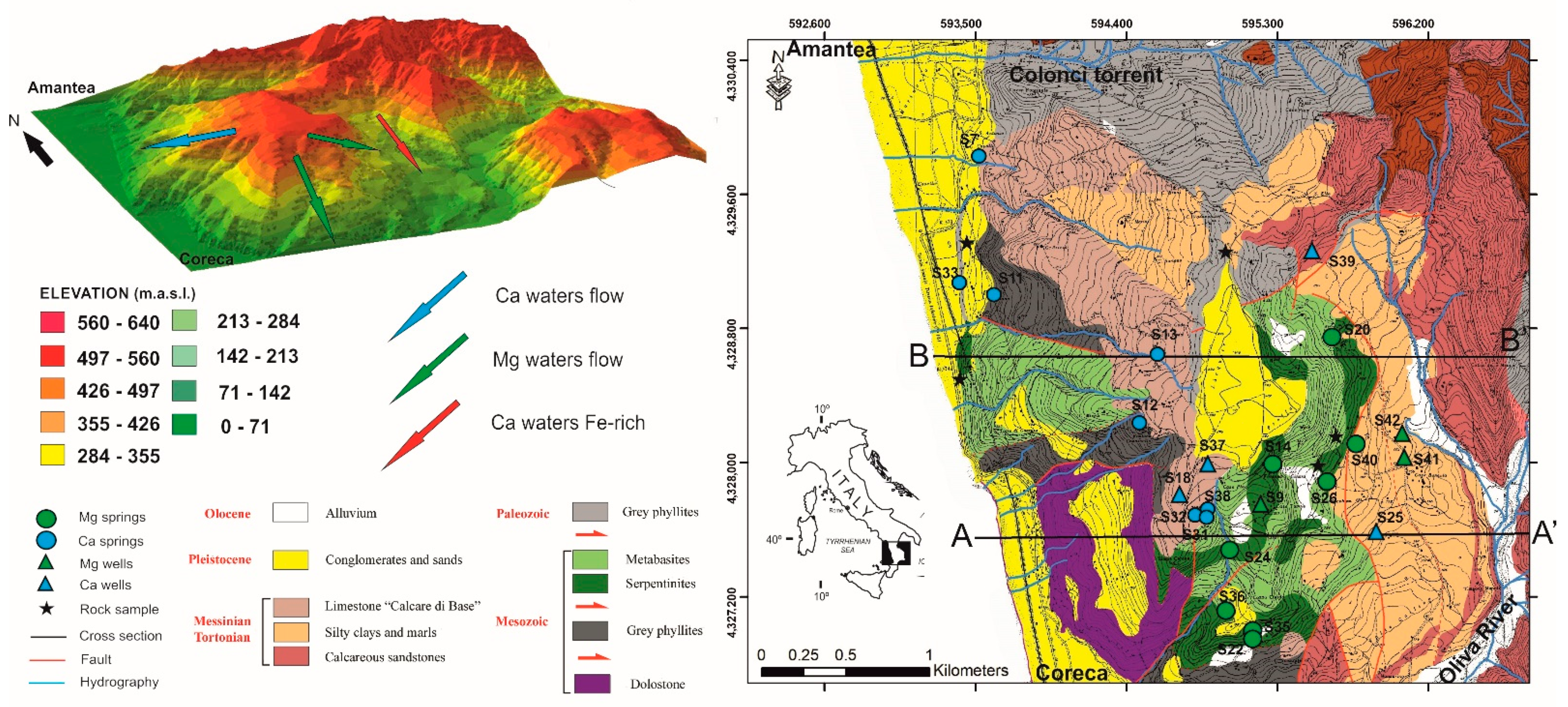
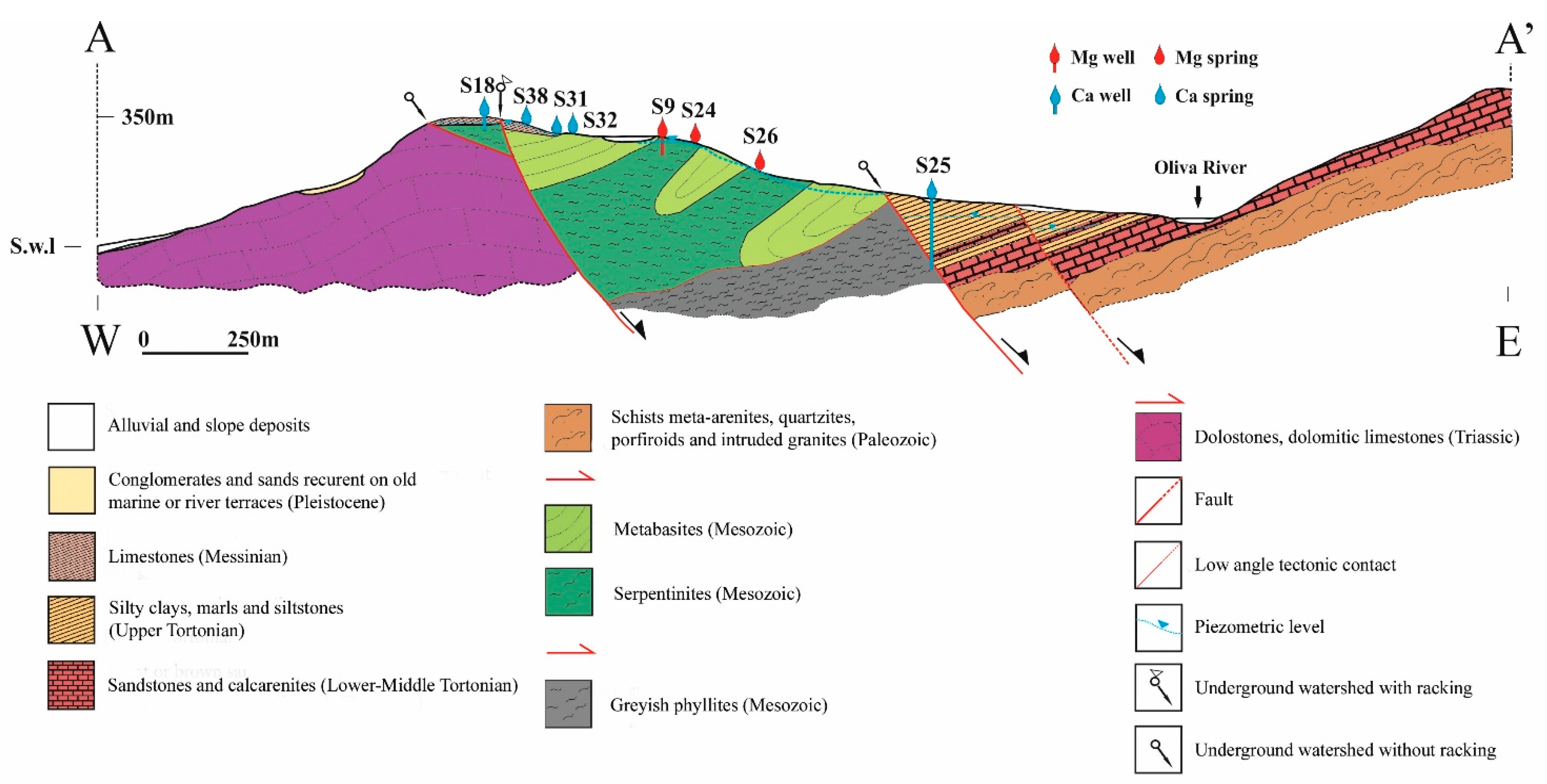
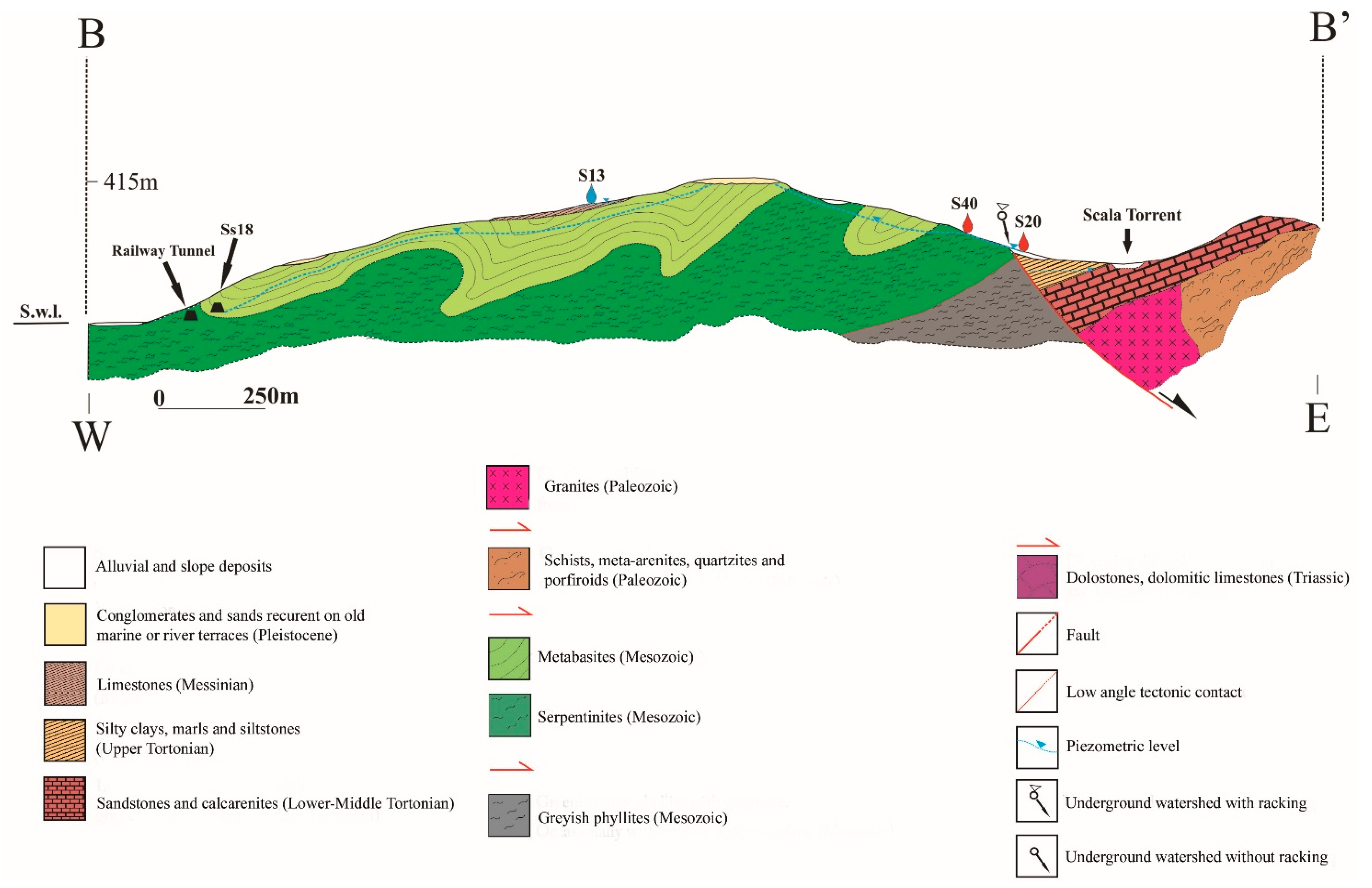
2. Geological Framework
3. Methods
4. Results and Discussion
4.1. Mineralogical Characteristics
4.2. Physical–Chemical Parameters
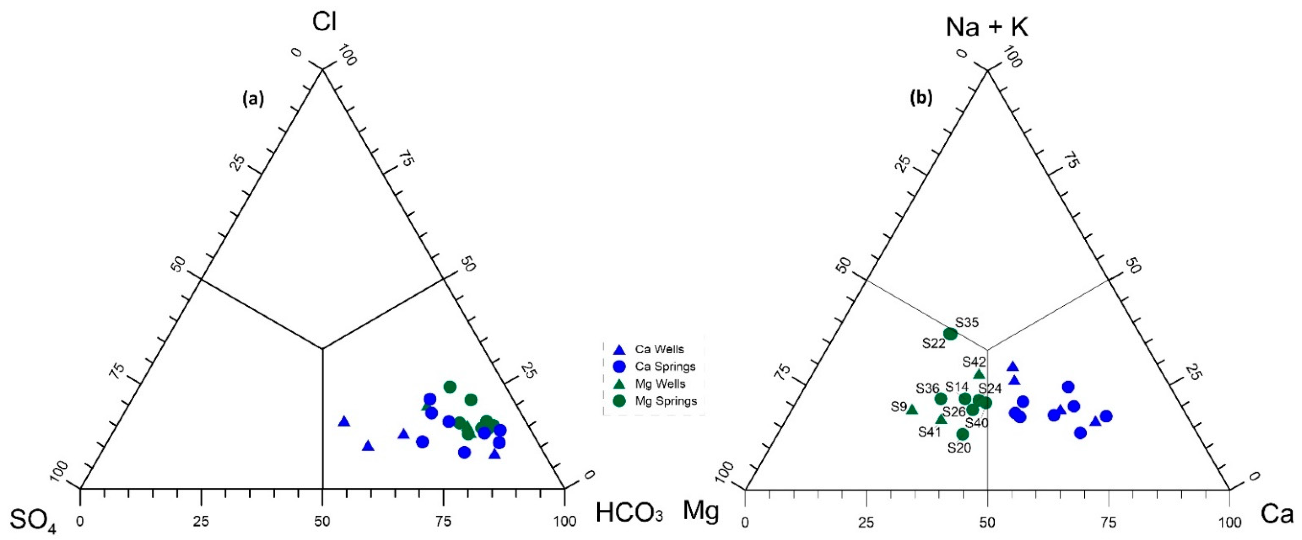
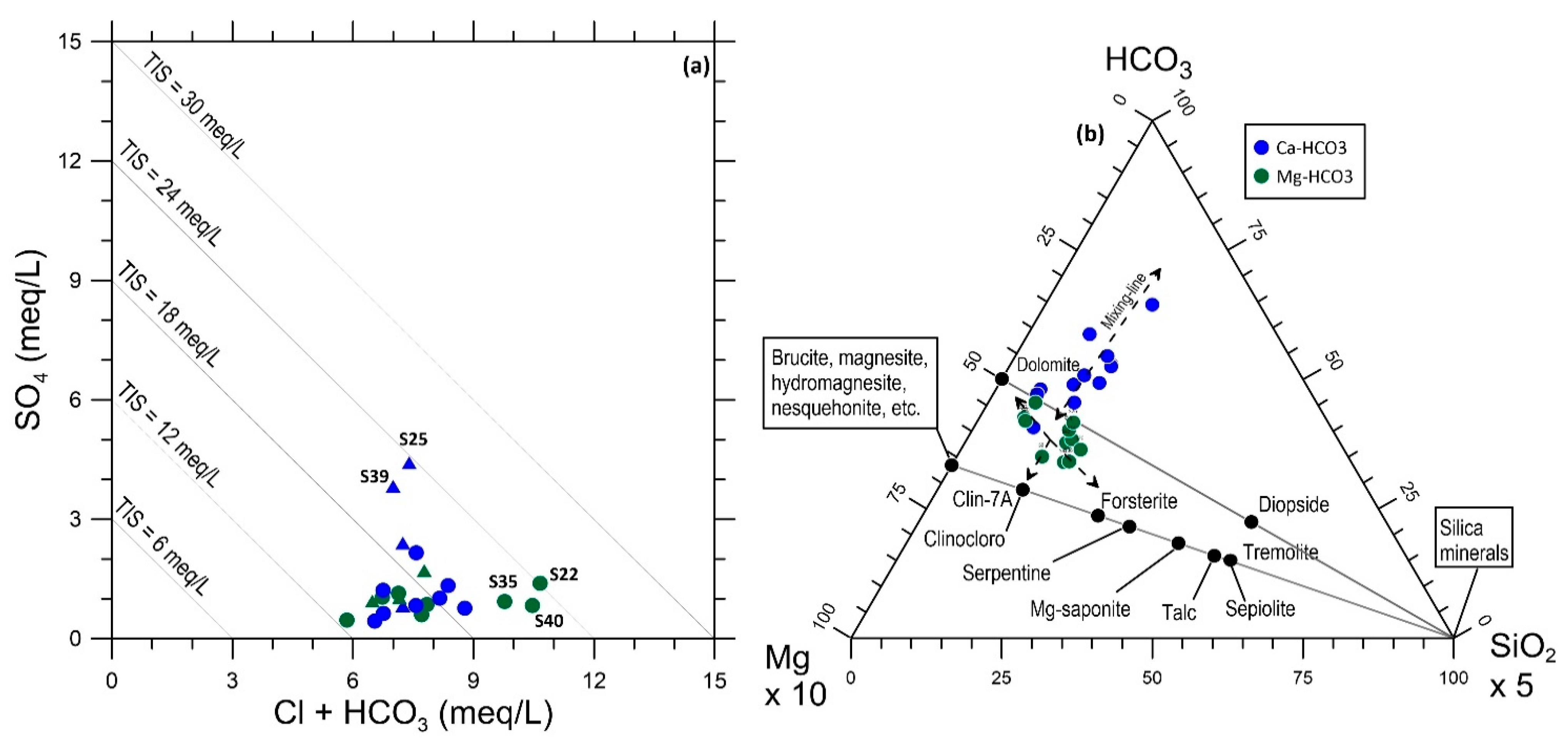
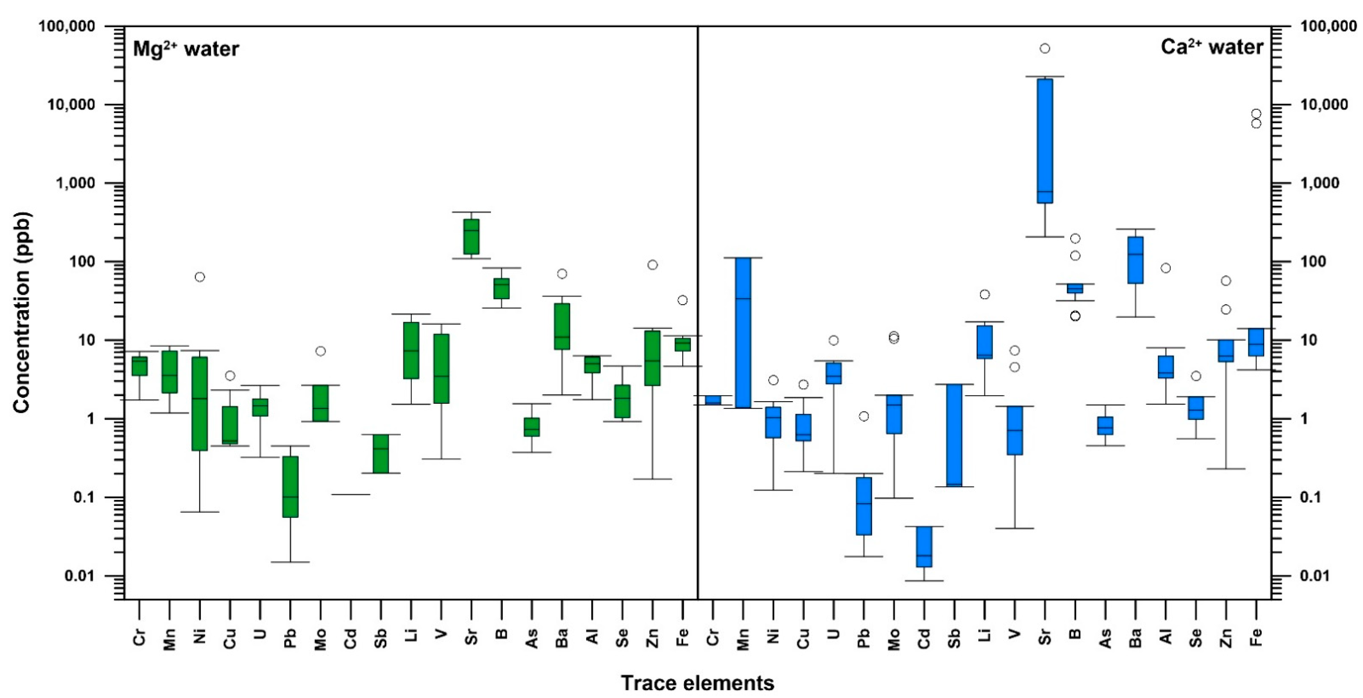
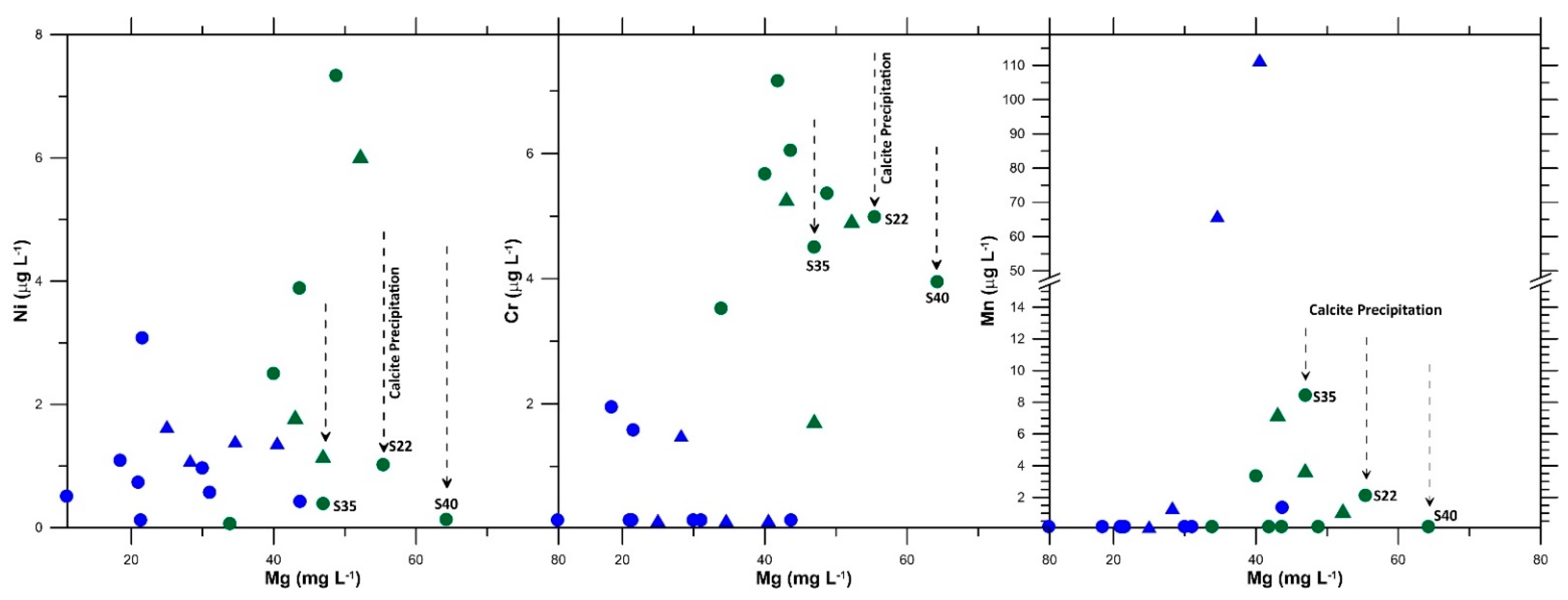
4.3. Geochemical Characteristics
4.4. Statistical Analysis
5. Groundwater Flow Interpretation
6. Water Quality
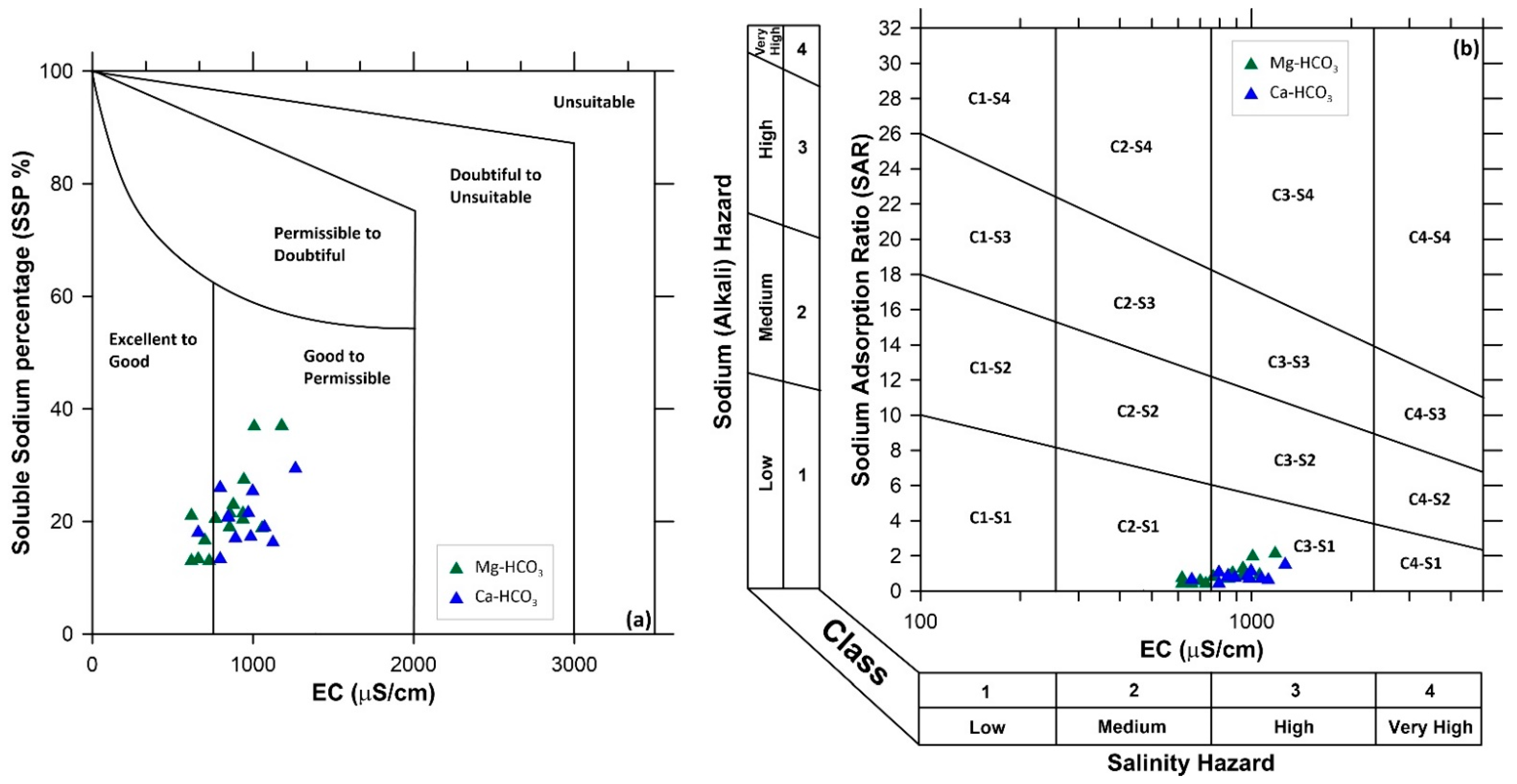
6.1. Salinity Hazard
6.2. Metal Index (MI)
7. Conclusions
Author Contributions
Funding
Institutional Review Board Statement
Informed Consent Statement
Data Availability Statement
Acknowledgments
Conflicts of Interest
References
- Appelo, C.A.J.; Postma, D. Geochemistry, Groundwaters and Pollution; A. A. Balkema: Rotterdam, The Netherlands, 1996; p. 536. [Google Scholar]
- Stumm, W.; Morgan, J.J. Aquatic Chemistry: Chemical Equilibrium and Rates in Natural Waters, 3rd ed.; Wiley: New York, NY, USA, 1996; p. 1022. [Google Scholar]
- Bocanegra, E.M.; Polemio, M.; Massone, H.E.; Dragone, V.; Limoni, P.P.; Farenga, M. A New Focus on Groundwater-Seawater Interactions. In Indicators and Quality Classification Applied to Groundwater Management in Coastal Aquifers: Mar del Plata (Argentina) and Apulia (Italy) Case Studies; Sanford, W., Langevin, C., Polemio, M., Povinec, P., Eds.; IAHS: Wallingford, UK, 2007; pp. 201–211. [Google Scholar]
- Vardè, M.; Servidio, A.; Vespasiano, G.; Pasti, L.; Cavazzini, A.; Di Traglia, M.; Rosselli, A.; Cofone, F.; Apollaro, C.; Cairns, W.R.L.; et al. Ultra-trace determination of total mercury in Italian bottled waters. Chemosphere 2019, 219, 896–913. [Google Scholar] [CrossRef]
- Vespasiano, G.; Apollaro, C. Preliminary geochemical characterization of a carbonate aquifer: The case of Pollino massif (Calabria, South Italy). Rend. Online Soc. Geol. Ital. 2016, 38, 109–112. [Google Scholar] [CrossRef]
- Vespasiano, G.; Cianflone, G.; Cannata, C.B.; Apollaro, C.; Dominici, R.; De Rosa, R. Analysis of groundwater pollution in the Sant’Eufemia Plain (Calabria—South Italy). Ital. J. Eng. Geol. Environ. 2016. [Google Scholar] [CrossRef]
- Vespasiano, G.; Notaro, P.; Cianflone, G. Water-mortar interaction in a tunnel located in the Southern Calabria (Southern Italy). Environ. Eng. Geosci. 2018, 24, 305–315. [Google Scholar] [CrossRef]
- Vespasiano, G.; Cianflone, G.; Romanazzi, A.; Apollaro, C.; Dominici, R.; Polemio, M.; De Rosa, R. A multidisciplinary approach for sustainable management of a complex coastal plain: The case of Sibari Plain (Southern Italy). Mar. Pet. Geol. 2019. [Google Scholar] [CrossRef]
- Muhammad, S.; Shah, M.T.; Khan, S. Health risk assessment of heavy metals and their source apportionment in drinking water of Kohistan region, northern Pakistan. Microchem. J. 2011, 98, 334–343. [Google Scholar] [CrossRef]
- Alaya, M.B.; Saidi, S.; Zemni, T.; Zargouni, F. Suitability assessment of deep groundwater for drinking and irrigation use in the Djeffara aquifers (Northern Gabes, south-eastern Tunisia). Environ. Earth Sci. 2014, 71, 3387–3421. [Google Scholar] [CrossRef]
- Bompoti, N.; Chrysochoou, M.; Dermatas, D. Geochemical characterization of Greek ophiolitic environments using statistical analysis. Environ. Process 2015. [Google Scholar] [CrossRef]
- Critelli, T.; Vespasiano, G.; Apollaro, C.; Muto, F.; Marini, L.; De Rosa, R. Hydrogeochemical study of an ophiolitic aquifer: A case study of Lago (Southern Italy, Calabria). Environ. Earth Sci. 2015, 74, 533–543. [Google Scholar] [CrossRef]
- Mallick, J.; Singh, C.K.; AlMesfer, M.K.; Kumar, A.; Khan, R.A.; Islam, S.; Rahman, A. Hydro-geochemical assessment of groundwater quality in Aseer Region, Saudi Arabia. Water 2018, 10, 1847. [Google Scholar] [CrossRef]
- Apollaro, C. Geochemical Modeling of Water-Rock Interaction in the Granulite Rocks of Lower Crust in the Serre Massif (Southern Calabria, Italy). Geofluids 2019. [Google Scholar] [CrossRef]
- Fehdi, C.; Rouabhia, A.; Baali, F.; Boudoukha, A. The hydrogeochemical characterization of Morsott-El Aouinet aquifer, Northeastern Algeria. Environ. Geol. 2009, 58, 1611–1620. [Google Scholar] [CrossRef]
- D.Lgs.152. Decreto Legislativo 3 Aprile 2006, n. 152, Norme in Materia Ambientale. Gazzetta Ufficiale n. 88 del 14 Aprile 2006. Supplemento Ordinario n. 96. 2006. Available online: https://www.camera.it/parlam/leggi/deleghe/06152dl.htm (accessed on 15 January 2021).
- WHO. Guidelines for Drinking-Water Quality, 4th ed.; World Health Organization: Geneva, Switzerland, 2011. [Google Scholar]
- Richards, L.A. Diagnosis and improvement of saline alkali soils. In Agriculture, 160. Handbook 60; Department of Agriculture: Washington, DC, USA, 1954. [Google Scholar]
- Kelley, W.P. Permissible composition and concentration of irrigation water. Proc. Am. Soc. Civ. Eng. 1940, 66, 607–613. [Google Scholar]
- Raghunath, H.M. Groundwater; Wiley: New Delhi, India, 1987; p. 563. [Google Scholar]
- Todd, D.K.; Mays, L.W. Groundwater Hydrology, 3rd ed.; Wiley: New York, NY, USA, 2005. [Google Scholar]
- Doneen, L.D. Notes on Water Quality in Agriculture; Department of Water Science and Engineering, University of California: Davis, CA, USA, 1964. [Google Scholar]
- Adewumi, A.J.; Anifowose, A.Y.B.; Olabode, F.O.; Laniyan, T.A. Hydrogeochemical Characterization and Vulnerability Assessment of Shallow Groundwater in Basement Complex Area, Southwest Nigeria. Contemp. Trends Geosci. 2018, 7, 72–103. [Google Scholar] [CrossRef]
- Wilcox, L.V. Classification and Use of Irrigation Waters; USDA. Circ 969: Washington, DC, USA, 1955.
- Salifu, M.; Aidoo, F.; Saah Hayford, M.; Adomako, D.; Asare, E. Evaluating the suitability of groundwater for irrigational purposes in some selected districts of the Upper West region of Ghana. Appl. Water Sci. 2017. [Google Scholar] [CrossRef]
- Rawat, K.S.; Singh, S.K.; Gautam, S.K. Assessment of groundwater quality for irrigation use: A peninsular case study. Appl. Water Sci. 2018, 8, 233. [Google Scholar] [CrossRef]
- Van Dijk, J.P.; Bello, M.; Brancaleoni, G.P.; Cantarella, G.; Costa, V.; Frixia, A.; Golfetto, F.; Merlini, S.; Riva, M.; Torricelli, S.; et al. A regional structural model for the northern sector of the Calabrian Arc (southern Italy). Tectonophysics 2000, 324, 267–320. [Google Scholar] [CrossRef]
- Critelli, S.; Muto, F.; Tripodi, V.; Perri, F.; Schattner, U. Relationships between lithospheric flexure, thrust tectonics and stratigraphic sequences in foreland setting: The Southern Apennines foreland basin system, Italy. Tectonics 2011, 2, 121–170. [Google Scholar]
- Critelli, S.; Muto, F.; Perri, F.; Tripodi, V. Interpreting provenance relations from sandstone detrital modes, southern Italy foreland region: Stratigraphic record of the Miocene tectonic evolution. Mar. Petrol. Geol. 2017, 87, 1–13. [Google Scholar] [CrossRef]
- Cirrincione, R.; Fazio, E.; Fiannacca, P.; Ortolano, G.; Pezzino, A.; Punturo, R. The Calabria-Peloritani Orogen, a composite terrane in Central Mediterranean; its overall architecture and geodynamic significance for a pre-Alpine scenario around the Tethyan basin. Progresses in Deciphering Structures and Compositions of Basement Rocks. Period. Mineral. 2015, 84, 701–749. [Google Scholar] [CrossRef]
- Bonardi, G.; Cello, G.; Perrone, V.; Tortorici, L.; Turco, E.; Zuppetta, A. The evolution of the northern sector of the Calabria–Peloritani Arc in a semiquantitative palynspastic restoration. Boll. Soc. Geol. Ital. 1982, 101, 259–274. [Google Scholar]
- Bonardi, G.; Giunta, G.; Perrone, V.; Russo, M.; Zuppetta, A.; Ciampo, G. Osservazioni sull’evoluzione dell’Arco Calabro-Peloritano nel Miocene inferiore: La Formazione di Stilo-Capo d’Orlando. Boll. Soc. Geol. Ital. 1980, 99, 365–393. [Google Scholar]
- Tortorici, L. Lineamenti geologico-strutturali dell’arco calabro-peloritano. Rend. SIMP 1982, 38, 927–940. [Google Scholar]
- Boccaletti, M.; Nicolich, R.; Tortorici, L. The Calabrian Arc and the Ionian Sea in the dynamic evolution of the Central Mediterranean. Mar. Geol. 1984, 55, 219–245. [Google Scholar] [CrossRef]
- Tansi, C.; Muto, F.; Critelli, S.; Iovine, G. Neogene-Quaternary strike-slip tectonics in the central Calabrian Arc (southern Italy). J. Geodyn. 2004, 43, 393–414. [Google Scholar] [CrossRef]
- Tansi, C.; Folino Gallo, M.; Muto, F.; Perrotta, P.; Russo, L.; Critelli, S. Seismotectonics and landslides of the Crati Graben (Calabrian Arc, Southern Italy). J. Maps 2016, 12, 363–372. [Google Scholar] [CrossRef]
- Brutto, F.; Muto, F.; Loreto, M.F.; De Paola, N.; Tripodi, V.; Critelli, S.; Facchin, L. The Neogene-Quaternary geodynamic evolution of the central Calabrian Arc: A case study from the western Catanzaro Trough basin. J. Geodyn. 2016, 102, 95–114. [Google Scholar] [CrossRef]
- Tripodi, V.; Muto, F.; Brutto, F.; Perri, F.; Critelli, S. Neogene-Quaternary evolution of the forearc and backarc regions between the Serre and Aspromonte Massifs, Calabria (southern Italy). Mar. Pet. Geol. 2018, 95, 328–343. [Google Scholar] [CrossRef]
- Ogniben, L. Schema introduttivo alla geologia del confine calabro-lucano. Mem. Soc. Geol. Ital. 1969, 8, 453–763. [Google Scholar]
- Iannace, A.; Bonardi, G.; D’Errico, M.; Mazzoli, S.; Perrone, V.; Vitale, S. Structural setting and tectonic evolution of the Apennine Units of northern Calabria. Comptes Rendues Geosci. 2005, 337, 1541–1550. [Google Scholar] [CrossRef]
- Iannace, A.; Garcia Tortosa, F.J.; Vitale, S. The Triassic metasedimentary successions across the boundary between Southern Apennines and Calabria–Peloritani Arc (Northern Calabria, Italy). Geol. J. 2005, 40, 155–171. [Google Scholar] [CrossRef]
- Iannace, A.; Vitale, S.; D’Errico, M.; Mazzoli, S.; Di Staso, A.; Macaione, E.; Messina, A.; Reddy, S.M.; Somma, R.; Zamparelli, V.; et al. The carbonate tectonic units of northern Calabria (Italy): A record of Apulian palaeomargin evolution and Miocene convergence, continental crust subduction, and exhumation of HP–LT rocks. J. Geol. Soc. 2007, 164, 1165–1186. [Google Scholar] [CrossRef]
- Scandone, P. Structure and evolution of the Calabrian Arc. Earth Evol. Sci. 1982, 3, 172–180. [Google Scholar]
- Muto, F.; Perri, E. Evoluzione tettono-sedimentaria del bacino di Amantea, Calabria occidentale. Boll. Soc. Geol. Ital. 2002, 121, 391–409. [Google Scholar]
- Longhitano, S.G.; Nemec, W. Statistical analysis of bed-thickness variation in a Tortonian succession of biocalcarenitic tidal dunes, Amantea Basin, Calabria, southern Italy. Sediment. Geol. 2005, 179, 195–224. [Google Scholar] [CrossRef]
- Muto, F.; Critelli, S.; Robustelli, G.; Tripodi, V.; Zecchin, M.; Fabbricatore, D.; Perri, F. A Neogene-Quaternary Geotraverse within the northern Calabrian Arc from the foreland peri- Ionian margin to the back-arc Tyrrhenian margin. Periodico semestrale del Servizio Geologico d’Italia—ISPRA e della Società Geologica Italiana. Geol. Field Trips 2015, 7, 1–65. [Google Scholar] [CrossRef]
- Borrelli, L.; Muto, F. Geology and mass movements of the Licetto River catchment (Calabrian Coastal Range, Southern Italy). J. Maps 2017, 13, 588–599. [Google Scholar] [CrossRef]
- Costanzo, A.; Cipriani, M.; Feely, M.; Cianflone, G.; Dominici, R. Messinian twinned selenite from the Catanzaro Trough, Calabria, Southern Italy: Field, petrographic and fluid inclusion perspectives. Carbonates Evaporites 2019, 34, 743–756. [Google Scholar] [CrossRef]
- Corbi, F.; Fubelli, G.; Lucà, F.; Muto, F.; Pelle, T.; Robustelli, G.; Scarciglia, F.; Dramis, F. Vertical movements in the Ionian margin of the Sila Massif (Calabria, Italy). Boll. Soc. Geol. Ital. 2009, 128, 731–738. [Google Scholar]
- Muto, F.; Spina, V.; Tripodi, V.; Critelli, S.; Roda, C. Neogene tectonostratigraphic evolution of allochthonous terranes in the eastern Calabrian foreland (southern Italy). Ital. J. Geosci. 2014, 133, 455–473. [Google Scholar] [CrossRef]
- Zecchin, M.; Civile, D.; Caffau, M.; Critelli, S.; Muto, F.; Mangano, G.; Ceramicola, S. Sedimentary evolution of the Neogene-Quaternary Crotone Basin (southern Italy) and relationships with large-scale tectonics: A sequence stratigraphic approach. Mar. Pet. Geol. 2020, 117, 104381. [Google Scholar] [CrossRef]
- Piluso, E.; Cirrincione, R.; Morten, L. Ophiolites of the calabrian peloritan arc and their relationships with the crystalline basement (Catena Costiera and Sila Piccola, Calabria, southern Italy). Ofioliti Glom Excursion Guideb. 2000, 25, 117–140. [Google Scholar]
- Bloise, A.; Miriello, D.; De Rosa, R.; Vespasiano, G.; Fuoco, I.; De Luca, R.; Barrese, E.; Apollaro, C. Mineralogical and geochemical characterization of birnessite, ranciéite and asbestiform todorokite from Serra D’Aiello (Southern-Italy). Fibers 2020, 8, 9. [Google Scholar] [CrossRef]
- Allocca, V.; Celico, F.; Celico, P.; De Vita, P.; Fabbrocino, S.; Mattia, S.; Monacelli, G.; Musilli, I.; Piscopo, V.; Scalise, A.R.; et al. Note Illustrative Della Carta Idrogeologica dell’Italia Meridionale; Istituto Poligrafico e Zecca dello Stato: Rome, Italy, 2007; ISBN1 88-448-0215-5. p. 211, con carte allegate; ISBN2 88-448-0223-6. [Google Scholar]
- Apollaro, C.; Vespasiano, G.; Muto, F.; De Rosa, R.; Barca, D.; Marini, L. Use of mean residence time of water, flowrate, and equilibrium temperature indicated by water geothermometers to rank geothermal resources. Application to the thermal water circuits of Northern Calabria. J. Volcanol. Geotherm. Res. 2016, 328, 147–158. [Google Scholar] [CrossRef]
- Apollaro, C.; Tripodi, V.; Vespasiano, G.; De Rosa, R.; Dotsika, E.; Fuoco, I.; Critelli, S.; Muto, F. Chemical, isotopic and geotectonic relations of the warm and cold waters of the Galatro and Antonimina thermal areas, southern Calabria, Italy. Mar. Pet. Geol. 2019, 109, 469–483. [Google Scholar] [CrossRef]
- Apollaro, C.; Caracausi, A.; Paternoster, M.; Randazzo, P.; Aiuppa, A.; De Rosa, R.; Fuoco, I.; Mongelli, G.; Muto, F.; Vannia, E.; et al. Fluid geochemistry in a low-enthalpy geothermal field along a sector of southern Apennines chain (Italy). J. Geochem. Explor. 2020. [Google Scholar] [CrossRef]
- Vespasiano, G.; Apollaro, C.; Muto, F.; Dotsika, E.; De Rosa, R.; Marini, L. Chemical and isotopic characteristics of the warm and cold waters of the Luigiane Spa near Guardia Piemontese (Calabria, Italy) in a complex faulted geological framework. Appl. Geochem. 2014, 41, 73–88. [Google Scholar] [CrossRef]
- Vespasiano, G.; Apollaro, C.; De Rosa, R.; Muto, F.; Larosa, S.; Fiebig, J.; Mulch, A.; Marini, L. The Small Spring Method (SSM) for the definition of stable isotope—elevation relationships in Northern Calabria (Southern Italy). Appl. Geochem. 2015, 63, 333–346. [Google Scholar] [CrossRef]
- Vespasiano, G.; Marini, L.; Apollaro, C.; De Rosa, R. Preliminary geochemical characterization of the thermal waters of Caronte SPA springs (Calabria, South Italy). Rend. Online Soc. Geol. Ital. 2016, 39, 138–141. [Google Scholar]
- Nordstrom, D.K. Thermochemical redox equilibria of ZoBell’s solution. Geochim. Cosmochim. Acta 1997, 41, 1835–1841. [Google Scholar] [CrossRef]
- Nollet, L.M.L.; De Gelder, L.S.P. Handbook of Water Analysis; CRC Press: Boca Raton, FL, USA, 2007; p. 944. [Google Scholar]
- Parkhurst, D.L.; Appelo, C.A.J. Description of Input and Examples for PHREEQC Version 3- a Computer Program for Speciation, Batch-Reaction, One-Dimensional Transport, and Inverse Geochemical Calculations. U.S. Geological Survey Techniques and Methods, Book 6, Chap. A43; 2013; p. 497. Available online: http://pubs.https://pubs.usgs.gov/tm/06/a43// (accessed on 15 January 2021).
- Apollaro, C.; Fuoco, I.; Brozzo, G.; De Rosa, R. Release and fate of Cr (VI) in the ophiolitic aquifers of Italy: The role of Fe (III) as a potential oxidant of Cr (III) supported by reaction path modelling. Sci. Total Environ. 2019, 660, 1459–1471. [Google Scholar] [CrossRef]
- Apollaro, C.; Accornero, M.; Marini, L.; Barca, D.; De Rosa, R. The impact of dolomite and plagioclase weathering on the chemistry of shallow groundwaters circulating in a granodiorite-dominated catchment of the Sila Massif (Calabria, Southern Italy). Appl. Geochem. 2009, 24, 957–979. [Google Scholar] [CrossRef]
- Apollaro, C.; Buccianti, A.; Vespasiano, G.; Vardè, M.; Fuoco, I.; Barca, D.; Bloise, A.; Miriello, D.; Cofone, F.; Servidio, A.; et al. Comparative geochemical study between the tap waters and the bottled mineral waters in Calabria (southern Italy) by compositional data analysis (CoDA) developments. Appl. Geochem. 2019, 107, 19–33. [Google Scholar] [CrossRef]
- Lacinska, A.M.; Styles, M.T.; Bateman, K.; Wagner, D.; Hall, M.R.; Gowing, C.; Brown, P.D. Acid-dissolution of antigorite, chrysotile and lizardite for ex situ carbon capture and storage by mineralisation. Chem. Geol. 2016, 437, 153–169. [Google Scholar] [CrossRef]
- Marini, L.; Ottonello, G. Atlante degli acquiferi della Liguria. Volume III: Le acque dei complessi ofiolitici (bacini: Arrestra, Branega, Cassinelle, Cerusa, Erro, Gorzente, Leira, Lemme, Lerone, Orba, Piota, Polcevera, Rumaro, Sansobbia, Stura, Teiro, Varenna, Visone); Pacini: Pisa, Italy, 2002. [Google Scholar]
- Oze, C.; Fendorf, S.; Bird, D.K.; Coleman, R.G. Chromium geochemistry of serpentine soils. Int. Geol. Rev. 2004. [Google Scholar] [CrossRef]
- Kelepertsis, A.; Alexakis, D.; Kita, I. Environmental geochemistry of soils and waters of Susaki area, Korinthos, Greece. Environ. Geochem. Health 2001. [Google Scholar] [CrossRef]
- Apollaro, C.; Marini, L.; De Rosa, R. Use of reaction path modeling to predict the chemistry of stream water and groundwater: A case study from the Fiume Grande valley (Calabria, Italy). Environ. Geol. 2007, 51, 1133–1145. [Google Scholar] [CrossRef]
- Apollaro, C.; Marini, L.; De Rosa, R.; Settembrino, P.; Scarciglia, F.; Vecchio, G. Geochemical features of rocks, stream sediments, and soils of the Fiume Grande Valley (Calabria, Italy). Environ. Geol. 2007, 52, 719–729. [Google Scholar] [CrossRef]
- Apollaro, C.; Marini, L.; Critelli, T.; Barca, D.; Bloise, A.; De Rosa, R.; Liberi, F.; Miriello, D. Investigation of rock-to-water release and fate of major, minor, and trace elements in the metabasalt-serpentinite shallow aquifer of Mt. Reventino (CZ, Italy) by reaction path modeling. Appl. Geochem. 2011, 26, 1722–1740. [Google Scholar] [CrossRef]
- Apollaro, C.; Fuoco, I.; Vespasiano, G.; De Rosa, R.; Cofone, F.; Miriello, D.; Bloise, A. Geochemical and mineralogical characterization of tremolite asbestos contained in the Gimigliano-Monte Reventino Unit (Calabria, south Italy). J. Mediterr. Earth Sci. 2018, 10, 5–15. [Google Scholar]
- Dichicco, M.C.; Laurita, S.; Paternoster, M.; Rizzo, G.; Sinisi, R.; Mongelli, G. Serpentinite Carbonation for CO2 Sequestration in the Southern Apennines: Preliminary Study. Energy Procedia 2015, 76, 477–486. [Google Scholar] [CrossRef]
- Rimstidt, J.D.; Balog, A.; Webb, J. Distribution of trace elements between carbonate minerals and aqueous solutions. Geochim. Cosmochim. Acta 1998, 62, 1851–1863. [Google Scholar] [CrossRef]
- Drake, H.; Mathurin, F.A.; Zack, T.; Schäfer, T. Incorporation of Trace Elements into Calcite Precipitated from Deep Anoxic Groundwater in Fractured Granitoid Rocks. Procedia Earth Planet. Sci. 2017, 17, 841–844. [Google Scholar] [CrossRef]
- Ettler, V.; Zelená, O.; Mihaljevič, M.; Šebek, O.; Strnad, L.; Coufal, P.; Bezdička, P. Removal of trace elements from landfill leachate by calcite precipitation. J. Geochem. Explor. 2006, 88, 28–31. [Google Scholar] [CrossRef]
- Vespasiano, G.; Apollaro, C.; Muto, F.; De Rosa, R. Geochemical and hydrogeological characterization of the metamorphic-serpentinitic multiaquifer of the Scala catchment, Amantea (Calabria, South Italy). Rend. Online Soc. Geol. Ital. 2012, 21, 879–880. [Google Scholar]
- Selvakumar, S.; Chandrasekar, N.; Srinivas, Y.; Simon-peter, T.; Magesh, N.S. Evaluation of the groundwater quality along coastal stretch between Vembar and Taruvaikulam, Tamil Nadu, India: A statistical approach. J. Coast. Sci. 2014, 1, 22–26. [Google Scholar]
- Subramani, T.; Elango, L.; Damodarasamy, S.R. Groundwater quality and its suitability for drinking and agricultural use in Chithar River Basin, Tamil Nadu, India. Environ. Geol. 2005, 47, 1099–1110. [Google Scholar] [CrossRef]
- Hem, J.D. Study and Interpretation of the Chemical Characteristics of Natural Water (Vol. 2254); Department of the Interior, US Geological Survey: Reston, VA, USA, 1985.
- Kumar, P.K.; Gopinath, G.; Seralathan, P. Application of remote sensing and GIS for the demarcation of groundwater potential zones of a river basin in Kerala, southwest coast of India. Int. J. Remote Sens. 2007, 28, 5583–5601. [Google Scholar] [CrossRef]
- Paliwal, K.V. Irrigation with saline water. In Monogram no. 2 (New Series); IARI: New Delhi, India, 1972; p. 198. [Google Scholar]
- Gupta, S.K.; Gupta, I.C. Management of Saline Soils and Water; Oxford and IBM Publ. Co: New Delhi, India, 1987. [Google Scholar]
- Gautam, S.K.; Maharana, C.; Sharma, D.; Singh, A.K.; Tripathi, J.K.; Singh, S.K. Evaluation of groundwater quality in the Chotanagpur Plateau region of the Subarnarekha River Basin, Jharkhand State, India. Sustain. Water Qual. Ecol. 2015, 6, 57–74. [Google Scholar] [CrossRef]
- Al-Shammiri, M.; Al-Saffar, A.; Bohamad, S.; Ahmed, M. Wastewater quality and reuse in irrigation in Kuwait using microfiltration technology in treatment. Desalination 2005, 185, 213–225. [Google Scholar] [CrossRef]
- Tamasi, G.; Cini, R. Heavy metals in drinking waters from Mount Amiata (Tuscany, Italy). Possible risks from arsenic for public health in the Province of Siena. Sci. Total Environ. 2004, 327, 41–51. [Google Scholar] [CrossRef] [PubMed]


| Sample | X | Y | Date | Type | pH | Eh | EC | T | Ca | Mg | K | Na | Cl | SO4 | HCO3 | F− | NO3 | SiO2 |
|---|---|---|---|---|---|---|---|---|---|---|---|---|---|---|---|---|---|---|
| mV | μS/cm | °C | mg L−1 | mg L−1 | mg L−1 | mg L−1 | mg L−1 | mg L−1 | mg L−1 | mg L−1 | mg L−1 | mg L−1 | ||||||
| D.Lgs. 152/2006 | - | - | - | - | - | - | - | - | 250 | 250 | - | 1.5 | 50 | |||||
| (WHO) | - | - | - | - | - | - | - | - | 250 | 500 | - | 1.5 | 50 | |||||
| S7 | 593535 | 4329798 | 30/06/2011 | Spring | 7.02 | 0.89 | 971 | 18.8 | 108.12 | 10.88 | 3.01 | 38.73 | 39.67 | 103.43 | 393.86 | 0.64 | 12.64 | 21.75 |
| S11 | 593627 | 4328990 | 30/06/2011 | Spring | 7.97 | 0.57 | 846 | 20.2 | 105.40 | 18.42 | 2.61 | 40.32 | 53.05 | 58.23 | 320.29 | 0.53 | 19.39 | 20.50 |
| S12 | 594551 | 4328176 | 30/06/2011 | Spring | 7.53 | 0.83 | 796 | 17.8 | 91.80 | 21.50 | 1.87 | 22.01 | 25.10 | 30.35 | 368.85 | 0.69 | 42.51 | 23.75 |
| S13 | 594605 | 4328669 | 30/06/2011 | Spring | 7.25 | 0.71 | 660 | 18.6 | 65.29 | 29.94 | 0.64 | 29.29 | 34.62 | 21.09 | 339.25 | 0.42 | <d.l. | 21.25 |
| S14 | 595264 | 4327973 | 30/06/2011 | Spring | 7.47 | 0.97 | 617 | 18.4 | 50.84 | 33.83 | 1.97 | 32.11 | 36.29 | 22.35 | 294.41 | 0.30 | 3.00 | 26.75 |
| S20 | 595654 | 4328741 | 02/07/2011 | Spring | 7.44 | 131 | 728 | 16.4 | 54.29 | 41.79 | 0.50 | 21.43 | 36.10 | 49.93 | 348.71 | 0.30 | <d.l. | 38.00 |
| S22 | 595132 | 4326907 | 02/07/2011 | Spring | 8.06 | 136 | 1178 | 20.06 | 54.66 | 55.38 | 2.18 | 98.43 | 103.99 | 66.73 | 471.36 | 1.19 | <d.l. | 16.50 |
| S24 | 595013 | 4327465 | 02/07/2011 | Spring | 7.13 | 114 | 938 | 18.5 | 56.55 | 43.58 | 2.22 | 39.73 | 44.84 | 41.31 | 401.19 | <d.l. | <d.l. | 32.00 |
| S2 | 595587 | 4327873 | 02/07/2011 | Spring | 7.22 | 178 | 767 | 17.5 | 64.67 | 39.97 | 1.47 | 38.53 | 44.63 | 28.69 | 393.56 | 0.36 | <d.l. | 30.25 |
| S31 | 594923 | 4327588 | 03/07/2011 | Spring | 7.48 | 0.95 | 846 | 18.5 | 74.34 | 30.99 | 3.01 | 36.66 | 39.63 | 39.96 | 393.56 | <d.l. | <d.l. | 20.00 |
| S32 | 594938 | 4327623 | 03/07/2011 | Spring | 7.92 | 174 | 891 | 20.3 | 99.93 | 43.66 | 0.55 | 41.30 | 37.38 | 36.79 | 471.36 | 0.56 | <d.l. | 14.50 |
| S33 | 593418 | 4329062 | 03/07/2011 | Spring | 7.94 | 0.97 | 997 | 20.4 | 112.10 | 20.95 | 5.99 | 54.74 | 76.78 | 63.86 | 378.31 | 0.59 | 24.49 | 21.25 |
| S35 | 595136 | 4326966 | 03/07/2011 | Spring | 7.9 | 129 | 1007 | 22.3 | 47.65 | 46.92 | 1.00 | 84.45 | 80.68 | 44.83 | 457.70 | <d.l. | <d.l. | 15.75 |
| S36 | 594975 | 4327089 | 03/07/2011 | Spring | 7.32 | 132 | 855 | 20.3 | 48.51 | 48.72 | 1.38 | 40.30 | 46.21 | 54.82 | 355.42 | <d.l. | <d.l. | 40.00 |
| S38 | 594862 | 4327587 | 03/07/2011 | Spring | 6.91 | 77 | 986 | 18.9 | 137.91 | 21.30 | 4.30 | 39.90 | 55.26 | 48.85 | 402.71 | 0.45 | 32.35 | 14.00 |
| S40 | 595758 | 4328100 | 04/07/2011 | Spring | 6.98 | 0.56 | 1056 | 24.6 | 90.84 | 64.21 | 1.52 | 52.66 | 58.18 | 40.00 | 538.29 | 0.57 | 10.12 | 20.32 |
| S9 | 595221 | 4327737 | 16/07/2014 | Well | 7.33 | 0.17 | 853 | 24.2 | 38.09 | 52.20 | 2.72 | 32.61 | 43.96 | 49.01 | 360.95 | <d.l. | <d.l. | 29.06 |
| S18 | 594755 | 4327722 | 16/07/2014 | Well | 6.86 | 176 | 1124 | 19 | 135.38 | 24.99 | 6.99 | 36.27 | 46.53 | 115.31 | 361.53 | 0.39 | 13.58 | 24.25 |
| S25 | 595930 | 4327581 | 16/07/2014 | Well | 7.23 | −100 | 1263 | 22.5 | 89.84 | 40.51 | 4.42 | 73.36 | 68.24 | 212.06 | 334.07 | 0.38 | <d.l. | 16.25 |
| S37 | 594906 | 4327946 | 01/09/2014 | Well | 7.21 | 174 | 796 | 17.6 | 62.99 | 28.26 | 0.50 | 44.73 | 24.51 | 39.53 | 399.66 | <d.l. | <d.l. | 21.00 |
| S39 | 595512 | 4329250 | 01/09/2014 | Well | 7.3 | −152 | 1071 | 21.5 | 124.67 | 34.58 | 15.90 | 40.65 | 40.14 | 183.79 | 357.82 | 0.54 | <d.l. | 11.06 |
| S41 | 596071 | 4327972 | 16/07/2014 | Well | 7.02 | 30 | 700 | 19.5 | 48.35 | 46.94 | 2.69 | 28.03 | 35.59 | 45.01 | 334.28 | 0.51 | 0.56 | 36.01 |
| S42 | 596044 | 4328108 | 16/07/2014 | Well | 7.06 | 14 | 943 | 19 | 64.32 | 43.04 | 0.55 | 59.44 | 67.65 | 82.16 | 357.82 | 0.27 | 1.98 | 31.89 |
| Sample | Li | B | Al | V | Cr | Mn | Co | Ni | Cu | Zn | Sr | Se | Mo | U | Pb | As | Cd | Ba | Sb | Fe | MI |
|---|---|---|---|---|---|---|---|---|---|---|---|---|---|---|---|---|---|---|---|---|---|
| μg L−1 | μg L−1 | μg L−1 | μg L−1 | μg L−1 | μg L−1 | μg L−1 | μg L−1 | μg L−1 | μg L−1 | μg L−1 | μg L−1 | μg L−1 | μg L−1 | μg L−1 | μg L−1 | μg L−1 | μg L−1 | μg L−1 | μg L−1 | ||
| D.Lgs. 152/2006 | - | 1000 | 200 | - | 50 | 50 | 50 | 20 | 1000 | 3000 | - | 10 | - | - | 10 | 10 | 5 | - | 5 | - | |
| (WHO) | - | - | 200 | - | 50 | 400 | - | 70 | 2000 | 4000 | - | 40 | - | - | 10 | 10 | 3 | - | 20 | - | |
| S7 | 7.92 | 39.73 | 3.6 | 0.38 | <d.l. | <d.l. | <d.l. | 0.51 | 0.62 | 6.52 | 51950.63 | <d.l. | 11.18 | 5.44 | 0.05 | 0.47 | 0.04 | 98.38 | <d.l. | 11.32 | 0.38 |
| S11 | 4.93 | 42.01 | 1.53 | 1.08 | 1.95 | <d.l. | <d.l. | 1.09 | 0.44 | 1.41 | 22765.72 | <d.l. | 0.86 | 2.76 | 0.08 | 0.8 | 0.01 | 237.52 | <d.l. | 13.99 | 0.53 |
| S12 | 1.95 | 19.97 | 3.64 | 0.61 | 1.58 | <d.l. | <d.l. | 3.08 | 0.63 | 7.82 | 345.12 | 0.9 | 0.63 | 1.91 | 0.06 | 1.05 | 0.01 | 259.04 | <d.l. | 10.64 | 0.58 |
| S13 | 5.8 | 20.46 | <d.l. | 0.81 | <d.l. | <d.l. | <d.l. | 0.97 | 0.21 | 56.71 | 206.45 | 1.22 | 1.99 | 1.89 | 0.03 | 0.45 | <d.l. | 45.49 | <d.l. | 6.28 | 0.32 |
| S14 | 5.65 | 25.53 | 3.84 | 10.06 | 3.53 | <d.l. | <d.l. | 0.07 | 0.52 | 4.68 | 122.06 | 1.43 | <d.l. | 0.37 | 0.14 | 0.6 | <d.l. | 4.14 | <d.l. | 9.18 | 0.51 |
| S20 | 3.28 | 30.56 | <d.l. | 3.45 | 7.17 | <d.l. | <d.l. | 63.58 | 0.45 | 10.62 | 125.19 | 0.92 | 1.34 | 1.08 | <d.l. | 0.71 | <d.l. | 70.13 | 0.63 | 4.63 | 0.4 |
| S22 | 21.42 | 82.9 | 1.75 | 0.31 | <d.l. | 2.13 | <d.l. | 1.02 | 0.53 | 0.17 | 281.11 | 2.67 | 2.66 | 2.65 | 0.01 | 0.76 | <d.l. | 10.93 | 0.2 | 7.24 | 0.33 |
| S24 | 7.31 | 58.73 | <d.l. | 7.42 | 6.05 | <d.l. | <d.l. | 3.89 | 0.52 | 1.79 | 345.99 | 1.34 | <d.l. | 2.55 | <d.l. | 0.95 | <d.l. | 36.21 | <d.l. | 8.32 | 0.34 |
| S26 | 3.24 | 33.63 | 6.31 | 1.57 | 5.68 | 3.35 | <d.l. | 2.5 | 0.49 | 2.64 | 199.14 | 0.92 | 0.93 | 1.49 | 0.04 | 0.73 | <d.l. | 7.58 | <d.l. | 9.84 | 1.03 |
| S31 | 6.97 | 43.78 | 4.47 | 7.34 | <d.l. | <d.l. | <d.l. | 0.57 | 0.54 | 2.43 | 577.32 | 1.36 | 1.5 | 3.75 | 0.09 | 1.25 | <d.l. | 164.91 | <d.l. | 5.87 | 117.6 |
| S32 | 6.79 | 46.58 | 3.82 | 4.52 | <d.l. | 1.38 | <d.l. | 0.43 | 0.37 | 8.64 | 555.79 | 0.56 | 1.75 | 3.5 | <d.l. | 0.82 | <d.l. | 148.23 | <d.l. | 4.82 | 0.45 |
| S33 | 5.98 | 47.5 | 2.97 | 1.44 | <d.l. | <d.l. | <d.l. | 0.74 | 0.63 | 24.54 | 21086 | <d.l. | 1.33 | 3.15 | 0.02 | 0.99 | <d.l. | 193.78 | <d.l. | 4.17 | 155.02 |
| S35 | 18.15 | 74.22 | 5.75 | 0.38 | <d.l. | 8.46 | <d.l. | 0.39 | 0.46 | 3.7 | 248.46 | 1.03 | 1.37 | 1.33 | 0.06 | 0.51 | <d.l. | 9.65 | <d.l. | 32.15 | 0.61 |
| S36 | 12.99 | 60.6 | <d.l. | 11.84 | 5.37 | <d.l. | <d.l. | 7.34 | 0.48 | 14.2 | 343.24 | 2.29 | 0.92 | 1.77 | 0.15 | 1.55 | <d.l. | 29.17 | <d.l. | 5.85 | 3.73 |
| S38 | 5.1 | 51.79 | 4.33 | 0.35 | <d.l. | <d.l. | <d.l. | 0.12 | 0.52 | 6.01 | 974.76 | 1.89 | 0.65 | 5.09 | 0.08 | 0.5 | <d.l. | 206.02 | 0.15 | 8.67 | 0.4 |
| S40 | 10.95 | 38.23 | 3.32 | 12.59 | <d.l. | <d.l. | <d.l. | 0.13 | 3.51 | 13.02 | 108.96 | 4.68 | <d.l. | 0.32 | <d.l. | 0.37 | <d.l. | 2 | <d.l. | 9.12 | 0.8 |
| S9 | 16.77 | 60.05 | 6.06 | 16.13 | 4.93 | 1.18 | <d.l. | 6.04 | 2.31 | 9.01 | 425.94 | 1.82 | <d.l. | 1.45 | 0.45 | 1.17 | <d.l. | 24.85 | <d.l. | 10.49 | 0.69 |
| S18 | 17.05 | 119.48 | 3.28 | 0.22 | <d.l. | <d.l. | <d.l. | 1.65 | 2.7 | 5.31 | 5845.6 | 1.53 | 10.42 | 4.75 | 0.2 | 1.5 | 0.02 | 41.74 | 2.73 | 9.06 | 0.98 |
| S25 | 15.24 | 196.89 | 82.72 | 0.04 | <d.l. | 111.64 | 0.46 | 1.38 | 1.84 | 0.23 | 3311.05 | 0.98 | 0.1 | 0.2 | 1.07 | 0.62 | <d.l. | 19.7 | <d.l. | 5733 | 1.06 |
| S37 | 5.79 | 31.71 | 7.98 | 0.94 | 1.5 | 1.35 | <d.l. | 1.09 | 1.13 | 5.66 | 303.77 | 3.49 | 1.93 | 3.45 | 0.18 | 0.69 | <d.l. | 52.9 | 0.14 | 6.68 | 0.57 |
| S39 | 38.05 | 46.25 | 6.27 | 0.31 | <d.l. | 66.02 | 0.49 | 1.4 | 0.98 | 10.1 | 569.17 | <d.l. | <d.l. | 9.96 | 0.02 | 0.72 | <d.l. | 76.14 | <d.l. | 7673 | 1.2 |
| S41 | 2.13 | 50.8 | 4.64 | 2.98 | 1.73 | 3.73 | <d.l. | 1.17 | 1.43 | 5.43 | 242.99 | 2.06 | <d.l. | 1.78 | 0.06 | 1.02 | <d.l. | 10.59 | <d.l. | 11.35 | 0.64 |
| S42 | 1.52 | 45.08 | 5.32 | 2.58 | <d.l. | 7.27 | <d.l. | 1.8 | 1.4 | 90.99 | 350.71 | 2.68 | 7.23 | 1.34 | 0.33 | 0.62 | 0.11 | 20.56 | <d.l. | 9.18 | 0.68 |
| ID | pH | Clinochlore 14A | Clinochlore 7A | Albite | Albite High | Albite Low | Tremolite | Calcite | Dolomite | Dolomite Dis | Dolomite Ord | Magnesite | Antigorite | Forsterite | Saponite Mg | Talc | Sepiolite |
|---|---|---|---|---|---|---|---|---|---|---|---|---|---|---|---|---|---|
| S7 | 7.02 | −8.54 | −11.97 | 0.46 | −0.90 | 0.46 | −15.23 | 0.12 | 0.61 | −0.98 | 0.61 | −1.18 | −103.46 | −11.11 | −3.31 | −3.94 | −9.63 |
| S11 | 7.97 | 0.01 | −3.40 | 0.07 | −1.28 | 0.07 | −0.61 | 0.99 | 2.60 | 1.02 | 2.61 | −0.05 | 1.39 | −6.67 | 3.11 | 2.50 | −1.10 |
| S12 | 7.53 | −2.58 | −6.01 | 0.56 | −0.81 | 0.56 | −6.50 | 0.53 | 1.81 | 0.22 | 1.82 | −0.40 | −39.56 | −8.51 | 0.88 | 0.17 | −4.11 |
| S13 | 7.25 | −10.05 | 0.11 | 1.25 | −0.33 | 1.26 | −0.52 | −58.70 | −9.25 | −1.15 | −5.92 | ||||||
| S31 | 7.48 | −2.13 | −5.56 | 0.58 | −0.78 | 0.58 | −7.02 | 0.44 | 1.86 | 0.28 | 1.87 | −0.24 | −37.93 | −8.38 | 0.89 | 0.10 | −4.27 |
| S32 | 7.92 | 1.80 | −1.61 | 0.02 | −1.33 | 0.01 | −0.72 | 1.07 | 3.16 | 1.59 | 3.17 | 0.44 | 9.31 | −6.28 | 3.56 | 2.71 | −0.92 |
| S33 | 7.94 | 0.63 | −2.78 | 0.52 | −0.83 | 0.52 | −0.61 | 1.04 | 2.74 | 1.16 | 2.75 | 0.04 | 1.51 | −6.67 | 3.24 | 2.53 | −1.05 |
| S38 | 6.91 | −8.40 | −11.82 | −0.08 | −1.44 | −0.08 | −16.55 | 0.12 | 0.81 | −0.77 | 0.82 | −0.98 | −105.81 | −11.13 | −3.70 | −4.45 | −10.44 |
| S18 | 6.86 | −8.09 | −11.51 | 0.45 | −0.91 | 0.44 | −15.07 | 0.01 | 0.66 | −0.93 | 0.67 | −1.02 | −99.72 | −10.97 | −2.99 | −3.62 | −9.18 |
| S25 | 7.23 | −1.08 | −4.48 | 1.52 | 0.19 | 1.52 | −9.96 | 0.20 | 1.42 | −0.13 | 1.43 | −0.42 | −54.59 | −8.88 | −0.02 | −1.27 | −6.24 |
| S37 | 7.21 | −4.13 | −7.57 | 1.02 | −0.35 | 1.01 | −11.15 | 0.10 | 1.21 | −0.38 | 1.22 | −0.56 | −66.66 | −9.62 | −0.77 | −1.62 | −6.52 |
| S39 | 7.3 | −3.70 | −7.10 | −0.27 | −1.61 | −0.27 | −10.56 | 0.43 | 1.67 | 0.10 | 1.68 | −0.41 | −58.41 | −9.01 | −0.86 | −1.78 | −7.02 |
| S40 | 6.98 | −4.20 | −7.58 | 0.05 | −1.27 | 0.05 | −10.98 | 0.21 | 1.67 | 0.13 | 1.68 | −0.17 | −59.83 | −9.05 | −0.71 | −1.49 | −6.54 |
| S14 | 7.47 | −1.67 | −5.10 | 0.85 | −0.51 | 0.85 | −6.14 | 0.16 | 1.52 | −0.07 | 1.53 | −0.31 | −31.81 | −8.18 | 1.46 | 0.72 | −3.35 |
| S20 | 7.44 | −5.44 | 0.19 | 1.61 | 0.01 | 1.62 | −0.25 | −30.13 | −8.26 | 1.19 | −2.57 | ||||||
| S22 | 8.06 | 2.80 | −0.61 | 0.24 | −1.12 | 0.23 | 1.49 | 0.92 | 3.24 | 1.66 | 3.24 | 0.66 | 28.22 | −5.52 | 4.74 | 4.00 | 0.84 |
| S24 | 7.13 | −9.78 | −0.02 | 1.21 | −0.38 | 1.22 | −0.43 | −57.53 | −9.28 | −0.74 | −5.25 | ||||||
| S26 | 7.22 | −3.05 | −6.49 | 1.33 | −0.04 | 1.33 | −8.99 | 0.11 | 1.37 | −0.23 | 1.37 | −0.41 | −53.28 | −9.13 | 0.30 | −0.48 | −4.89 |
| S35 | 7.9 | 2.56 | −0.84 | 0.46 | −0.88 | 0.46 | −0.72 | 0.75 | 2.89 | 1.33 | 2.90 | 0.50 | 14.10 | −6.01 | 3.91 | 3.00 | −0.56 |
| S36 | 7.32 | −5.82 | 0.08 | 1.53 | −0.04 | 1.54 | −0.20 | −30.12 | −8.11 | 1.08 | −2.80 | ||||||
| S41 | 7.02 | −4.14 | −7.56 | 1.06 | −0.29 | 1.06 | −10.59 | −0.25 | 0.85 | −0.72 | 0.86 | −0.55 | −62.39 | −9.46 | −0.28 | −0.99 | −5.57 |
| S42 | 7.06 | −4.20 | −7.62 | 1.35 | −0.01 | 1.35 | −10.67 | −0.09 | 1.01 | −0.58 | 1.01 | −0.56 | −64.32 | −9.54 | −0.44 | −1.19 | −5.86 |
| S9 | 7.33 | −0.61 | −3.99 | 0.69 | −0.63 | 0.69 | −5.91 | 0.05 | 1.63 | 0.09 | 1.64 | −0.05 | −24.57 | −7.66 | 1.85 | 1.02 | −3.07 |
| Ca-HCO3 | −3.29 | −6.71 | 0.44 | −0.91 | 0.44 | −8.67 | 0.43 | 1.65 | 0.07 | 1.66 | −0.44 | −51.05 | −8.87 | 0.00 | −0.82 | −5.53 | |
| Mg-HCO3 | −1.56 | −4.97 | 0.75 | −0.59 | 0.75 | −6.69 | 0.19 | 1.68 | 0.11 | 1.69 | −0.16 | −33.79 | −8.20 | 1.35 | 0.56 | −3.60 |
| Means | Std. Dev. | Ca | Mg | K | Na | Cl | SO4 | HCO3 | SiO2 | pH | T | EC | Eh | Cr | Mn | Ni | Cu | U | Pb | Mo | Li | V | Sr | B | As | Ba | Al | Zn | Fe | |
|---|---|---|---|---|---|---|---|---|---|---|---|---|---|---|---|---|---|---|---|---|---|---|---|---|---|---|---|---|---|---|
| Ca | 100.65 | 25.11 | 1.00 | |||||||||||||||||||||||||||
| Mg | 27.17 | 9.44 | −0.27 | 1.00 | ||||||||||||||||||||||||||
| K | 4.15 | 4.25 | 0.60 | 0.09 | 1.00 | |||||||||||||||||||||||||
| Na | 41.50 | 12.77 | 0.04 | 0.36 | 0.16 | 1.00 | ||||||||||||||||||||||||
| Cl | 45.08 | 15.91 | 0.43 | −0.03 | 0.27 | 0.73 | 1.00 | |||||||||||||||||||||||
| SO4 | 79.44 | 62.34 | 0.36 | 0.27 | 0.69 | 0.63 | 0.41 | 1.00 | ||||||||||||||||||||||
| HCO3 | 376.77 | 40.22 | 0.03 | 0.23 | −0.26 | −0.12 | −0.27 | −0.38 | 1.00 | |||||||||||||||||||||
| SiO2 | 19.13 | 4.16 | −0.29 | −0.55 | −0.47 | −0.34 | −0.18 | −0.40 | −0.25 | 1.00 | ||||||||||||||||||||
| pH | 7.38 | 0.39 | −0.21 | 0.17 | −0.18 | 0.07 | 0.19 | −0.31 | 0.10 | −0.03 | 1.00 | |||||||||||||||||||
| T | 19.51 | 1.49 | 0.31 | 0.48 | 0.52 | 0.73 | 0.66 | 0.76 | −0.25 | −0.60 | 0.25 | 1.00 | ||||||||||||||||||
| EC | 937.25 | 165.56 | 0.60 | 0.19 | 0.58 | 0.69 | 0.63 | 0.87 | −0.13 | −0.34 | −0.29 | 0.70 | 1.00 | |||||||||||||||||
| EH | 29.49 | 104.50 | −0.01 | −0.02 | −0.53 | −0.24 | −0.30 | −0.55 | 0.58 | 0.32 | −0.08 | −0.55 | −0.26 | 1.00 | ||||||||||||||||
| Cr | 0.53 | 0.70 | −0.28 | −0.31 | −0.34 | −0.26 | −0.34 | −0.34 | −0.27 | 0.36 | 0.34 | −0.33 | −0.44 | 0.13 | 1.00 | |||||||||||||||
| Mn | 15.15 | 35.77 | 0.03 | 0.54 | 0.48 | 0.70 | 0.36 | 0.88 | −0.37 | −0.52 | −0.14 | 0.79 | 0.69 | −0.63 | −0.24 | 1.00 | ||||||||||||||
| Ni | 1.09 | 0.77 | −0.09 | −0.03 | 0.11 | −0.28 | −0.31 | 0.13 | −0.42 | 0.39 | 0.01 | −0.11 | −0.01 | −0.19 | 0.48 | 0.17 | 1.00 | |||||||||||||
| Cu | 0.88 | 0.72 | 0.31 | 0.15 | 0.34 | 0.35 | 0.19 | 0.61 | −0.26 | 0.17 | −0.50 | 0.22 | 0.69 | 0.16 | −0.15 | 0.40 | 0.33 | 1.00 | ||||||||||||
| U | 3.82 | 2.43 | 0.55 | −0.10 | 0.76 | −0.23 | −0.16 | 0.28 | 0.18 | −0.46 | −0.27 | 0.08 | 0.20 | −0.15 | −0.28 | 0.00 | −0.19 | 0.02 | 1.00 | |||||||||||
| Pb | 0.16 | 0.29 | −0.13 | 0.41 | −0.01 | 0.76 | 0.41 | 0.65 | −0.34 | −0.13 | −0.22 | 0.54 | 0.63 | −0.27 | −0.11 | 0.80 | 0.15 | 0.55 | −0.48 | 1.00 | ||||||||||
| Mo | 2.72 | 3.83 | 0.29 | −0.46 | −0.01 | −0.19 | −0.12 | 0.10 | 0.09 | 0.48 | −0.50 | −0.28 | 0.19 | 0.35 | −0.25 | −0.30 | −0.08 | 0.42 | 0.21 | −0.13 | 1.00 | |||||||||
| Li | 10.13 | 9.79 | 0.39 | 0.35 | 0.91 | 0.21 | 0.07 | 0.78 | −0.23 | −0.54 | −0.26 | 0.57 | 0.56 | −0.47 | −0.36 | 0.62 | 0.12 | 0.42 | 0.70 | 0.14 | 0.02 | 1.00 | ||||||||
| V | 1.50 | 2.19 | −0.35 | 0.34 | −0.27 | −0.13 | −0.15 | −0.40 | 0.50 | −0.06 | 0.41 | −0.15 | −0.30 | 0.18 | −0.17 | −0.28 | −0.35 | −0.35 | −0.07 | −0.23 | −0.18 | −0.23 | 1.00 | |||||||
| Sr | 9040.95 | 15748.61 | 0.21 | −0.69 | −0.05 | 0.08 | 0.23 | 0.09 | −0.08 | 0.31 | 0.02 | 0.01 | 0.10 | −0.13 | 0.00 | −0.20 | −0.25 | −0.13 | 0.10 | −0.14 | 0.60 | −0.15 | −0.21 | 1.00 | ||||||
| B | 58.84 | 50.29 | 0.20 | 0.39 | 0.20 | 0.74 | 0.55 | 0.75 | −0.29 | −0.14 | −0.28 | 0.62 | 0.83 | −0.15 | −0.32 | 0.73 | 0.08 | 0.76 | −0.28 | 0.90 | 0.09 | 0.31 | −0.23 | −0.10 | 1.00 | |||||
| As | 0.82 | 0.32 | 0.18 | 0.03 | 0.14 | −0.18 | 0.01 | −0.06 | 0.02 | 0.43 | 0.14 | −0.15 | 0.14 | 0.29 | 0.04 | −0.23 | 0.37 | 0.48 | 0.00 | −0.10 | 0.21 | 0.05 | 0.37 | −0.21 | 0.14 | 1.00 | ||||
| Ba | 128.65 | 83.41 | 0.19 | −0.41 | −0.19 | −0.36 | 0.07 | −0.53 | 0.14 | 0.09 | 0.55 | −0.22 | −0.34 | 0.00 | 0.44 | −0.48 | 0.09 | −0.56 | −0.08 | −0.46 | −0.34 | −0.48 | 0.24 | 0.10 | −0.49 | 0.16 | 1.00 | |||
| Al | 10.44 | 22.84 | −0.14 | 0.46 | 0.04 | 0.80 | 0.43 | 0.69 | −0.30 | −0.25 | −0.14 | 0.62 | 0.63 | −0.38 | −0.17 | 0.86 | 0.12 | 0.44 | −0.43 | 0.98 | −0.22 | 0.19 | −0.21 | −0.14 | 0.86 | −0.19 | −0.43 | 1.00 | ||
| Zn | 11.28 | 15.60 | −0.32 | 0.02 | −0.14 | −0.26 | −0.06 | −0.33 | −0.18 | 0.16 | 0.04 | −0.15 | −0.49 | −0.09 | −0.25 | −0.22 | −0.07 | −0.36 | −0.15 | −0.30 | −0.08 | −0.12 | −0.12 | −0.10 | −0.35 | −0.30 | −0.20 | −0.26 | 1.00 | |
| Fe | 1123.96 | 2638.59 | 0.17 | 0.49 | 0.74 | 0.47 | 0.21 | 0.86 | −0.33 | −0.65 | −0.13 | 0.75 | 0.60 | −0.70 | −0.25 | 0.91 | 0.18 | 0.30 | 0.37 | 0.49 | −0.30 | 0.86 | −0.28 | −0.21 | 0.48 | −0.21 | −0.42 | 0.58 | −0.16 | 1.00 |
| Means | Std. Dev | Ca | Mg | K | Na | Cl | SO4 | HCO3 | SiO2 | pH | T | EC | Eh | Cr | Mn | Ni | Cu | U | Pb | Mo | Li | V | Sr | B | As | Ba | Al | Zn | Fe | |
|---|---|---|---|---|---|---|---|---|---|---|---|---|---|---|---|---|---|---|---|---|---|---|---|---|---|---|---|---|---|---|
| Ca | 56.25 | 13.76 | 1.00 | |||||||||||||||||||||||||||
| Mg | 46.96 | 8.21 | 0.41 | 1.00 | ||||||||||||||||||||||||||
| K | 1.65 | 0.78 | −0.33 | 0.20 | 1.00 | |||||||||||||||||||||||||
| Na | 47.97 | 24.16 | 0.12 | 0.41 | −0.12 | 1.00 | ||||||||||||||||||||||||
| Cl | 54.37 | 21.72 | 0.13 | 0.45 | −0.14 | 0.99 | 1.00 | |||||||||||||||||||||||
| SO4 | 47.71 | 16.51 | −0.04 | 0.29 | −0.31 | 0.44 | 0.54 | 1.00 | ||||||||||||||||||||||
| HCO3 | 392.15 | 70.92 | 0.62 | 0.78 | −0.08 | 0.65 | 0.64 | 0.10 | 1.00 | |||||||||||||||||||||
| SiO2 | 28.78 | 8.26 | −0.25 | −0.42 | −0.08 | −0.80 | −0.75 | 0.04 | −0.71 | 1.00 | ||||||||||||||||||||
| pH | 7.36 | 0.35 | −0.41 | 0.01 | −0.05 | 0.67 | 0.67 | 0.11 | 0.21 | −0.58 | 1.00 | |||||||||||||||||||
| T | 20.07 | 2.63 | 0.14 | 0.78 | 0.30 | 0.31 | 0.29 | 0.05 | 0.56 | −0.51 | 0.01 | 1.00 | ||||||||||||||||||
| EC | 876.55 | 167.90 | 0.34 | 0.72 | −0.06 | 0.84 | 0.87 | 0.52 | 0.84 | −0.65 | 0.37 | 0.50 | 1.00 | |||||||||||||||||
| EH | 78.70 | 68.82 | −0.13 | −0.18 | −0.29 | 0.24 | 0.23 | −0.03 | 0.16 | 0.04 | 0.44 | −0.46 | 0.16 | 1.00 | ||||||||||||||||
| Cr | 3.18 | 2.78 | −0.32 | −0.46 | 0.03 | −0.72 | −0.70 | −0.38 | −0.51 | 0.68 | −0.21 | −0.48 | −0.57 | 0.36 | 1.00 | |||||||||||||||
| Mn | 2.45 | 2.99 | −0.09 | −0.12 | −0.35 | 0.51 | 0.46 | 0.38 | 0.10 | −0.32 | 0.20 | 0.06 | 0.23 | 0.06 | −0.58 | 1.00 | ||||||||||||||
| Ni | 7.99 | 18.59 | −0.10 | −0.20 | −0.47 | −0.41 | −0.32 | 0.07 | −0.24 | 0.44 | 0.05 | −0.45 | −0.30 | 0.27 | 0.55 | −0.30 | 1.00 | |||||||||||||
| Cu | 1.10 | 1.00 | 0.52 | 0.71 | 0.21 | −0.08 | −0.05 | 0.05 | 0.42 | −0.19 | −0.50 | 0.74 | 0.24 | −0.70 | −0.37 | −0.13 | −0.23 | 1.00 | ||||||||||||
| U | 1.47 | 0.74 | −0.38 | 0.06 | 0.34 | 0.32 | 0.35 | 0.39 | 0.05 | 0.07 | 0.27 | −0.21 | 0.38 | 0.52 | 0.10 | 0.06 | −0.12 | −0.44 | 1.00 | |||||||||||
| Pb | 0.12 | 0.14 | −0.37 | −0.04 | 0.11 | −0.17 | −0.12 | 0.35 | −0.40 | 0.18 | −0.19 | 0.34 | −0.12 | −0.55 | 0.01 | 0.15 | −0.16 | 0.31 | −0.13 | 1.00 | ||||||||||
| Mo | 1.42 | 2.07 | 0.14 | −0.09 | −0.55 | 0.41 | 0.47 | 0.81 | −0.03 | −0.03 | 0.03 | −0.19 | 0.31 | −0.07 | −0.43 | 0.59 | −0.03 | −0.07 | 0.09 | 0.35 | 1.00 | |||||||||
| Li | 9.40 | 7.07 | −0.24 | 0.58 | 0.26 | 0.67 | 0.66 | 0.16 | 0.54 | −0.64 | 0.71 | 0.63 | 0.67 | 0.16 | −0.30 | 0.01 | −0.27 | 0.06 | 0.29 | 0.06 | −0.17 | 1.00 | ||||||||
| V | 6.30 | 5.56 | 0.00 | 0.28 | 0.36 | −0.45 | −0.45 | −0.25 | −0.09 | 0.20 | −0.38 | 0.53 | −0.15 | −0.54 | 0.28 | −0.63 | −0.10 | 0.55 | −0.35 | 0.48 | −0.43 | 0.16 | 1.00 | |||||||
| Sr | 253.98 | 106.90 | −0.50 | 0.10 | 0.30 | 0.15 | 0.17 | 0.53 | −0.15 | 0.17 | 0.00 | 0.23 | 0.27 | −0.01 | 0.05 | 0.20 | −0.31 | −0.04 | 0.63 | 0.63 | 0.27 | 0.32 | 0.18 | 1.00 | ||||||
| B | 50.94 | 18.32 | −0.37 | 0.45 | 0.28 | 0.72 | 0.71 | 0.46 | 0.40 | −0.42 | 0.58 | 0.39 | 0.70 | 0.29 | −0.36 | 0.31 | −0.34 | −0.14 | 0.71 | 0.02 | 0.09 | 0.79 | −0.19 | 0.62 | 1.00 | |||||
| As | 0.82 | 0.34 | −0.59 | −0.02 | 0.38 | −0.34 | −0.32 | 0.13 | −0.45 | 0.63 | −0.12 | −0.02 | −0.22 | 0.16 | 0.50 | −0.33 | 0.01 | −0.20 | 0.49 | 0.32 | −0.23 | 0.13 | 0.38 | 0.64 | 0.30 | 1.00 | ||||
| Ba | 20.53 | 19.72 | −0.26 | −0.23 | −0.36 | −0.41 | −0.33 | 0.23 | −0.32 | 0.59 | −0.03 | −0.44 | −0.21 | 0.30 | 0.66 | −0.31 | 0.88 | −0.30 | 0.18 | 0.01 | 0.03 | −0.21 | 0.00 | 0.10 | −0.12 | 0.30 | 1.00 | |||
| Al | 3.56 | 2.24 | −0.05 | −0.09 | 0.09 | 0.07 | 0.03 | −0.12 | −0.04 | −0.29 | −0.10 | 0.31 | −0.13 | −0.31 | −0.35 | 0.63 | −0.45 | 0.28 | −0.31 | 0.45 | 0.16 | −0.07 | −0.10 | 0.09 | −0.09 | −0.28 | −0.57 | 1.00 | ||
| Zn | 14.20 | 25.88 | 0.23 | −0.09 | −0.52 | 0.08 | 0.13 | 0.69 | −0.16 | 0.20 | −0.35 | −0.07 | 0.10 | −0.36 | −0.32 | 0.46 | −0.05 | 0.18 | −0.15 | 0.52 | 0.90 | −0.38 | −0.11 | 0.28 | −0.16 | −0.15 | 0.05 | 0.22 | 1.00 | |
| Fe | 10.67 | 7.39 | −0.19 | 0.01 | −0.12 | 0.46 | 0.35 | −0.12 | 0.28 | −0.56 | 0.39 | 0.36 | 0.21 | 0.09 | −0.44 | 0.73 | −0.31 | −0.09 | −0.09 | −0.05 | −0.03 | 0.35 | −0.31 | 0.03 | 0.39 | −0.33 | −0.36 | 0.52 | −0.12 | 1.00 |
| SAR | SSP | MAR | KR | PS | EC | ||
|---|---|---|---|---|---|---|---|
| Mg-HCO3 | Mean | 1.14 | 23.37 | 58.05 | 0.31 | 2.03 | 876.55 |
| Min | 0.53 | 13.32 | 50.47 | 0.15 | 1.26 | 617 | |
| Max | 2.24 | 37.32 | 69.32 | 0.59 | 3.63 | 1178 | |
| Ca-HCO3 | Mean | 0.95 | 20.75 | 31.15 | 0.25 | 2.1 | 937.25 |
| Min | 0.54 | 13.67 | 14.23 | 0.15 | 1.02 | 660 | |
| Max | 1.61 | 29.71 | 43.05 | 0.41 | 4.13 | 1263 | |
| Suitable | 10 < x < 18 | 40 < x < 60 | x < 50 | x ≤ 1 | x < 3 | ||
| Unsuitable | x > 26 | x > 80 | x > 50 | x ≥ 1 | x > 3 |
Publisher’s Note: MDPI stays neutral with regard to jurisdictional claims in published maps and institutional affiliations. |
© 2021 by the authors. Licensee MDPI, Basel, Switzerland. This article is an open access article distributed under the terms and conditions of the Creative Commons Attribution (CC BY) license (http://creativecommons.org/licenses/by/4.0/).
Share and Cite
Vespasiano, G.; Muto, F.; Apollaro, C. Geochemical, Geological and Groundwater Quality Characterization of a Complex Geological Framework: The Case Study of the Coreca Area (Calabria, South Italy). Geosciences 2021, 11, 121. https://doi.org/10.3390/geosciences11030121
Vespasiano G, Muto F, Apollaro C. Geochemical, Geological and Groundwater Quality Characterization of a Complex Geological Framework: The Case Study of the Coreca Area (Calabria, South Italy). Geosciences. 2021; 11(3):121. https://doi.org/10.3390/geosciences11030121
Chicago/Turabian StyleVespasiano, Giovanni, Francesco Muto, and Carmine Apollaro. 2021. "Geochemical, Geological and Groundwater Quality Characterization of a Complex Geological Framework: The Case Study of the Coreca Area (Calabria, South Italy)" Geosciences 11, no. 3: 121. https://doi.org/10.3390/geosciences11030121
APA StyleVespasiano, G., Muto, F., & Apollaro, C. (2021). Geochemical, Geological and Groundwater Quality Characterization of a Complex Geological Framework: The Case Study of the Coreca Area (Calabria, South Italy). Geosciences, 11(3), 121. https://doi.org/10.3390/geosciences11030121