An Adaptive Inverse-Distance Weighting Interpolation Method Considering Spatial Differentiation in 3D Geological Modeling


1
School of Civil Engineering, Sun Yat-sen University, Guangzhou 510275, China
2
Guangdong Engineering Research Centre for Major Infrastructure Safety, Guangzhou 510275, China
*
Author to whom correspondence should be addressed.
Geosciences 2021, 11(2), 51; https://doi.org/10.3390/geosciences11020051
Submission received: 8 December 2020
/
Revised: 21 January 2021
/
Accepted: 25 January 2021
/
Published: 27 January 2021
Abstract
:The inverse-distance weighting interpolation is widely used in 3D geological modeling and directly affects the accuracy of models. With the development of “smart” or “intelligent” geology, classical inverse-distance weighting interpolation cannot meet the accuracy, reliability, and efficiency requirements of large-scale 3D geological models in these fields. Although the improved inverse-distance weighting interpolation can basically meet the requirements of accuracy and reliability, it cannot meet the requirements of efficiency at the same time. In response to these limitations, the adaptive inverse-distance weighting interpolation method based on geological attribute spatial differentiation and geological attribute feature adaptation was proposed. This method takes into account the spatial differentiation of geological attributes to improve the accuracy and considers the first-order neighborhood selection strategy to adaptively improve efficiency to meet above requirements of large-scale geological modeling. The proposed method was applied to an area in eastern China, and the results of the proposed method, compared to the results of classical inverse-distance weighting interpolation and improved inverse-distance weighting interpolation, suggest that the problems encountered above in large-scale geological modeling can be solved with the proposed method. The method can provide effective support for large-scale 3D geological modeling in smart geology.
1. Introduction
Three-dimensional (3D) geological modeling is an important part of geological research and geological data visualization, as it can vividly reveal information such as the shape and structure of deep underground geological bodies, providing an important role for geological exploration, risk assessment, and so on in smart geology. Smart geology is characterized by automation and large volumes of data [1], with the form of the browser/server structure system [2] or online application [3]. Thus, the accuracy and reliability of 3D geological modeling have a direct impact on geology activities in practice. The inverse-distance weighting interpolation method is the most widely used spatial interpolation method in 3D geological modeling and directly determines the accuracy and reliability of the 3D geological model [4]. With the vigorous development of smart geology, the demand for large-scale geological modeling is growing rapidly [2]. Large-scale geological modeling refers to the establishment of geological models for large-scale research areas that usually cover hundreds or thousands of square kilometers. The expansion of the modeling scope has brought many problems because the models must span multiple geological units, reflect large terrain changes, and include large amounts of data. Therefore, higher requirements are put forward for the accuracy, reliability, and validity of the geological model. Since the inverse-distance weighting interpolation method has been proven to perform well in terms of describing complex geological bodies in large-scale geological modeling [5], the improvements to the inverse-distance weighting interpolation method is an important research direction of spatial interpolation methods in 3D geological modeling.
At present, 3D geological modeling adopts various interpolation methods, such as inverse-distance weighting interpolation, kriging interpolation [6], triangulation with linear interpolation [6,7], and cubic spline interpolation [7,8]. Among them, the inverse-distance weighting interpolation method is the most widely used spatial interpolation method in 3D geological modeling [9]. This method is also widely used in the visual analysis of geospatial data [10], rain area modeling [11,12,13], geological resources evaluation [14,15], geothermal resource evaluation [16], drawing urban geological maps [17], geological model construction [18], pollutant analysis based on GIS [19], interpolation of small datasets [20], and many other research fields. Although the inverse-distance weighting interpolation method has the advantages of a simple form and high interpolation efficiency [21,22] and has better performance in accuracy when considering large terrain undulations [5], the classical inverse-distance weighting interpolation method cannot meet the accuracy and reliability requirements of a large-scale geological model. The classical inverse-distance weighting interpolation method is widely used in many fields, but it cannot meet the demands of accuracy in complex conditions. Therefore, many scholars have improved the classical inverse-distance weighting interpolation method in terms of parameter selection, data attributes, and supplementary data. In terms of parameter selection, Lu et al. discussed the power value selection strategy of data under different spatial distribution modes and quantified the degree of the neighborhood aggregation index [23]. Chen et al. explored the effect of the power value and search radius on the estimated value [11]. Huan et al. suggested using the correlation distance instead of the Euclidean distance to measure the relationship between the point to be estimated and another point within a specified distance around the point to be estimated; according to its attenuation relationship, the parameters of the classical inverse-distance weighting interpolation algorithm can be quantified to improve the interpolation accuracy of a geological model [18,21]. When considering data attributes, Zhanglin et al. considered data attributes and integrated data-to-data correlation into inverse-distance weighting [24]. In terms of supplementary data, Ozelkan et al. suggested using multisource geological information to enrich the data required by the classical inverse-distance weighting interpolation algorithm [25], while Roberts et al. considered the influence of different sampling point distributions on the interpolation accuracy [26]. Although the improved inverse-distance weighting interpolation method is more accurate and reliable than the classic method, it cannot simultaneously meet the accuracy, reliability, and efficiency requirements of smart geology in large-scale geological modeling.
In response to the above problems, a data-adaptive inverse-distance weighting interpolation method with spatial differentiation is proposed; this method is based on the inverse-distance weighting interpolation method and the first-order neighborhood selection strategy and fully considers the spatial differentiation of geological attributes and the characteristics of geological attribute data. This method can effectively improve the calculation efficiency while maintaining the accuracy of the improved inverse-distance interpolation method. This method was applied to an area in eastern China to verify its feasibility.
2. Research Method and Content
2.1. Basic Principles of the Data-Adaptive Inverse-Distance Weighting Interpolation Method Considering the Spatial Differentiation of Geological Information
Based on the above research background, this paper proposes a data-adaptive inverse-distance weighting interpolation method based on the first-order neighborhood selection strategy, which takes the spatial variability in geological attributes into account (hereinafter referred to as the adaptive inverse-distance interpolation method). This method is based on the classical inverse-distance interpolation method, considers the spatial variability in geological attribute information, and combines the characteristics of geological attribute data to improve the classical inverse-distance interpolation method, which can improve the accuracy, reliability, and interpolation efficiency of the interpolation method.
2.1.1. Classical Inverse-Distance Interpolation Principle
The classical inverse-distance weighting interpolation method assumes that there is a strong correlation between regional variables and quantitatively expresses this relationship as the sum of the inverse powers of the distance between the observation point and the point to be estimated. Its mathematical expression is:
where is the attribute value of the point to be estimated, is the attribute value of the individual observation point, is the Euclidean distance between the estimated point and the observation point, and is the exponential power exponent. The higher the power is, the smaller the influence of the point estimated from the far reference point and the smoother the final interpolation result. The implicit assumption of the classical inverse-distance weighting interpolation method is that the objects to be estimated are uniformly distributed in space. Therefore, the classical inverse-distance weighting interpolation method provides better results when dealing with interpolation objects with strong isotropy in a certain area.
2.1.2. The Principle of Spatial Differentiation of Geological Attribute Data
With large-scale geological data, the distribution of neighboring observation points around the point to be estimated is not completely uniform. This situation violates the implicit assumption of the classical inverse-distance interpolation method. Therefore, this paper considers the spatial differentiation of geological attribute data based on the first-order neighborhood selection strategy and fully considers the spatial differentiation of observation points in the neighborhood, that is, the spatial distribution characteristics of the observation points. The first-order neighborhood search strategy is based on the polygonal elements around each interior point generated by the Delaunay triangulation [27]. For a specified point, its first-order neighbors are all other points in the triangle that share the specified point. Since the geological model usually uses the Delaunay triangular network structure as the topological relationship of the layers, it is naturally suitable for the first-order point selection strategy. This can effectively avoid the efficiency problem caused by searching a set of subpoints within a specified range of a large amount of data [28] and effectively improve the efficiency of interpolation. In addition, when generating Delaunay triangulation, the length and angle of each side will also be constrained. For example, in this article, any angle of any triangle must be less than 40°, and the length constraint is adjusted according to the required model accuracy. Therefore, a relatively uniform distribution of the first-order neighboring points in the circumferential direction of the estimated point can be guaranteed. The Delaunay triangulation result of discrete points is shown in Figure 1. This scheme can effectively avoid the abnormal adjustment of the weight due to the spatial differences in geological attributes. As for the improved inverse-distance weighting interpolation method, there are many selection strategies to selection points, like traditional radius search [23], correlation distance search [18]. Different selection strategy brings different effects on efficiency and accuracy. From the perspective of data structure, the topological structure relationship is stored in the memory, the point selection strategy has better efficiency, and with the shape boundary, ensuring the implicit assumption that the objects to be estimated are uniformly distributed in space can be ensured.
2.1.3. Principle of Data Adaptation Based on Geological Attributes
Geological attribute points in different regions have different characteristics. This work uses standard deviation to assess the geological properties of a local area. The spatial attributes (elevation data) of the data points describe the degree of undulation of geological bodies in a local area. Assuming that the geological attribute values conform to a normal distribution, approximately 68% of the attribute values are distributed within one standard deviation from the average. Therefore, if the attribute values of the first-order adjacent point set of the points to be estimated in the 3D geological model are all within one standard deviation of the average value of the geology attributes in the layer, it can be considered that the local undulation of the geological body in the area is small. The classical inverse-distance weighting interpolation method can be used to calculate the estimated point attribute value. If the attribute values of the first-order adjacent point set of the points to be estimated in the 3D geological model are not all within one standard deviation of the average value, the shape of the geological body in the area fluctuates greatly, so an improved inverse-distance interpolation algorithm is needed to calculate the attribute value of the point to be estimated. In other words, adopting different interpolation strategies for different geological attribute value characteristics can not only improve the accuracy of the inverse-distance weighting interpolation method but also effectively improve the interpolation efficiency to meet the accuracy and efficiency requirements of large-scale geological modeling. Equation (3) below can describe the above process:
where and are the mean and standard deviation of the Delaunay triangulation in the i-th layer, respectively, is the attribute value of the i-th point in ’s first-order neighbor point set, is the weight of the classical inverse-distance interpolation method, is the weight of the improved inverse-distance interpolation method.
Based on the above three principles, the adaptive inverse-distance interpolation algorithm adopts the same basic assumptions and premises as the classical inverse-distance interpolation algorithm and considers the spatial differences in geological attributes. The first-order neighborhood selection strategy is adopted to improve the classical inverse-distance interpolation algorithm, thereby improving the accuracy and reliability of large-scale geological modeling. Considering the data adaptability of geological attributes, this paper calculates whether the attribute values of neighboring points are within one standard deviation from the stratum mean to determine the degree of terrain undulation and adopts different interpolation strategies according to the degree of terrain undulation. Compared with the indiscriminate use of improved inverse-distance weighting interpolation method to calculate the estimated value, this strategy effectively reduces unnecessary calculations and also improves the interpolation efficiency. The flowchart of this procedure is shown in Figure 2.
2.2. Implementation Steps of the Data-Adaptive Inverse-Distance Weighting Interpolation Method Considering the Spatial Differentiation of Geological Information
Based on the above background, a data-adaptive inverse-distance weighting interpolation method based on the first-order neighborhood selection strategy of spatial differentiation of geological attributes was designed. The specific implementation steps are as follows.
- Collect drilling data and unify the data format.
- Read basic observation borehole drilling information, target stratum drilling information, boundary borehole drilling information, and standard stratigraphic sequence information.
- Build and manage regional geological information collection in memory.
- Preprocess drilling data to include operations data; for example, by adding zero-thickness layers and marking unconventional stratigraphic sequence layers.
- Traverse stratums and generate the constrained Delaunay triangulation mesh according to the observation boreholes and boundary boreholes, scilicet making series of 2D planar surfaces (constrained Delaunay triangulation) for each geologic unit.
- Refine the triangular mesh according to the angle constraint and the side length constraint to obtain the interpolation point.
- Insert the interpolation points into the triangulation network in turn and calculate the interpolation results for each surfaces’ elevations according to the drill core data.
- Combine the interpolation results with the stratum data of each layer and output the geological model data in OBJ format.
2.3. Error Assessment
This work uses the error percentage to evaluate the 3D modeling effect. The specific operations are as follows: Before the interpolation of the i-th layer’s constrained Delaunay triangulation (), a certain proportion of boreholes (10% in this paper) are randomly selected to not participate in the interpolation. After the interpolation is completed, the deviation between the observed value and the estimated value is compared, and the error percentage is calculated, which is then used to characterize the interpolation effect of and evaluate the overall 3D geological modeling effect. The error percentage is the ratio of the standard deviation of the error to the average. The specific calculation formula is as follows:
where,
is the estimated value. is the observed value. is the root mean square error (RMSE) of the extracted hole data point set. is the mean square error percentage of the extracted drill hole data point set.
2.4. Efficiency-Error Assessment
The error assessment is discussed above, and we will use the ratio of timesaving percentage and error percentage to evaluate the efficiency promotion under the acceptable accuracy loss. The improved inverse-distance weighting interpolation method’s efficiency percentage and error percentage as the baseline to calculate the increased efficiency (timesaving) percentage and error percentage. The efficiency-error ratio is calculated as follows:
where,
is the running time of improved inverse-distance weighting interpolation method, t is the compared interpolation method’s running time, like adaptive inverse-distance weighting interpolation method or classical inverse-distance weighting interpolation method, is the efficiency-error ratio with dimensionless, and there is implicit assumption that . It is used to evaluate the efficiency improvement under the accuracy lost, which is useful in evaluating the validation of the proposed method. The efficiency-error ratio will be used to evaluate the validation of the adaptive inverse-distance weighting interpolation method.
2.5. Research Method and Content Summary
This section mainly discusses the research methods and content, focusing on the limitations of the classical inverse-distance interpolation method and the improved inverse-distance interpolation method. Aiming at the characteristics of large-scale geological modeling, based on the three principles of the classical inverse-distance interpolation, spatial differentiation of geological attributes, and adaptive data of geological attributes, the classical inverse-distance weighting interpolation method is improved, and an adaptive inverse-distance weighting interpolation method is proposed. In addition, the error percentage is used to measure the interpolation effect of different stratigraphic levels in a geological model.
3. Research Results and Discussion
The background and significance of the research of this proposition are discussed above, and the basic principles and algorithm models of the adaptive inverse-distance weighting interpolation method are comprehensively explained. Next, the case overview, research results, and a discussion and verification of the results are introduced.
3.1. Case Overview
The study area is located on the north side of the delta plain in the lower reaches of the Yangtze River, mainly the vast Jianghuai alluvial plain. The Quaternary strata in this area are well developed and controlled by basement structure. In addition, the geological layers have been identified in the study area from drilling data, considering the sedimentary age, material composition characteristics, and other indicators. The stratigraphic information of the study area is shown in Table 1 (only the first 24 layers are shown here). According to the survey results of the study area, the study area includes a total of 786 geological boreholes, with a total modeling area of 1567 square kilometers, involving 37 stratums. As shown in Figure 3, the studied geological boreholes are relatively uniformly distributed across the study area, so it is suitable to use the inverse-distance interpolation algorithm for spatial interpolation. As the layer number in the model increases (larger numbers represent older layers), fewer drill holes are associated with the specified layer. According to the statistical analysis of the data, the number of effective drilling points in the 24th layer is below 100. Therefore, this article only extracts the top 24 layers for research on the accuracy, reliability, and efficiency of the interpolation method.
3.2. Research Result
According to the above process, the data are read and reorganized, and constrained Delaunay triangulation is generated for the layer models under constrained conditions according to the position of the drilling point in space. To do so, the following steps are taken: Input the points to be estimated point by point, build layer models, assemble layers into a complete set of large-scale geological models according to the original layer sequence, and develop a functional display model in Three.js. Next, the modeling effect of a large-scale geological model is evaluated from the aspects of the overall effect, geological phenomenon display, model grid display, and borehole model accuracy.
3.2.1. Meshing
Large-scale geological modeling has high requirements for model accuracy and efficiency at the same time. With the refining of the mesh, it is more sensitive to the interpolation accuracy for the mesh and time consuming of the interpolation process is inevitable increased, which means the interpolation method must satisfy the accuracy and efficiency at the same time. Just like Figure 4 shows, the grid becomes denser with the refining of the mesh and Figure 5 shows the vertex numbers with different length bound in the same angle bound for each basic triangle. When the mesh is refined, the number of the vertices increasing rapidly, the efficiency’s influence on geology modeling becoming more and more important. The adaptive inverse-distance interpolation algorithm can provide better interpolation results with higher efficiency and the model can effectively depict the details of the geological body shapes and avoids a nonuniform point density with sharp edges and corners.
3.2.2. Drilling Model
As shown in Figure 6, the virtual boreholes selected in the study area are fairly uniformly distributed in the study area. This distribution is similar to that of all the boreholes and can intuitively show the good approximation of the actual drilling scenario by the adaptive interpolation algorithm.
3.2.3. Interpolated Geology Model
Figure 7a,b shows the interpolated model at two different angles: (a) from above looking eastward, and (b) a side angle of the model looking south-eastward. Figure 7c then shows the model as a series of separated geologic units’ layers. The large-scale geological model in this case has good results and can clearly show the morphological characteristics of the geological bodies under cities. For some special geological phenomena, the morphological characteristics of underground geological bodies have also been well restored.
3.2.4. Geological Phenomenon Display
For evaluating the geological conditions during tunnel excavation, the plane position of the section shown in Figure 8 and the viewpoint of the section shown in Figure 9 are used. In this area, the section changes along the central axis, and the tunnel spanned large scale of different geology units. As Figure 9 shows, that the geological model constructed by the adaptive inverse-distance interpolation algorithm can accurately displayed under special geological phenomena, such as stratum pinch, missing stratum and stratum duplication, which means that the adaptive inverse-distance weighting interpolation method has advantage in terms of complex geology conditions like stratum pinch, missing stratum, and stratum duplication.
3.3. Results Discussion and Verification
The resulting data are discussed and verified here. In this paper, the percentage error is used to measure the stratum interpolation result, and the "actual borehole sampling" method is used to obtain comparative data; that is, a specified proportion of actual boreholes are randomly selected from each layer of stratum, and different interpolation algorithms are used to obtain the point’s attribute value to be estimated. This method uses the actual drilling point data to calculate the error percentage between the estimated value and the true value to reliably verify the accuracy of the interpolation method. The hardware environment tested is a Linux development environment (Ubuntu 16.04 virtual machine with 1 core and 8192 Mb of memory, and the host is a 2.6-GHz 6-core Intel Core i7 processor).
The result is shown in Figure 10. In this case, the larger the layer number is, the older the layer, the more complex the geological body shape, and the larger the morphological fluctuation range. From overall view, the adaptive inverse-distance weighting interpolation method’s performance is better than classical inverse-distance weighting interpolation and very close to improved inverse-distance weighting interpolation in terms of error. For one layer, if the geological body morphology fluctuates slightly, different interpolation methods have consistent performance. For 0–9 layers, the cumulative percentage error of the classical inverse-distance interpolation is 9.32% more than that of the improved inverse-distance interpolation algorithm, and the adaptive inverse-distance interpolation algorithm is only 4.7% more. If the geology unity has great fluctuation, the adaptive inverse-distance weighting interpolation method has much better performance than the classical inverse-distance interpolation method and is quite close to the existing improved inverse-distance weighting interpolation method. For 10–24 layers, it is much better than the classical inverse-distance interpolation method. Thus, the adaptive inverse-distance weighting interpolation method can effectively adapt to a more complicated geological body interpolation process in large-scale geological body modeling, with high precision. In this process, the cumulative error percentage of the classical inverse-distance interpolation is increased by 30.7% from that of the improved inverse-distance interpolation, while the adaptive inverse-distance interpolation only increases by 6.8%. Although the adaptive inverse-distance interpolation method does bring an acceptable loss of accuracy compared with the improved inverse-distance interpolation method, it brings a significant improvement in efficiency, and the efficiency is more important for large-scale geology modeling.
Similarly, the efficiency of the adaptive inverse-distance weighting interpolation method is compared with the existing improved inverse-distance weighting interpolation method and the classical inverse-distance interpolation method. Figure 11 shows the cumulative time required to complete the interpolation process. When the number of layers is relatively small, due to the relatively simple shapes of the geological bodies, the efficiency of the adaptive inverse-distance weighting interpolation method is the same as that of the classical inverse-distance interpolation method. With the gradual increase in the number of strata, the shapes of the geological bodies become increasingly complex. The adaptive inverse-distance weighting interpolation method can effectively suppress the time required for interpolation while maintaining an approaching accuracy with the improved inverse-distance weighting interpolation method and thus has a higher interpolation efficiency. At the end of the interpolation process, the classical inverse-distance interpolation algorithm requires 282.35 MS to complete the entire interpolation process, the adaptive inverse-distance interpolation algorithm requires 21.07% more, and the improved inverse-distance interpolation algorithm requires 66.12% more. It can be clearly seen that the adaptive inverse-distance weighting interpolation method has achieved a significant efficiency improvement under the condition of acceptable accuracy loss, which brings a lot more impact in large-scale geologic modeling than a slight improvement in accuracy.
As shown in Figure 12, the efficiency-error ratio is quite different between two methods. Compared to the improved inverse-distance weighting interpolation method, the adaptive inverse-distance weighting interpolation has a much higher efficiency-error ratio, which means that the efficiency improved greatly under the acceptable accuracy lost, especially while the layer number is greater than 10. According to the previous discussion, a bigger layer number represents a more complex geology unit in some degree in the study area, which means that the adaptive inverse-distance weighting interpolation method uses acceptable loss of precision exchanged for a great efficiency improvement, especially when the shape of the geological body fluctuates greatly. In addition, we also supply a table (Table 2) to illustrate that the efficiency-error ratio varies with the layer numer.
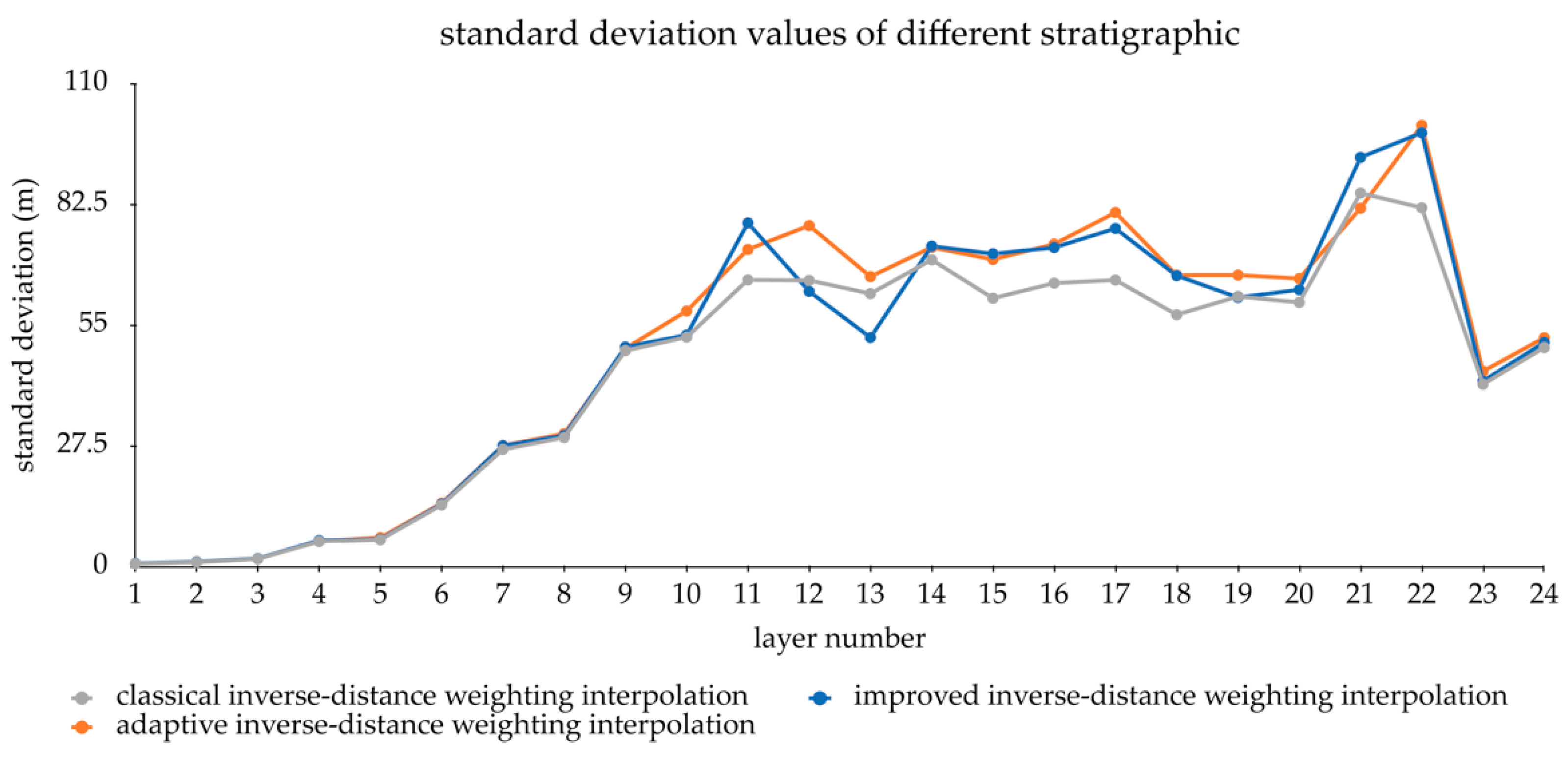
A comparison of the statistical indicators of the data sets (shown in Figure 13 and Figure 14) indicates that different interpolation methods have relatively consistent statistical indicator means and standard deviations, resulting in very similar interpolations.
The above analysis indicates that the data-adaptive inverse-distance weighting interpolation method proposed in this paper based on the first-order neighborhood selection strategy takes into account the spatial difference of geological attributes and can effectively improve the interpolation efficiency of large-scale geological modeling. In this case, compared with the existing improved inverse-distance interpolation algorithm, the adaptive inverse-distance interpolation can effectively reduce the computation time by 30%. When the shape of the local mass body becomes more complex, the proposed improved inverse-distance weighting interpolation method exhibits a better adaptability while generally maintaining the accuracy level of the existing inverse-distance interpolation method. Compared with the existing improved inverse-distance interpolation, adaptive inverse-distance interpolation only loses 7% accuracy. The testing shows that the adaptive inverse-distance interpolation algorithm proposed in this paper is efficient and stable and has high value. It can quickly generate large-scale geological models for application in practice. The proposed method can be used as a high-precision, high-reliability, and high-efficiency interpolation method for large-scale geological modeling of intelligent geology.
4. Conclusions
This paper proposes a data-adaptive inverse-distance weighting interpolation method based on the first-order neighborhood selection strategy, with the principles of classical inverse-distance interpolation, spatial differentiation of geological attribute data, and adaptability to geological attribute data characteristics. This method is mainly used to solve the accuracy, reliability, and validity problems of the inverse-distance interpolation algorithm in large-scale geological modeling.
Compared with the classical inverse-distance weighting interpolation method, the proposed method has better performance in efficiency and reliability. Compared with the improved inverse-distance weighting interpolation method, the proposed method has achieved a significant efficiency improvement under the condition of acceptable accuracy loss. In other words, the method proposed in this paper can simultaneously ensure the accuracy, reliability, and efficiency in the large-scale geological modeling process.
This method was applied to create a 3D geological model under an area in eastern China. The adaptive inverse-distance weighting interpolation method has a considerably better efficiency and can meet the accuracy, reliability, and efficiency demands for various geological models in the paper’s case. The actual test results show that the proposed method has high feasibility and reliability in actual applications, although there is an acceptable accuracy lost, which is acceptable to exchange for higher efficiency.
In this paper, we discussed the three inverse-distance weighting interpolation methods including classical, improved and adaptive inverse-distance weighting interpolation method. When the fluctuation of the geology body in the study area is small, and with no complex geology conditions, the classical inverse-distance weighting interpolation method is recommended; When the accuracy of the model is most important than any other factors such as efficiency, the improved inverse-distance weighting interpolation method is recommended. When the geology modeling requires efficiency, accuracy, and reliability, and the efficiency’s improvements is more important than small accuracy improvements, especially under the condition of complex geology body and big data, the adaptive inverse-distance weighting interpolation method is recommended.
The proposed method is not only suitable for large-scale geological modeling, but also can be applied to data-intensive computing tasks. It can provide efficient, reliable, and stable spatial interpolation for rain area model research, geospatial data visualization analysis, resource exploration, resource evaluation, geological mapping, and other fields.
Author Contributions
Conceptualization, Z.L. and C.Z.; Data curation, Z.Z.; Formal analysis, Z.Z. and W.M.; Funding acquisition, C.Z.; Methodology, Z.Z.; Project administration, Z.L.; Software, Z.Z.; Supervision, C.Z.; Validation, Z.L. and Z.Z.; Visualization, Z.D.; Writing–original draft, Z.Z.; Writing–review & editing, Z.L. All authors have read and agreed to the published version of the manuscript.
Funding
This research was funded by National Key Research and Development Program of China, grant number (2017YFC0804605,2017YFC1501203, 2017YFC1501201), the National Natural Science Foundation of China (NSFC) (Grant No. 41530638, 41977230), Key Project of Applied Science & Technology Research and Development of Guangdong Province, China (Grant no. 2016B010124007), Science and Technology Youth Top-Notch Talent Project of Guangdong Special Support Program (Grant no. 2015TQ01Z344) and Guangzhou Science and Technology Project (Grant no. 201803030005). The authors would like to thank the anonymous reviewers for their very constructive and helpful comments.
Institutional Review Board Statement
Not applicable.
Informed Consent Statement
Not applicable.
Data Availability Statement
Restrictions apply to the availability of these data. Data was obtained from Geological Survey of Jiangsu Province and are available at http://www.jsgs.com.cn with the permission of Geological Survey of Jiangsu Province.
Acknowledgments
The authors would like to thank the anonymous reviewers for their very constructive and helpful comments.
Conflicts of Interest
The authors wish to confirm that there are no known conflicts of interest associated with this publication and there has been no significant financial support for this work that could have influenced its outcome.
References
- Dorninger, P.; Nothegger, C.; Djuricic, A.; Rasztovits, S.; Harzhauser, M. Smart-Geology for the World’s Largest Fossil Oyster Reef. In Proceedings of the EGU General Assembly Conference Abstracts; 2014; p. 10504. Available online: https://ui.adsabs.harvard.edu/abs/2014EGUGA..1610504D/abstract (accessed on 8 December 2020).
- Zhou, C.; Du, Z.; Gao, L.; Ming, W.; Ouyang, J.; Wang, X.; Zhang, Z.; Liu, Z. Key technologies of a large-scale urban geological information management system based on a browser/server structure. IEEE Access 2019, 7, 135582–135594. [Google Scholar] [CrossRef]
- Rus, G.-M.; Dulama, M.E.; Ursu, C.-D.; Colcer, A.-M.; Ilovan, O.-R.; Jucu, I.S.; Horvath, C. Online Apps, Web Sources and Electronic Devices: Learning through Discovery about Valea Ierii Iara Valley. In Proceedings of the 14th International Conference on Virtual Learning, Bucharest, Romania, 25–26 October 2019; pp. 110–119. [Google Scholar]
- Mei, G. Summary on several key techniques in 3D geological modeling. Sci. World J. 2014, 2014, 1–11. [Google Scholar] [CrossRef] [PubMed]
- Qiao, P.; Lei, M.; Yang, S.; Yang, J.; Guo, G.; Zhou, X. Comparing ordinary kriging and inverse distance weighting for soil as pollution in Beijing. Environ. Sci. Pollut. Res. 2018, 25, 15597–15608. [Google Scholar] [CrossRef] [PubMed]
- Wojciech, M. Kriging method optimization for the process of DTM creation based on huge data sets obtained from MBESs. Geosciences 2018, 8, 433. [Google Scholar] [CrossRef] [Green Version]
- Mallet, J.-L. Discrete smooth interpolation in geometric modelling. Comput. Des. 1992, 24, 178–191. [Google Scholar] [CrossRef]
- Wang, Y.; Akeju, O.V.; Zhao, T. Interpolation of spatially varying but sparsely measured geo-data: A comparative study. Eng. Geol. 2017, 231, 200–217. [Google Scholar] [CrossRef]
- Shepard, D. A two-dimensional interpolation function for irregularly-spaced data. In Proceedings of the 1968 23rd ACM National Conference, New York, NY, USA, 27–29 August 1968; pp. 517–524. [Google Scholar]
- Varatharajan, R.; Manogaran, G.; Priyan, M.K.; Balaş, V.E.; Barna, C. Visual analysis of geospatial habitat suitability model based on inverse distance weighting with paired comparison analysis. Multimed. Tools Appl. 2018, 77, 17573–17593. [Google Scholar] [CrossRef]
- Chen, F.W.; Liu, C.W. Estimation of the spatial rainfall distribution using inverse distance weighting (IDW) in the middle of Taiwan. Paddy Water Environ. 2012, 10, 209–222. [Google Scholar] [CrossRef]
- Ilker, A.; Terzi, Ö.; Şener, E. Yağışın Alansal Dağılımının Haritalandırılmasında Enterpolasyon Yöntemlerinin Karşılaştırılması: Akdeniz Bölgesi Örneği. Tek. Dergi 2019, 540, 9213–9219. [Google Scholar] [CrossRef]
- Ahrens, B. Distance in spatial interpolation of daily rain gauge data. Hydrol. Earth Syst. Sci. 2006, 10, 197–208. [Google Scholar] [CrossRef] [Green Version]
- Wang, G.; Huang, L. 3D geological modeling for mineral resource assessment of the Tongshan Cu deposit, Heilongjiang Province, China. Geosci. Front. 2012, 3, 483–491. [Google Scholar] [CrossRef] [Green Version]
- Li, Z.; Li, X.; Li, C.; Cao, Z. Improvement on inverse distance weighted interpolation for ore reserve estimation. In Proceedings of the 7th International Conference on Fuzzy Systems and Knowledge Discovery, Yantai, Shandong, China, 10–12 August 2010; Volume 4, pp. 1703–1706. [Google Scholar]
- Blewitt, G.; Coolbaugh, M.F.; Sawatzky, D.L.; Holt, W.; Davis, J.L.; Bennett, R.A. Targeting of potential geothermal resources in the Great Basin from regional to basin-scale relationships between geodetic strain and geological structures. Trans. Geotherm. Resour. Counc. 2003, 27, 3–7. [Google Scholar]
- Tabatabaei, S.H.; Salamat, A.S.; Ghalandasrzadeh, A.; Riahi, M.A.; Beitollahi, A.; Talebian, M. Preparation of engineering geological maps of Bam City using geophysical and geotechnical approach. J. Earthq. Eng. 2010, 14, 559–577. [Google Scholar] [CrossRef]
- Liu, H.; Chen, S.; Hou, M.; He, L. Improved inverse distance weighting method application considering spatial autocorrelation in 3D geological modeling. Earth Sci. Inform. 2020, 13, 619–632. [Google Scholar] [CrossRef]
- Zalakeviciute, R.; Bastidas, M.; Buenaño, A.; Rybarczyk, Y. A Traffic-based method to predict and map urban air quality. Appl. Sci. 2020, 10, 1–18. [Google Scholar] [CrossRef] [Green Version]
- Malvić, T.; Ivšinović, J.; Velić, J.; Rajić, R. Interpolation of small datasets in the sandstone hydrocarbon reservoirs, case study of the sava depression, Croatia. Geoscience 2019, 9, 201. [Google Scholar] [CrossRef] [Green Version]
- Babak, O.; Deutsch, C.V. Statistical approach to inverse distance interpolation. Stoch. Environ. Res. Risk Assess. 2009, 23, 543–553. [Google Scholar] [CrossRef]
- Barbulescu, A.; Bautu, A.; Bautu, E. Optimizing inverse distance weighting with particle swarm optimization. Appl. Sci. 2020, 10, 2054. [Google Scholar] [CrossRef] [Green Version]
- Lu, G.Y.; Wong, D.W. An adaptive inverse-distance weighting spatial interpolation technique. Comput. Geosci. 2008, 34, 1044–1055. [Google Scholar] [CrossRef]
- Li, Z.; Zhang, X.; Zhu, R.; Zhang, Z.; Weng, Z. Integrating data-to-data correlation into inverse distance weighting. Comput. Geosci. 2020, 24, 203–216. [Google Scholar] [CrossRef]
- Ozelkan, E.; Bagis, S.; Ozelkan, E.C.; Ustundag, B.B.; Yucel, M.; Ormeci, C. Spatial interpolation of climatic variables using land surface temperature and modified inverse distance weighting. Int. J. Remote Sens. 2015, 36, 1000–1025. [Google Scholar] [CrossRef]
- Roberts, E.A.; Sheley, R.L.; Lawrence, R.L. Using sampling and inverse distance weighted modeling for mapping invasive plants. West. N. Am. Nat. 2004, 64, 312–323. [Google Scholar] [CrossRef]
- Jing, L.; Stephansson, O. Explicit Discrete Element Method for Block Systems—The Distinct Element Method. Dev. Geotech. Eng. 2007, 85, 235–316. [Google Scholar] [CrossRef]
- Sun, L.; Wei, Y.; Cai, H.; Yan, J.; Xiao, J. Improved Fast Adaptive IDW Interpolation Algorithm based on the Borehole Data Sample Characteristic and Its Application. J. Phys. Conf. Ser. 2019, 1284, 22–24. [Google Scholar] [CrossRef] [Green Version]
Figure 1.
Delaunay triangulation diagram. (a) Discrete data points; (b) Delaunay triangulation.
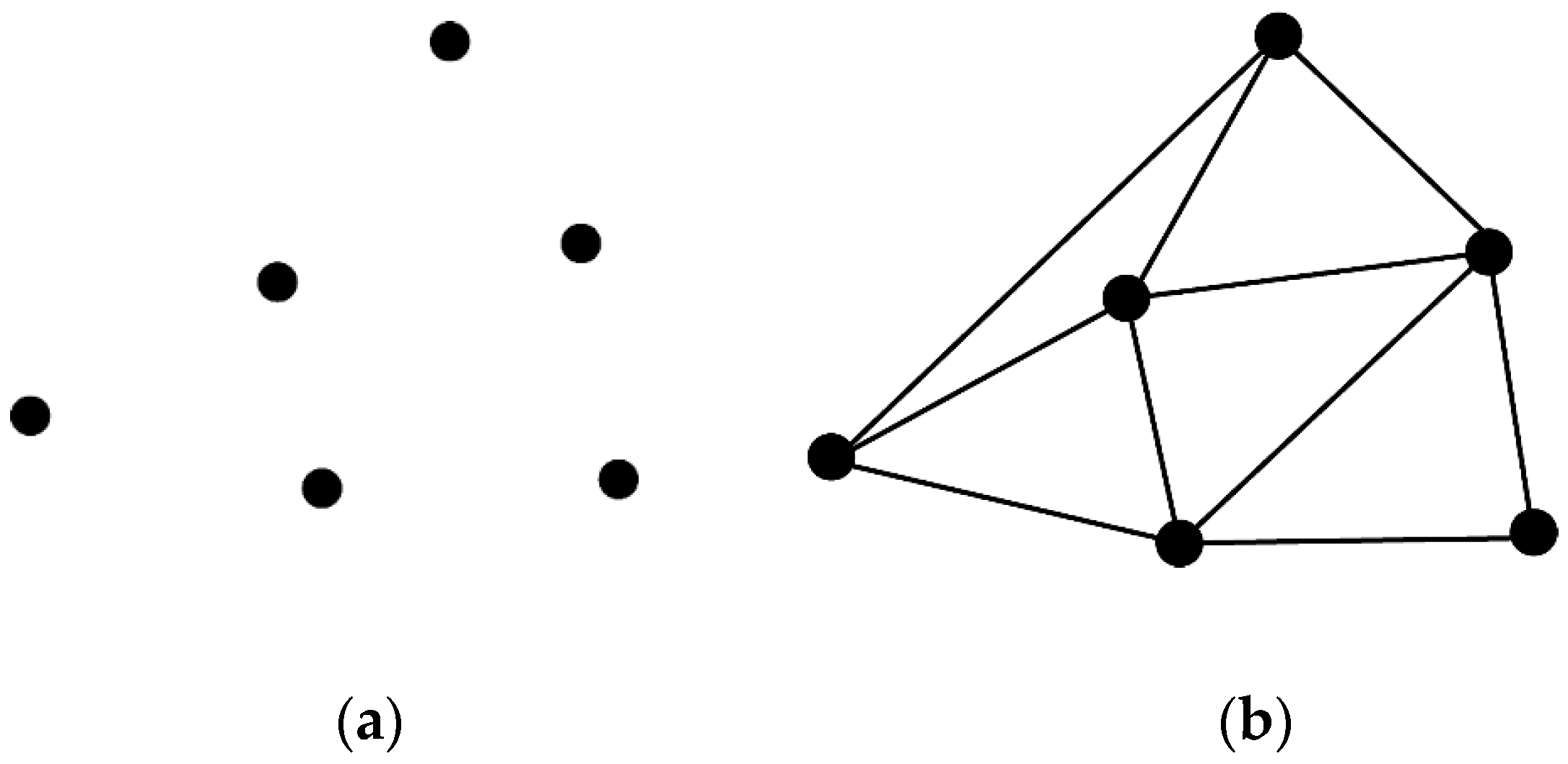
Figure 2.
Algorithm flow.
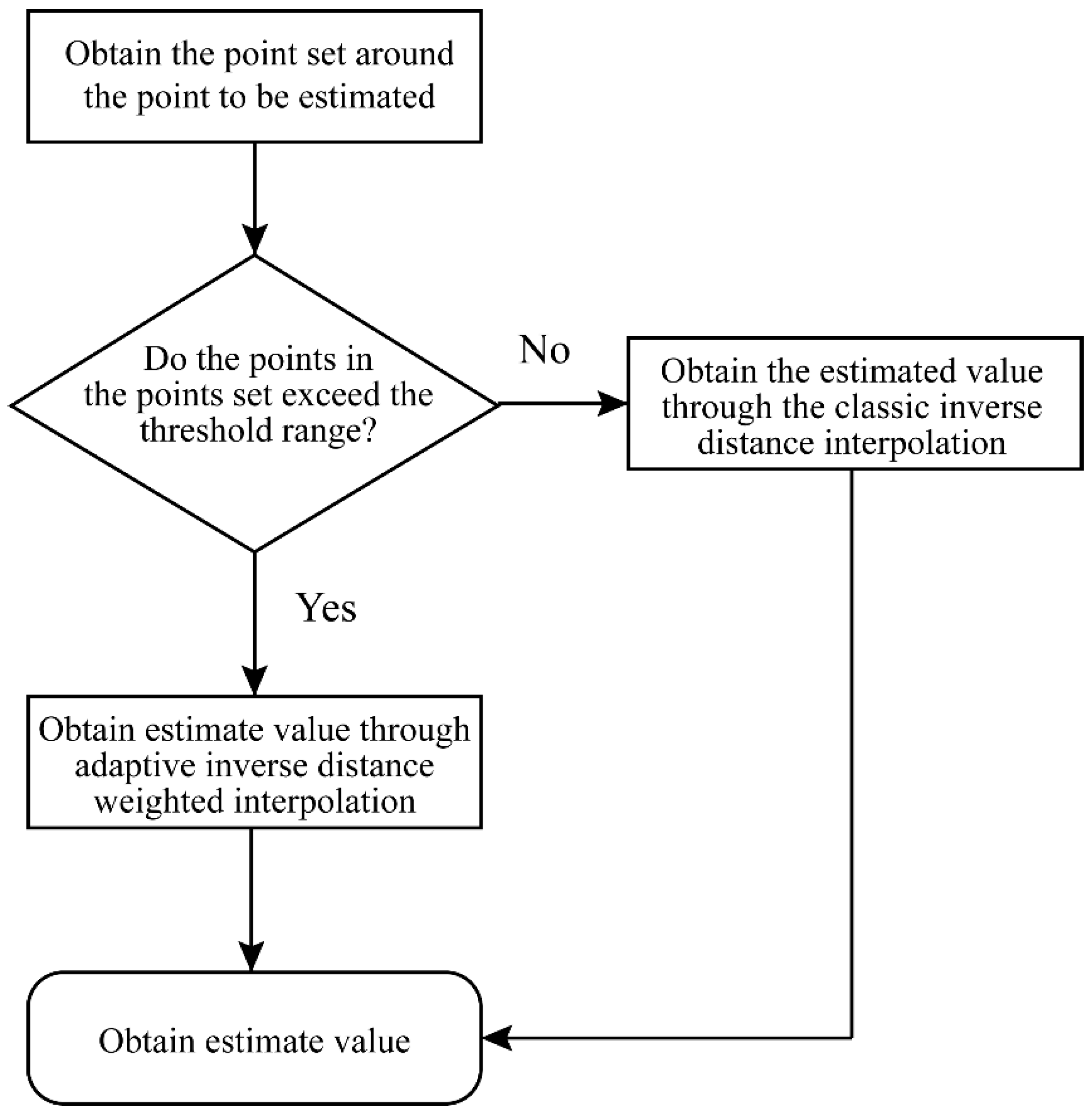
Figure 3.
Overview of borehole distribution.

Figure 4.
Schematic of different degrees of division. (a) First division; (b) second division; (c) third division.
Figure 4.
Schematic of different degrees of division. (a) First division; (b) second division; (c) third division.
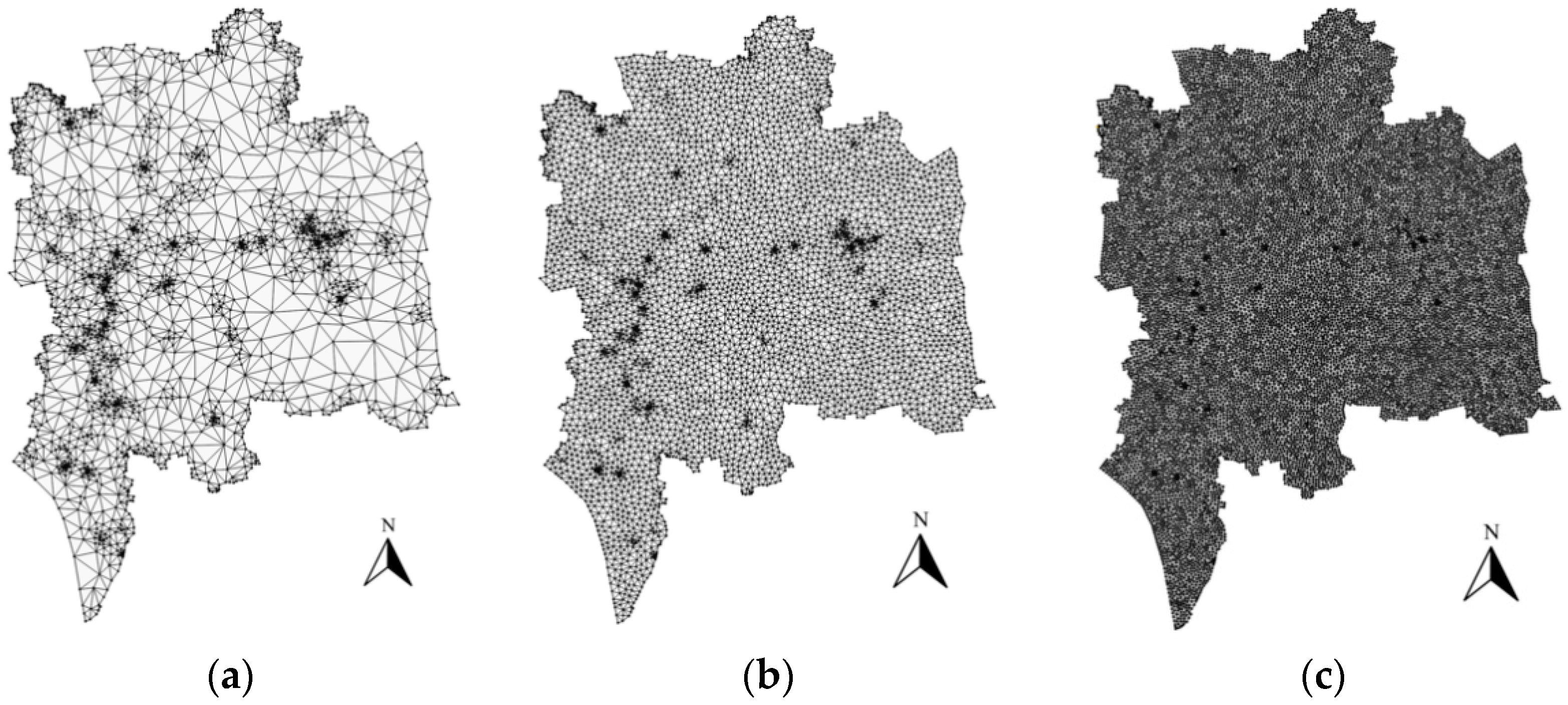
Figure 5.
Vertex numbers in different length bound.
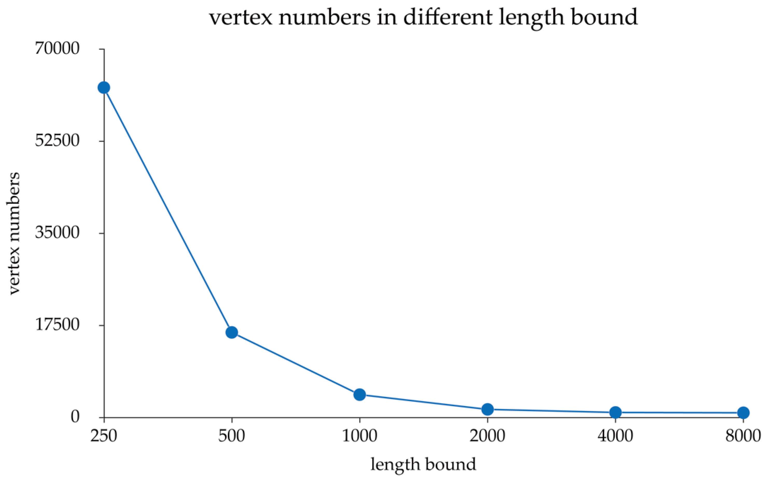
Figure 6.
Interpolated drilling display diagram.
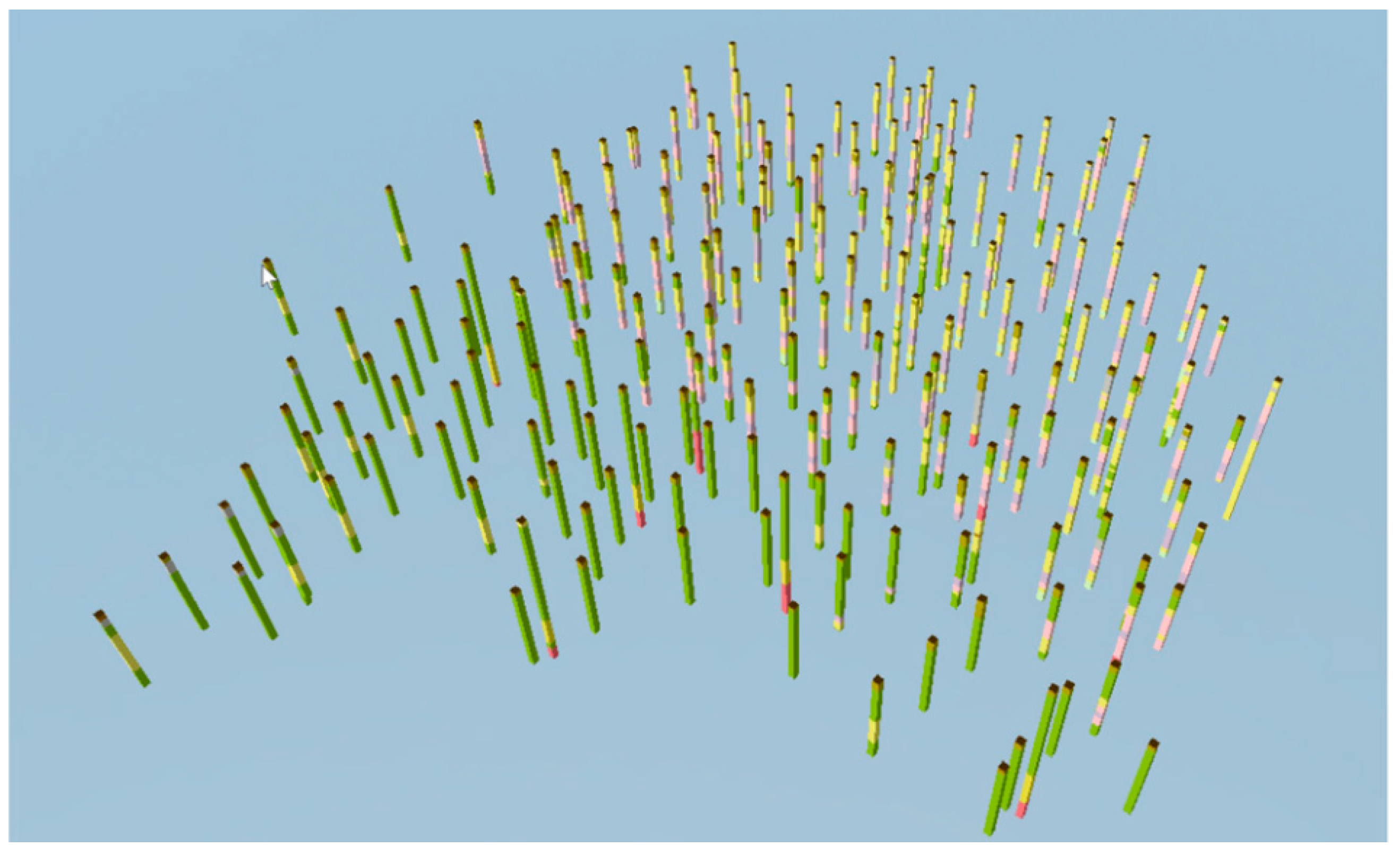
Figure 7.
Model renderings. (a) Overall angle of the geological model; (b) side orientation of the geological model; (c) separated geological units’ layers.
Figure 7.
Model renderings. (a) Overall angle of the geological model; (b) side orientation of the geological model; (c) separated geological units’ layers.
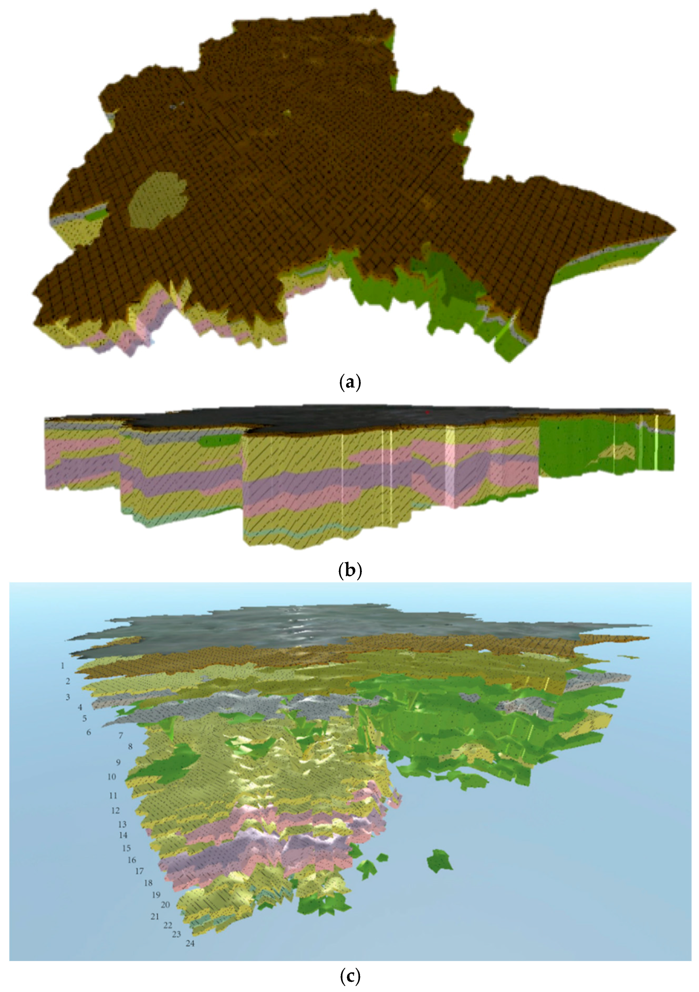
Figure 8.
The position of the profile.

Figure 9.
Interpolation viewpoint along the profile.
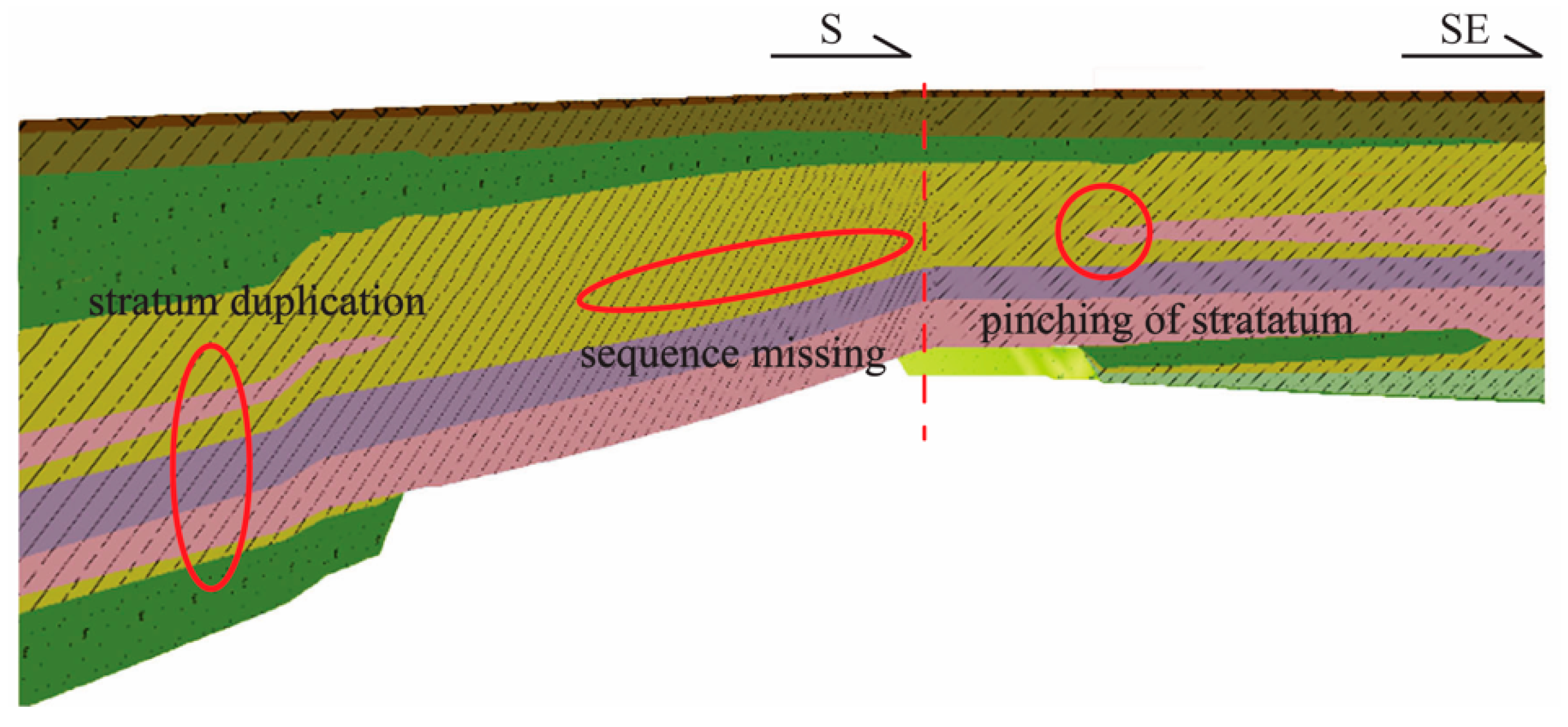
Figure 10.
Accumulative percentage error of different interpolation methods.
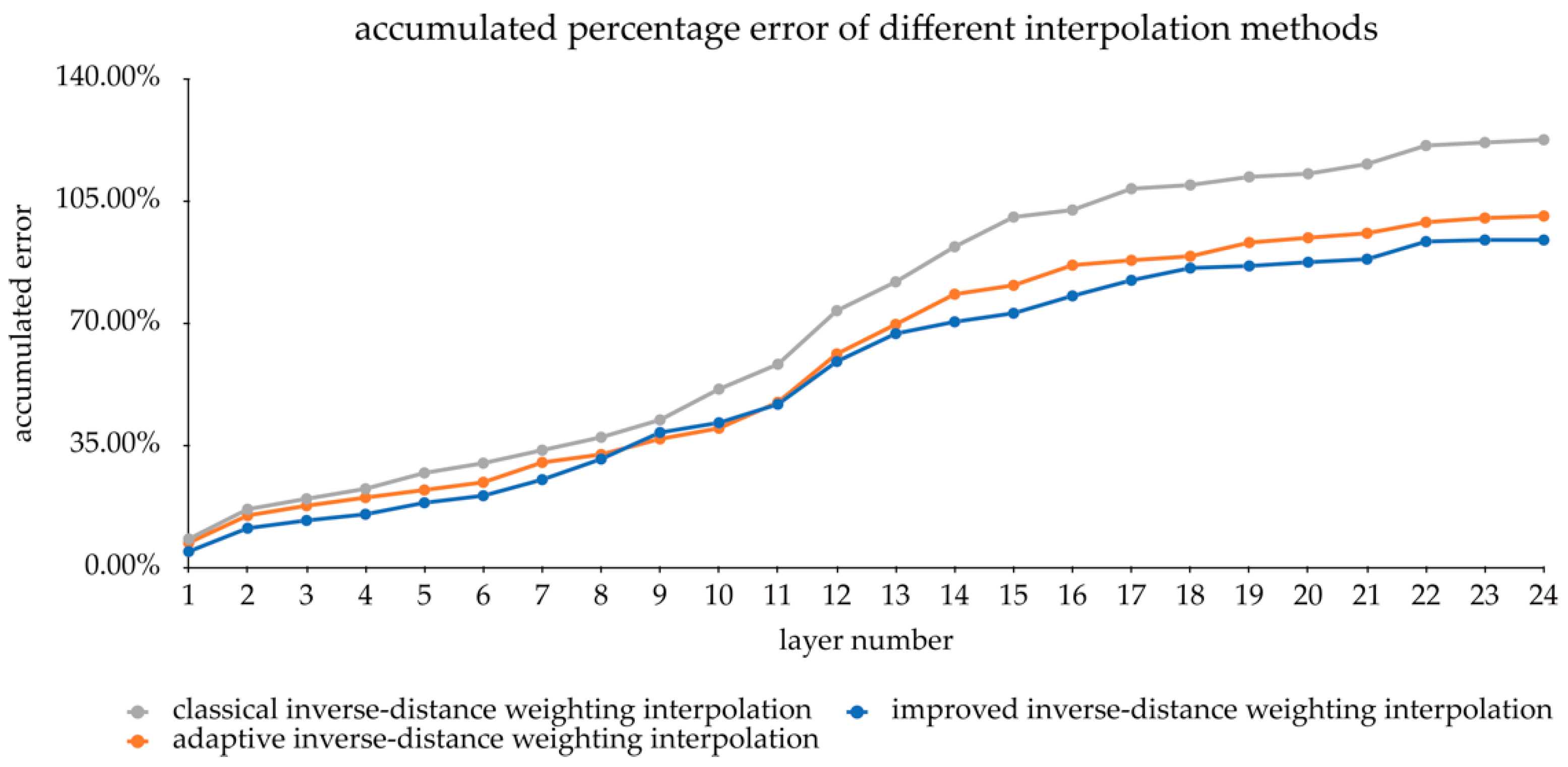
Figure 11.
Accumulated time consumption of different interpolation methods.

Figure 12.
Accumulated efficiency-error ratio of different interpolation methods.

Figure 13.
Mean values of different stratigraphic properties.
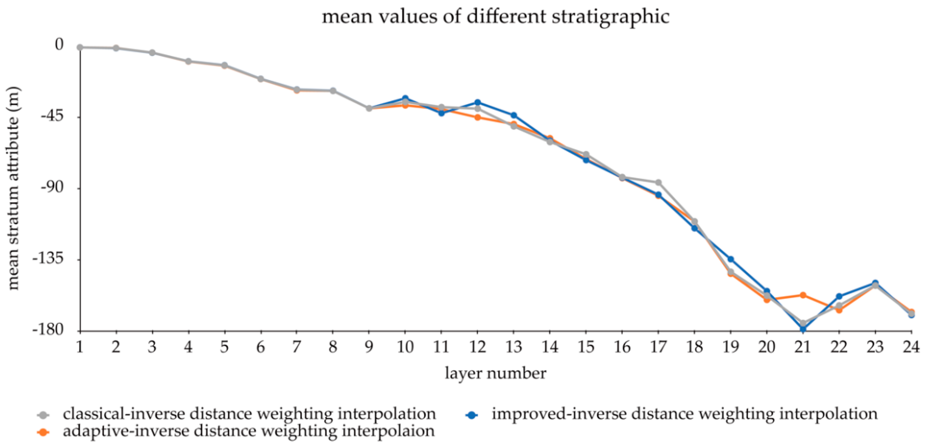
Figure 14.
Standard deviation of different stratigraphic properties.

Table 1.
Study area stratigraphic information.
| Age | Layer Number | Sublayer Number | Layer Name | Distribution | Property |
|---|---|---|---|---|---|
| Holocene | 1 | 1 | fill soil | Universal distribution | Plain fill, miscellaneous fill, flush fill, etc. |
| 2 | 2–1 | silty clay | Universal distribution | Greyish yellow to grey, slightly wet to saturated, waxy to soft plastic | |
| 2–2 | silt | Universal distribution | Greyish yellow to grey, wet to saturated, loose to slightly dense | ||
| 2–3 | siltstone | Universal distribution | Grey, saturated, partially silty sand, slightly dense to moderately dense, with developed horizontal bedding | ||
| 2-4 | muddy silty clay | Local region | Grey to grey-brown, flowing plastic, high moisture content, high compressibility | ||
| 2–5 | siltstone | Yangtze River alluvial plain | Grey to blue-grey, partially mixed with silt or including thin layers of silty clay, water-saturated, medium to dense | ||
| 2–6 | siltstone | Yangtze River alluvial plain | Grey to blue-grey, thin layer of silty soil or silty clay, water-saturated, moderately dense to dense | ||
| 2–6b | silty clay | Yangtze River alluvial plain | Grey to taupe, saturated, flowing plastic, thin layer of silt with silt soil, well-developed bedding | ||
| 2–7 | siltstone | Yangtze River alluvial plain | Grey to blue-grey, water-saturated, moderately dense to dense, well-developed bedding, with thin layer of silty clay partially intercalated | ||
| Late Pleistocene | 3 | 3–1 | siltstone(fine sand) | Yangtze River alluvial plain | Grey to grey-yellow, water-saturated, moderately dense to dense, with thin layers of cohesive soil in some areas, with well-developed bedding |
| 3–2 | fine sand(medium and coarse sand) | Yangtze River alluvial plain | Grey to grey-yellow, water-saturated, compact, lithology is fine gravel sand, with medium- to coarse-grained gravel sand, gravel layers, etc. | ||
| 4 | 4–1 | silty clay | Lixiahe plain | Grey-yellow to dark green, saturated, plastic to soft plastic, iron-manganese nodules, medium compressibility | |
| 4–2 | silty clay | Lixiahe plain | Grey-yellow to brown-yellow, dark green, iron-manganese nodules and calcium nodules, saturated, hard plastic to plastic, medium-low compressibility | ||
| 4–3 | silty clay mixed with silt | Lixiahe plain | Grayish yellow to grey, mixed with silt, saturated, plastic, moderate compressibility, horizontal bedding is relatively developed | ||
| 5 | 5–1 | silt, siltstone | Lixiahe plain | Mainly grey, grey-yellow in some areas | |
| 5–2 | silty clay | Lixiahe plain | Grey, saturated, soft-flow plastic, horizontal bedding development | ||
| 5–3 | siltstone | Lixiahe plain | Grey, saturated, moderately dense to dense | ||
| 6 | 6 | cay, silty clay | Lixiahe plain | Lacustrine sediments, distributed in the Lixiahe plain | |
| 7 | 7–1 | silt, siltstone | Lixiahe plain | Greyish yellow, blue-grey, water-saturated, moderately dense to dense, well-layered | |
| 7–2 | silty clay | Lixiahe plain | Greyish yellow, blue-grey, saturated, plastic-soft plastic, bedding is relatively developed | ||
| Middle Pleistocene | 8 | 8–1 | siltstone, fine sand | Yangtze River alluvial plain | Grey, greyish yellow, part of the area is medium sand, partly with gravel and dense |
| 8–2 | gravel sand (gravel layer) | Yangtze River alluvial plain | Mainly grey, partially greyish yellow, with large lithological changes | ||
| 9 | 9–1 | silty clay | Lixiahe plain | Cyan-grey to grey-yellow, saturated, mainly hard plastic but can also be partially plastic, containing iron-manganese nodules and calcium nodules | |
| 9–2 | silty clay with silt | Lixiahe plain | Greyish yellow grey, saturated, plastic-soft plastic, high silt content, well-developed layering | ||
| 9–3 | silty clay | Lixiahe plain | Cyan-grey to yellow, saturated, hard plastic to partially plastic |
Table 2.
The efficiency-error ratio of different interpolation methods and stratum numbers.
| Strata Number | Classical | Adaptive |
|---|---|---|
| 1 | 0.04 | 0.02 |
| 2 | 0.23 | 0.02 |
| 3 | 0.83 | 0.43 |
| 4 | 1.58 | 1.05 |
| 5 | 2.45 | 2.20 |
| 6 | 3.40 | 3.54 |
| 7 | 4.73 | 4.89 |
| 8 | 7.02 | 11.47 |
| 9 | 11.52 | 17.45 |
| 10 | 13.10 | 24.27 |
| 11 | 14.57 | 44.03 |
| 12 | 15.84 | 49.95 |
| 13 | 17.35 | 55.73 |
| 14 | 18.51 | 57.84 |
| 15 | 19.47 | 60.08 |
| 16 | 20.67 | 62.32 |
| 17 | 21.85 | 65.76 |
| 18 | 23.18 | 71.56 |
| 19 | 24.47 | 74.58 |
| 20 | 25.82 | 77.59 |
| 21 | 27.07 | 80.60 |
| 22 | 28.37 | 85.04 |
| 23 | 29.68 | 89.03 |
| 24 | 30.98 | 92.74 |
Publisher’s Note: MDPI stays neutral with regard to jurisdictional claims in published maps and institutional affiliations. |
© 2021 by the authors. Licensee MDPI, Basel, Switzerland. This article is an open access article distributed under the terms and conditions of the Creative Commons Attribution (CC BY) license (http://creativecommons.org/licenses/by/4.0/).
Share and Cite
MDPI and ACS Style
Liu, Z.; Zhang, Z.; Zhou, C.; Ming, W.; Du, Z. An Adaptive Inverse-Distance Weighting Interpolation Method Considering Spatial Differentiation in 3D Geological Modeling. Geosciences 2021, 11, 51. https://doi.org/10.3390/geosciences11020051
AMA Style
Liu Z, Zhang Z, Zhou C, Ming W, Du Z. An Adaptive Inverse-Distance Weighting Interpolation Method Considering Spatial Differentiation in 3D Geological Modeling. Geosciences. 2021; 11(2):51. https://doi.org/10.3390/geosciences11020051
Chicago/Turabian StyleLiu, Zhen, Zhilong Zhang, Cuiying Zhou, Weihua Ming, and Zichun Du. 2021. "An Adaptive Inverse-Distance Weighting Interpolation Method Considering Spatial Differentiation in 3D Geological Modeling" Geosciences 11, no. 2: 51. https://doi.org/10.3390/geosciences11020051
Note that from the first issue of 2016, this journal uses article numbers instead of page numbers. See further details here.