Abstract
In this paper, object-based image analysis classification methods are developed that do not rely on backscatter in order to classify the seafloor. Instead, these methods make use of bathymetry, bathymetric derivatives, and grab samples for classification. The classification is performed on image object statistics. One of the methods utilizes only texture-based features, that is, features that are related to the spatial arrangement of image characteristics. The second method is similar, but relies on a wider set of image object features. The methods were developed and tested using a dataset from Norwegian waters, specifically the Røstbanken area off the coast of Lofoten. The classification results were compared to backscatter-based classification and to grab sample ground-reference data. The algorithm that performed the best was then also applied to a dataset from the Borkumer Stones area close to the island of Schiermonnikoog in Dutch waters. This allowed testing the applicability of the algorithm for different datasets. Because the algorithms that were developed do not require backscatter, the availability of which is much more scarce than bathymetry, and because of the low computational requirements, they could be applied to any area where high-resolution bathymetry and grab samples are available.
1. Introduction
Seafloor mapping has a long history with merchants in the Mediterranean making some of the first organized efforts [1]. Further development of bathymetric maps has continued to the present day [2]. Modern seafloor mapping extends beyond bathymetry and also includes backscatter, a co-located product delivered by multibeam echosounder (MBES) sonars. Backscatter is increasingly used to characterize or classify the seafloor [3,4,5,6,7,8,9]. Classification methods range widely, including the use of neural networks [10,11,12], principle component analysis (PCA) [6,13,14,15,16,17], Bayesian decision rules [4,5,6,8,18,19], and textural analysis [20], among others. A recent development to further increase the use of backscatter is the capability of some MBES systems to deliver multi-spectral backscatter data [21] in a single pass over an area of seafloor [8,9]. Currently, only R2Sonic MBES systems [22] have this capability. Despite backscatter being the preferred datatype for seafloor classification, it remains less available than bathymetry data [23]. Due to the need for up-to-date navigational charts, large portions of the coastal seas are already mapped with high-resolution bathymetry [24]. For the Dutch Continental Shelf (DCS), and the rest of European waters, full coverage bathymetry data, albeit at lower resolution, are also available for download via the European Marine Observation and Data Network (EMODNet) [25]. Although some backscatter data were made available by the Rijksdienst voor Ondernemend Nederland (RVO) for the De Rijke Noordzee project [26], a centralized backscatter data repository is not in place. At the global scale, less than 18% of the oceans have been directly measured by echosounders [27]. These efforts focus on bathymetry without the mention of backscatter. It would, therefore, be desirable to develop a fast and robust classification method that uses bathymetry and bathymetric derivative layers as input instead of backscatter.
An approach to use the more available bathymetry data, rather than backscatter, for a classification algorithm is an object-based image analysis (OBIA)-based method [28]. OBIA has been widely used for terrestrial mapping [29] and in the past few years has also been increasingly used for seafloor classification [28,30,31,32,33]. Le Bas [34] also developed an arcGIS add-on for OBIA analysis. A strength of the OBIA approach is that image objects can be formed at multiple layers, and the wide range of sub-object features can all be harnessed for classification purposes.
The goal of this paper is three-fold. The first goal is to develop an OBIA-based classification method that only uses bathymetry, bathymetric derivatives, and grab sample ground-reference data as input. Secondly, an approach that only uses texture image object features, that is, features that relate to the arrangement of image characteristics instead of the image values themselves, is implemented and tested. Finally, the best performing method is used to investigate how transferable it is to other geographical areas with minimal loss of classification accuracy and minimal adjustment of the algorithm. The developed methods are validated by comparing them to both backscatter-based classification and to grab sample ground-reference data. Finding a non-backscatter-based classification method would have significant implications for the use of legacy bathymetry data as well as the 2030 global coverage bathymetry [27] data for seafloor classification purposes.
2. Study Area, Materials, and Methods
2.1. Study Areas
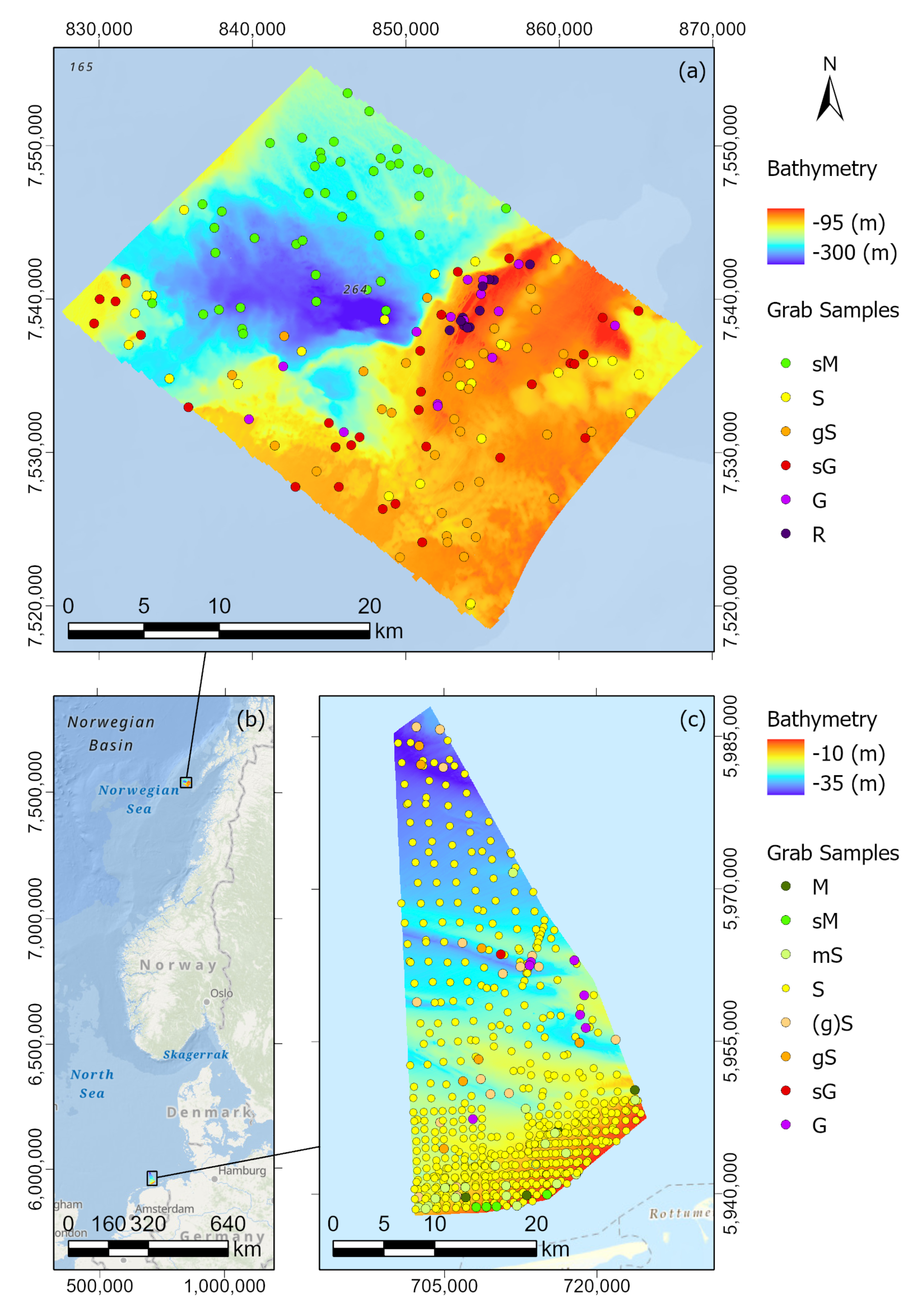
Datasets from two study areas are considered in this paper. The first of these study areas is in the Norwegian Sea, ~50 km off the coast of Lofoten, more specifically, off the coast of the Røst Islands (Figure 1a). For the remainder of the paper, this study area is referred to as the Røstbanken area. The dataset from the Røstbanken area includes both backscatter and bathymetry. The data were made available during the 2016 OBIA workshop of the GeoHab conference [35]. The second dataset is from the Borkumer Stones area of the Dutch North Sea (Figure 1c). This area is close to the border between Dutch and German waters and the dataset begins only ~10 km off the coast of the Dutch island of Schiermonnikoog, one of the Frisian Islands.
For the Røstbanken study area, both bathymetry and backscatter data are available for a rectangular area ~22 km wide and ~32 km long. The water depth ranges from just under 100 m to almost 300 m deep. The general Røstbanken area shows the typical architecture and glacial land forms that are produced by slow-flowing regions of an ice sheet [36]. During the last glacial maximum, slow moving ice is thought to have covered the Røstbanken area [37]. Røstbanken is also heavily scoured by linear to curvilinear depressions, likely produced by the keels of icebergs [36]. Several such plow marks are visible in the Røstbanken data. For the Røstbanken area, 157 grab samples are available, which indicate a very wide range of sediments from sandy mud to rock.
The water depth in the Borkumer Stones study area ranges in depth from 10 to 35 m (Figure 1c). A triangular area of data was made available by the Hydrographic Service of the Royal Netherlands Navy. In the south and north, the dataset is ~23 and ~5 km wide, respectively. In the south to north direction, the dataset is ~50 km long. Much of the seabed of the Borkumer Stones area consists of coarse sand [38], but stones and rocks have also been mapped in this area [39]. Through the years, the presence of reefs have also been found [38,39,40]. Coolen et al. [38] found areas of dense L. conchilega beds. For the Borkumer Stones area, 567 grab samples were used for ground truthing the classification results [41,42].
Figure 1.
(a) Bathymetry of the Røstbanken study area. Grab sample locations are shown and the symbols indicate the sediment type in Folk classes (R indicates rock). (b) The locations of the two study areas considered in this paper (data source: [43]). (c) Bathymetry of the Borkumer Stones study area. Grab sample locations are shown and the symbols indicate the sediment type in Folk classes.
2.1.1. The Base Geo-Tiff Images
All of the bathymetry and backscatter data for this study are in the form of geo-tiff data images gridded at a 5 m × 5 m resolution. The images were geo-referenced, that is, the exact geographic location of each pixel is known. The Røstbanken data and the Borkumer Stones data used the WGS 1984 UTM Zone 32N and ETRS 1989 UTM Zone 31N spatial reference systems, respectively. Although the data had several different coordinate systems, the results presented in this paper are all projected in the ETRS 1989 UTM Zone 31N spatial reference system for uniformity.
The Røstbanken bathymetry data were collected by multibeam echosounding. The exact location of the sonar, and by extension the location of seafloor being measured, is known based on GPS data combined with the use of MRU data. The bathymetry data were cleaned and are of high quality. The backscatter data were geo-referenced, and the angular dependence was removed as outlined in [44]. The backscatter was also corrected to compensate for differences in ensonified area and spreading.
For the Borkumer Stones area, only bathymetry, but not backscatter, was available. The northern part of the research area had some data gaps that were interpolated in ArcGIS prior to the layer being used for analysis. Some MBES lines, especially towards the south of the area, had motion artifacts. This was suspected because there were swath wide artifacts perpendicular to the sailing direction, a tell-tale sign of motion artifacts [45]. These types of artifacts can be corrected when raw MRU motion and MBES time of travel information is available [45]. Because the raw data were not available for this research, these artifacts were not removed. The effect of the artifacts on the classification performance is discussed in Section 4.3.
2.1.2. Bathymetric Derivative Layers
In addition to the base layers, which are bathymetry and backscatter, several bathymetric derivative layers were created. These included slope, curvature, aspect, and Bathymetric Position Index (BPI) layers.
Slope
The slope of the seafloor is calculated from the bathymetry with the values indicating the deviation from the horizontal in degrees. The slope is calculated with the built-in ArcGIS slope function from the 3D Analyst toolbox. The formula for the calculation of the slope s is as follows
where
and
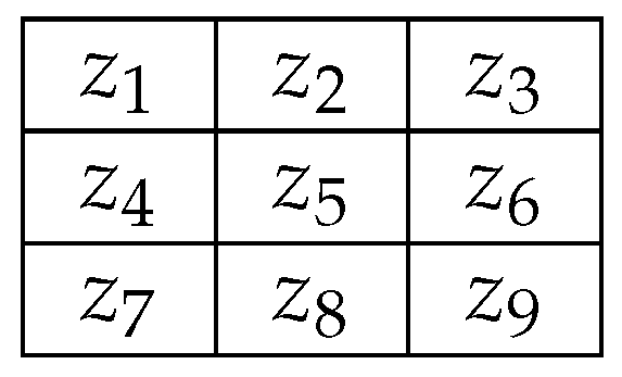
where and refer to the cell (or pixel) size in the x and y (or north and east) directions, respectively, and z is the depth, or pixel value, where subscripts 1–9 refer to the pixels surrounding the pixel with subscript 5 as in Figure 2, where the slope is being calculated for pixel .
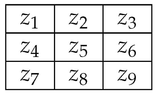
Figure 2.
Schematic of the pixels used for the calculation of the slope and curvature.
Smoothed Slope
Additionally, a slope-based layer was created, namely a smoothed slope. Each pixel in this layer is the mean of the pixels within a radius of 1 km. This layer has larger values for pixels closer to areas of high slopes, and especially to large areas of high slopes. Importantly, the values do not drop off just outside of a high slope area as the slope layer itself does.
Curvature
The curvature of the seafloor is the slope of the slope, or second derivative, of the seafloor and is created with the ArcGIS curvature function according to the method set forth in [46]. The curvature is calculated for point (Figure 2) by taking the depth values at points – as defined in Figure 2 and fitting a quadratic polynomial of the form
to these points. This 9-term polynomial exactly fits all 9 points in the moving grid. The curvature is the Laplacian of Equation (4) [47,48] and, because z can be defined such that is at , simplifies to
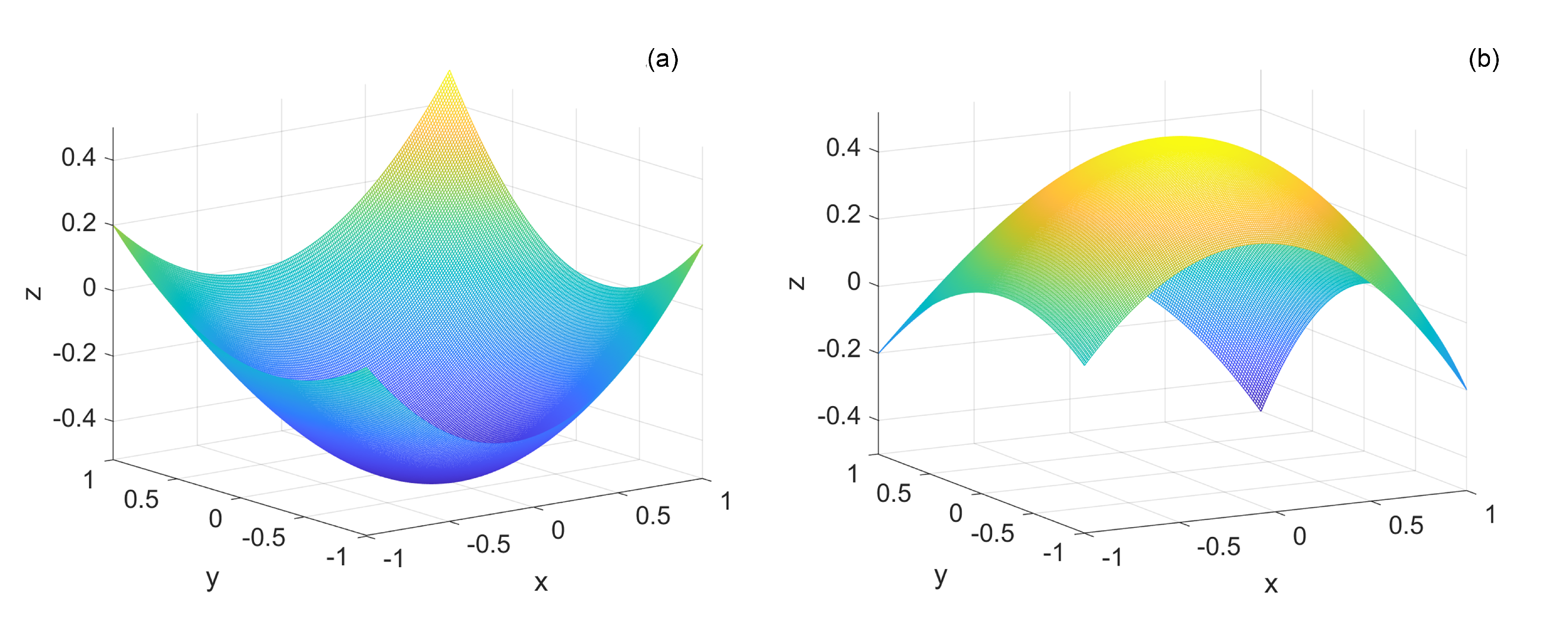
where , , and L is the pixel size ( for this application). In our implementation, is used for the actual resultant values in the curvature layer. Thus, a negative value indicates a convex-down seafloor (Figure 3a) and a positive value a convex-up seafloor (Figure 3b). A value of zero indicates an area where there is no curvature.
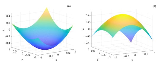
Figure 3.
(a) An example of a convex-down seafloor; and (b) an example of a convex-up seafloor.
Aspect
The aspect indicates the compass direction of the steepest slope, and is calculated with
where and are as defined in Equations (2) and (3). The aspect layer is created using the Aspect tool in the ArcGIS 3D Analysis toolbox. The aspect can fall between the values of 0 being true north and 360 again being north. A shortcoming of using aspect in some situations is that there is a discontinuity at due north. That is, a slope direction of north, northwest, will have values close to 360 and a similar slope direction of north, northeast, will have values close to 0.
Bathymetric Position Index
The Bathymetric Position Index (BPI) is the underwater equivalent of the terrestrial “Topographic Position Index” that is often used as a parameter for habitat modeling [49,50,51]. The BPI is a measure of seafloor depth relative to the surrounding seafloor and is defined as follows
where is the mean depth indicated by all pixels within a given radius of the pixel . Needless to say, the resulting BPI layer depends strongly on . With smaller , local features are accentuated, but, with large enough , regional features are dominant. Ten different BPI layers were created with and radius, in pixels and distance, respectively, shown in Table 1.

Table 1.
Radii in distances for BPI layers with radii measured in pixels .
2.2. Methods
All of the layers described in the previous section are used in a segmentation algorithm to create image objects. Statistics from the image objects are then used for seafloor classification. The creation of both the image objects and the classification methods is now addressed. The segmentation and classification is carried out using the Trimble software eCognition (versions 9.2.1 and 9.5.0).
2.2.1. Object-Based Image Analysis
Image Objects
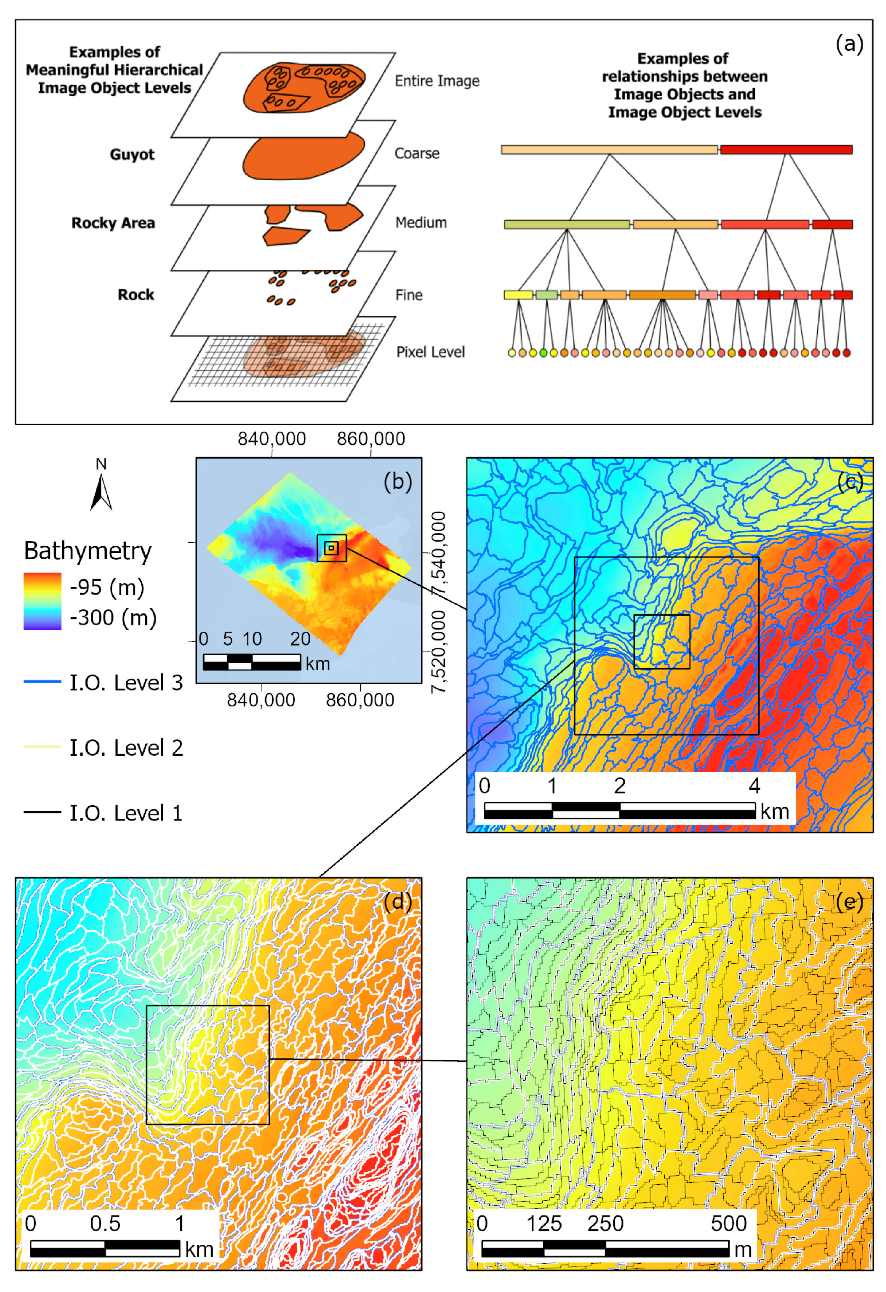
The principle for OBIA is that instead of considering an image only on the basis of its pixels, it is considered on the bases of image objects, where an image object is defined as a set of image pixels. Image objects are furthermore organized into different levels. At the pixel level the image objects are the same as the pixels (see Figure 4a). A segmentation of the image, starting from the pixel level, creates a higher level of image objects (this layer is called “Fine” in Figure 4a). Further segmentation can then be carried out on the image object level to create even higher levels of image objects (“Medium” and “Coarse” in Figure 4a).
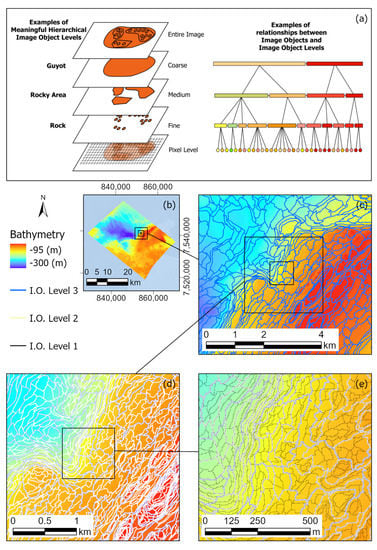
Figure 4.
(a) Examples of meaningful hierarchicalimage object levels and relationships between image objects and image object levels (sub-figure after [52,53]). (b) Bathymetry of the Røstbanken study area, where black rectangles indicate the extents depicted in (c–e). (c) Blue polygons indicate Level 3 (“Coarse” in (a)) image objects, the black rectangles indicate the extents of (d,e), and the background color indicates bathymetry (also holds for (d,e)). (d) White polygons indicate Level 2 (“Medium” in (a)) image objects, borders shared between image objects of Level 2 and 3 have a blue outline, and the black rectangle indicates the extent shown in (e). (e) Black polygons indicate Level 1 image objects (“Fine” in (a)), borders shared between image objects of Level 1 and 2 have a white outline, and borders shared between image objects of Level 1 and 3 have a blue outline.
For each of these image objects, a host of statistics can be calculated to create image object features. These features are later used during the classification stage. Image object features include statistics about the size, shape, or the mean color (color here, and for the rest of the manuscript, refers to the pixel value (or the mean value of sub-objects in the case of higher level segmentations) of a particular image) of any of the layers of an object. They can also include features of image objects at different levels. For example, to carry out a classification at image object Level 3 (Figure 4c), image object features of sub-objects at Level 2 (objects with white borders in Figure 4d) or at Level 1 (objects with black borders in Figure 4e) can be used. Finally, the use of features from neighboring image objects are also used in this paper.
Creating Image Objects by Multiresolution Segmentation
A very commonly used image segmentation algorithm in OBIA is the multiresolution segmentation algorithm [54]. This algorithm starts by considering every pixel within an image to be an image object. Neighboring image objects are iteratively merged to form larger image objects while minimizing the within object heterogeneity h [55]. The heterogeneity, as described by Benz et al. [53], is a combination of both color c and shape s heterogeneity. The heterogeneity change is defined as
where and are user specified weights such that and . These weights allow the value of the heterogeneity to be adapted for emphasis on color or shape heterogeneity. For example, a bathymetry layer might have the value of −32 that corresponds to the depth at that pixel location. The amount of color heterogeneity change is defined as
Here, N is the number of image layers considered in the segmentation process (see Table 2), is the weight assigned to the ℓth image layer, refers to the number of pixels in the image object, and is the within object standard deviation of image object i of image layer ℓ. The subscript refers to the separate objects 1 and 2 that are being considered for merging or to the potential image object m that would result from merging image objects 1 and 2.

The shape s of an image object is dependent on the compactness and smoothness of an image object. Compactness is the ratio of the perimeter length of the image object and the area of the image object. Smoothness is the ratio of the perimeter length of the image object and the perimeter length of the bounding box within which the image object would fit [53]. The change in the shape heterogeneity is given by
where and are user specified and restricted as and are.
Compactness change is given as
where n is the number of pixels in the object and p is the perimeter of the image object. The subscripts and 2 refer to the merged object, object 1, and object 2, as defined above. The change in smoothness is given as
where b is the perimeter of a box that bounds the object and n, p, and the subscripts are defined as above.
For every loop of the algorithm, each image object is “visited” once [55] (p. 68). For a starting “seed” image object , the algorithm looks for the neighboring image object such that, if they were merged, the heterogeneity change would be minimum, i.e., the best fit. If the best fit for image objects and is not mutual, then object becomes the seed to continue the search for objects to merge. This process is stopped when no more image objects can be merged such that is less than a certain, user specified, threshold called a “scale parameter” .
For this research, three levels of segmentation were performed (Figure 4c–e) with different settings per segmentation level (Table 2). For the first of the image object levels, the finest level, the image objects were intended to conform to the smallest features in the bathymetry. To accomplish this, the generated image layers were examined to see which layers most clearly showed small-scale seabed features. Small scale features, as referred to in this work, are of such size that they are present over at least a few image pixels. They are the smallest distinct features that can be reliably perceived in the data by visual inspection. Because they span a few image pixels, they are likely to measure several tens of meters physically. Image layers that were useful at first level were layers such as slope, BPI layers with a small radii, and aspect. Although the aspect layer accentuates small features, it was not used, because of its discontinuity at due north. The image layer weights and the scale parameter were selected such that the shapes of the image objects conformed to the small-scale seafloor features. Additionally, the heterogeneity used during the segmentation process depended largely on color and not on image object shape (see Section 2.2.1). This allowed the shapes of the image objects to better conform to the shapes of small-scale seafloor features, which allowed shape related image object features (statistics) to better indicate the presence of seafloor features.
At the second level of image objects, it was still desired that image objects would conform to small seafloor features. However, to gain the most benefit from having multiple image object layers, it was necessary to select a scale parameter such that each image object at this level was composed of at least a few image objects from the lower level. As was the case for the segmentation at Level 1, the heterogeneity of the segmentation was set to mostly be dependent on the color parameter and not on the shape parameter.
At the third level of image object segmentation, the focus changed significantly. At this level, much more emphasis was placed on image object shape and less on image object color. In addition, the choice of layer(s) was made such that larger scale seafloor features would fall within image objects. Based on a subjective examining of the different layers, was a good layer to use for this segmentation level. The larger the image objects were, the more lower level sub-objects they contained. Because the texture-based features were calculated from sub-objects, larger image objects and more sub-objects also meant that the discrimination power of texture features was greater. However, because making the image objects too large would decrease the resolution of the classification results, a balance in image object size was sought. In any case, the scale parameter was selected such that multiple image objects of Levels 1 and 2 were contained in image objects at Level 3.
2.2.2. Classification
Three methods of classification are used in this paper. Each of the methods is performed on image objects features which were discussed in the previous section. The three classification methods are as follows:
- Method 1 is threshold based and uses image object features from the backscatter, bathymetry, and layers. The thresholds are those used in the 2016 OBIA workshop of the GeoHab conference [35] and were developed at the Center for Environment Fisheries and Aquaculture Science (CEFAS) [56]. This approach was not developed within the current research, but its results are considered as a standard to which Methods 2 and 3 can be measured.
- Method 2 uses a Classification And Regression Tree (CART), a binary tree predictive model to go from observations about an item to conclusions about the items target value or class (a more in-depth description follows below) [57]. The CART provides the thresholds which are then used in a similar way as in Method 1. This method uses only texture features from image objects.
- Method 3 is similar to Method 2, however, it uses both texture and direct layer image object features. That is, it does not only use texture-based features, which relate to the arrangement of layer values, but it also references layer values directly, such as the average depth within an image object.
The image objects at Level 3, created by the third application of the multiresolution segmentation, are used to classify the seafloor sediments. Grab samples classified according to Folk are used to create a training dataset for a classification and regression tree (CART). Firstly, each image object that coincides with the location of a grab sample is classified according to the Folk class of that grab sample. Based on these classified image objects the CART is constructed.
The CART is constructed in a top down greedy approach. At each step, an image object feature at Level 3 is chosen that best splits the set of classified image objects. The Gini impurity index is used to measure the “best” split. It is calculated for each candidate subset and the results are combined to form a measure of the quality of the split. The Gini impurity at node is calculated as
where is the fraction of items labeled as class i and where J is the number of classes. reaches its minimum () when all cases in a node are of the same class.
After the classification tree is constructed, every image object at Level 3 is classified using the tree. Given the attributes of the image object, the decision tree is traversed from the root node until it is classified at a leaf node (brightly colored rectangles in of the tree.
To compare the classification to grab sample ground-reference data, the grab sample sets were subdivided to create a training and a validation set. For the comparisons against other classification methods, the full grab sample set was used as a training set for the CART.
The final classification map was greatly improved by cleaning up the classification results as follows. For each research area, the most common seafloor sediment type was used such that any image object classified in a different class, but surrounded or largely surrounded by the sediment type that was most dominant, was reclassified into the most dominant class. For the Røstbanken data, this dominant class was sandy mud. For the Borkumer Stones area, this class was sand. Making use of a clean up step similar to this is common practice in OBIA classification algorithms.
3. Results
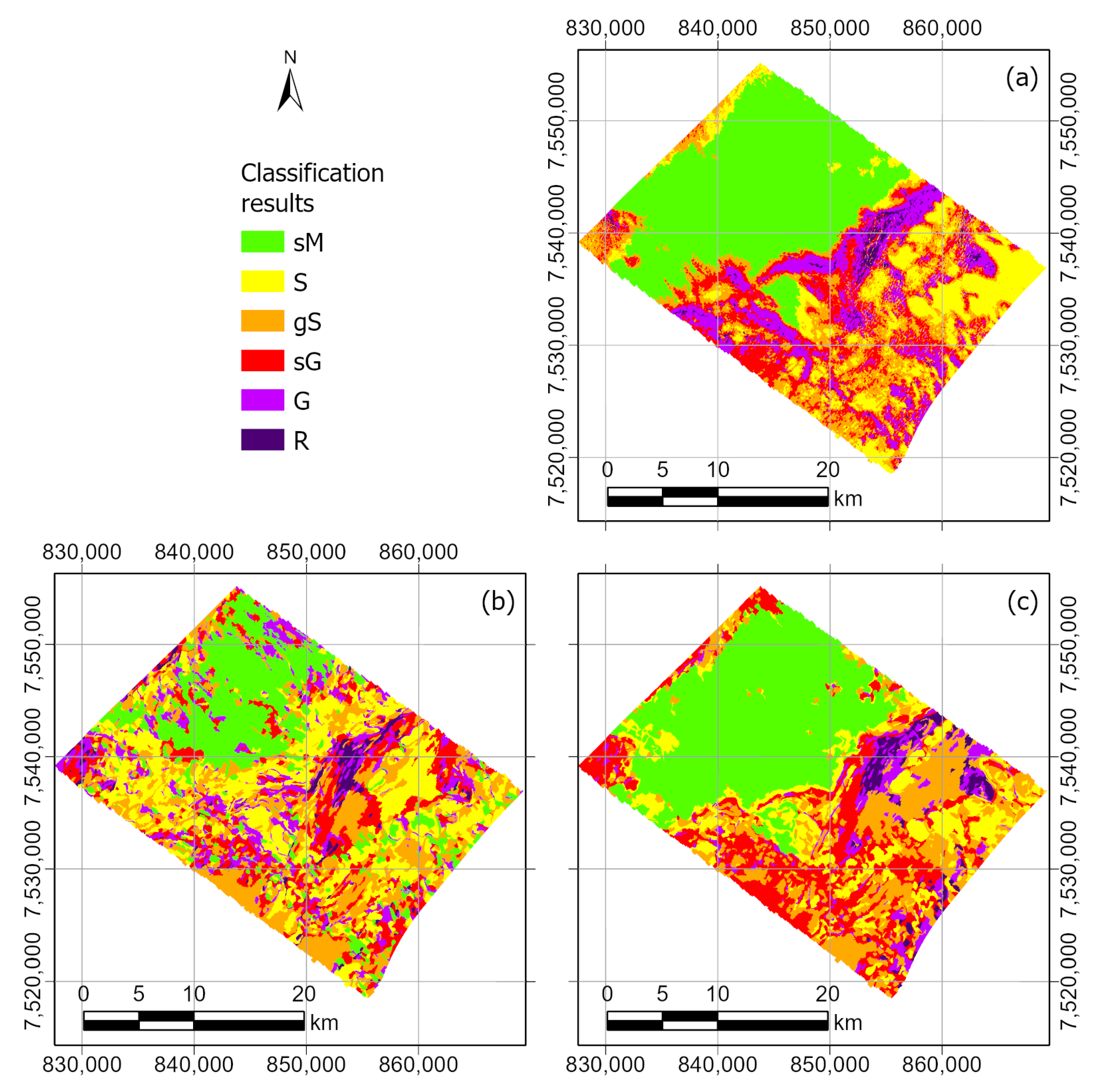
In this section, the classification results are shown. Firstly, Method 1 (see Section 2.2) is applied to the data from the Røstbanken area. These results are then used to validate the results of Methods 2 (Figure 5b) and 3 (Figure 5c). The quality of the classification results from Method 1 is checked by comparison to grab sample ground-reference data (Figure 6). The results from Methods 2 and 3 are compared to grab sample ground-reference data as well, and to the backscatter based results of Method 1. After this, Method 3 is applied to the Borkumer Stones area (Section 3.2).

Figure 5.
Classification maps of the Røstbanken study area: (a) classification based on backscatter data (Method 1); (b) texture features only (Method 2); and (c) texture and layer features (Method 3).

Figure 6.
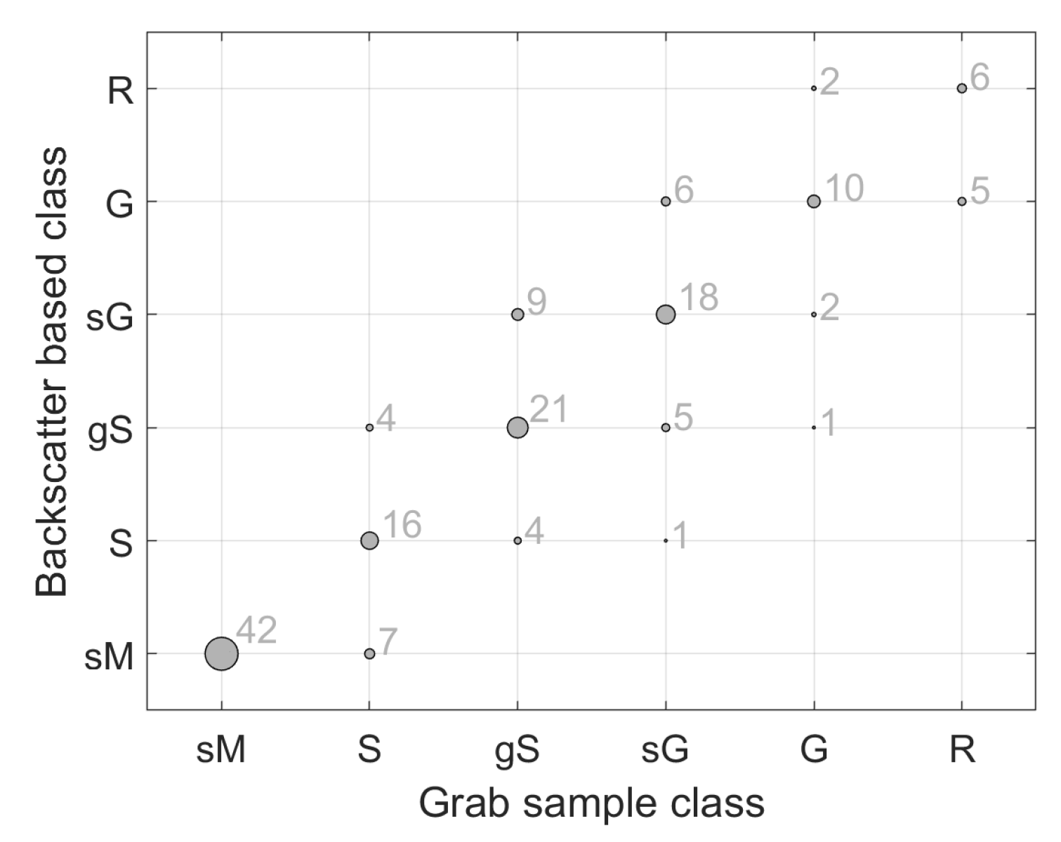
Correlation between backscatter-based classification (Method 1) and sediment type at grab sample locations. Dots, with the associated text, indicate the number of matches between classification and sediment type. The error matrix is shown in Table 3.
3.1. Røstbanken Results
3.1.1. Method 1, Backscatter Based Classification
Firstly, a baseline classification is established by the use of Method 1 (Figure 5a). For this classification, thresholds on the different layers are used to classify the area. The most prominently used layer is the backscatter layer. Aside from backscatter, bathymetry is also used repeatedly and the within object standard deviation of is used once.
The deeper northwestern half (Figure 1a) of the study area has the largest area of uniform sediment, of type sandy mud (sM, Figure 5). On the northwestern edge of the study area, some coarser mixed sediments are also found. In the southeastern half of the study area, a mixture of sediments is found ranging from sand to rock.
When these classification results are compared to the ground-reference data (Figure 6 and Table 3), it is seen that there is a good agreement. For each sediment type, the classification matches the grab sample type the majority of the time. Overall, 71 % of the time the match was perfect, and 98.7 % of the time the classification was within class of the grab sample type.

Table 3.
Error matrix comparing backscatter-based class to grab sample based class. The data are also shown in Figure 6.
3.1.2. Method 2, Classification Using Only Textural Image Object Features
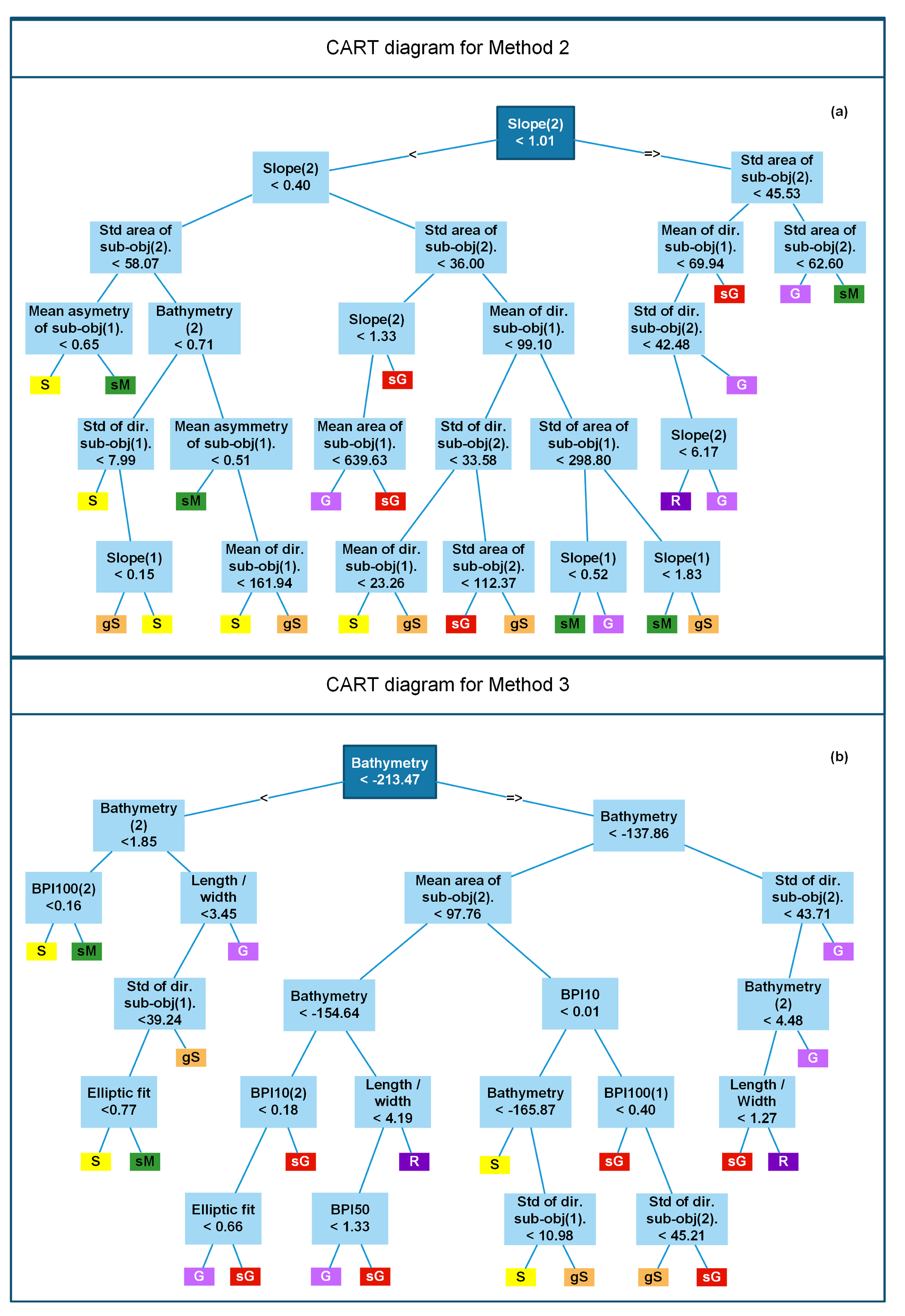
Next, Method 2, a texture only-based classification, is performed (Figure 5b). For this method, none of the layers mentioned in Section 2.1.1 are directly referenced. Rather, texture-related image object features are used. The backscatter layer is not used at any point, that is, not in the classification and also not in the segmentation stage, of the procedure. The segmentation was carried out with the layers and layer weights given in Table 2. The CART utilized 11 different object features at 24 different nodes (Figure 7a and Table 4). The object feature as well as its deciding value is given for each node in Figure 7. Left branches are followed if the values are less than the value indicated at the node. Right branches are followed if the values are equal to or greater than the decision point. The leaves of the tree indicate the class label for the image object in question. Table 4 gives a description of each of the image object features that are used in the CART.
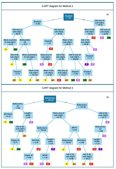
Figure 7.
(a) Diagram of the CART for texture only based classification (Method 2) (see Figure 5b). (b) Diagram of the CART for texture and layer based classification (Method 3) (see Figure 5c). Text in each box indicates the object feature used and its value for the decision rule. Left branches indicate the less than direction and right branches indicate the greater than or equal to direction.

Table 4.
A list of each of the image object features that formed a node in the CART of Figure 7a. The number of times each of these object features appears as a node is also listed, as well as a description of what the object feature is.
When using only texture-based image object features (Method 2), the resulting classification map is mixed. The large sM area (northwest half of the research area, Figure 5a) is distinguishable (Figure 5b). There is also a rocky area close to 7,540,000 N and 854,000 E that is resolved well with this method. However, the large sM area is not cleanly classified as sM, but has small areas that are classified as harder substrate, up to and including gravel. In the mixed sediment area (southeast), there is a trend of the coexistence of harder and softer substrates in agreement with Figure 5a. However, the exact spatial occurrence of classes differs between the two maps.
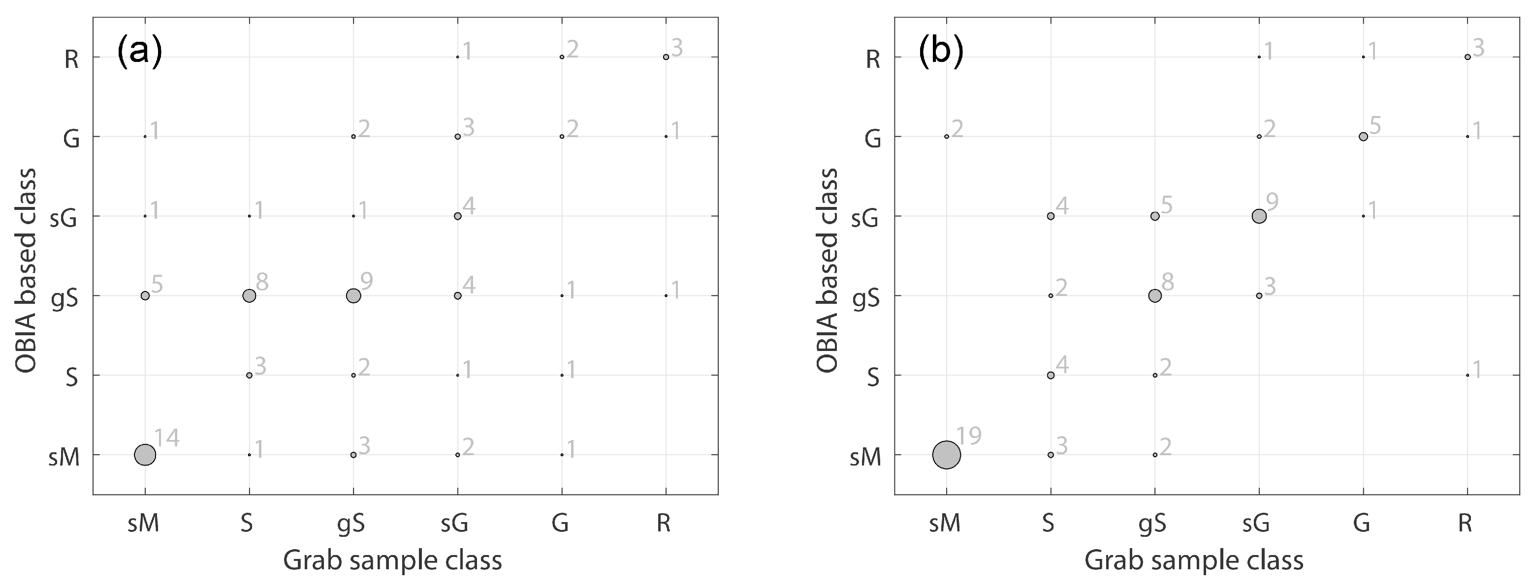
For the results shown in Figure 5b, all the grab samples were used for training the CART. To further assess the performance of Method 2, a different approach is also taken, where the grab sample dataset is subdivided into non-overlapping training and validation subsets. Figure 8a explicitly shows the correlation between the classification and the grab samples. The area around sand grab samples is seen to be classified as gravely sand more often than as sand. Sandy gravel areas, in turn, are just as likely to be classified as gravely sand and almost as likely to be classified as gravel. Of the 78 validation grab samples, the texture-based classification produced a perfect match 35 times, or with 45% accuracy (Table 5 and Figure 8a). The classification was accurate to class 57 times, or 73% of the time.
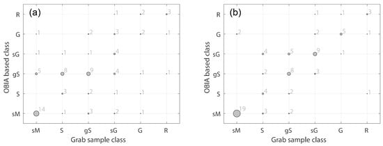
Figure 8.
(a) Correlation between classification results from Method 2 and sediment type at grab sample locations. (b) Correlation between classification results from Method 3 and sediment type at grab sample locations. Corresponding error matrices are shown in Table 5 and Table 7.

Table 5.
Error matrix comparing classification results using Method 2 to grab sample based class. The data are also shown in Figure 8a.
3.1.3. Method 3, Classification Using Image Object Parameters and Non Backscatter Data
A significant improvement in classification is achieved, still not using the backscatter data, when referencing the image layer values directly, during the implementation of Method 3 (Figure 5c). The image object features and deciding values of the CART are seen in Figure 7b. How many times each feature is used and a description of what the features represent are given in Table 6.

Table 6.
A list of each of the image object features that formed a node in the CART of Figure 7b. The number of times each of these object features appears as a node is also listed, as well as a description of what the object feature is.
When the classification is compared to ground-reference data, the improvement to Method 2 becomes clear (Figure 8b). For every grab type, except sand, the majority of the classification classes match the grab sample class. For sand, the classification results was equally likely to be sandy gravel. Of the 78 grab samples, the classification matched exactly 48 times (or 61%) (Table 7 and Figure 8b) and (or 87%) the classification results were within class of the grab sample class 68 times.

Table 7.
Error matrix comparing classification results using Method 3 to grab sample based class. The data are also shown in Figure 8b.
3.1.4. Comparing Non-Backscatter Based Classification to Backscatter Based Classification
Assuming that the backscatter-based classification is accurate, then we can compare the results from Methods 2 and 3 with the backscatter-based classification results from Method 1, in a pixel-by-pixel comparison. For the area that has a specific class based on Method 1, Figure 9 shows, by percentage, how those areas were classified by Methods 2 and 3. Figure 9a shows this relationship where the results of Method 3 are compared to the results from Method 1. Figure 9b shows the results of Method 2 compared to the results of Method 1.
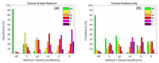
Figure 9.
(a) Comparison of class result from Method 3 for areas having a specific class based on Method 1. (b) Comparison of class result from Method 2 for areas having a specific class based on Method 1.
When using Method 3, the sM area was correctly classified above 90% of the time. For the rest of the classes, the correct classification was between 30% and just over 40%. The percentage of correct classification with a tolerance of class was 86% for the entire area. Per sediment type, it was as follows: sandy mud 92%, sand 81%, gravely sand 86%, sandy gravel 83%, gravel 77%, and rock 73%.
For Method 2 (Figure 9b), the results were not as good. Only sandy mud was correctly classified most of the time. The class percentage was 52% for the entire area, and per sediment type it was as follows: sandy mud 86%, sand 55%, gravely sand 59%, sandy gravel 71%, gravel 60%, and rock 8%.
3.2. Borkumer Stones Results
By using the Røstbanken dataset where backscatter, a good sampling of grab samples, and high quality bathymetry data were available to develop a bathymetry and bathymetric derivative OBIA-based classification method, insights into the performance of the OBIA classification method were obtained. These insights can be applied to the DCS dataset. Based on its performance, Method 3 was used. However, some minor changes to the scale parameter were needed. This was done in order to have the first two levels of image objects conform to small-scale features, as was the case for the Røstbanken data.
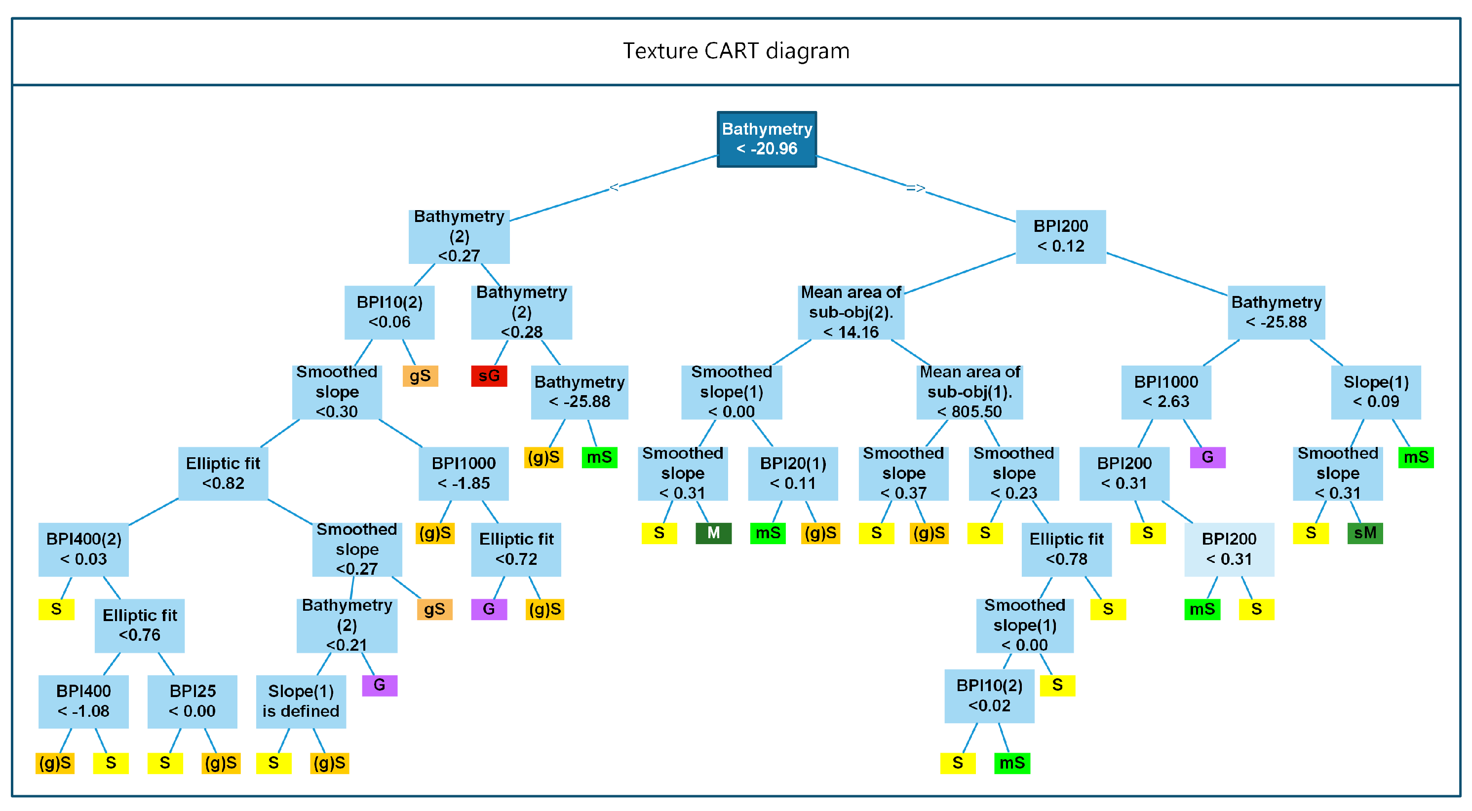
For the Bokumer Stones area, a very similar CART was trained as for the Røstbanken data. The branches and leaves, along with the layer at each node, including the deciding value, are shown in Figure 10. The object features that were used in the CART, along with their description, and the number of times each feature was referenced in the CART are presented in Table 8.

Figure 10.
Diagram of the CART for the classification in the Borkumer Stones area. Text in each box indicates the object feature used and its value for the decision rule. Left branches indicate the less than direction and right branches indicate the greater than or equal to direction.

Table 8.
A list of each of the image object features that formed a node in the CART of Figure 10. The number of times each of these object features appears as a node is also listed, as well as a description of what the object feature is.
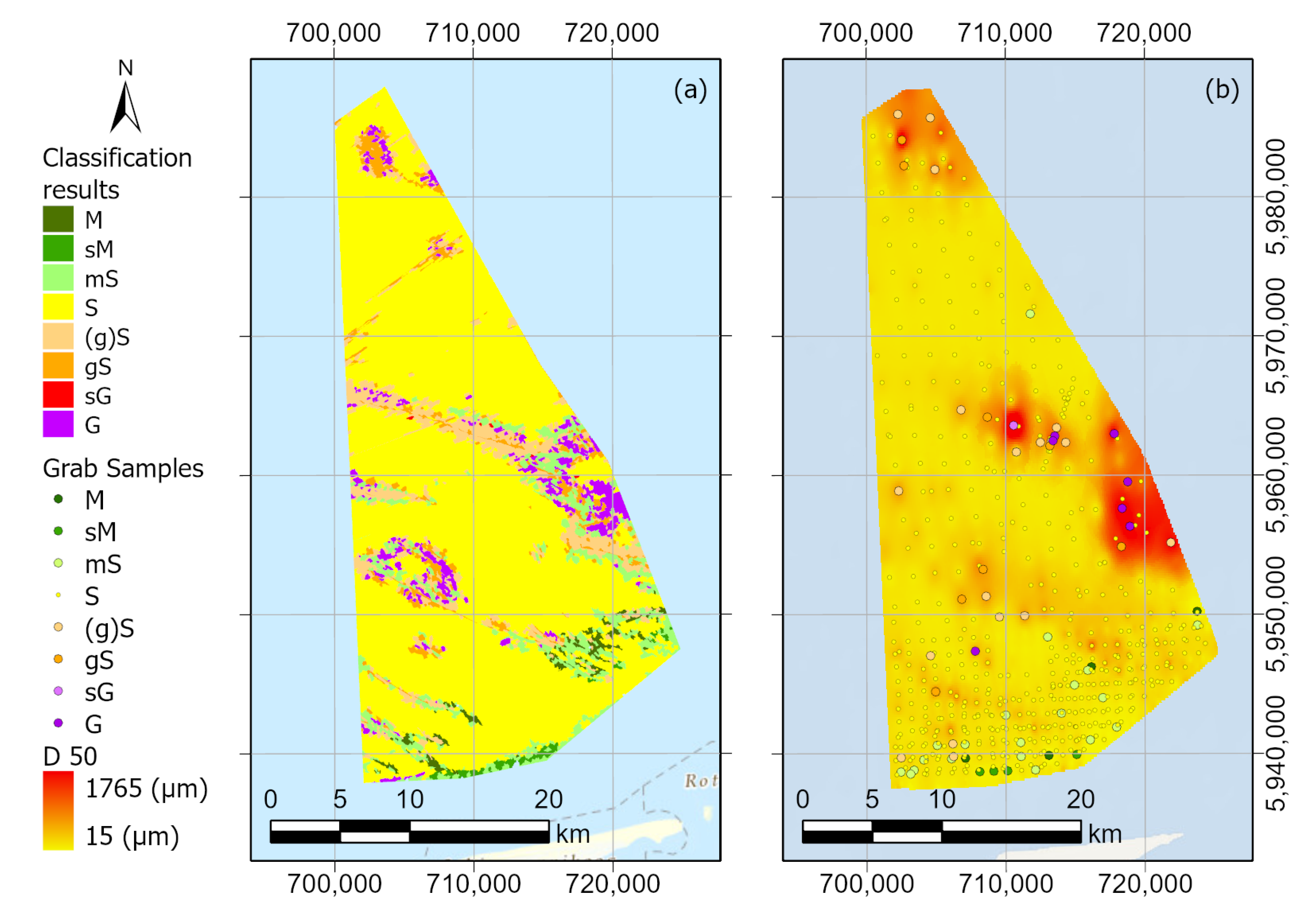
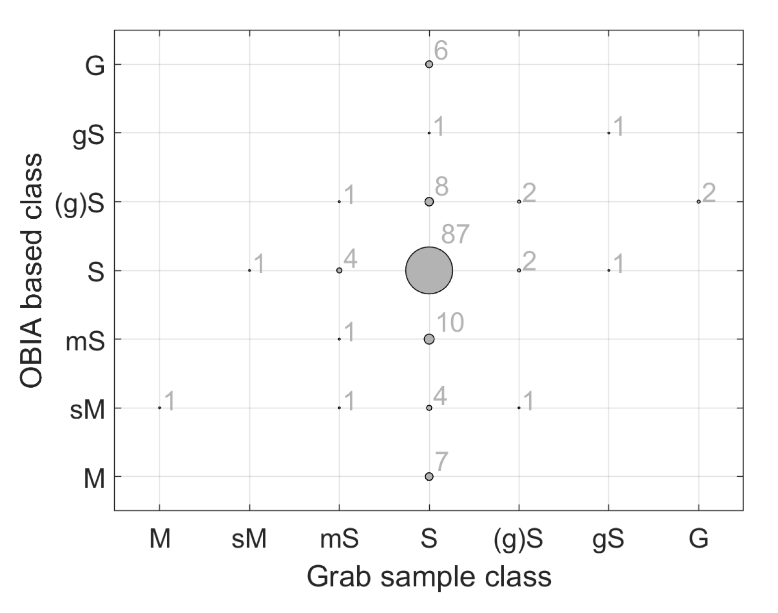
To ground truth the classification results (Figure 11a) with grab sample data, the grab samples were divided into training and validation sets. In the validation set, there were 139 grab samples, of which 123 were of class sand (Figure 12). For 91 of the 139 samples (65%), there was a perfect match between the OBIA class and the grab sample class (Table 9 and Figure 12). For 117 of the samples (or 84%), the OBIA results were within class of the grab sample class.
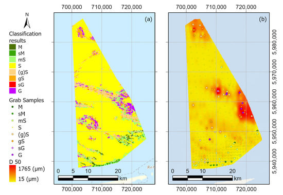
Figure 11.
(a) Classification results from the Borkumer Stones area of the Dutch North Sea. (b) A D50 map interpolated from grab samples. Grab sample locations are shown classified according to Folk.
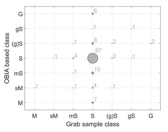
Figure 12.
Texture-based classification results from the Borkumer Stones area compared to grab sample ground-reference data. The error table for these results is given in Table 9.

Table 9.
Error matrix comparing classification results, from the Borkumer Stones area, using Method 3 to grab sample based class. The data are also shown in Figure 12.
For the Røstbanken area, it was possible to compare the OBIA classification results to results from a separate classification method based on backscatter (Method 1). However, for the Borkumer Stones area, backscatter was not available. Although a comparison to grab sample ground-reference data was made, it would be preferable to also have a second comparison method. For this, a different feature of the ground-reference data was used, namely the D50 values, which are similar to the Folk classes that were used to train the CART, but not identical. These are used to generate a second full coverage map for comparison. This map, shown in Figure 11b, is a Kriging-based interpolation of the D50 values of the grab samples. By visual comparison of Figure 11a,b, large-scale trends are found to agree.
4. Discussion
4.1. The Performance of OBIA Methods
One of the research questions addressed in this paper is if a fast and reliable texture-based classification method can be found. It should be noted that there is a family of texture-based methods, such as those based on Haralick texture features, that are commonly used in the literature which were not tested. This is because these methods tend to be exceedingly computationally intensive [58,59] and the interest is in a fast method. Therefore, an OBIA approach was investigated. For this research, the software package eCognition was used. Once the rule sets for the OBIA-based classification were developed, the methods were applied to a dataset covering hundreds of square kilometers in a matter of minutes. Because of the speed of the OBIA methods, they were well suited to get a rapid overview of large areas of the seafloor. It should be noted that the OBIA methods were only used on image datasets with a resolution of 5 m × 5 m. Of the different stages of the classification process, the segmentation stage was the most computationally expensive. The run-time of the multi segmentation algorithm grows linearly with an increase in number of pixels [60]. Given the run times of Methods 2 and 3 with the datasets used in this study, it is expected that, for datasets covering areas up to the entire DCP (59,000 km) at resolutions currently available (5–25 m pixel sizes) [24], this algorithm would remain well suited when used on modern high performance desktop computers (Quad core processor or better, 64 GB of RAM or better). However, if the method were applied to datasets that either cover much larger areas or have a much higher resolution than those mentioned in this paper, then computation time and memory bottlenecks would need to be considered [61].
As far as the reliability of the classification results are concerned, the two methods that were developed in this paper (Methods 2 and 3, Section 2.2) had differing reliability results. When compared to grab samples, classification accuracies of 98.7%, 73%, and 87% were achieved with a tolerance of class for Methods 1–3, respectively. Assuming Method 1 to yield a correct classification allowed for Methods 2 and 3 to be compared to it on a pixel by pixel bases. When this was done, Methods 2 and 3 had an accuracy of 52% and 86%, respectively, again with a tolerance of classes. Since the layer and grab sample inputs for Methods 2 and 3 are the same, and given the fact that they differed little in computational requirements, the use of Method 3 is recommended instead of Method 2. However, the texture features that Method 2 is based on should certainly be included in future OBIA methods. This is recommended based on the fact that they were included in Method 3 and were used for almost half of the nodes of the CART of Method 3 (Figure 7b and Table 6).
4.2. Application of the Algorithm to Different Datasets
A testament to the robustness of the OBIA methods developed in this paper is the fact that very little needed changing when Method 3 was applied to a different dataset in order to achieve good classification results. Some changes were necessary for the image objects at Levels 1 and 2 to conform to the shape of small-scale seafloor features. To accomplish this, the scale parameter was adjusted for these two levels of image segmentation. The weights of the image layers used during the segmentation was also adjusted to utilize the best layers for the given area. This indicates that, as long as image objects are allowed to conform to the shapes of small-scale seafloor features at the lower levels of image objects, then this method remains applicable to new datasets.
4.3. The Affect of Bathymetry Flaws
From the data that were used in this research, the dataset from the Borkumer Stones area had some bathymetric flaws. These errors were likely the result of uncorrected or poorly corrected motion sensor or lever arm artifacts [45]. The artifacts were consistent in their across track, along track, and sailing direction specific patterns that is typical of this kind of error. Because of these flaws, there were some areas where the lower level image objects conformed to artifacts instead of to real seafloor features. This may explain why the classification from the Borkumer Stones data, when compared to grab sample ground-reference, was not quite as good as the results for the Røstbanken data (when using an accuracy measure of ±1 acoustic class). Because of the OBIA-based classification method’s reliance on image objects conforming to actual seafloor features, clean bathymetry data are of high importance for the classification method developed in this paper.
4.4. Good Use-Cases for Bathymetry Based OBIA Based Classification
Because of the need for up-to-date navigational charts, many countries collect high-resolution bathymetry data covering big sections of their territorial waters on regularly scheduled intervals [24]. This means that high-quality bathymetry data are widely available. Furthermore, as a part of the 2030 project, high-resolution bathymetry data will become available for the entirety of the world’s oceans [27]. Unlike bathymetry, backscatter data remain much harder to come by.
It is difficult to quantify the ratio of the seafloor for which bathymetry is available but backscatter is not. There is little focus on the gathering of backscatter at the global scale, and with good reason, as even the well-funded and well-organized MAREANO, Norway’s national offshore mapping program, had difficulty dealing with the size of such backscatter datasets [62]. Of the efforts to collect full coverage backscatter data, MAREANO is a good example, as well as Germany where side scan sonars are widely used [63,64]. For the DCS, full coverage bathymetry data are available via EMODnet [25]. In addition to this, bathymetry data up to a resolution of 25 m m (and in some cases 5 m m), can be requested of the Hydrographic Service of the Royal Netherlands Navy. The Navy surveys the entirety of the DCS on scheduled intervals. Backscatter is not available through any of these means. The Royal Netherlands Institute for Sea Research (NIOZ) can at any moment have some backscatter data available, but they do not have a long-term storage plan for backscatter data gathered during their cruises. An example where backscatter data were made available by the RVO on the DCS is the case of the “De Rijke Noordzee”, who were able to analyze ~1200 km that was gathered during surveys for the placing of wind farms [26]. Because there is no centralized gathering point for backscatter data, it is difficult to quantify the area for which backscatter data exist for many regional coastal waters, while it is well known that full coverage bathymetry exists.
At the global scale, there are organized efforts, especially after the disappearance of Malaysia Airlines flight MH370 and the subsequent search, to collect bathymetry data [27,65]. Due to this, there are also good estimates on how much of the global seafloor has been measured by echosounders, and it is less than 18% [27]. The fact that backscatter is much less available is also demonstrated by the fact that it is not even mentioned in these efforts [27,65]. This is further confirmed by the fact that the standardization for the acquisition and interpretation of backscatter data is still a very active field of research [23].
Because bathymetry is more readily available than backscatter, it is desirable to develop fast and accurate classification methods that do not rely on backscatter data. Such methods could then be applied in order to provide classification results of large areas of many European and American coastal seas, among others. When full coverage bathymetry data of the entire globe become available, such methods can then be applied at the global scale. Although backscatter-based classification still yields better results, OBIA classification results using only bathymetry and its derivatives yielded classification results with a 10% loss in accuracy. As such, the methods developed in this paper should be considered as good options in circumstances where backscatter data are not available.
5. Summary and Conclusions
In this study, two seafloor classification methods were developed that use an OBIA approach. The methods use bathymetry, bathymetric derivatives, and grab samples as input, and they do not rely on the use of backscatter. The transferability of the best method was tested by applying it to two datasets. The first dataset was from Norwegian waters, specifically the Røstbanken area off the coast of Lofoten. The second dataset was from Borkumer Stones area close to the island of Schiermonnikoog in Dutch waters. The classification results were compared to the results from an existing backscatter-based classification method (Method 1) in the case of the Røstbanken data, and to grab sample ground-reference data for both datasets.
The first of the developed methods (Method 2) used a purely texture-based OBIA approach. The second method (Method 3) was similar, but used additional image object features. Both methods are fast enough to be used over large coastal areas with data resolutions of 5 m × 5 m. To apply the method(s) to new areas, adjustments to the scale parameter of the segmentation algorithm were necessary. Additionally, when creating the first two levels of image objects, image layer choice was important in order for the shapes of the image objects to conform to small scale features of the seafloor. With these adjustments, the algorithm was transferable to new research areas.
When comparing Methods 1–3 to grab sample ground-reference data, a respective classification accuracy of 98.7%, 73%, and 87% was found when a tolerance of class was used. When only perfect matches are considered, then the accuracies are 71%, 45%, and 61%, respectively. When compared to the results from Method 1, Method 2 had an accuracy of 52% and Method 3 an accuracy of 86% with a class tolerance. Because the input requirements and computation cost do not differ significantly between Methods 2 and 3, the use of Method 3 is recommended.
Having a bathymetry and bathymetric derivative-based classification method is important given that bathymetry data are more available than backscatter data for many coastal seas. This importance is even greater when considering full global coverage of bathymetric data being available through projects such as the GEBCO seabed 2030 project [27]. As such, the results presented in this paper should be of wide interest to the seafloor classification community.
Author Contributions
Conceptualization, L.K., M.S. and D.G.S. methodology, L.K. and M.S.; software, L.K. and M.S.; formal analysis, L.K. and M.S.; investigation, L.K.; resources, L.K., M.S. and D.G.S.; data curation, L.K.; writing—original draft preparation, L.K., and M.S.; writing—review and editing, L.K., M.S. and D.G.S.; visualization, L.K. and M.S.; supervision, M.S. and D.G.S.; project administration, L.K., M.S. and D.G.S.; and funding acquisition, M.S. and D.G.S. All authors have read and agreed to the published version of the manuscript.
Funding
This research is part of the multidisciplinary research project DISCLOSE. DISCLOSE is a joint venture of the Delft University of Technology, the University of Groningen, the Royal Netherlands Institute for Sea Research, as well as the North Sea Foundation. DISCLOSE is funded by the Gieskes Strijbis Fonds.
Data Availability Statement
The data presented in this study are available on request from the corresponding author. The data are not publicly available due to agreements with third parties.
Acknowledgments
The authors would like to acknowledge Markus Diesing and his colleagues at CEFAS for their work in acquiring and processing the Røstbanken dataset. The organizers of the GeoHab 2016 workshop, where the Røstbanken data were made available, are also acknowledged [35]. Leendert Dorst and Daniëlle van Kuijk of the Hydrographic Service within the Royal Netherlands Navy are thanked for making full coverage, high resolution bathymetric data available from the Borkumer Stones area. Finally, Sytze van Heteren of TNO is acknowledged for making the grab sample data for the Borkumer Stones available for this research [41]. The EMODnet-Geology [66], TILES [67], and AufMod [68] projects are further recognized for their part in the compilation of the grab sample data.
Conflicts of Interest
The authors declare no conflict of interest. The funders had no role in the design of the study; in the collection, analyses, or interpretation of data; in the writing of the manuscript, or in the decision to publish the results.
Abbreviations
The following abbreviations are used in this manuscript:
| CART | Classification and regression tree |
| DCS | Dutch continental shelf |
| DISCLOSE | Distribution, Structure and functioning of low resilience benthic communities and habitats of the Dutch North Sea |
| EMODNet | European Marine Observation and Data Network |
| GPS | Global positioning system |
| m | Meter |
| MBES | Multibeam echosounder |
| MRU | Motion reference unit |
| NIOZ | Royal Netherlands Institute for Sea Research |
| OBIA | Object-based image analysis |
| QPS | Quality Positioning Systems |
| RVO | Rijksdienst voor Ondernemend Nederland (Netherlands Enterprise Agency) |
References
- Blake, J. The Sea Chart: The Illustrated History of Nautical Maps and Navigational Charts; Anova Books: London, UK, 2009. [Google Scholar]
- Monahan, D. Bathymetry. In Encyclopedia of Ocean Sciences, 2nd ed.; Steele, J.H., Ed.; Academic Press: Oxford, UK, 2009; pp. 297–304. [Google Scholar] [CrossRef]
- Brown, C.J.; Smith, S.J.; Lawton, P.; Anderson, J.T. Benthic habitat mapping: A review of progress towards improved understanding of the spatial ecology of the seafloor using acoustic techniques. Estuar. Coast. Shelf Sci. 2011, 92, 502–520. [Google Scholar] [CrossRef]
- Koop, L.; Amiri-Simkooei, A.; van der Reijden, K.J.; O’Flynn, S.; Snellen, M.; Simons, D.G. Seafloor Classification in a Sand Wave Environment on the Dutch Continental Shelf Using Multibeam Echosounder Backscatter Data. Geosciences 2019, 9, 142. [Google Scholar] [CrossRef]
- Simons, D.G.; Snellen, M. A Bayesian approach to seafloor classification using multi-beam echo-sounder backscatter data. Appl. Acoust. 2009, 70, 1258–1268. [Google Scholar] [CrossRef]
- Snellen, M.; Gaida, T.C.; Koop, L.; Alevizos, E.; Simons, D.G. Performance of Multibeam Echosounder Backscatter-Based Classification for Monitoring Sediment Distributions Using Multitemporal Large-Scale Ocean Data Sets. IEEE J. Ocean. Eng. 2019, 44, 142–155. [Google Scholar] [CrossRef]
- Lamarche, G.; Lurton, X.; Verdier, A.L.; Augustin, J.M. Quantitative characterisation of seafloor substrate and bedforms using advanced processing of multibeam backscatter—Application to Cook Strait, New Zealand. Cont. Shelf Res. 2011, 31, S93–S109. [Google Scholar] [CrossRef]
- Gaida, T.; Tengku Ali, T.; Snellen, M.; Amiri-Simkooei, A.; van Dijk, T.; Simons, D. A Multispectral Bayesian Classification Method for Increased Acoustic Discrimination of Seabed Sediments Using Multi-Frequency Multibeam Backscatter Data. Geosciences 2018, 8, 455. [Google Scholar] [CrossRef]
- Brown, C.J.; Beaudoin, J.; Brissette, M.; Gazzola, V. Multispectral multibeam echo sounder backscatter as a tool for improved seafloor characterization. Geosciences 2019, 9, 126. [Google Scholar] [CrossRef]
- Ojeda, G.Y.; Gayes, P.T.; Van Dolah, R.F.; Schwab, W.C. Spatially quantitative seafloor habitat mapping: Example from the northern South Carolina inner continental shelf. Estuar. Coast. Shelf Sci. 2004, 59, 399–416. [Google Scholar] [CrossRef]
- Marsh, I.; Brown, C. Neural network classification of multibeam backscatter and bathymetry data from Stanton Bank (Area IV). Appl. Acoust. 2009, 70, 1269–1276. [Google Scholar] [CrossRef]
- Stephens, D.; Diesing, M. A comparison of supervised classification methods for the prediction of substrate type using multibeam acoustic and legacy grain-size data. PLoS ONE 2014, 9, e93950. [Google Scholar] [CrossRef] [PubMed]
- McGonigle, C.; Brown, C.; Quinn, R.; Grabowski, J. Evaluation of image-based multibeam sonar backscatter classification for benthic habitat discrimination and mapping at Stanton Banks, UK. Estuar. Coast. Shelf Sci. 2009, 81, 423–437. [Google Scholar] [CrossRef]
- McGonigle, C.; Grabowski, J.H.; Brown, C.J.; Weber, T.C.; Quinn, R. Detection of deep water benthic macroalgae using image-based classification techniques on multibeam backscatter at Cashes Ledge, Gulf of Maine, USA. Estuar. Coast. Shelf Sci. 2011, 91, 87–101. [Google Scholar] [CrossRef]
- Brown, C.J.; Todd, B.J.; Kostylev, V.E.; Pickrill, R.A. Image-based classification of multibeam sonar backscatter data for objective surficial sediment mapping of Georges Bank, Canada. Cont. Shelf Res. 2011, 31, S110–S119. [Google Scholar] [CrossRef]
- Eleftherakis, D.; Amiri-Simkooei, A.; Snellen, M.; Simons, D.G. Improving riverbed sediment classification using backscatter and depth residual features of multi-beam echo-sounder systems. J. Acoust. Soc. Am. 2012, 131, 3710–3725. [Google Scholar] [CrossRef] [PubMed]
- Eleftherakis, D.; Snellen, M.; Amiri-Simkooei, A.; Simons, D.G.; Siemes, K. Observations regarding coarse sediment classification based on multi-beam echo-sounder’s backscatter strength and depth residuals in Dutch rivers. J. Acoust. Soc. Am. 2014, 135, 3305–3315. [Google Scholar] [CrossRef]
- Amiri-Simkooei, A.; Snellen, M.; Simons, D.G. Riverbed sediment classification using multi-beam echo-sounder backscatter data. J. Acoust. Soc. Am. 2009, 126, 1724–1738. [Google Scholar] [CrossRef]
- Van Der Reijden, K.J.; Koop, L.; O’flynn, S.; Garcia, S.; Bos, O.; Van Sluis, C.; Maaholm, D.J.; Herman, P.M.; Simons, D.G.; Olff, H. Discovery of Sabellaria spinulosa reefs in an intensively fished area of the Dutch Continental Shelf, North Sea. J. Sea Res. 2019, 144, 85–94. [Google Scholar] [CrossRef]
- Blondel, P.; Sichi, O.G. Textural analyses of multibeam sonar imagery from Stanton Banks, Northern Ireland continental shelf. Appl. Acoust. 2009, 70, 1288–1297. [Google Scholar] [CrossRef]
- Clarke, J.E.H. Multispectral acoustic backscatter from multibeam, improved classification potential. In Proceedings of the United States Hydrographic Conference, San Diego, CA, USA, 21–24 September 2015; pp. 15–19. [Google Scholar]
- Vas, E. MultiSpectral Mode™ Survey Capability. 2016. Available online: https://www.r2sonic.com/multispectral-mode-survey-capability/ (accessed on 15 November 2016).
- Lamarche, G.; Lurton, X. Recommendations for improved and coherent acquisition and processing of backscatter data from seafloor-mapping sonars. Mar. Geophys. Res. 2018, 39, 5–22. [Google Scholar] [CrossRef]
- Navy, R.N. Online Availability of Data of the Netherlands Hydrographic Service. Available online: https://english.defensie.nl/topics/hydrography/documents/letters/2020/06/24/online-availability-of-data-from-the-hydrographic-service (accessed on 7 July 2020).
- Developing and Providing a Harmonised Digital Terrain Model (DTM) for the European Sea Regions. Available online: https://www.emodnet-bathymetry.eu/ (accessed on 13 January 2021).
- Gaida, T.C. Onderzoek naar Zeebodem in de Noordzee. Available online: https://www.derijkenoordzee.nl/nieuws/onderzoek-naar-zeebodem-in-de-noordzee (accessed on 13 January 2021).
- Mayer, L.; Jakobsson, M.; Allen, G.; Dorschel, B.; Falconer, R.; Ferrini, V.; Lamarche, G.; Snaith, H.; Weatherall, P. The Nippon Foundation—GEBCO seabed 2030 project: The quest to see the world’s oceans completely mapped by 2030. Geosciences 2018, 8, 63. [Google Scholar] [CrossRef]
- Diesing, M.; Mitchell, P.; Stephens, D. Image-based seabed classification: What can we learn from terrestrial remote sensing? ICES J. Mar. Sci. 2016, 73, 2425–2441. [Google Scholar] [CrossRef]
- Blaschke, T. Object based image analysis for remote sensing. ISPRS J. Photogramm. Remote Sens. 2010, 65, 2–16. [Google Scholar] [CrossRef]
- Diesing, M.; Green, S.L.; Stephens, D.; Lark, R.M.; Stewart, H.A.; Dove, D. Mapping seabed sediments: Comparison of manual, geostatistical, object-based image analysis and machine learning approaches. Cont. Shelf Res. 2014, 84, 107–119. [Google Scholar] [CrossRef]
- Janowski, Ł.; Tęgowski, J.; Nowak, J. Seafloor mapping based on multibeam echosounder bathymetry and backscatter data using Object-Based Image Analysis: A case study from the Rewal site, the Southern Baltic. Oceanol. Hydrobiol. Stud. 2018, 47, 248–259. [Google Scholar] [CrossRef]
- Lacharité, M.; Brown, C.J.; Gazzola, V. Multisource multibeam backscatter data: Developing a strategy for the production of benthic habitat maps using semi-automated seafloor classification methods. Mar. Geophys. Res. 2018, 39, 307–322. [Google Scholar] [CrossRef]
- Menandro, P.S.; Bastos, A.C.; Boni, G.; Ferreira, L.C.; Vieira, F.V.; Lavagnino, A.C.; Moura, R.L.; Diesing, M. Reef Mapping Using Different Seabed Automatic Classification Tools. Geosciences 2020, 10, 72. [Google Scholar] [CrossRef]
- Le Bas, T.P. RSOBIA—A New OBIA Toolbar and Toolbox in ArcMap 10. x for Segmentation and Classification. Available online: https://www.researchgate.net/profile/Tim_Le_Bas/publication/311315300_RSOBIA_-_A_new_OBIA_Toolbar_and_Toolbox_in_ArcMap_10x_for_Segmentation_and_Classification/links/584e755708aecb6bd8cd5a98/RSOBIA-A-new-OBIA-Toolbar-and-Toolbox-in-ArcMap-10x-for-Segmentation-and-Classification.pdf (accessed on 21 January 2021).
- GeoHab. Marine Environment Mapping and Interpretation-from the Coast to the Deep Ocean, Second Circular. Available online: http://geohab.org/wp-content/uploads/2018/09/Geohab-2016-2nd-Circular.pdf (accessed on 26 May 2020).
- Micallef, A.; Krastel, S.; Savini, A. Submarine Geomorphology; Springer: Berlin, Germany, 2017. [Google Scholar]
- Ottesen, D.; Dowdeswell, J.; Rise, L. Submarine landforms and the reconstruction of fast-flowing ice streams within a large Quaternary ice sheet: The 2500-km-long Norwegian-Svalbard margin (57–80 N). GSA Bull. 2005, 117, 1033–1050. [Google Scholar] [CrossRef]
- Coolen, J.W.; Bos, O.G.; Glorius, S.; Lengkeek, W.; Cuperus, J.; van der Weide, B.; Agüera, A. Reefs, sand and reef-like sand: A comparison of the benthic biodiversity of habitats in the Dutch Borkum Reef Grounds. J. Sea Res. 2015, 103, 84–92. [Google Scholar] [CrossRef]
- Olsen, O.T. The Piscatorial Atlas of the North Sea, English and St. George’s Channels: Illustrating the Fishing Ports, Boats, Gear, Species of Fish (How, Where and When Caught), and Other Information Concerning Fish and Fihseries; OT Olsen: London, UK, 1883. [Google Scholar]
- Dörjes, J. Über die Bodenfauna des Borkum Riffgrundes (Nordsee). Senckenberg. Marit 1977, 9, 1–17. [Google Scholar]
- Valerius, J.; Van Lancker, V.; Van Heteren, S.; Leth, J.; Zeiler, M. Trans-national database of North Sea sediment data. In Data Compilation by Federal Maritime and Hydrographic Agency (Germany); Royal Belgian Institute of Natural Sciences: Brussels, Belgium; TNO: The Hague, The Netherlands; Geological Survey of Denmark and Greenland: Copenhagen, Denmark, 2014. [Google Scholar]
- Stephens, D.; Diesing, M. Towards quantitative spatial models of seabed sediment composition. PLoS ONE 2015, 10, e0142502. [Google Scholar] [CrossRef]
- Esri. World Topographic Map. 2012. Available online: http://www.arcgis.com/home/item.html?id=30e5fe3149c34df1ba922e6f5bbf808f (accessed on 21 January 2021).
- Schimel, A.C.; Beaudoin, J.; Parnum, I.M.; Le Bas, T.; Schmidt, V.; Keith, G.; Ierodiaconou, D. Multibeam sonar backscatter data processing. Mar. Geophys. Res. 2018, 39, 121–137. [Google Scholar] [CrossRef]
- Clarke, J.E.H. Dynamic motion residuals in swath sonar data: Ironing out the creases. Int. Hydrogr. Rev. 2003. Available online: https://www.researchgate.net/publication/242429939_Dynamic_Motion_Residuals_in_Swath_Sonar_Data_Ironing_out_the_Creases (accessed on 21 January 2021).
- Zevenbergen, L.W.; Thorne, C.R. Quantitative analysis of land surface topography. Earth Surf. Process. Landf. 1987, 12, 47–56. [Google Scholar] [CrossRef]
- Moore, I.D.; Grayson, R.; Ladson, A. Digital terrain modelling: A review of hydrological, geomorphological, and biological applications. Hydrol. Process. 1991, 5, 3–30. [Google Scholar] [CrossRef]
- Zaslavsky, D.; Sinai, G. Surface hydrology: I—Explanation of phenomena. J. Hydraul. Div. 1981, 107, 1–16. [Google Scholar]
- Weiss, A. Topographic position and landforms analysis. In Proceedings of the Poster Presentation, ESRI User Conference, San Diego, CA, USA, 9–13 July 2001; Volume 200. [Google Scholar]
- Lundblad, E.R.; Wright, D.J.; Miller, J.; Larkin, E.M.; Rinehart, R.; Naar, D.F.; Donahue, B.T.; Anderson, S.M.; Battista, T. A benthic terrain classification scheme for American Samoa. Mar. Geod. 2006, 29, 89–111. [Google Scholar] [CrossRef]
- Walbridge, S.; Slocum, N.; Pobuda, M.; Wright, D.J. Unified geomorphological analysis workflows with Benthic Terrain Modeler. Geosciences 2018, 8, 94. [Google Scholar] [CrossRef]
- Trimble. eCognition Developer User Guide, 9.2.1 ed.; Trimble: Sunnyvale, CA, USA, 2016. [Google Scholar]
- Benz, U.C.; Hofmann, P.; Willhauck, G.; Lingenfelder, I.; Heynen, M. Multi-resolution, object-oriented fuzzy analysis of remote sensing data for GIS-ready information. ISPRS J. Photogramm. Remote Sens. 2004, 58, 239–258. [Google Scholar] [CrossRef]
- Baatz, M.; Schäpe, A. Multiresolution Segmentation: An Optimization Approach for High Quality Multi-Scale Image Segmentation. Available online: https://pdf4pro.com/view/multiresolution-segmentation-an-optimization-approach-598443.html (accessed on 21 January 2021).
- Trimble. eCognition Developer Reference Book; Trimble: Sunnyvale, CA, USA, 2019. [Google Scholar]
- Jørgensen, B.; Erik, N. (TerraNor, Roa, Norway); Markus, D. (CEFAS, Lowestoft, UK). Personal communication, 2016.
- Breiman, L.; Friedman, J.; Stone, C.; Olshen, R. Classification and Regression Trees; The Wadsworth and Brooks-Cole Statistics-Probability Series; Taylor & Francis: Oxfordshire, UK, 1984. [Google Scholar]
- Zhang, H.; Hung, C.L.; Min, G.; Guo, J.P.; Liu, M.; Hu, X. GPU-Accelerated GLRLM Algorithm for Feature Extraction of MRI. Sci. Rep. 2019, 9, 1–13. [Google Scholar] [CrossRef]
- Doycheva, K.; Koch, C.; König, M. Implementing textural features on GPUs for improved real-time pavement distress detection. J. Real-Time Image Process. 2019, 16, 1383–1394. [Google Scholar] [CrossRef]
- Csillik, O. Fast segmentation and classification of very high resolution remote sensing data using SLIC superpixels. Remote Sens. 2017, 9, 243. [Google Scholar] [CrossRef]
- Csilik, O.; Lang, S. Improving the Speed of Multiresolution Segmentation Using Slic Superpixels; University of Salzburg: Salzburg, Austria, 2016; Available online: http://proceedings.utwente.nl/371/1/Csillik-Improving%20the%20Speed%20of%20Multiresolution%20Segmentation%20Using%20SLIC%20Superpixels-94.pdf (accessed on 21 January 2021).
- Elvenes, S.; Dolan, M.F.; Buhl-Mortensen, P.; Bellec, V.K. An evaluation of compiled single-beam bathymetry data as a basis for regional sediment and biotope mapping. ICES J. Mar. Sci. 2014, 71, 867–881. [Google Scholar] [CrossRef]
- von Nordheim, H.; Wollny-Goerke, K. Progress in Marine Conservation in Europe; Springer: Berlin, Germany, 2015. [Google Scholar]
- Propp, C.; Bartholomä, A.; Hass, C.; Holler, P.; Lambers-Huesmann, M.; Papenmeier, S.; Richter, P.; Schwarzer, K.; Tauber, F.; Zeiler, M. Guideline for Seafloor Mapping in German Marine Waters Using High-Resolution Sonars. 2016. Available online: https://www.bsh.de/download/Guideline-for-Seafloor-Mapping.pdf (accessed on 21 January 2021).
- Wölfl, A.C.; Snaith, H.; Amirebrahimi, S.; Devey, C.W.; Dorschel, B.; Ferrini, V.; Huvenne, V.A.I.; Jakobsson, M.; Jencks, J.; Johnston, G.; et al. Seafloor Mapping–The Challenge of a Truly Global Ocean Bathymetry. Front. Mar. Sci. 2019, 6, 283. [Google Scholar] [CrossRef]
- EMODnet. EMODnet Geology. Available online: https://www.emodnet.eu/geology (accessed on 17 July 2020).
- Van Lancker, V. Transnational and Integrated Long-Term Marine Exploitation Strategies; Belgian Science Policy: Brussels, Belgium, 2019. [Google Scholar]
- Heyer, H.; Schrottke, K.; Pluess, A. Aufbau von integrierten Modellsystemen zur Analyse der Langfristigen Morphodynamik in der Deutschen Bucht; Karlsruhe: Hamburg, Germany, 2014. [Google Scholar]
Publisher’s Note: MDPI stays neutral with regard to jurisdictional claims in published maps and institutional affiliations. |
© 2021 by the authors. Licensee MDPI, Basel, Switzerland. This article is an open access article distributed under the terms and conditions of the Creative Commons Attribution (CC BY) license (http://creativecommons.org/licenses/by/4.0/).

