Site Amplification during Strong Earthquakes Investigated by Vertical Array Records

Abstract

A number of vertical array records during eight destructive earthquakes in Japan are utilized, after discussing criteria for desirable requirements of vertical arrays, to formulate seismic amplification between ground surface and outcrop base for seismic zonation. A correlation between peak spectrum amplification and V_s (S-wave velocity) ratio (base V_s/surface V_s) was found to clearly improve by using V_s in an equivalent surface layer wherein predominant frequency or first peak is exerted, though the currently used average V_s in top 30 m is also meaningful, correlating positively with the amplification. We also found that soil nonlinearity during strong earthquakes has only a marginal effect even in soft soil sites on the amplification between surface and outcrop base except for ultimate soil liquefaction failure, while strong nonlinearity clearly appears in the vertical array amplification between surface and downhole base. Its theoretical basis has been explained by a simple study on a two-layered system in terms of radiation damping and strain-dependent equivalent nonlinearity.

1. Introduction

In determining design motions for superstructures, site amplifications have to be evaluated in soil layers above an engineering bedrock (base layer) at which the design motion is prescribed. The bedrock is defined at stiff bearing strata with S-wave velocities of around V_s = 400~700 m/s or larger, normally. The incident earthquake motions are evaluated from fault mechanisms and attenuations along wave paths from faults to particular sites for individual earthquakes. Then, the evaluation of seismic amplification due to different site conditions is essential in developing hazard maps for local governments.

In evaluating the site amplification, the soil profile is simplified by a one-dimensional model unless it is very variable in geology or topography. Horizontal shear wave (SH-wave) propagating in the horizontally-layered soil deposits is first considered because of its significant effect on geotechnical engineering problems, although other wave types have to be considered in more heterogeneous or topographically complex site conditions. The appreciation of the significant role of the SH-wave in site amplification stems from the pioneering work by Kanai et al. in 1956 [1] and 1966 [2], wherein simultaneous earthquake observations were conducted at the ground surface and the subsurface level below in a tunnel, demonstrating that seismic horizontal ground motions can be idealized essentially by the SH-wave vertically propagating in one-dimensional horizontal layers.

The site amplification in the 1D soil profile seems to depend on S-wave velocities, soil densities, internal damping of the individual layers. Furthermore, strain-dependent nonlinear properties may affect the amplification in soft soils in focal areas during strong earthquakes. Among the influencing factors, the ratio of S-wave velocities between a bedrock or base layer and a surface layer is of utmost importance.

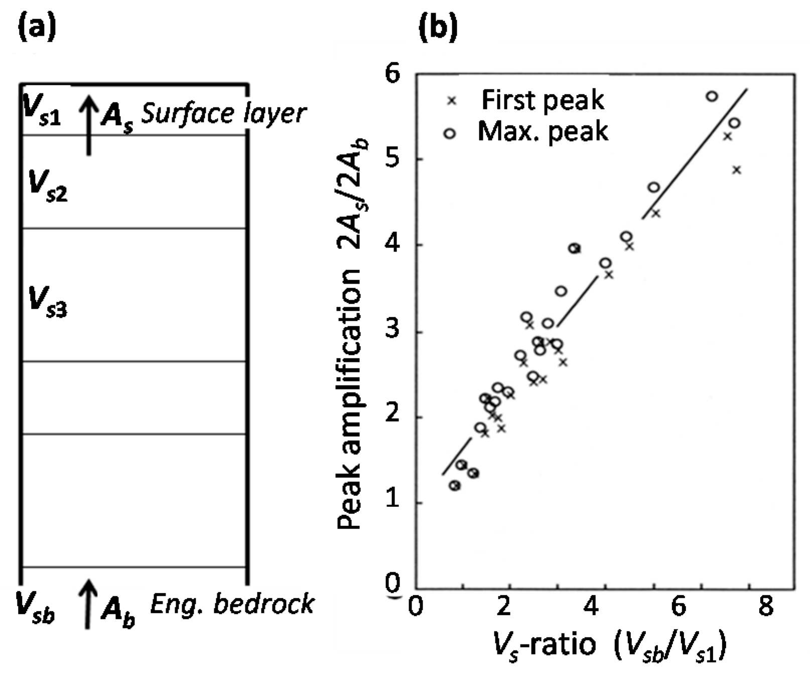
Shima [3] in 1978 showed by conducting a simple one-dimensional wave propagation analysis that the site amplification of SH wave is almost uniquely related to the ratio of S-wave velocities V_s (a base layer to a top layer) irrespective of soil layers in between. As indicated in Figure 1, the spectrum peak amplifications between top and base were almost linearly correlated with the corresponding V_s-ratios (b) in many site conditions analyzed with various V_s-profiles (a).

This finding further implies that amplification at a site relative to another may be evaluated from the ratios of the top layer V_s at the two sites if they share the common base layer of identical V_s-value. This seems to be compatible with a basic concept in currently employed formulas using near-surface S-wave velocities in the seismic zonation. However, a V_s-value not necessarily of the top surface layer but an average V_s-value of multiple layers to a certain depth is chosen in practice, because a surface layer is sometimes too thin to represent a site properly.

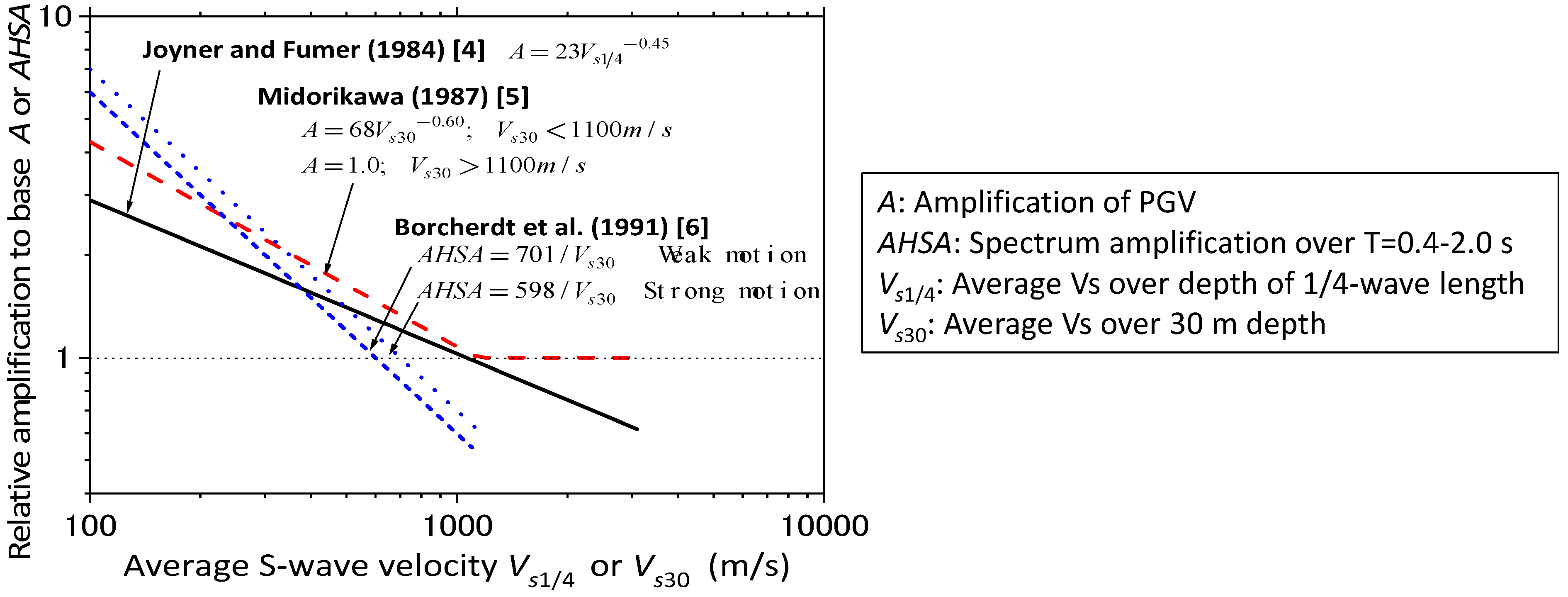
Thus, a couple of empirical formulas were proposed using V_s-values near the ground surface, as summarized in Figure 2. The empirical formula by Joyner and Fumal (1984) [4] evaluates maximum surface acceleration (PGA), maximum velocity (PGV) or 5% damping response spectrum using average V_s in surface layers based on strong motion data obtained in the United States. Here, the V_s-value is averaged over the soil thickness corresponding to a 1/4-wavelength from the ground surface, assuming seismic motions with the predominant period of T = 1.0 s. Another empirical formula was proposed by Midorikawa (1987) [5] based on earthquake records in Japan, wherein the ratio of maximum velocity amplitudes between ground surface and the base was correlated with the S-wave velocity averaged over surface top 30 m, V_s30 (m/s). A similar empirical formula was also proposed by Borcherdt et al. (1991) [6] in the US incorporated records during the 1989 Loma Prieta earthquake in California and associated small shocks, wherein the spectrum amplifications averaged over the period T = 0.4–2.0 s, were correlated with the top 30 m S-wave velocity V_s30 (m/s). Thus, there have been a couple of site amplification evaluation methods currently used in seismic zonation practice.

More recently, the world has experienced quite a few destructive earthquakes. Most have been recorded at the ground surface of different geologies, including outcropping engineering bedrock as horizontal array records (e.g., BSSC 2003 [7]). In addition, vertical array earthquake observation systems have been increasingly deployed, particularly in Japan, wherein site-specific amplifications can be investigated at the same sites along with the depth, having various geological profiles between the ground surface and downhole base. Among them, a number of vertical arrays named KiK-net have been systematically deployed at more than 700 sites all over Japan after the 1995 Kobe earthquake by NIED (National Research Institute for Earth Science and Disaster Resilience in Tsukuba, JAPAN). Each KiK-net recording site consists of a pair of three-dimensional accelerometers (EW, NS, UD), one at the ground surface and another downhole deeper than engineering bedrock, enabling to measure the site amplification between the two [8]. It is generally accepted that the engineering bedrock can serve as a common scale to define relative site amplification among sites sharing the same bedrock, though deeper geological structures may have some effect on absolute amplification (e.g., Trifunac 1990 [9]).

A factor potentially influencing the site amplification during nearfield destructive earthquakes may be the nonlinearity of soil properties in soft soil sites. During the 1964 Niigata earthquake in Japan, acceleration records showed extraordinary low-amplitude long-period motions (Kanai 1966 [10]), presumably reflecting the base-isolation of intensively liquefied ground. During the 1995 Kobe earthquake, Port Island vertical array recorded evident de-amplification of horizontal acceleration due to extensive liquefaction of reclaimed soils (Kokusho & Matsumoto 1998 [11]). Thus, the soil nonlinearity effect has been recognized to be considerable during strong earthquakes. There have been several studies to investigate the soil nonlinearity effect by utilizing KiK-net records of strong and weak motions (e.g., Kokusho & Sato 2008 [12], Kokusho 2013 [13], Régnier et al., 2013 [14]), though it is not clearly taken into account in a hazard map or seismic zonation due to absence of sufficient observational evidence.

In the present paper, eight strong earthquakes in 2000–2008 recorded at many KiK-net vertical array stations throughout Japan are addressed to investigate how their spectrum peak amplifications between surface and engineering bedrock are correlated with the soil profiles and associated V_s there. In preparing for that, how to properly make use of the vertical array data in conducting the amplification study is first discussed. Then, empirical relationships between the amplification and V_s-ratios are explored by incorporating a number of vertical array records of mainshocks during the eight earthquakes. Finally, strain-dependent soil nonlinearity effect on the amplification is investigated by combining mainshocks and aftershocks recorded at the same sites, and an intriguing result obtained there will be examined in a simple theoretical study to find a global picture of soil nonlinearity effect on site amplification.

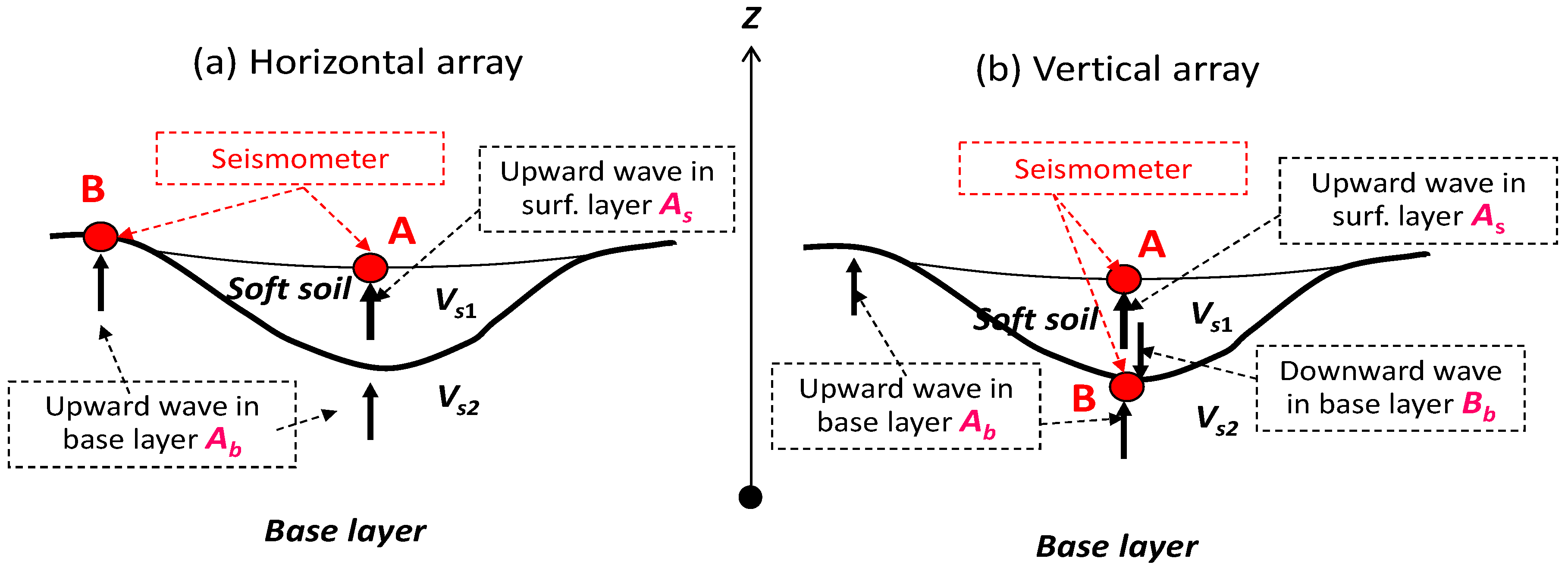
2. Vertical Array Compared to Horizontal Array

In general, there can be two different array systems to measure the earthquake amplification at a site between the ground surface and base layer as illustrated in Figure 3.

(a)

Surface array consisting of a set of surface seismometers on different locations with different surface geologies in a limited distance, sharing a common base layer preferably. Seismic records with the amplitude 2A_s on a surface soil and 2A_b on outcropping base layer, where A_s and A_b are amplitudes of upward waves, $A_s\left(\omega \right)e^{i\omega \left(t-z/V_{s1}\right)}$ and $A_b\left(\omega \right)e^{i\omega \left(t-z/V_{s2}\right)}$ in the soft soil and stiff base layer respectively, as a function of angular frequency $\omega$ but abbreviated here, travelling toward positive z-direction with S-wave velocity V_s1 and V_s2, as indicated in Figure 3. The site amplification between the two different geologies can be directly evaluated 2A_s/2A_b if upward wave amplitude A_b in base is assumed to be basically unchanged in the area. This amplification 2A_s/2A_b is what we need to develop a seismic hazard map for seismic zonation.

(b)

Vertical array consisting of a surface and down-hole seismometers at the same place with exactly the same bedrock upward wave A_b. This can evaluate site amplification at exactly the same location but does not directly provide the amplification 2A_s/2A_b but another value 2A_s/(A_b + B_b) because the downhole record is more or less contaminated by the downward wave B_b from the overlying layers (e.g., Schnabel et al., 1972 [15], Kokusho 2017 [16]). Here, B_b are amplitudes of downward waves $B_b\left(\omega \right)e^{i\omega \left(t+z/V_{s1}\right)}$ in the soft soil layer. Hence, modification of 2A_s/(A_b + B_b) in the vertical array is necessary to evaluate the amplification 2A_s/2A_b for seismic zonation. In conducting the modification, it is required to pay attention to another important feature of the vertical array different from the horizontal array as described below.

Figure 4a–f show typical examples of the theoretical transfer function 2A_s/(A_b + B_b) (thick dashed curves) compared with the corresponding 2A_s/2A_b (thick solid curves) calculated from soil profile data in six vertical array sites during two earthquakes (EQ3 and EQ5) of KiK-net database summarized in

Table 1. 8 strong earthquakes EQ1~EQ8 recorded by KiK-net vertical arrays and utilized in this paper with pertinent values.

EQ No.	Name of EQ	Year	Moment Mag. Mw	JMA Mag. MJ	PGA of MS Addressed (g)	No. of Sites & MS Records Addressed	No. of Sites/MS Analyzed in This Paper	No. of Sites/AS Analyzed in This Paper	PGA of MS Analyzed (g)	PGA of AS Analyzed (g)
EQ1	Tottoriken-Seibu	2000	6.8	7.3	>0.1	18	4/4	4/16	0.24–0.13	0.0028–0.0298
EQ2	Geiyo	2001	6.7–6.8	6.4	>0.1	17	3/3	3/12	0.34–0.23	0.0026–0.0237
EQ3	Tokachi-Oki	2003	7.9	8.0	>0.2	20	9/9	6/24	0.58–0.24	0.0017–0.0198
EQ4	Niigataken-Chuetsu	2004	6.6	6.8	>0.1	15	9/9	6/24	0.59–0.11	0.0014–0.1253
EQ5	Fukuokaken Seiho-Oki	2005	6.7	7.0	>0.1	11	2/2	0/0	0.25–0.20
EQ6	Noto-Hanto	2007	6.7	6.9	>0.05	10	6/6	4/16	0.11–0.03	0.0019–0.0197
EQ7	Niigataken-Chuetsu-Oki	2007	6.6	6.8	>0.1	10	4/4	4/16	0.26–0.11	0.0013–0.0800
EQ8	Iwate-Miyagi Nairiku	2008	6.9	7.2	>0.15	17	2/2	1/4	2.45–0.16	0.0078–0.0125
Total						118	39/39	28/112

. The installation levels of surface and downhole seismometers are indicated with the pair of arrows in site profiles. The V_s-profiles (included in the figure) obtained by in situ S-wave logging are available in the KiK-net vertical array database. The two thin curves also overlaid in the charts represent observed Fourier spectrum ratios (the ratio of Fourier spectrums of observed motions between surface and downhole) in EW and NS directions for earthquake records obtained there. At all the sites, peak frequencies of 2A_s/(A_b + B_b) are mostly compatible with those of observed spectra in lower frequency peaks at least, indicating practical applicability of one-dimensional soil models in these sites to a certain extent.

Then, if the transfer function 2A_s/(A_b + B_b) is compared with 2A_s/2A_b, the correspondence in peak frequency is perfect in (a) and good in (b) despite the peak heights are distinctively higher in the former than the latter because of different contribution of radiation damping as mentioned later. The correspondence seems to be still tolerable in (c). However, it gets poorer in (d) and very poor in (e) and (f) because the spectrum 2A_s/2A_b tends to deform quite differently from 2A_s/(A_b + B_b).

The reason may be given by examining the soil profiles. In (a) and (b), the V_s-value at the base is much larger than the upper layers, and the depth of the downhole seismometer is not so deep from the boundary of clear V_s-contrast indicated by a triangle. In (c) and (d), the V_s-value at the base layer is not so much varied from that in the upper layer, and the seismometer depth is getting deeper from the boundary of V_s-contrast again. In (e) and (f), though V_s at the base layer is much greater than the upper layers, the depth of the seismometer is too deep from the boundary of clear V_s-contrast to properly detect the response of the upper layers. This observation tells us the importance of appropriate in-advance planning in deploying a vertical array system considering site-specific soil profiles.

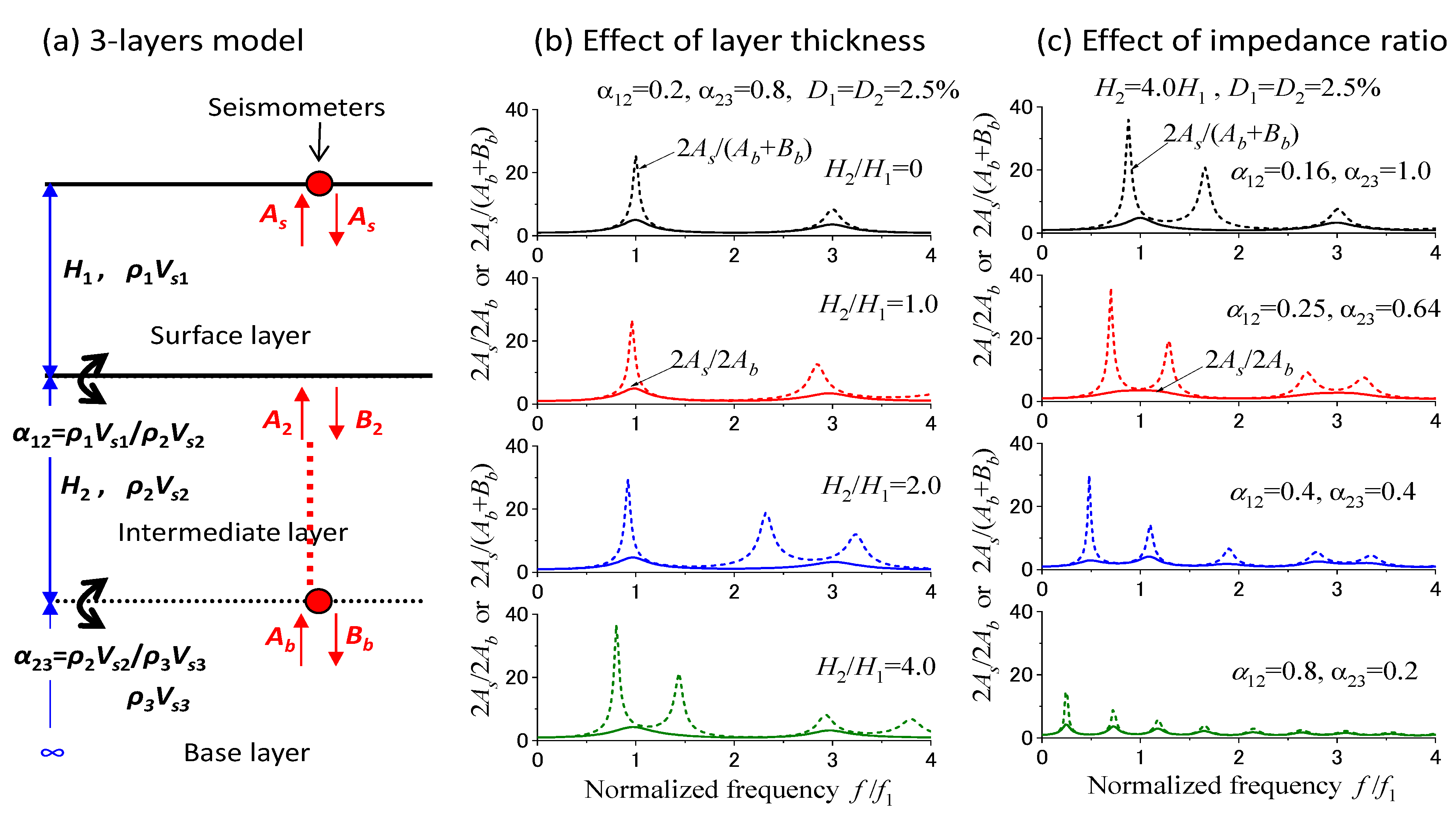
In order to clarify a basic principle of how peak frequencies in 2A_s/(A_b + B_b) and 2A_s/2A_b are governed by soil profiles, a simple one-dimensional three-layer model as shown in Figure 5a has been analyzed. An arbitrary in situ soil profile may be simplified by the model consisting of a soft surface layer (first layer: thickness H₁), an intermediate layer (second layer: H₂), and a stiff base layer (third layer) with infinite thickness. Wave amplitudes are A_s, A₂, A_b upward and A_s B₂, B_b downward, at the surface, intermediate, and base layers, respectively. The impedance ratios are ${\alpha }_{12}$ = ${{\left(\rho V_s\right)}_1/\left(\rho V_s\right)}_2$ between the first and second layer, and ${\alpha }_{23}={{\left(\rho V_s\right)}_2/\left(\rho V_s\right)}_3$ between second and third. The down-hole seismometer is positioned at the top of the base layer. The two transfer functions between surface and base, 2A_s/(A_b + B_b) and 2A_s/2A_b, are calculated for the model and shown in (b) and (c) against the normalized frequency f/f₁ where f₁ = Vs₁/(4H₁).

In (b) where the thickness of intermediate layer H₂ is parametrically varied with respect to H₁ while keeping ${\alpha }_{12}$ = 0.2 and ${\alpha }_{23}$ = 0.8, the transfer function 2A_s/2A_b (solid curve) is very consistent with its stable peak frequency $f/f_1\approx 1.0$ irrespective of the H₂/H₁-ratio because of the clear impedance contrast ${\alpha }_{12}$ = 0.2 between the surface and intermediate layer. In contrast, the shapes and peak frequencies of the transfer function 2A_s/(A_b + B_b) (dashed curve) tend to change obviously with increasing H₂/H₁-ratio for H₂/H₁ ≥ 2.0 in particular. This is because, in 2A_s/(A_b + B_b), the depth of seismometer installation works as a virtual rigid boundary with no wave energy radiation into the underlying layer even if it is in the midst of a uniform layer according to a simple multi-reflection theory of SH-wave (e.g., Schnabel et al., 1972 [15], Kokusho 2017 [16]).

In (c), where the impedance ratios ${\alpha }_{12}$, ${\alpha }_{23}$ are parametrically changing (keeping ${\alpha }_{12}\times {\alpha }_{23}$ = 0.16 constant) with a constant thickness ratio H₂/H₁ = 4.0, 2A_s/(A_b + B_b) and 2A_s/2A_b are quite different in peak frequencies for ${\alpha }_{23}$ ≈ 0.64 or larger, though they coincide to each other if ${\alpha }_{23}$ ≈ 0.4 or smaller. This indicates that a sharp impedance contrast is preferable at the base boundary near the down-hole seismometer for better matching between the two transfer functions.

Consequently, in deploying vertical array systems, the downhole seismometers should be installed with enough care in a stiff base layer not too deep from the layer boundary. The clearer the impedance contrast at the base boundary to the overlying layer, the better matching in peak frequencies is possible. If the depth of the down-hole seismometer is twice or further deeper than the surface layer thickness, H₂/H₁ > 2.0, from the boundary of major impedance contrast, virtual peaks with quite different frequencies from those in 2A_s/2A_b tend to appear in 2A_s/(A_b + B_b) for vertical arrays unless the impedance contrast is clear enough. Thus, there should be an appropriate installation depth for the down-hole seismometer closely dependent on individual site conditions. It is never the deeper, the better. The installation depth of down-hole seismometers may sometimes be predetermined by the economy or other specifications. In the case of KiK-net, too, due care was necessary to tackle this problem, and only appropriate data have been chosen in this research for the amplification analysis as explained below.

3. Earthquake Records and Soil Profiles

KiK-net records corresponding to 8 earthquakes (EQ1 to EQ8) utilized in this paper are listed in Table 1. The moment magnitudes M_w listed together with M_J (Japan Meteorological Agency magnitude) are varied from 6.6 to 7.9. A total of 118 mainshocks (MS) records during the eight earthquakes observed in vertical array sites near focal areas were firstly addressed. As shown in Figure 6a, the PGA-values in the vertical axis are spanning from 0.4 to 2.5 g, while maximum accelerations at the base are 0.01–1.0 g, leading to approximately 2–16 times amplification in maximum horizontal acceleration in terms of 2A_s/(A_b + B_b) between surface and base. Among them, those with filled symbols have been selected for the amplification analysis later on.

The depths of the down-hole seismometers in the vertical arrays addressed here vary mostly from 100 m to 330 m. S-wave velocities in the top and bottom of all the vertical arrays are plotted in the vertical and horizontal axes, respectively, in Figure 6b. The bottom velocities V_sb in many earthquake recording sites diverge from 400 m/s to 3000 m/s, though all of them are stiff enough to be considered as the engineering bedrock while some are approaching seismological bedrock corresponding to the earth crust of hard rock with a high density $\rho \ge$ 2.7 t/m³ and high S-wave velocity V_s ≥ 3000 m/s. In a good contrast, the majority of surface velocities V_s in most of the sites are within a limited extent; about 100 to 400 m/s, around 200 m/s on average. Among the plots, those of filled symbols have been selected for the later analysis.

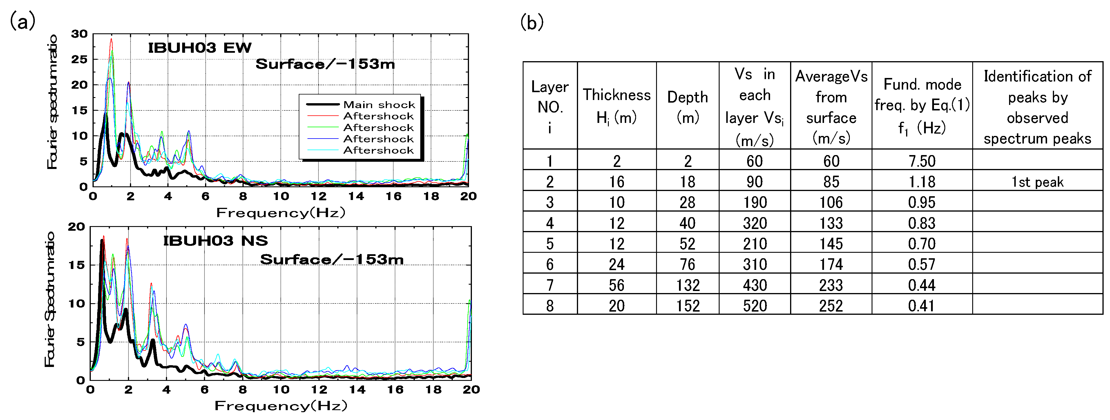
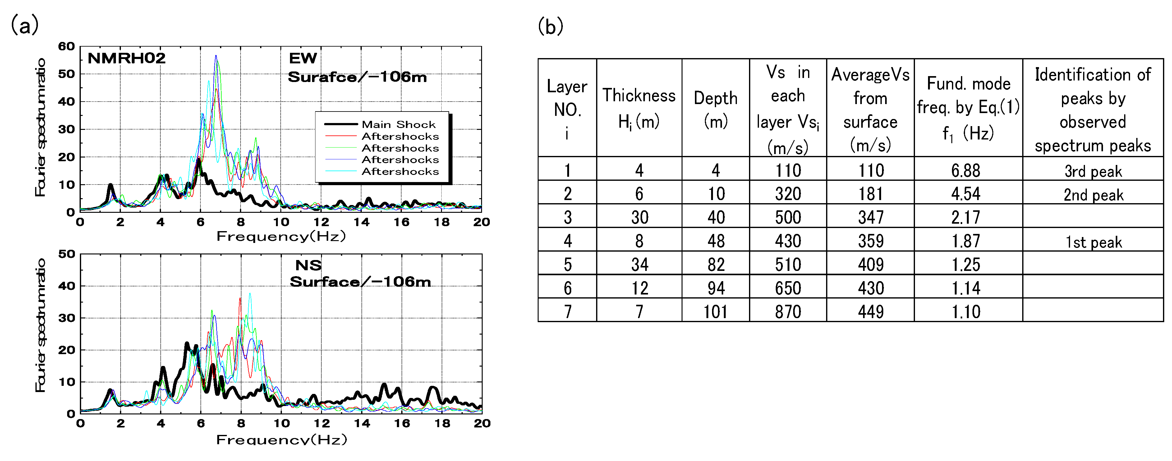
Fourier spectrum ratio 2A_s/(A_b + B_b) between surface and base is calculated using the surface and downhole records in each KiK-net vertical array site. A typical result in EW and NS direction for the mainshock and several aftershocks at a site during EQ3 is shown together with associated soil profile data in Figure 7a,b. A similar result at another site during EQ3 is shown in Figure 8a,b. The aftershocks (AS) were chosen among the KiK-net dataset to have distinctively low PGAs and hypocenters not far compared to the mainshock (MS) as indicated in Table 1. It is noted in Figure 7 and Figure 8 that the spectrum peak frequencies are almost matching among multiple aftershocks in EW/NS directions in the lower frequency peaks, at least in these two sites. Also noticed is a clear difference in the amplitude and peak frequency of the spectrum ratios between the mainshock and aftershocks. It presumably reflects strain-dependent nonlinear soil properties during strong shaking, which appears to be more pronounced in higher-order peaks due to the larger involvement of shallower layers.

4. S-Wave Velocity Ratio versus Site Amplification

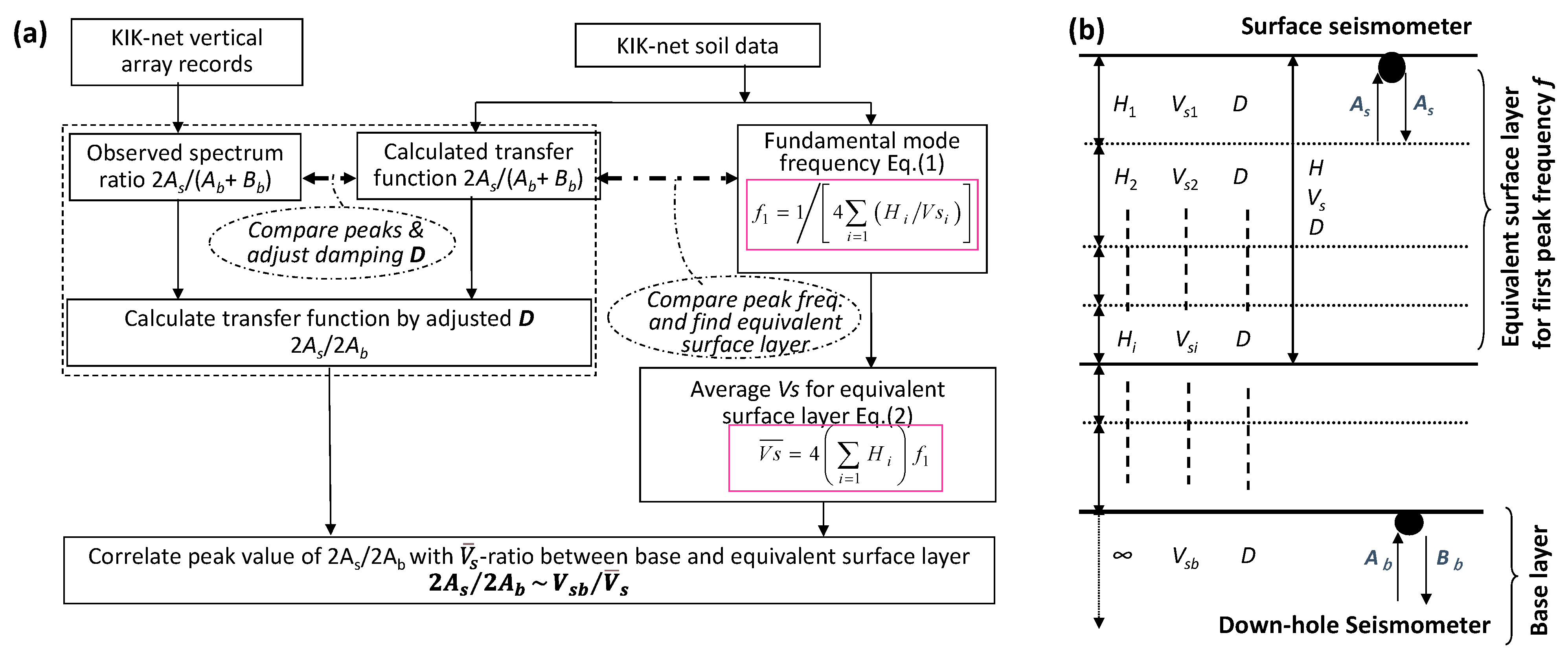
A flow chart is illustrated in Figure 9a to develop a reliable correlation between site amplification and S-wave velocity based on the vertical array database in this research. Totally 39 mainshock records have been selected out of 118 during eight earthquakes initially addressed as listed in Table 1. The following two criteria was employed in the selection to reduce various potential errors involved during the data reduction process.

(1)

Similarity of transfer functions between 2A_s/(A_b + B_b) and 2A_s/2A_b calculated by the soil model in terms of peak frequencies as already discussed in Figure 4. Among the six charts in Figure 4; for example, (a) to (c) are acceptable because the first peak frequency (the lowest peak frequency) at least is coincidental in contrast to very displaced peaks in (d) to (f).

(2)

The similarity of the first peak frequency in 2A_s/(A_b + B_b) between the observed spectrum ratio and the computed transfer function so that the soil model is reliable enough.

Here, the acceptable relative difference in peak frequencies was regulated within 1/1.5 to 1.5 between the two functions.

Then, fundamental mode frequencies f of the layered soil system were calculated by a 1/4-wavelength formula, Equation (1), in order to specify equivalent soil layers generating peak frequencies in the spectrum ratio, based on the soil profile together with the S-wave velocities of individual layers provided by the KiK-net database.

$$f=1/\left[4\sum _{i=1}^n\left(H_i/V_s{}_i\right)\right]$$

(1)

Here, as depicted in Figure 9b, H_i and V_si are the thickness and S-wave velocity of the i-th layer sequentially numbered from the top, and H_i/V_si is summed up layer by layer down to the base. This is an extension of the well-known 1/4 wavelength formula in a two-layer system for roughly determining predominant frequency in a multi-layer system based on the same principle of first resonance. The calculated frequency is compared one by one with the peak frequencies in the observed spectrum ratio such as in Figure 7a or Figure 8a to identify equivalent surface layers of thickness $H={\displaystyle \sum H_i}$ consisting of one or more layers generating the fundamental mode frequencies calculated by Equation (1) as tabulated in Figure 7b or Figure 8b.

In Figure 10a, the first peak frequencies f calculated by Equation (1) based on given soil data are plotted with solid symbols in the horizontal axis versus the frequencies f* identified in the observed spectrum ratios (EW and NS directions) in the vertical axis for the selected 39 mainshock records of eight earthquakes. There exists a satisfactory correspondence between f based on Equation (1) and the peak frequency f* observed in spectrum ratios where almost all plots are within f* = 0.8 f and f* = 1.2 f. In the same figure, f in Equation (1) is also compared with first peak frequencies of the transfer functions 2A_s/(A_b + B_b) and 2A_s/2A_b, respectively, computed by the 1D soil model based on the KiK-net soil profile data. Though some plots are dispersed beyond the lines f* = 0.8–1.2 f, the difference is well within 1/1.5–1.5 times as initially regulated. Then, the average S-wave velocity $\overline{V_s}$ for the equivalent surface layer is determined by Equation (2) from the fundamental mode frequency f identified as the first peak and its thickness $H={\displaystyle \sum H_i}$.

$$\overline{V_s}=4Hf$$

(2)

In Figure 10b, $\overline{V_s}$-values (m/s) thus determined from the first peak frequencies are compared with V_s30 (m/s), S-wave velocities averaged over the top 30 m from ground surface often used in current practice, which is calculated by the next equation Equation (3) where $T_{30}$(s) is the time of S-wave propagation for the top 30 m based on V_s-logging data. It indicates that $\overline{V_s}$-value introduced in this research is positively and loosely correlated with V_s30.

$$V_s{}_{30}=30/T_{30}$$

(3)

The next step after determining the average S-wave velocity of the equivalent surface layer generating the peak frequency is how to evaluate 2A_s/2A_b from 2A_s/(A_b + B_b) as illustrated in the flowchart (Figure 9a) and described below.

(1)

A theoretical transfer function, 2A_s/(A_b + B_b) is calculated based on a soil model in each site using the given soil/V_s-profile with frequency-independent damping ratio, D, tentatively assumed as 2.5% throughout the layer.

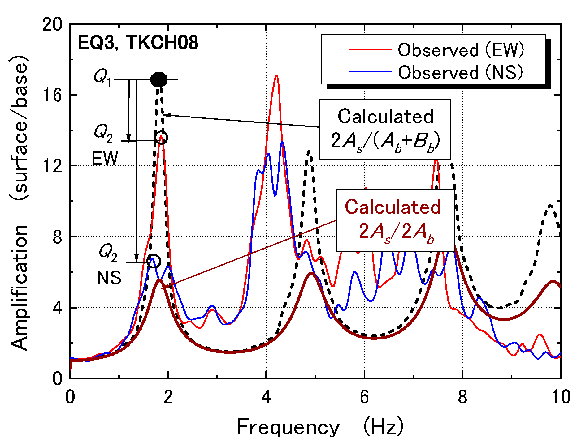
(2)

The function 2A_s/(A_b + B_b) is compared with the spectrum ratio of observed records, as exemplified in Figure 11. If a peak frequency in the transfer function can be found within the allowable difference in the spectrum ratio of observed motions, it is identified as the corresponding peak, and the damping ratio assumed as D = 2.5% previously is modified uniformly by D = Q₁/Q₂ × 2.5% to have the identical peak value, where Q₁ is the peak amplitude of the transfer function, and Q₂ is that of spectrum ratio of the observed records.

(3)

Another theoretical transfer function 2A_s/2A_b is computed using the modified damping ratio D (averaged between EW and NS directions) based on the same soil model, and the peak value is read off as the peak amplification for the corresponding horizontal array as also indicated in Figure 11.

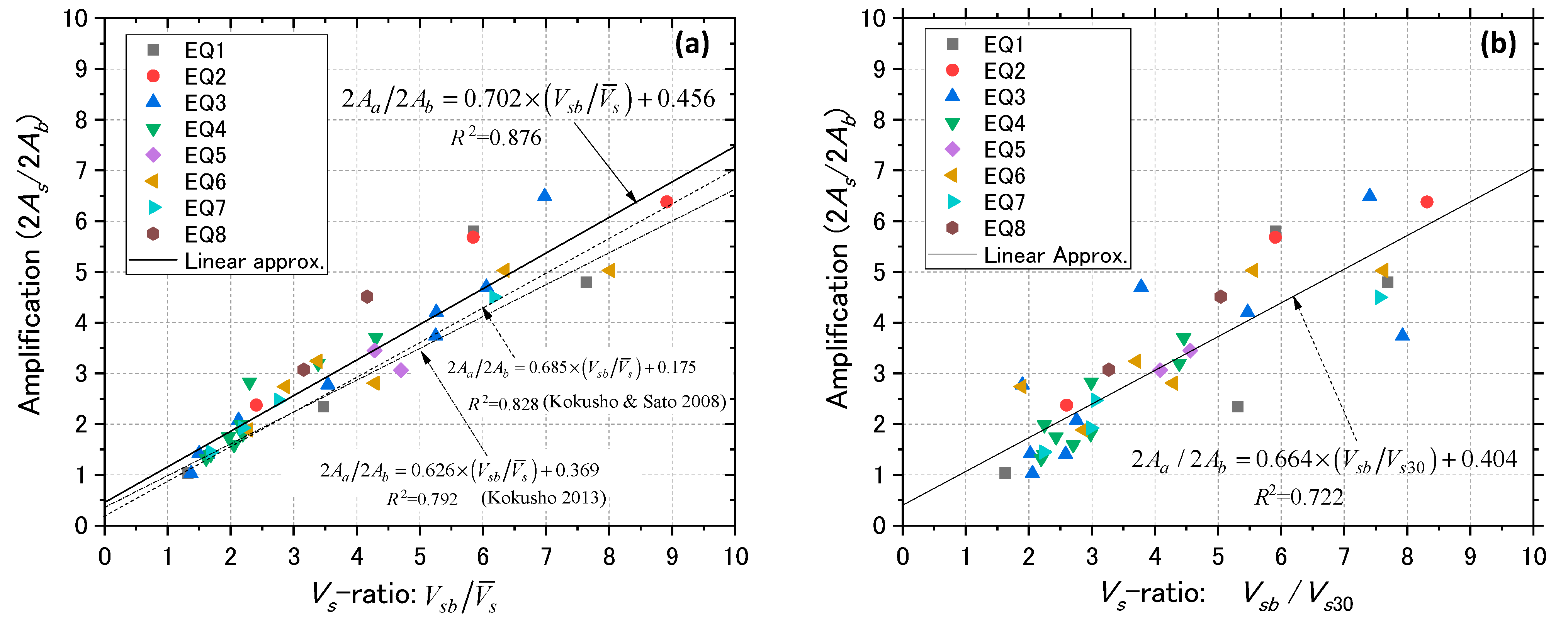
Figure 12a shows the peak amplitudes of 2A_s/2A_b thus determined and plotted in the vertical axis versus the $\overline{V_s}$-ratio in the horizontal axis for 39 mainshock records of the eight strong earthquakes. The $\overline{V_s}$-ratio, $V_s{}_b/\overline{V_s}$, is defined here as the S-wave velocity at a base layer $V_s{}_b$ divided by the velocity $\overline{V_s}$ evaluated by Equation (2) for the first peak frequency based on V_s-profiles at each site. The $\overline{V_s}$-ratio correlate fairly well with 2A_s/2A_b all through the eight earthquakes recorded at various sites. It may be approximated by the next linear equation with the determination coefficient R² = 0.876 as superposed with a solid straight line on the chart.

$$2A_a/2A_b=0.702\times \left(V_{sb}/{\overline{V}}_s\right)+0.456$$

(4)

In previous research conducted by the present author (Kokusho and Sato 2008 [13]), wherein out of the same KiK-net vertical array data, those belonging to EQ3, EQ4, EQ 5 were analyzed, the correlation $2A_a/2A_b=0.685\times \left(V_{sb}/{\overline{V}}_s\right)+0.175$ (R² = 0.828) was obtained. Another previous research (Kokusho 2013 [14]), where the same KiK-net data of 8 earthquakes was utilized, $2A_a/2A_b=0.626\times \left(V_{sb}/{\overline{V}}_s\right)+0.369$ (R² = 0.792) was yielded. In these previous papers, unlike this paper the strict data selection with regard to peak frequency correspondence between 2A_s/2A_b and 2A_s/(A_b + B_b) using the criteria already mentioned, was not implemented. Furthermore, not only the first peak but also higher-order peaks were also analyzed in a similar manner. The correlation obtained here seems quite reasonably better than the previous ones with higher R²-values, though the previous correlations superposed in Figure 12a with thin lines are not so much different.

In Figure 12b, the same peak values in 2A_s/2A_b are plotted versus velocity ratio, V_sb/V_s30. It is approximated by the next equation with R² = 0.722, wherein the plots are evidently more scattered than in Figure 12a. This indicates that the S-wave velocity of the top 30-m V_s30 may somehow evaluate the site amplification to a certain extent despite that the effect of site-specific soil-profiling is ignored.

$$2A_a/2A_b=0.664\times \left(V_{sb}/V_{s30}\right)+0.404$$

(5)

Thus, the site amplification for zonation study relative to an outcropping base layer has been formulated for first spectrum peaks corresponding to the predominant frequency in situ, of many vertical array sites during eight strong earthquakes as either Equations (4) or (5). The former may be recommended because of the larger R²-value for higher accuracy in predicting the site amplification, though both formulas may be useful practically. It should be noted that they may be applicable to arbitrary engineering bedrock with various V_sb and depth because they have been developed from soil profiles including a wide variety of base layers with $V_s{}_b$ = 400 m/s to 3000 m/s as indicated in Figure 6b.

With respect to Equation (4), site amplification may be readily assessed by the aid of microtremor measurements, even if no information on soil profiles is available, as

(1)

Decide predominant frequency f of a site using H/V spectrum ratios calculated from Horizontal and Vertical microtremor records (Nakamura 1989 [17]).

(2)

Estimate the thickness H of soft soil or equivalent surface layer where the predominant frequency is exerted, which is sometimes possible based on geological maps or high-density soil logging data available in city areas.

(3)

Then, the average S-wave velocity in the equivalent surface layer where the predominant frequency is exerted can be calculated by $\overline{V_s}=4Hf$.

(4)

Calculate the S-wave velocity ratio $V_s{}_b/\overline{V_s}$ from $V_s{}_b$ of a base layer, which can be normally given by geological database of the area.

(5)

Equation (4) using the $V_s{}_b/\overline{V_s}$-value will give the site amplification with respect to the common base layer. The relative amplification at two sites sharing the same base layer can be obtained by directly comparing them. If different base layers are chosen in two sites, the relative amplification can still be readily adjustable in Equation (4) by considering the difference in V_sb. The same procedures can also be followed when Equation (5) for V_sb/V_s30 is used in place of Equation (4) for $V_s{}_b/\overline{V_s}$.

5. Soil Nonlinearity Effect

In order to investigate the effect of soil nonlinearity on the site amplification using actual earthquake data, aftershock records were compared with corresponding mainshock records in the same sites. For the comparison, 28 recording sites were selected, as summarized in Table 1 out of 39 where mainshocks were analyzed. Four aftershocks were chosen in individual sites (112 aftershock records in total) with their PGAs distinctively different, as small as 1% to 10~65% maximum to the mainshocks as summarized in Table 1. The first peak values of 2A_s/2A_b were adjusted in the same way as mainshocks using D-values determined from the peaks of 2A_s/(A_b + B_b), and the values in EW and NS directions were averaged.

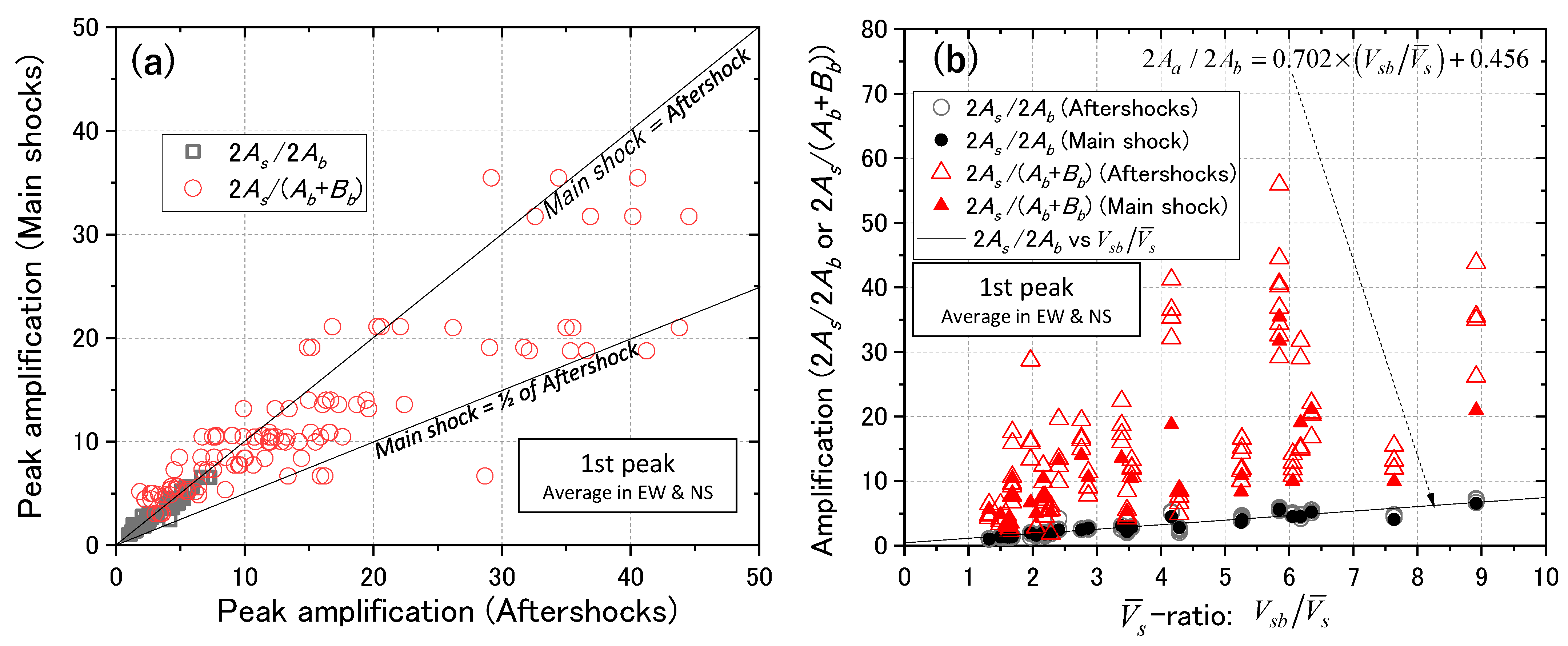
In Figure 13a, the peak spectrum amplification of the first peak of 112 aftershocks are plotted in the horizontal axis versus those of 28 corresponding mainshocks in the vertical axis for 2A_s/2A_b (horizontal array) with open square symbols, and the same for 2A_s/(A_b + B_b) (vertical array) with open circles. It is noted that the absolute amplification values of 2A_s/2A_b are far smaller than 2A_s/(A_b + B_b) mainly because the former is strongly influenced by radiation damping by underlying layers, while the radiation damping is ineffective in the latter. It is also remarkable is that 2A_s/2A_b shows almost identical amplification between MS and AS, while 2A_s/(A_b + B_b) seems to be quite different, wherein the mainshock amplifications can be as low as half of the aftershocks.

In Figure 13b, the same peak spectrum amplifications, 2A_s/(A_b + B_b) and 2A_s/2A_b, are plotted versus $\overline{V_s}$-ratio ($V_s{}_b/\overline{V_s}$) for mainshocks and aftershocks of the 8 earthquakes with filled and open symbols. For 2A_s/2A_b, a clear correlation can be recognized between the peak amplification and $\overline{V_s}$-ratio, which can be approximated by Equation (4), again. It should also be noted that the difference in peak amplifications between the mainshock and corresponding aftershocks are really marginal, indicating a negligible effect of soil-nonlinearity. In contrast, the plots for 2A_s/(A_b + B_b) are not so well correlated to $\overline{V_s}$-ratio. Furthermore, the peak amplifications of 2A_s/(A_b + B_b) for the mainshocks (filled triangles) are evidently smaller than the corresponding aftershocks (open triangles) in most sites. This indicates that the soil nonlinearity effect is evidently seen in vertical array earthquake records but far less pronounced in surface array records. The soil nonlinearity effect was also clearly recognized independently by Régnier et al. (2013), where the borehole site response corresponding to 2A_s/(A_b + B_b) was investigated using KiK-net vertical array records, though outcrop site response 2A_s/2A_b was not addressed in the same study.

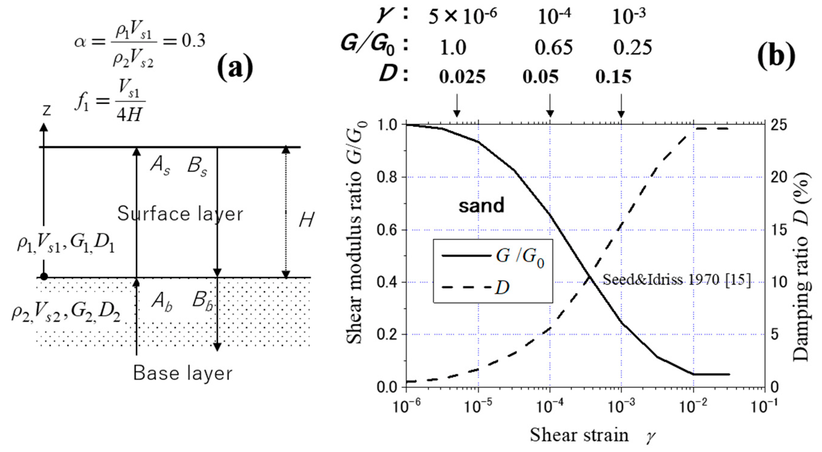
In order to account for these widely different soil nonlinear effects in the two earthquake recording arrays, a simple two-layer system of a surface layer (Impedance = ${\rho }_1{V}_s{}_1$, Shear modulus G₁ = ${\rho }_1{V}_s{{}_1}^2$, Damping ratio = D₁) underlain by an infinitely thick base layer (Impedance = ${\rho }_2{V}_s{}_2$, Shear modulus G₂ = ${\rho }_2{V}_s{{}_2}^2$, Damping ratio = D₂) shown in Figure 14a was studied, assuming the impedance ratio for small strain properties as $\alpha ={\rho }_1{V}_s{}_1/{\rho }_2{V}_s{}_2$ = 0.3. The transfer functions 2A_s/(A_b + B_b) and 2A_s/2A_b can be expressed by Equations (6) and (7), respectively [12];

$$2A_s/\left(A_b+B_b\right)=2/\left(e^{i{k}_1{}^{*}H}+e^{-i{k}_1{}^{*}H}\right)$$

(6)

$$2A_s/2A_b=2/\left[\left(1+{\alpha }^{*}\right)e^{i{k}_1{}^{*}H}+\left(1-{\alpha }^{*}\right)e^{-i{k}_1{}^{*}H}\right]$$

(7)

where $k_1{}^{*}=\omega /\left(V_{s1}\sqrt{1+2i{D}_1}\right)$ and ${\alpha }^{*}=\alpha \sqrt{\left(1+2i{D}_1\right)/\left(1+2i{D}_2\right)}$.

In taking into account the effect of strain-dependent soil properties on the amplification, the shear modulus degradation G/G₀ from small-strain shear modulus G₀, and the damping ratio D in the surface layer are parametrically changed; G/G₀ = 1.0, 0.65, 0.25 and D₁ = 2.5, 5 and 15%, for strain level of 5 $\times$ 10⁻⁶, 1 $\times$ 10⁻⁴, 1 $\times$ 10⁻³, respectively, assuming a typical degradation curve for sand (Seed & Idriss 1970 [18]) as indicated in Figure 14b, while in the base layer 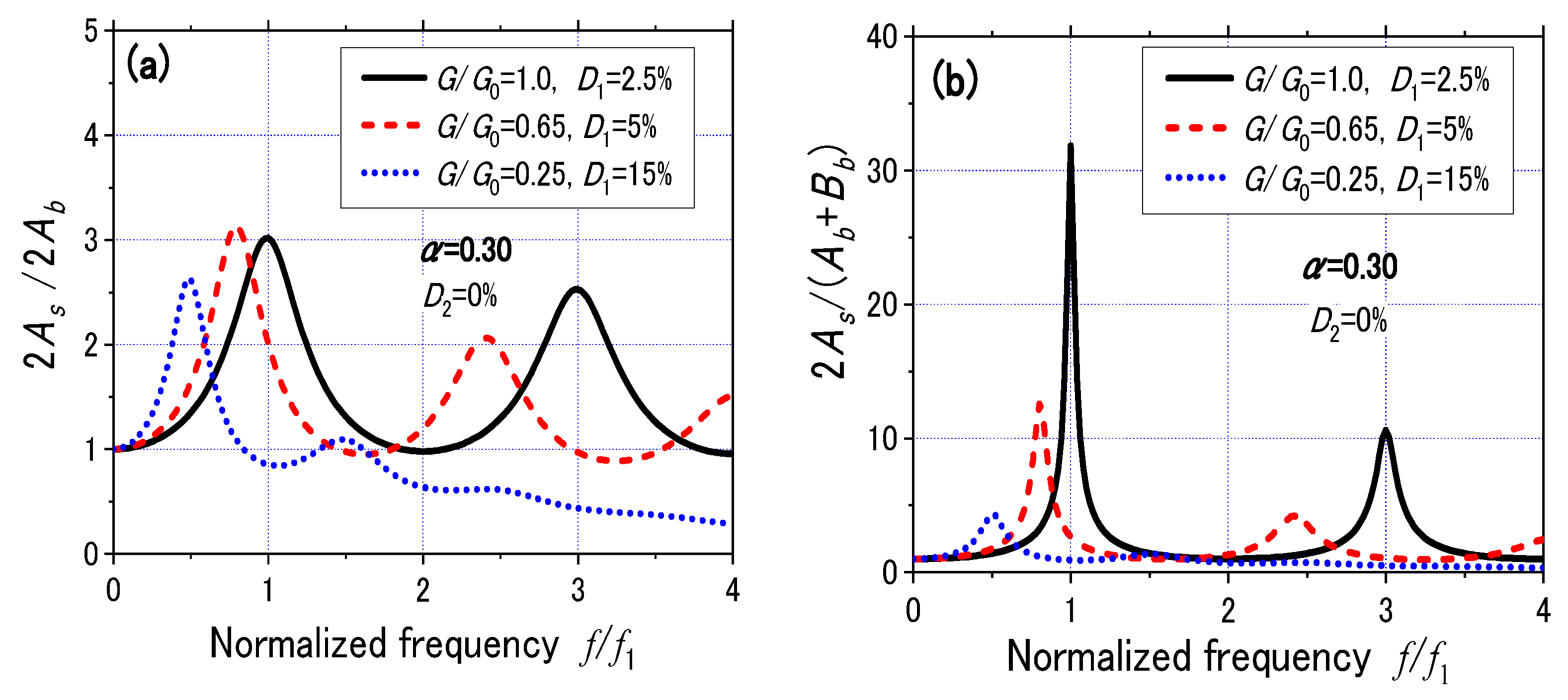D₂ = 0. The calculated results of 2A_s/(A_b + B_b) and 2A_s/2A_b are shown in Figure 15a,b, respectively. Here, the amplification between surface and base is shown versus the normalized frequency, f/f₁, where f₁ = first mode frequency of the surface layer for small strain properties (G/G₀ = 1.0).

Obviously, nonlinear soil properties have a great effect on peak frequency and amplification. In particular, the peak frequency becomes evidently lower with modulus degradation both in 2A_s/(A_b + B_b) and 2A_s/2A_b. However, with regard to peak amplification, it is noted that the soil nonlinearity has a much smaller effect in 2A_s/2A_b than in 2A_s/(A_b + B_b) for the first peak in particular. This is because radiation damping associated with impedance ratio $\alpha ={\rho }_1{V}_s{}_1/{\rho }_2{V}_s{}_2$ tends to dominate 2A_s/2A_b overwhelming the soil nonlinearity effect. In Equation (7), the amplification is expressed as $\left|2A_s/2A_b\right|\approx \left|1/{\alpha }^{*}\right|$ when $k_1{}^{*}\approx \pi /2H$ at the first peak, while no effect of impedance ratio ${\alpha }^{*}$ is involved in 2A_s/(A_b + B_b) as indicated in Equation (6). Under the paramount effect of radiation damping, the difference in the amplification due to strain-dependent properties becomes obscure in 2A_s/2A_b. Furthermore, the impedance ratio $\alpha ={\rho }_1{V}_s{}_1/{\rho }_2{V}_s{}_2$, which becomes smaller with degraded shear modulus in the surface layer, tends to give larger amplification, compensating for the increasing effect of internal soil damping during strong earthquakes. Thus, the difference in soil properties between mainshock and aftershocks tends to have less influence on the amplification in 2A_s/2A_b than in 2A_s/(A_b + B_b), as demonstrated in Figure 13 by actual earthquake records.

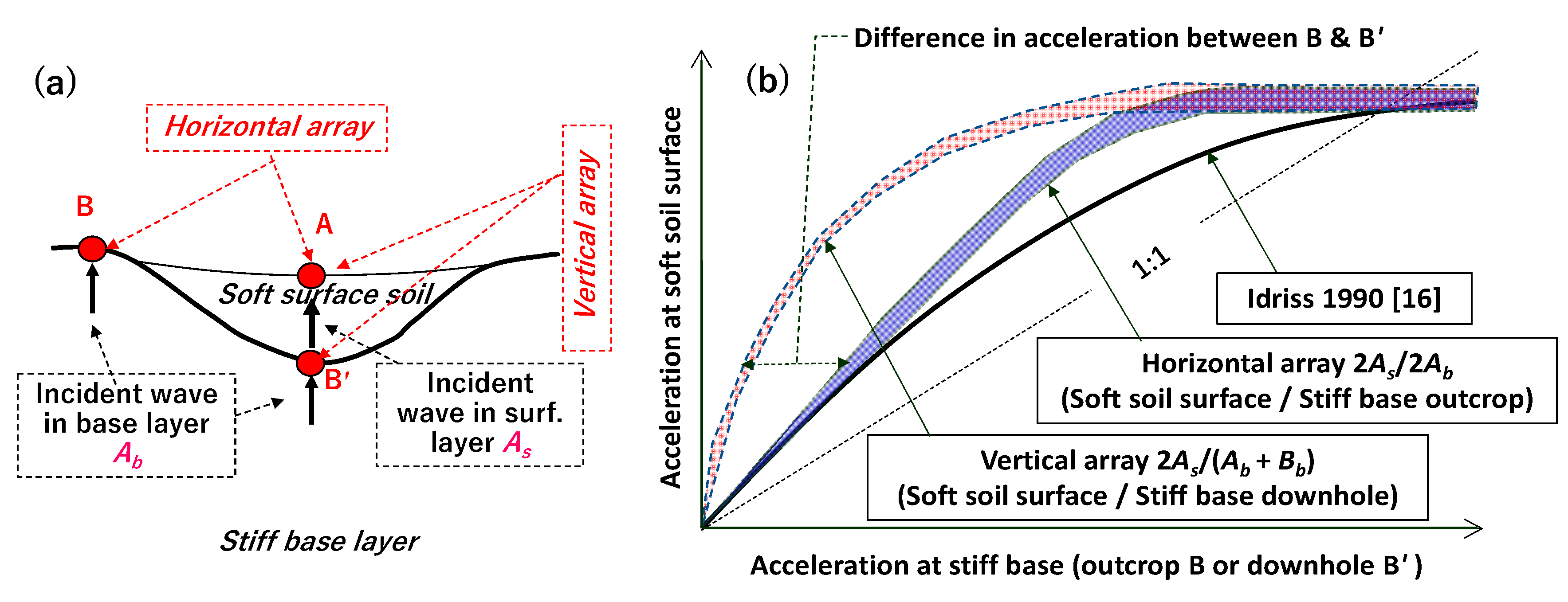
Summarizing the above discussions, there are two definitions of site amplification; the horizontal array and vertical array, as shown here again in Figure 16a, where the horizontal array is directly applicable to the seismic zonation. Figure 16b conceptually shows the accelerations at the stiff base, the point B (outcropping) or B′ (downhole) taken in the horizontal axis versus those at the soil surface, the point A, in the vertical axis. The acceleration on the soft soil surface shows a strong nonlinearity with respect to increasing downhole-based acceleration at B′ due to nonlinear soil properties as schematically illustrated with the dashed shaded belt. In the horizontal array, however, the surface acceleration is remarkably linear with the outcropping base acceleration at B, as illustrated with the solid shaded belt in the same diagram. It has been actually evidenced in Figure 13a that there is no significant amplification difference between mainshock and corresponding aftershocks at many recording sites. This is because the base acceleration in the horizontal axis defined at the outcropping base B tends to be larger than that at the downhole base B′ where the effect of downward waves from the overburdened soils cannot be ignored.

A thick solid curve overlaid in Figure 16b represents a similar relationship of PGA-values at soft soil sites and stiff rock sites proposed in the United States (Idriss 1990 [19]). It was estimated in the framework of the horizontal array from actual smaller earthquake records of similar epicenter distances during the 1985 Mexican earthquake and 1989 Loma Prieta earthquake and from numerical analyses for strong motions as well. The curve is obviously nonlinear, reflecting the soil nonlinearity, and the amplification of soil sites to rock sits to be lower than unity for PGA larger than around 0.4 g, though the PGA and the spectrum peak amplification may possibly be somewhat different in reflecting the soil nonlinearity effect.

The above findings based on the actual records as well as the simple model analysis may indicate that soil nonlinearity is not so pronounced in the horizontal array, unlike the vertical array in terms of spectrum peak amplification, including strong earthquakes. The mainshock records utilized here were with PGA around 0.6 g and even as high as 2.5 g. As for the extreme case of PGA = 2.5 g, no clear difference in the peak amplification of 2A_s/2A_b was observed by one of the plots in Figure 13. The near-surface soil profile there was not so stiff, comprising 2 m thick layer of V_s = 150 m/s underlain by 18 m thick layer of V_s = 430 m/s, followed by stiff strata of V_s = 1000 m/s or greater down to 100 m deep base layer of V_s = 1500 m/s.

Nevertheless, it should be remarked here that no sites addressed here experienced soil liquefaction during the earthquakes. It is obvious that when soil shear moduli are lost substantially due to liquefaction, the amplification will be way down from unity (de-amplification) because most wave energy cannot arrive at the soil surface. Such cases were demonstrated by earthquake records during the 1964 Niigata earthquake (Kanai 1966 [10]), 1987 Imperial Valley earthquake (Adalier et al., 1997 [20]), 1995 Kobe earthquake (Kokusho & Matsumoto 1998 [11]), and many others, and may be interpreted as a kind of base-isolation wherein wave energy arriving at soil surface tends to decrease dramatically (Kokusho 2014 [21]). This indicates that, at some points when shear stiffness is nearly lost due to pore-pressure buildup making S-wave untransmissible, the downward waves in the overburden soils diminish accordingly, and the downhole accelerations A_b + B_b at B’ ultimately become identical with the outcropping acceleration 2A_b at B, merging the two curves in the horizontal and vertical arrays as illustrated in the diagram. Up to that point, the site amplification defined by the horizontal array 2A_s/2A_b may possibly occur more linearly than normally anticipated.

6. Conclusions

Site amplification formula between the soil surface and engineering bedrock for seismic zoning has been developed by utilizing a number of KiK-net vertical array records during recent eight strong earthquakes. The first peak amplifications of horizontal array transfer functions 2A_s/2A_b have been determined from those of vertical arrays 2A_s/(A_b + B_b) compatible with the observations and correlated with S-wave velocity ratios between the base layers and equivalent surface layers, yielding the following major outcomes.

(1)

It was found that the transfer function and its peaks for the vertical array 2A_s/(A_b + B_b) may sometimes differ considerably from those of horizontal array 2A_s/2A_b needed in seismic zonation, as a significant potential drawback of the vertical array. It is attributed to the improper installation depth of the downhole seismometer with respect to engineering bedrock, indicating a caveat “never be the deeper the better”. Criteria in deploying the downhole seismometer in proper depth with regard to soil profiles has been provided based on simple analyses.

(2)

Average S-wave velocity $\overline{V_s}$ for an equivalent surface layer, generating a peak in spectrum amplification, has been incorporated here to evaluate site amplification. The first peak amplifications of 2A_s/2A_b determined from vertical array observation data are correlated well with $V_s{}_b/\overline{V_s}$ ($V_{sb}$ = S-wave velocity at bedrock) in Equation (4) with the determination coefficient R² = 0.876 for the mainshocks recorded at 39 sites during eight strong earthquakes.

(3)

The velocity $\overline{V_s}$ of the equivalent surface layer, if V_s-logging data is unavailable, may be readily determined from predominant frequency f of a site using H/V spectrum ratio in microtremor measurement together with the thickness of soft soil or Holocene layer H by $\overline{V_s}=4Hf$.

(4)

The same peak amplifications 2A_s/2A_b are also correlated positively with $V_s{}_b/V_s{}_{30}$ ($V_{s30}$ = average velocity for top 30 m often used in the current seismic zonation practice) in Equation (5) with a slightly smaller coefficient of R² = 0.722. Both Equations (4) and (5) may be applicable in evaluating site amplifications relative to base layers with arbitrary V_s values V_sb. The relative surface amplification between two different sites can also be readily determined from the correlations.

Furthermore, the effect of nonlinear soil properties has been studied by comparing peak amplifications for mainshock and small shocks recorded at the same sites, revealing the following;

(1)

The peak amplification are almost coincidental between the mainshock and corresponding aftershocks in 2A_s/2A_b for surface arrays, while they very much diverge in 2A_s/(A_b+B_b) for vertical arrays. This indicates that strain-dependent soil nonlinearity has only a marginal effect on the peak amplification in 2A_s/2A_b, while it manifests a clear difference in 2A_s/(A_b+B_b).

(2)

According to a basic study on a simple two-layer equivalent linear system, the soil nonlinearity effect becomes minor on the peak amplification in 2A_s/2A_b mainly because of the paramount effect of radiation damping in the bedrock in contrast to 2A_s/(A_b+B_b) where no effect of radiation damping is involved. Thus, site amplification in seismic zonation may generally be considered in the realm of linear soil properties.

(3)

However, if extensive soil liquefaction occurs, the base-isolation effect due to a drastic decrease of soil modulus may completely change this trend. Up to that point, the site amplification defined by the horizontal array 2A_s/2A_b to be used in seismic zonation may occur more linearly than generally anticipated.