Thermodynamic and Kinetic Modelling of Scales Formation at the Soultz-sous-Forêts Geothermal Power Plant

Abstract

Geothermal energy has been a subject of great interest since the 1990s in the Upper Rhine Graben (URG), where the first European Enhanced Geothermal System (EGS) pilot site has been developed, in Soultz-sous-Forêts (SsF), France. Several studies have already been conducted on scales occurring at the reinjection side at the geothermal plants located in the URG. It has been observed that the composition of the scales changes as chemical treatment is applied to inhibit metal sulfate. The purpose of this study was to model the scaling phenomenon occurring in the surface pipes and the heat exchangers at the SsF geothermal plant. PhreeqC, a geochemical modelling software, was used to reproduce the scaling observations in the geothermal plant during exploitation. A suitable database was chosen based on the availability of chemical elements, minerals, and gas. A thermodynamic model and a kinetic model were proposed for modelling the scaling phenomenon. The thermodynamic model gave insight on possible minerals precipitated while the kinetic model, after modifying the initial rates equation, produced results that were close to the expected scale composition at the SsF geothermal plant. Additional laboratory studies on the kinetics of the scales are proposed to complement the current model.

1. Introduction

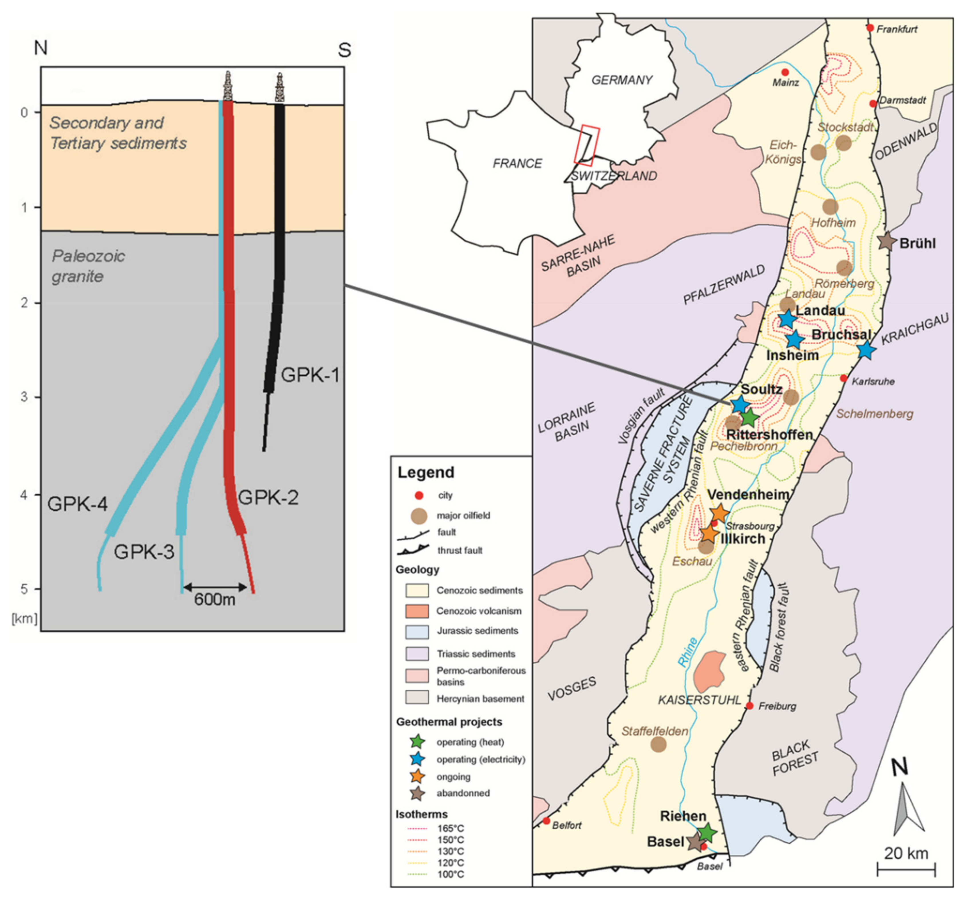
1.1. Geothermal Energy in the Upper Rhine Graben

The Upper Rhine Graben (URG) is a rifting formation, oriented NNE, part of the European Cenozoic rift system. It extends for 300 km of length, from Basel (Switzerland) in the south to Mainz (Germany) in the north. Important thermal anomalies have been identified in the URG thanks to a rich geological exploration (Figure 1, [1]). These anomalies delineate thermal gradient locally over 100 °C/km in the first km of sediments and controlled with normal faults parallel to the graben direction. The first European Geothermal research project of Soultz-sous-Forêts (SsF) was conducted initially in the early 1990s. This project was based on the Hot Dry Rock (HDR) concept, where the goal was to create an artificial heat exchanger in the basement rocks by hydraulic fracturing [2]. However, the results obtained after the drilling of the first well at SsF showed the presence of natural fluid circulation through the existing fracture network of the reservoir [3]. Since then, the Enhanced Geothermal System (EGS) technology was incorporated into future development of the URG geothermal project. This approach consists of exploiting the natural thermal brine circulation by improving, if necessary, the connection between the geothermal wells and the reservoir with various chemical, hydraulic, and thermal treatments [4].

There are several geothermal projects that have been developed in the French, German, and Swiss URG region over the past years. In France, two notable geothermal plants are in operation at SsF and Rittershoffen, respectively, for power and heat production while in Germany, three geothermal plants are in operation for power generation.

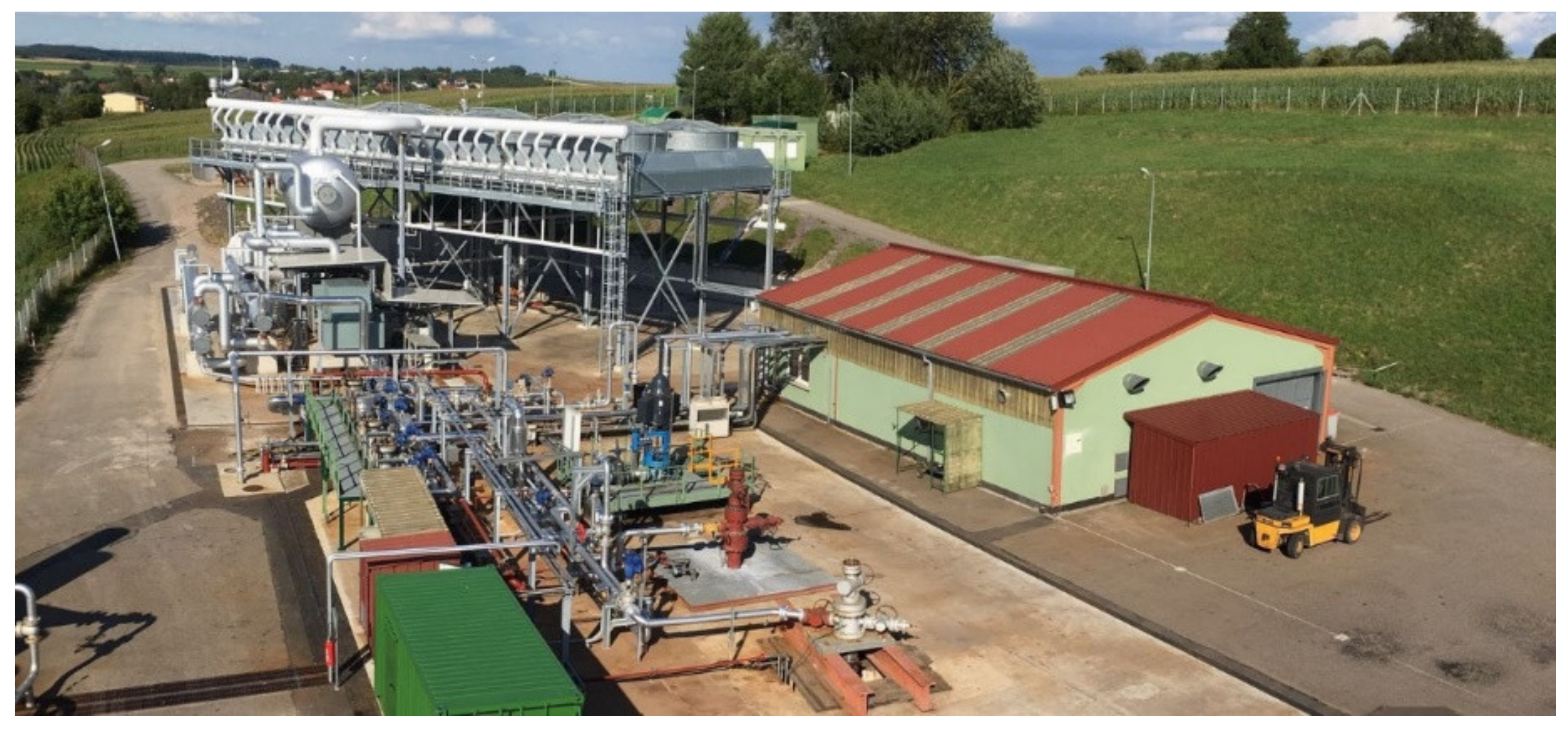
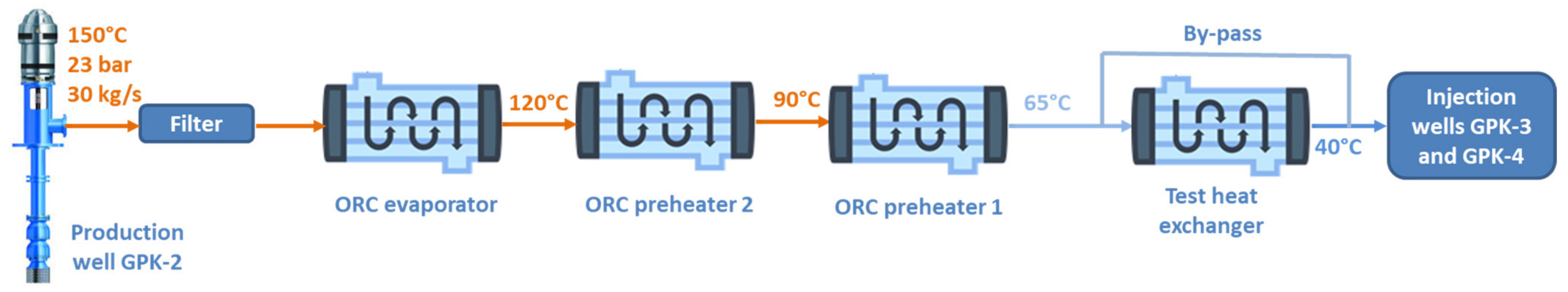
1.2. SsF Geothermal Power Plant

The Soultz-sous-Forêts geothermal project started in 1987 and is the cradle of the geothermal energy European research in granitic and fractured systems. Over 30 years of research, the geothermal site at SsF continues to exploit commercially the fractured basement for the EEIG Heat Mining. The actual geothermal system consists of three wells: one production well named GPK-2 and two injection wells named GPK-3 and GPK-4 which are drilled 5 km into the granitic basement. The geothermal brine is produced at a temperature of 150 °C, reaching the wellhead with a nominal flow rate of 30 kg/s provided by a downhole production Line Shaft Pump [5]. The installed gross capacity of the binary plant is around 1.7 MWe (Figure 2).

The geothermal brine is flowed through a system that consists of three consecutive double pass tubular heat exchangers which supply heat to an Organic Rankine Cycle (ORC) to produce electricity. The geothermal brine is then fully reinjected into the granitic basement at around 65–70 °C. The volume of reinjected brine is split between the two injection wells without the need of reinjection pumps. The well-head overpressure in the surface infrastructure is regulated by using production pump which reaches about 23 bars to keep the gas dissolved in the brine. The reinjection temperature is linked to the conversion process. The geothermal plant has been successfully producing electricity commercially since September 2016, with an availability rate of about 90% for the past four years [6]. The granite reservoir is made of a porphyritic monzogranite rich in K-feldspar megacrysts. Primary silicate minerals are quartz, plagioclase, biotite, and hornblende. A chemical analysis on the composition of the brine was taken in February 2020 (

Table 1. Composition of brine at the production well of the SsF geothermal plant [7].

GPK-2 (Production Well)
Composition of brine	Na	Ca	K	Cl	Mg	Sr	Li	SiO2	SO4	Br	Mn	NH4
(mg/L)	26,400	7020	3360	55,940	123	422	160	179	108	240	17	23.2
Composition of brine	As	Ba	Cs	Rb	B	Fe	Zn	F	I	Cu	Pb	Cd
(mg/L)	10	26	14	23	38	26.3	2.8	1.3	1.6	0.001	0.11	0.01
Composition of brine	Sb	Al	U	Ni	HCO3	COT
(mg/L)	0.06	0.05	0.001	0.0011	197	0.9

, [7]), while an analysis on the gas dissolved in the brine was taken in April 2019 (

Table 2. Composition of gas in brine at the production well of the SsF geothermal plant [7].

GPK-2 (Production Well)
Gas dissolved in brine	%vol	Partial pressure (atm)
CO2	0.882	0.882
N2	0.0908	0.0908
CH4	0.0239	0.0239

, [7]).

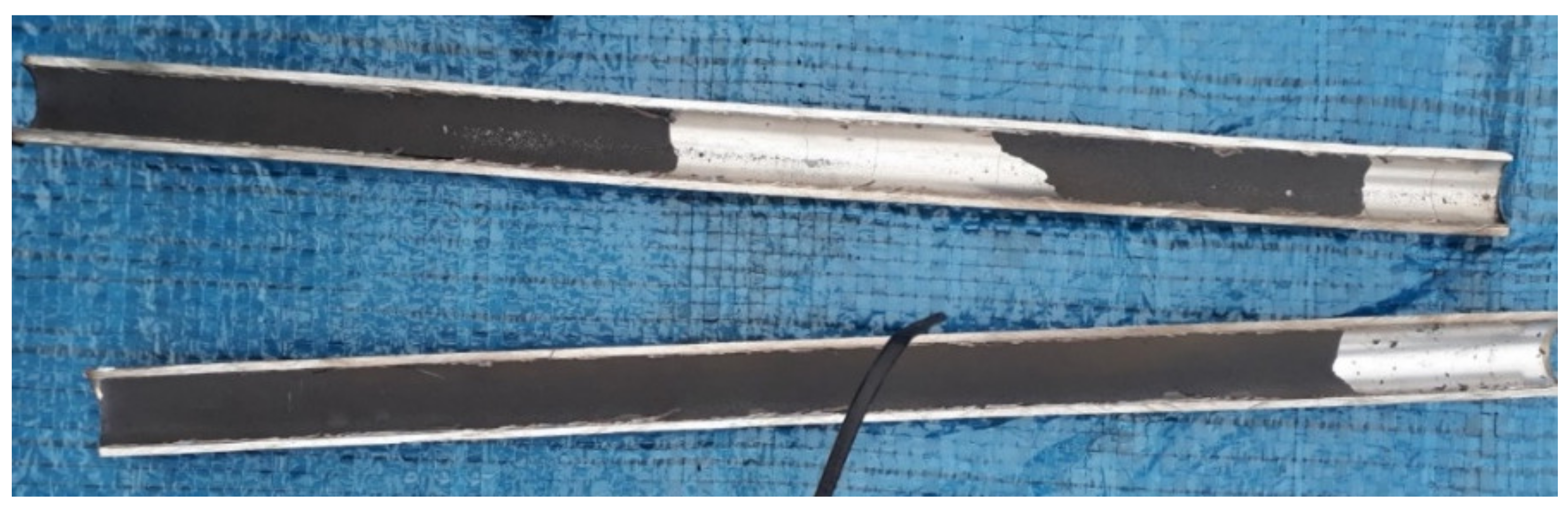
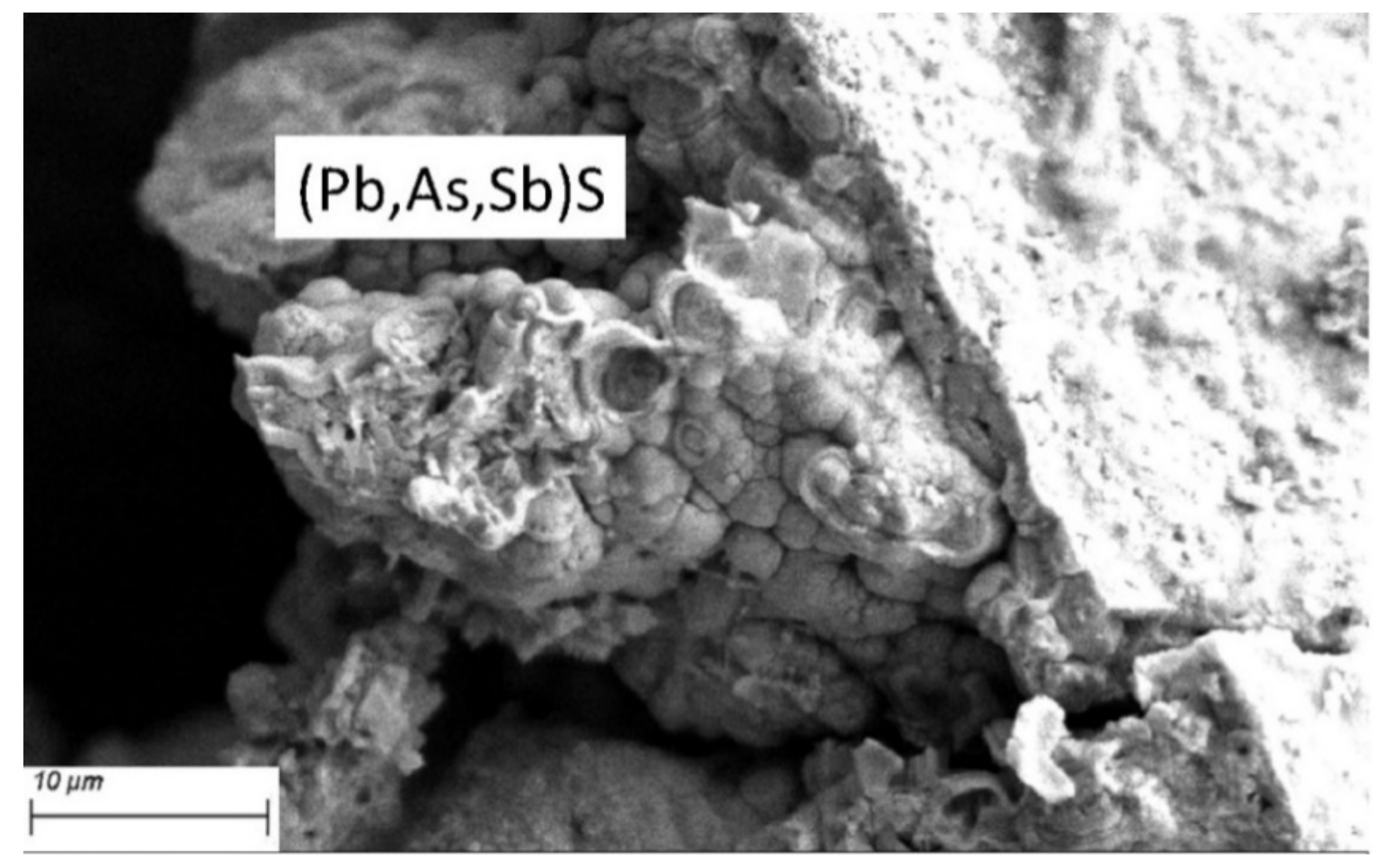
1.3. Geochemical Characterization of the Scale during Operation

In the Upper Rhine Graben region, scaling commonly occurs at the cold side of the SsF geothermal plant [8]. Therefore, in the Upper Rhine Graben, scale formation before the application of sulfate scale inhibitors was dominated by (Ba, Sr, Ca)SO₄ solid–solution scaling containing minor amounts of galena, pyrite, or poly-metallic sulfides phases [8,9,10]. The main scales observed related to deep geothermal activity have been studied not only because when represented at a significant amount of secondary precipitations they could plug the geothermal infrastructures (pipe, heat exchanger, well-head), but also because the scales have the properties to trap radiogenic elements such as ²²⁶Ra and ²¹⁰Pb in their crystalline lattices [8,9].

By using sulfate inhibitors in the Upper Rhine Graben region, barite precipitation was strongly reduced [8,11]. However, brittle grey–dark scales are still precipitating on the pipe walls consisting of PbS, and elemental Pb, As, Sb are precipitating in the geothermal infrastructures [11]. Traces of halite are present on some samples, but it corresponds to a drying residue from the geothermal brine [11]. Based on Raman spectrum of the sulfide phase, a hydrothermal Pb-Sb-Cu-sulfide (Pb₁₃CuSb₇S₂₄) has been characterized as well as an amorphous phase [11].

Several studies at SsF geothermal plant [6,12] report on the effects of the chemical treatment used to inhibit the formation of sulfate scales at SsF geothermal plant. Complementary studies have been carried out in the framework of the MEET research project at temperature below 65 °C with a test heat exchanger [13]. A typical black scale deposit at the wall of a tube pipe of this heat exchanger is shown in Figure 3. CY Cergy Paris Université conducted a study on different scales found in the test heat exchanger with a Zeiss GeminiSEM 300 Scanning Electron Microscopy, coupled with a Bruker Energy Dispersive Spectrometry. Figure 4 details this typical scale, a (Pb,As,Sb)S fibro-radiated hilly scale found at 50 °C on 1.4410 stainless steel tube [14].

Scales in the range between 150 °C and 65 °C have been sampled in June 2018 before cleaning operation in the ORC evaporator and preheaters after nearly one year of operation. Figure 5 presents a schematic drawing of the geothermal loop at SsF and the temperature gradient in the heat exchangers between the production well GPK-2 and injection wells GPK-3 and GPK4. Chemical composition of these scales has been determined using ICP MS method which is a type of mass spectrometry that uses an inductively couple plasma to ionize the sample. Scales in the range between 60 °C and 40 °C have been sampled in April 2019 in a test heat exchanger (HEX) designed with different metallurgy and installed at the SsF geothermal plant during three months in the framework of the MEET research project [13]. The latest chemical composition of scales observed at SsF geothermal plant within a range of temperature between 150 °C to 40 °C are presented in

Table 3. The mass composition of scales formed in the heat exchangers at the geothermal plant and in the test heat exchangers in percentage.

Temperature	S	Pb	Sr	Ba	Sb	As	Fe	Si	Cu	Exchanger
150	2.9%	2.0%	2.9%	0.94%	0.11%	0.53%	1.7%	3.8%	0.40%	ORC Inlet Evaporator
120	11.8%	26.5%	0.65%	1.9%	3.3%	6.6%	7.5%	8.0%	16.6%	ORC Inlet Preheater 2
90	11.2%	36.1%	0.86%	3.6%	3.1%	5.2%	8.0%	16.9%	5.1%	ORC Inlet Preheater 1
65	13.1%	46.3%	0.51%	2.2%	6.3%	7.3%	4.6%	8.4%	4.5%	ORC Outlet Preheater 1
60	13.1%	74.6%	0.01%	0.00%	6.4%	3.2%	0.07%	1.4%	0.40%	Test HEX
50	14.4%	66.5%	0.01%	0.01%	11.4%	4.3%	0.55%	1.0%	0.43%	Test HEX
40	16.7%	64.2%	0.01%	0.01%	10.9%	4.5%	0.48%	1.6%	0.36%	Test HEX

. Table 3 considers only scaling samples from tubes with 1.4410 metallurgy like the ORC heat exchanges to have a good comparison. A detail description of these scales is given by Ledésert et al. (2021) [14], and chemical composition was also determined using ICP MS method. Chemical treatment of the brine was almost the same for the two sets of scales. These scales consist of S, Pb, Sr, Ba, Sb, As, Fe, Si, and Cu elements.

The presentation of the mass percentage of scales is based on the total elements found in the scales. Certain compounds, mainly carbonates, were omitted from Table 3 because they are not the main focus of this study which is dedicated to low temperature scale formation. There are also lesser amounts of the scales deposited in the higher temperature heat exchangers (ORC heat exchangers), while more scales are deposited in the lower temperature heat exchangers (Test HEX).

Lead is found primarily at lower temperatures notably at temperatures below 120 °C. Sulfur, arsenic, silicon, and antimony are also deposited at large quantities after lead. The rest of the elements are found in smaller traces (less than 5%). The test heat exchanger has a different concentration of scales compared to the ORC heat exchangers at the geothermal plant due to the difference in temperature. In the test heat exchanger, lead has a higher concentration than those in the main exchangers. The chemical treatment on the sulfate scales proved to be effective as the quantity of barium sulfate (barite) and strontium sulfate (celestite) are found in very small quantities which are less than 4% for any point of temperature, while before the application of such treatment (Ba, Sr, Ca)SO₄ solid–solution was dominating [8].

The main objective of this study was to model the scaling phenomenon occurring in the surface pipes and heat exchangers at the SsF geothermal plant. Scaling formation was firstly modelled according to thermodynamic perspective and the results are compared to the geochemical analyses presented in Table 3 and used as references. A previous investigation was conducted on available thermodynamical databases to find the most suitable one regarding geochemical elements and possible scaling minerals. Thermodynamical modeling was then completed with kinetic modeling to better represent real operational conditions in heat exchangers. The results of both modeling are later discussed.

2. Methods

The modelling of the geochemical fluids is done through the software, PhreeqC 3.6.4 which is a computer program that is written in C++ programming language. It is designed to perform numerous aqueous geochemical calculations. PhreeqC implements several types of aqueous models depending on the database used. This program was created by the U.S. Geological Survey (USGS). PhreeqC is freely distributed by the USGS and is currently an open source software.

PhreeqC uses a pre-established thermodynamic database to perform the calculations during modelling of a fluid. Each database has different sets of elements and aqueous species as well as different thermodynamic data which are taken from different references sources. There are several databases found within the installation of the PhreeqC program. Supplementary databases were also found in the PhreeqC Users forum. There are databases taken from studies such as e THERMOCHIMIE [15] and THEREDA [16]. The PhreeqC manual [17] was referred to when performing the modelling of formation of scales with PhreeqC.

Table 4. PhreeqC databases and allocated nomenclature.

Databases	Nomenclature
Phreeqc	D1
Pitzer	D2
ColdChem	D3
Core10	D4
Frezchem	D5
Iso	D6
LLNL	D7
MINTEQ	D8
Minteq v4	D9
Pitzer_Old	D10
sit	D11
T_H	D12
WATEQ4F	D13
Thermoddem_06_2017	D14
PHREEQC_ThermoddemV1.10_15Dec2020	D15
ThermoChimie_PHREEQC_eDH_v9b0	D16
THEREDA_2020_PHRQ	D17
CEMDATA18.1-16-01-2019-phaseVol	D18
ThermoChimie_PhreeqC_SIT_oxygen_v10a	D19

shows the list of databases gathered which are listed from D1 to D19:

2.1. Verification: Elements

In order to verify the validity of the databases to be used in the modelling process, the sets of elements available within the databases were compared to the elements found in the geothermal fluid at the SsF plant. The latest chemical analysis (taken in February 2020) on the composition of the brine at the SsF plant was used to cross-reference with the sets of elements found in the databases to narrow down the list of valid databases. This analysis showed that there was high concentration of Na and Cl ions in the brine. The recent study by Bosia et al. (2021) [7] provides further details on the geochemical dataset used. Databases with more supplementary elements were taken more into consideration due to the likelihood of simulating the actual fluid. Thus, the presence of the elements in the databases are compared to the elements found in the geothermal fluid at the SsF plant (

Table 5. Geochemical elements in the databases.

	D1	D2	D3	D4	D5	D6	D7	D8	D9	D10	D11	D12	D13	D14	D15	D16	D17	D18	D19
S	x	x	x	x	x	x	x	x	x	x	x	x	x	x	x	x	x	x	x
Pb	x						x	x	x		x	x	x	x	x	x			x
Sr	x	x					x	x	x	x	x	x	x	x	x	x	x	x	x
Ba	x	x					x	x	x	x	x	x	x	x	x	x			x
Sb							x	x	x		x			x	x	x			x
As							x	x	x		x	x	x	x	x	x			x
Fe	x	x		x		x	x	x	x	x	x	x	x	x	x	x		x	x
Si	x	x		x		x	x	x	x		x	x	x	x	x	x	x	x	x
Cu	x			x			x	x	x		x	x	x	x	x	x			x
Al	x			x		x	x	x	x		x	x	x	x	x	x	x	x	x
B	x	x		x			x	x	x	x	x	x	x	x	x	x			x
Be							x	x	x					x	x
Br	x	x				x	x	x	x	x	x	x	x	x	x	x			x
Ca	x		x	x	x	x	x	x	x	x	x	x	x	x	x	x	x	x	x
Cd	x						x	x	x		x	x	x	x	x	x			x
Ce							x							x	x
Cl	x	x	x	x	x	x	x	x	x		x	x	x	x	x	x	x	x	x
Co				x			x		x		x			x	x	x			x
Cs							x				x	x	x	x	x	x	x		x
Dy							x							x	x
Er							x							x	x
Eu				x			x				x			x	x	x			x
F	x					x	x	x	x		x	x	x	x	x	x			x
Gd				x			x							x	x
Ge														x	x
Hg							x	x	x		x			x	x	x
Ho							x				x			x	x	x			x
I							x	x	x		x	x	x	x	x	x			x
In							x							x	x
K	x	x	x	x	x	x	x	x	x	x	x	x	x	x	x	x	x	x	x
La							x							x	x
Li	x	x		x			x	x	x	x	x	x	x	x	x	x			x
Lu							x							x	x
Mg	x	x	x	x	x	x	x	x	x	x	x	x	x	x	x	x	x	x	x
Mn	x	x		x			x	x	x	x	x	x	x	x	x	x			x
Mo				x			x		x		x			x	x	x			x
Na	x	x	x	x	x	x	x	x	x	x	x	x	x	x	x	x	x	x	x
Nd							x							x	x		x
Ni				x			x	x	x		x		x	x	x	x			x
P	x			x		x	x	x	x		x	x	x	x	x	x	x		x
Pd							x				x			x	x	x			x
Pr							x							x	x
Rb							x	x			x	x	x	x	x	x			x
Re							x							x	x
Rh														x	x
Sc				x			x							x	x
Sm				x			x				x			x	x	x			x
Tb							x							x	x
Tm							x							x	x
W		x					x							x	x
Y							x							x	x
Yb							x							x	x
Zn	x	x		x			x	x	x		x	x	x	x	x	x			x
HCO3	x	x		x	x	x	x	x	x	x	x	x	x	x	x	x *	x	x	x
NH4				x			x	x	x		x	x	x	x	x	x		x	x
SO3				x			x	x	x		x	x *	x *	x	x	x		x	x
SO4	x	x	x	x	x	x	x	x	x	x	x	x	x	x	x	x	x	x	x
Total	23	17	7	26	8	14	55	32	33	14	38	29	30	57	57	38	14	14	37

* = limited.

)

The geochemical elements from the Table 5 are represented in their aqueous state. From this study, the Thermoddem (D14 and D15) [18] and LLNL (D7) [19] databases, having respectively 57 and 55 elements of the 57 SsF brine chemical composition, are observed to be suitable for the purpose of this study as they possess the most amount elements found in the brine at the SsF plant. Further reference to the Thermoddem database will be the Thermoddem (D15) database instead of the Thermoddem (D14) database, because D15 is the latest version for the Thermoddem database.

2.2. Verification: Minerals

Another criterion set for the validation of the databases is the formation of probable minerals in the geothermal fluid at the SsF plant. A list of known minerals precipitated was made to compare to the minerals found in the databases. Furthermore, a list of probable minerals precipitated was made for minerals that have not been identified before in previous studies. These minerals that are susceptible to precipitation are identified by listing out minerals from the databases that consist of at least two of nine elements that are the majority in the analysis of scales conducted at the site. The nine principal elements are sulfur, lead, strontium, barium, antimony, arsenic, iron, silicon, and copper. A similar approach to the verification of elements was used in the verification of minerals in which a table with the list of minerals was cross-referenced with the database. The occurrences of known minerals and minerals susceptible to precipitation in the databases are tabulated (

Table 6. Minerals in the databases.

		Databases
Known Minerals		D1	D2	D3	D4	D5	D6	D7	D8	D9	D10	D11	D12	D13	D14	D15	D16	D17	D18	D19
Galena	PbS							x	x	x		x	x	x	x	x	x			x
Quartz	SiO2	x	x		x		x	x	x	x		x	x	x	x	x	x	x	x	x
Calcite	CaCO3	x	x		x	x	x	x	x	x	x	x	x	x	x	x	x		x	x
Anhydrite	CaSO4	x	x	x	x	x	x	x	x	x	x		x	x	x	x	x		x	x
Gypsum	CaSO4:2H20	x	x	x	x	x	x	x	x	x	x	x	x	x	x	x	x		x	x
Barite	BaSO4	x	x					x	x	x	x		x	x	x	x	x			x
Halite	NaCl	x	x	x	x	x	x	x	x	x	x	x	x	x	x	x	x	x		x
Goethite	FeOOH	x			x		x	x	x	x		x	x	x	x	x	x		x	x
Celestite	SrSO4	x	x					x	x	x	x	x	x	x	x	x	x		x	x
Arsenopyrite	FeAsS							x							x	x
Stibnite	Sb2S3							x	x	x		x			x	x	x			x
Possible Other Minerals
Hematite	Fe2O3	x			x		x	x	x	x		x	x	x	x	x	x		x	x
Strontianite	SrCO3	x						x	x	x		x	x	x	x	x	x		x	x
Svanbergite	SrAl3(PO4)(SO4)(OH)6														x	x
Sr3(AsO4)2	Sr3(AsO4)2							x				x			x	x	x			x
SrS	SrS							x				x			x	x	x			x
Anglesite	PbSO4	x						x	x	x		x	x	x	x	x	x			x
Cerussite	PbCO3	x						x	x	x		x	x	x	x	x	x			x
Alamosite	PbSiO3							x	x			x	x	x	x	x	x			x
Beudantite	PbFe3(AsO4)2(OH)5:H2O														x	x
Corkite	PbFe3(PO4)(OH)6SO4							x							x	x
Cotunnite	PbCl2							x	x	x		x	x	x	x	x	x			x
Duftite	PbCuAsO4(OH)														x	x
Hinsdalite	PbAl3(PO4)(SO4)(OH)6							x	x	x			x	x	x	x
Hydrocerussite	Pb3(CO3)2(OH)2							x		x		x	x	x	x	x	x			x
Jarosite(Pb)	Pb0.5Fe3(SO4)2(OH)6														x	x
Lanarkite	Pb2SO5							x	x	x		x	x	x	x	x	x			x
Mimetite	Pb5(AsO4)3Cl														x	x
Pb3(AsO4)2	Pb3(AsO4)2								x	x		x	x	x			x			x
Pb3SO6	Pb3SO6							x	x	x			x	x
Pb4(OH)6SO4	Pb4(OH)6SO4								x	x			x	x
Pb4SO7	Pb4SO7							x	x	x			x	x
PbSO4(NH3)2	PbSO4(NH3)2							x
PbSO4(NH3)4	PbSO4(NH3)4							x
Pb(Thiocyanate)2	Pb(SCN)2							x
Philipsbornite	PbAl3(AsO4)2(OH)5:H2O														x	x
Tsumebite	Pb2Cu(PO4)(SO4)OH							x							x	x
Realgar	AsS							x	x	x		x	x	x	x	x	x			x
Orpiment	As2S3							x	x	x		x	x	x	x	x	x			x
Bornite	Cu5FeS4				x			x							x	x
Chalcocite	Cu2S				x			x	x	x			x	x	x	x
Berthierite	FeSb2S4														x	x
	Total	12	7	3	9	4	7	33	25	25	6	21	25	25	35	35	23	2	8	23

).

The similar conclusion as before can be drawn from this verification in which the two databases, Thermoddem (D15) and LLNL (D7) are suitable for the modelling of the geothermal fluids at the SsF plant due to possessing an extensive amount of thermodynamic data on known mineral found as deposits in the plant as well as possible minerals precipitated. The LLNL database has 33 mineral datasets out of the 42 possible minerals deposited, while the Thermoddem database has 35 out of the 42 possible minerals deposited.

Another step was carried out to verify the domain of validity for the minerals in the LLNL and Thermoddem databases. The range of temperature valid for each mineral was verified to ensure that it corresponds with the maximum modelling temperature of 200 °C. For the Thermoddem database, the thermodynamic data of all the minerals are valid within 0 °C to 300 °C. On the other hand, the LLNL database has different limits for each mineral. Fortunately, the minerals that were identified in Table 6 are well within the limits proposed in the LLNL database, as the lowest maximum temperature for the minerals found is at 200 °C.

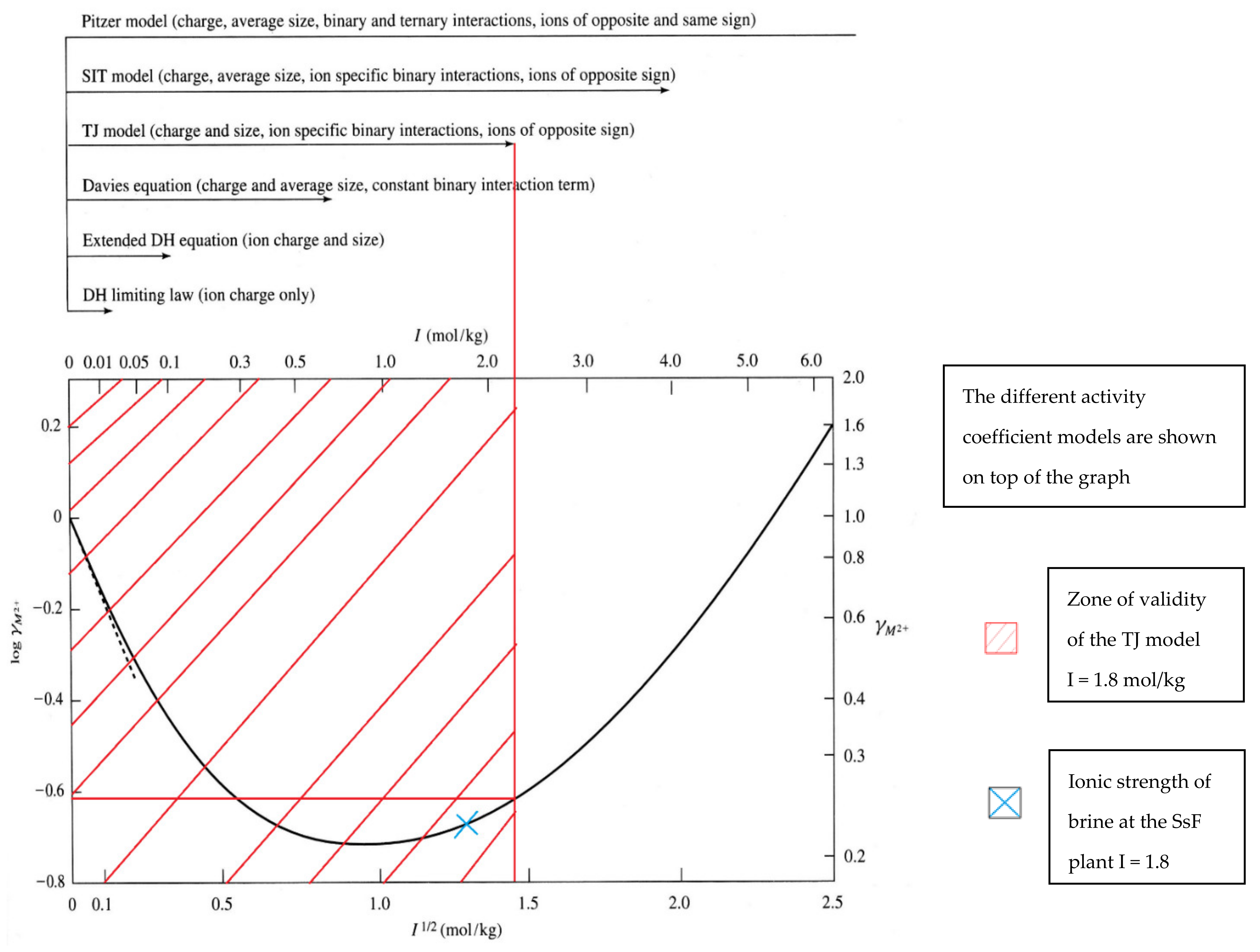
2.3. Verification: B-Dot Model Database

The two databases of interest, the Thermoddem database and the LNLL database, utilize the B-Dot equation for the calculation of activity of the elements. The B-dot model is also known as the Truesdell–Jones model (TJ model). The ionic strength of the fluid was calculated from the major elements mentioned in the most recent published geochemical datasets in Bosia et al. (2021) [7] and found to be at 1.79 mol/kg for GPK-2 and at 1.8 mol/kg for GPK-3 (

Table 7. Ionic strength calculations of the geothermal fluid sampled at GPK-2 and GPK-3.

	Molar Mass	GPK-2	GPK-3	GPK-2	GPK-3	GPK-2	GPK-3
	M (mg/mol)	mg/L		mol/L		Ionic Strength, I (mol/L or mol/kg)
Na	23,000	26,400	26,700	1.148	1.161	0.574	0.580
Cl	35,500	57,490	57,490	1.619	1.619	0.810	0.810
K	39,100	3350	3350	0.086	0.086	0.043	0.043
Ca	40,100	7020	7030	0.175	0.175	0.350	0.351
Sr	87,620	422	434	0.005	0.005	0.010	0.010
Br	79,904	240	234	0.003	0.003	0.002	0.001
Li	6940	160	163	0.023	0.023	0.012	0.012
SiO2	40,100	179	180	0.004	0.004
Total		95,261	95,581	3.063	3.077	1.799	1.807

). The unit for the ionic strength can be represented as mol/L or mol/kg since the fluid is primarily composed of water while the effects of the ions in the conversion can be ignored due to their miniscule presence in the fluid. The validity of the B-dot model is verified in Figure 6 [20] as the ionic strength is well within the limit of the TJ model for both wells. The higher the ionic strength, the less accurate the results produced. When the ionic strength of the brine exceeds the limits of the TJ model (2.2 mol/kg), the results obtained from using the B-dot databases will no longer be valid.

Since the ionic strength of the fluids at the SsF geothermal plant are well within the limits of the zone of validity, the two databases are thus used for the modelling of the fluids. Alsemgeest et al. (2021) [21] suggest being cautious when applying B-dot equation to SsF high saline geothermal brine. Nevertheless, they are also the most documented in terms of the geochemical elements and minerals.

2.4. Verification: Gas

The data available on the gases in the databases are compared to those required for modelling the geothermal fluid. The databases are then analyzed by initiating a preliminary modelling of the fluids to compare the results of the modelling with the results at the plant. For this preliminary modelling, the mixture of the gas dissolved in the brine (Table 2) was used. The conditions of the preliminary modelling are done at pH 5.2 and at two different temperatures, 80 °C and 150 °C. The saturation pressure of each database is compared and analyzed. For this analysis, the Thermoddem database, the LLNL database, and the Pitzer database were used. For the Thermoddem database and the LLNL database, as they were deemed suitable for the modelling of scales through the verification of elements and minerals, they are thus analyzed for the verification of gases. Even though the Pitzer database lacks several data on the elements and minerals, it is still considered for modelling of dissolved gases in the geothermal fluid because this database uses a different model for the calculation of activity of the elements. This may then give a more accurate result in the modelling of dissolved gases in the geothermal fluid. The results of the preliminary modelling at two different temperatures steps in terms of saturation pressure with the three databases are recorded in

Table 8. Results of the saturation pressure of SsF gas for each database at two temperature steps.

Temperature (°C)	Pitzer	LLNL	Thermoddem
80	14 atm	10 atm	10 atm
150	18 atm	15 atm	16 atm

.

The LLNL and Thermoddem databases give out a similar result at both tested temperature while the Pitzer database shows a higher pressure compared to the two previous databases (Table 8). The saturation pressure obtained from modelling at 150 °C with the Pitzer database (18 atm = 18.2 bar) is closer to the actual case observed at the SsF plant [22] at the same temperature which ranges between 18.0 and 18.5 bar at relative pressure. The Thermoddem and LLNL databases provided results outside the range of saturation pressure observed at the SsF plant. Thus, the Pitzer database is found to be more suitable than the Thermoddem and LLNL databases for the gas modelling of the SsF plant.

Overall, the Thermoddem database was selected for the modelling of the formation of scales in the geothermal fluids as this database has more data than the LLNL database on the geochemical elements and possible minerals precipitated. Furthermore, the Thermoddem database has been compiled by a French geological survey company, BRGM which is specifically designed for waste derived from natural fluid precipitation [18]. As for modelling of the dissolved gas in the fluid, the Pitzer database was observed to have given a more satisfactory result as mentioned in the previous paragraph. Thus, the Pitzer database should be used for the modelling of the solubility of gas in the geothermal fluid.

2.5. Scale Modelling

When modelling the formation of scales with PhreeqC, the physical properties of the fluids such as the temperature, pressure and pH of the fluid are inputted into the software. The initial temperature, pressure and pH of the fluid are 25 °C, 1 bar, and pH 5.2 respectively representative of the laboratory conditions for brine analysis. The temperature and pressure were later changed to the production conditions of the brine at the SsF geothermal plant which are at 150 °C and 20 bars respectively. The pH of the fluid is also adjusted by the software to reflect the temperature and the composition of the fluid, thus there was no need to modify it. The unit for the concentration of each component in the fluids is also user-defined. In the case of this study, the unit used is in mg/kgw where kgw stands for a kilogram of water. Thus, the unit mg/kgw is the mass in milligrams of the element for each kilogram of water.

The formation of scales at the SsF plant is initially modeled by using thermodynamic modelling. This method uses the thermodynamic database researched in the previous section. The saturation index of each mineral is studied in this modelling process. For any minerals with a saturation index equal or higher than zero for the conditions of the fluid at the geothermal plant, that mineral can potentially precipitate. The amount of minerals precipitated was then calculated. This method provided insight on the potential minerals that could precipitate aside from the minerals already observed in previous studies such as those mentioned in Scheiber et al. (2012) [8], Sanjuan et al. (2011) [9], and Nitschke (2012) [10]. However, this method is limited to cases where thermodynamic equilibrium is reached.

Kinetic modelling was also considered to represent accurately the situation of the formation of scales at the geothermal plant. For this method, the amount of time that the fluids pass through the plant’s exchangers is needed. It takes around 3 min for the fluid to circulate from the entrance of the first ORC heat exchanger to the exit of the final ORC heat exchanger. In these conditions, the kinetics of the reaction is also a crucial factor for the kinetic modelling. The kinetic data for chalcopyrite, galena, orpiment, and pyrite was taken from the database made by Zhang et al. (2019) [23]. The kinetic constant for stibnite was taken from Biver et al. (2011) [24] and adjusted into a modified kinetic equation for galena. For other minerals without any kinetic data, a modified kinetic equation of a similar mineral was used. The amount of minerals precipitated is calculated using its kinetic equation. This method refers to the saturation index of the mineral before calculating with the kinetic information available. As stated before, when the saturation index of the mineral is below zero, the kinetic calculation is skipped as the mineral does not precipitate. The duration for the kinetic modelling at each temperature was set to one minute because the velocity of the brine is estimated to be slightly less than 1 m/s and the length of the tubes of heat exchanger (30 m). This gives a duration of about 30 s to pass through a heat exchanger. Another 30 s was added to take into account the head cover and the pipes between each heat exchanger.

3. Results

As mentioned in the previous section, the modelling of scales in the geothermal fluids was done in Phreeqc with the Thermoddem database. For this modelling sequence, the range of temperature and pressure were set. The temperature starts from 150 °C which is the highest observable temperature at the SsF plant. The temperature then reduces until the lowest temperature found in the test heat exchanger which is at 40 °C. Additionally, two fictional temperatures were added which are at 175 °C and 200 °C in order to simulate the influence of such high temperatures on the formation of scales. These two temperatures are representative of temperatures found in the geothermal reservoir that is four to five kilometers deep under. The pressure was then fixed at 20 bars to simulate the exact conditions at the SsF geothermal plant.

3.1. Thermodynamic Modelling

The precipitation of the minerals was first studied through the observation made on the saturation index of each mineral. For the minerals with a saturation index equal or higher than zero, they are minerals that could possibly be present in the scales at thermodynamic equilibrium (Appendix A,

Table A1. Saturation Index of minerals with potential to precipitate.

Pressure (bar)		20
Temperature (°C)		40	50	60	65	90	120	150	175	200
SiO2	Amorphous_silica	0.45	0.38	0.32	0.29	0.16	0.03	−0.08	−0.16	−0.24
CaSO4	Anhydrite	−0.98	−0.88	−0.78	−0.73	−0.53	−0.32	−0.1	0.08	0.25
Cu1.75S	Anilite	2.61	1.97	1.31	0.97	−0.55	−1.95	−3.05	−3.86	−4.65
FeAsS	Arsenopyrite	−0.52	−0.28	−0.04	0.06	0.3	0.13	−0.24	−0.58	−0.9
BaSO4	Barite	1.24	1.11	0.99	0.93	0.67	0.4	0.21	0.1	0.01
FeSb2S4	Berthierite	1.33	1.25	1.17	1.13	0.92	0.63	−0.02	−1.48	−3.15
Cu5FeS4	Bornite (alpha)	17.03	15.3	13.5	12.59	8.22	3.83	0.17	−2.56	−5.19
SiO2	Chalcedony	1.16	1.05	0.96	0.91	0.72	0.52	0.34	0.21	0.1
Cu2S	Chalcocite (alpha)	2.75	2.01	1.24	0.85	−0.89	−2.45	−3.66	−4.53	−5.38
CuFeS2	Chalcopyrite (alpha)	6.21	6.07	5.91	5.8	5.12	4.08	3.01	2.17	1.36
SiO2	Coesite (alpha)	0.64	0.55	0.47	0.43	0.26	0.09	−0.05	−0.16	−0.26
CuS	Covellite	1.42	1.07	0.71	0.53	−0.36	−1.28	−2.09	−2.7	−3.28
SiO2	Cristobalite (alpha)	0.89	0.8	0.72	0.68	0.52	0.35	0.21	0.1	0
SiO2	Cristobalite (beta)	0.83	0.74	0.66	0.62	0.47	0.31	0.17	0.07	−0.02
Cu1.934S	Djurleite	2.76	2.05	1.3	0.93	−0.76	−2.29	−3.47	−4.34	−5.18
Fe10S11	Fe10S11	−19.75	−15.47	−11.34	−9.49	−2.77	0.56	1.65	1.98	2.14
Fe11S12	Fe11S12	−21.56	−16.83	−12.28	−10.23	−2.81	0.92	2.19	2.61	2.84
Fe7.016S8	Fe7.016S8	−11.61	−8.67	−5.83	−4.55	0.01	2.12	2.67	2.74	2.72
Fe9S10	Fe9S10	−16.97	−13.14	−9.45	−7.79	−1.8	1.11	2	2.23	2.31
PbS	Galena	2.57	2.54	2.51	2.49	2.18	1.6	1	0.53	0.05
FeS2	Marcassite	4.15	4.39	4.63	4.72	4.87	4.42	3.73	3.13	2.56
As2S3	Orpiment	0.92	0.97	1.04	1.04	0.58	−0.82	−2.6	−4.1	−5.52
FeS2	Pyrite	4.84	5.06	5.28	5.36	5.45	4.96	4.23	3.6	3
SiO2	Quartz (alpha)	1.43	1.31	1.21	1.16	0.95	0.73	0.54	0.4	0.28
SiO2	Quartz (beta)	1.21	1.11	1.02	0.97	0.78	0.59	0.42	0.29	0.18
Na2(Fe3Fe2)Si8O22(OH)2	Riebeckite	−7.54	−6.95	−6.34	−6.05	−4.66	−3.17	−1.68	−0.44	0.8
Sb2S3	Stibnite	3.25	2.76	2.29	2.08	1.25	0.7	0.02	−1.4	−3.01

). A list of potential minerals present within the set range of temperature was constructed from the observation of the saturation index of each mineral (

Table 9. Presence of potential minerals at the set range of temperature according to saturation index.

Pressure (bar)		20
Temperature (°C)		40	50	60	65	90	120	150	175	200
Known Minerals
SiO2	Amorphous_silica	x	x	x	x	x	x
CaSO4	Anhydrite								x	x
Sb2S3	Stibnite	x	x	x	x	x	x	x
FeAsS	Arsenopyrite				x	x	x
BaSO4	Barite	x	x	x	x	x	x	x	x	x
CuFeS2	Chalcopyrite (alpha)	x	x	x	x	x	x	x	x	x
PbS	Galena	x	x	x	x	x	x	x	x	x
SiO2	Quartz (alpha)	x	x	x	x	x	x	x	x	x
SiO2	Quartz (beta)	x	x	x	x	x	x	x	x	x
Possible Other Minerals
Cu1.75S	Anilite	x	x	x	x
FeSb2S4	Berthierite	x	x	x	x	x	x
Cu5FeS4	Bornite (alpha)	x	x	x	x	x	x	x
SiO2	Chalcedony	x	x	x	x	x	x	x	x	x
Cu2S	Chalcocite (alpha)	x	x	x	x
SiO2	Coesite (alpha)	x	x	x	x	x	x
CuS	Covellite	x	x	x	x
SiO2	Cristobalite (alpha)	x	x	x	x	x	x	x	x	x
SiO2	Cristobalite (beta)	x	x	x	x	x	x	x	x
Cu1.934S	Djurleite	x	x	x	x
Fe10S11	Fe10S11						x	x	x	x
Fe11S12	Fe11S12						x	x	x	x
Fe7.016S8	Fe7.016S8					x	x	x	x	x
Fe9S10	Fe9S10						x	x	x	x
FeS2	Marcassite	x	x	x	x	x	x	x	x	x
As2S3	Orpiment	x	x	x	x	x
FeS2	Pyrite	x	x	x	x	x	x	x	x	x
Na2(Fe3Fe2)Si8O22(OH)2	Riebeckite									x

).

The next step for the modelling of scales formation at the SsF geothermal plant is to calculate the quantity of minerals precipitating in the given temperature range. An initial modelling based on the present minerals (Table 9) was done and the results showed that not all minerals with a positive saturation index precipitated (

Table 10. Mineral precipitated for thermodynamic modelling (For 40–200 °C).

Known Minerals
Minerals precipitated according to saturation index		Minerals considered for thermodynamic modelling
SiO2	Amorphous silica	CuFeS2	Chalcopyrite (alpha)
CaSO4	Anhydrite	PbS	Galena
BaSO4	Barite	Sb2S3	Stibnite
CuFeS2	Chalcopyrite (alpha)
PbS	Galena
SiO2	Quartz (alpha)
SiO2	Quartz (beta)
Sb2S3	Stibnite
Possible Other Minerals
Minerals precipitated according to saturation index		Minerals considered for thermodynamic modelling
Cu1.75S	Anilite	Cu1.75S	Anilite
FeSb2S4	Berthierite	FeSb2S4	Berthierite
Cu5FeS4	Bornite (alpha)	Cu5FeS4	Bornite (alpha)
SiO2	Coesite (alpha)	CuS	Covellite
CuS	Covellite	FeS2	Marcasite
SiO2	Cristobalite (beta)	As2S3	Orpiment
FeS2	Marcasite	FeS2	Pyrite
As2S3	Orpiment
FeS2	Pyrite

, left side). This is explained by the higher saturation index of several minerals which have higher priority to precipitate. The results of the thermodynamic modelling (

Table 11. Results of first thermodynamic modelling in weight percentage.

		Temperature (°C)
	M (g/mol)	40	50	60	65	90	120	150	175	200
As	74.922	0.00%	0.00%	0.00%	0.00%	0.00%	0.00%	0.00%	0.00%	0.00%
Ba	137.33	2.3%	2.1%	4.4%	4.8%	5.1%	5.5%	4.9%	0.00%	0.00%
Ca	40.08	0.00%	0.00%	0.00%	0.00%	0.00%	0.00%	0.00%	5.0%	9.7%
Cu	63.546	0.00%	0.00%	0.00%	0.00%	0.00%	0.00%	0.00%	0.00%	0.00%
Fe	55.847	0.60%	0.52%	0.45%	0.65%	1.3%	1.4%	1.4%	1.2%	1.1%
O	15.999	51.6%	51.7%	50.8%	50.4%	49.5%	49.3%	49.5%	50.8%	49.9%
Pb	207.2	0.01%	0.01%	0.02%	0.00%	0.02%	0.00%	0.01%	0.00%	0.01%
S	32.066	1.2%	1.1%	1.5%	1.9%	2.7%	2.9%	2.7%	5.4%	9.0%
Sb	121.75	0.01%	0.01%	0.02%	0.01%	0.02%	0.02%	0.01%	0.00%	0.00%
Si	28.086	44.3%	44.5%	42.8%	42.3%	41.3%	41.0%	41.4%	37.6%	30.3%

) from using the minerals of the left side of Table 10 showed that majority of the minerals consist of silicates because of the high concentration of O and Si. At the range of temperature between 40 °C to 150 °C, silicate scales are not usually found at high amounts at the SsF geothermal plant.

To have a better focus on the modelling of scales at the SsF geothermal plant, the minerals considered for the thermodynamic model were then identified (Table 10, right side). Barite and celestite were excluded from future modelling sequence, because inhibitors are used by the operator to prevent the formation of these scales. For silicates, it is suspected that kinetic reaction prevents their deposition. That is why they were excluded to focus on the primary elements found in the scales found at the SsF geothermal plant as mentioned before. The results of the calculation are done at the different temperatures (

Table 12. Results of refined thermodynamic modelling in weight percentage.

		Temperature (°C)
	M (g/mol)	40	50	60	65	90	120	150	175	200
As	74.922	0.00%	0.00%	0.00%	0.00%	0.00%	0.00%	0.00%	0.00%	0.00%
Cu	63.546	0.04%	0.00%	0.00%	0.00%	0.00%	0.00%	0.00%	0.00%	0.00%
Fe	55.847	45.6%	45.6%	44.8%	45.9%	45.8%	46.2%	46.2%	46.5%	46.4%
Pb	207.2	0.72%	0.50%	1.5%	0.25%	0.52%	0.07%	0.43%	0.04%	0.30%
S	32.066	52.8%	52.9%	52.3%	53.1%	53.0%	53.2%	53.2%	53.4%	53.3%
Sb	121.75	0.77%	1.0%	1.5%	0.76%	0.67%	0.48%	0.17%	0.00%	0.00%

).

For each step of temperature, the modelling results show that sulfur and iron are the major elements with concentrations of 45% and 53% respectively (Table 12). On the other hand, the total amount of the other elements represents less than 3% of the total. Copper is only found at 40 °C and in extremely small quantities. Antimony and lead are also found in small quantities (less than 1.5%) at any given step of temperature.

3.2. Kinetic Modelling

The results given out by the calculation of the thermodynamic model gives insight on the precipitation of the minerals at thermodynamic equilibrium which may not necessarily be respected in the conditions studied. Modelling done from a kinetics aspect was proposed and the results from the thermodynamic model were compared and complimented with literature review and field knowledge to select the proper minerals which could precipitate. The kinetic information was mainly obtained from Zhang et al. (2019) [23] as mentioned in the Section 2. Initially, the model had little modification to the kinetic information used from the source with exception for minerals lacking their kinetic information. Rates equations for metal sulfides including the concentration of oxygen into the calculation are removed, because they serve no purpose due to the little to no oxygen content in the brine at the SsF geothermal plant.

For the initial model, two different sets of minerals were considered. The first set of minerals are galena (PbS), orpiment (As₂S₃), pyrite (FeS₂), amorphous silica (SiO₂), quartz (alpha) (SiO₂), and stibnite (Sb₂S₃). Galena and stibnite are known minerals already observed at the SsF plant [14]. Pyrite was considered over arsenopyrite (AsFeS) and chalcopyrite (CuFeS), because pyrite has a higher saturation index than arsenopyrite (Appendix A, Table A1); thus pyrite is more susceptible to precipitate than arsenopyrite. Chalcopyrite was dismissed as the principal provider of Fe precipitation because there is only a small amount of copper found in the analysis done at the SsF plant (Table 3) which is negligible compared to the quantity of Fe found. As for orpiment, this mineral is the only representative for presence of the element As. For amorphous silica and quartz (alpha), they were considered as they had a major influence in the thermodynamic modelling. Unfortunately, the desired modelling conditions do not fall within the domain of validity for the initial kinetic model created. For the formation of galena, this model is only valid for a temperature between 25 °C to 70 °C and a pH between one and three. For the formation of pyrite, this model is only valid for a temperature between 20 °C to 40 °C and a pH between one and four. For both cases, the range of pH is too acidic compared to the actual case. The model for the formation of orpiment is only valid for a temperature between 25 °C to 40 °C and a pH between 7.3 and 9.4 which is too alkaline. For the formation of amorphous silica, the model is only valid for a pH around 5.7, which is a bit too alkaline compared to the pH of the fluid at the SsF geothermal plant. For the formation of quartz (alpha), the model is within the proper zone of validity. Regardless, this model was used as an initial approach to modelling the minerals precipitated. For stibnite, no source for its kinetic information aside from its kinetic constant is found [24]. Thus, the kinetic equation of galena was taken and modified to suit the kinetic rate of stibnite. Minerals such as barite and celestite were not added, because their exclusion serves as a proxy to their inhibition by chemical treatment.

The second set of minerals consists of the same minerals from the first set, but excluding amorphous silica and quartz (alpha). These two minerals were excluded to better focus on the main minerals identified in the scales at the SsF geothermal plant. The modelling with both set of minerals was only done from 200 °C to 65 °C as it is complicated to model the circulation of fluids in the pipes between the ORC heat exchangers and the test heat exchangers. Furthermore, the residence time and the surface area of the heat exchangers in contact with the brine are different in both cases which will thus further complexify the model. To simplify the model, the ORC heat exchangers were chosen as the standard for the temperature to be modelled.

The first results showed that for the temperatures between 65 °C and 150 °C, S and Fe are the major elements in the simulated scales (

Table 13. Results for initial kinetics model with first set of minerals in weight percentage.

Temperature	Pb	Fe	As	Sb	S	Si	O	Majority
65	8.88%	40.77%	0.14%	1.13%	48.73%	0.16%	0.18%	S
90	2.14%	45.11%	0.01%	0.04%	52.16%	0.24%	0.28%	S
120	0.95%	44.67%	0.00%	0.01%	51.45%	1.4%	1.6%	S
150	0.60%	35.72%	0.00%	0.00%	41.12%	10.5%	12.0%	S
175	0.22%	15.66%	0.00%	0.00%	18.01%	30.9%	35.2%	O
200	0.01%	3.80%	0.00%	0.00%	4.36%	42.9%	48.9%	O

). From 175 °C onwards, Si and O are the major elements while Pb, As, and Sb are found in negligible amounts.

The results show that sulfur is the majority for every step of temperature taking up to 53.4% of the composition of scales (

Table 14. Results for initial kinetics model with second set of minerals in weight percentage.

Temperature	Pb	Fe	As	Sb	S	Majority
65	8.9%	40.9%	0.14%	1.1%	48.9%	S
90	2.2%	45.4%	0.01%	0.04%	52.4%	S
120	0.98%	46.0%	0.00%	0.01%	53.0%	S
150	0.78%	46.1%	0.00%	0.00%	53.1%	S
175	0.64%	46.2%	0.00%	0.00%	53.2%	S
200	0.11%	46.5%	0.00%	0.00%	53.4%	S

). Iron is shown to be in second largest mass quantity with a weight percentage of around 46% except at 65 °C which is at 40.9%. Lead is shown to be in smaller quantity such as 8.9% at 65 °C and 2.2% at 90 °C, respectively. Between 200 °C and 120 °C, the quantity of lead is less than 1%. As for antimony and arsenic, both are found in extremely small quantities where antimony is at 1.1% and arsenic is at 0.14% for the temperature of 65 °C. Antimony and arsenic are not found at higher temperatures (above 150 °C).

4. Discussion

4.1. Introduction

In this discussion, an analysis is done on the thermodynamic modelling and the kinetic modelling to identify the utility and shortcomings of each method. The factors that affect the results of each method are also discussed. Modifications were done on the kinetic model to better fit with the chemistry of scale observed at the SsF plant. Finally, new perspectives are proposed and discussed to improve further the proposed predictive kinetic model.

4.2. Thermodynamic Modelling Analysis

The thermodynamic modelling provides insight on possible precipitation of minerals at each temperature step. It can be observed that minerals containing strontium such as celestite were not listed as minerals precipitated by the modelling software (Table 9). In the analysis made on the scales at the SsF plant, traces of strontium were found and were identified to be celestite [8,9]. This discrepancy can be explained by the fact that the supposed mineral found at the plant, celestite, dissolves in favor of the precipitation of barite [25]. Since the results are calculated at thermodynamic equilibrium, the total consumption of celestite was already considered during the calculations made by PhreeqC. Another explanation is that the PhreeqC software does not consider the existence of solid solutions like barium/strontium sulfates. Hence, the software considers barite over celestite for their precipitation. Thus, strontium was excluded from the comparison of the weight percentage of the elements between the Ssf plant analyses, the thermodynamic models, and the kinetic models. Barite is shown to potentially precipitate at the given range of temperature (Table 9). However, as the temperature decreases, the saturation index of barite increases thus increasing its potential to precipitate (Appendix A, Table A1). A similar situation is observed in the formation of galena, albeit with a higher saturation index. For pyrite, it can also potentially precipitate at the given range of temperature. Its saturation index increases from 200 °C to 90 °C in which it starts to decrease thereafter. Precipitation of native metals could not be observed in neither thermodynamics modelling nor kinetics modelling, because the modelling software cannot take into account their formation.

When silicates were considered for the thermodynamic model, the results (Table 11) showed that Si and O take up the majority of the elements until it rendered the rest of the elements negligible in the simulated scales. This is not the case at the SsF geothermal plant as there were tiny amounts of silicate in the actual analyses. A second model was constructed by excluding the silicates to have a better focus on the known minerals found at the geothermal plant.

The amount of galena formed in the thermodynamic models is greatly inferior to the actual scaling at the SsF geothermal plant (

Table 15. Comparison between Soultz-sous-Forêts, thermodynamic model, and kinetic model results in relative percentage by weight.

	Temperature	65	90	120	150
Pb	SsF plant analyses	59.7%	56.8%	39.9%	27.3%
	Thermodynamic model 1	0.00%	0.02%	0.00%	0.01%
	Thermodynamic model 2	0.25%	0.52%	0.07%	0.43%
	Kinetic Model 1	8.9%	2.1%	0.95%	0.60%
	Kinetic Model 2	8.9%	2.2%	0.98%	0.78%
Fe	SsF plant analyses	5.9%	12.6%	12.1%	23.3%
	Thermodynamic model 1	0.65%	1.34%	1.37%	1.36%
	Thermodynamic model 2	45.9%	45.8%	46.2%	46.2%
	Kinetic Model 1	40.8%	45.1%	44.7%	35.7%
	Kinetic Model 2	40.9%	45.4%	46.0%	46.1%
As	SsF plant analyses	9%	8%	13%	7%
	Thermodynamic model 1	0%	0%	0%	0%
	Thermodynamic model 2	0.00%	0.00%	0.00%	0.00%
	Kinetic Model 1	0.14%	0.01%	0.00%	0.00%
	Kinetic Model 2	0.14%	0.01%	0.00%	0.00%
Sb	SsF plant analyses	8%	5%	3%	2%
	Thermodynamic model 1	0.01%	0.02%	0.02%	0.01%
	Thermodynamic model 2	0.76%	0.67%	0.48%	0.17%
	Kinetic Model 1	1.13%	0.04%	0.01%	0.00%
	Kinetic Model 2	1.1%	0.04%	0.01%	0.00%
S	SsF plant analyses	17%	18%	32%	41%
	Thermodynamic model 1	1.9%	2.7%	2.9%	2.7%
	Thermodynamic model 2	53.1%	53.0%	53.2%	53.2%
	Kinetic Model 1	48.73%	52.2%	51.5%	41.1%
	Kinetic Model 2	48.9%	52.4%	53.0%	53.1%

). There is an unusually high amount of iron and sulfur in the thermodynamic modelling. Furthermore, the quantity of lead is still in the minority. Another problem is that the thermodynamic modelling simulates the precipitation of the minerals over a great amount of time which is until the fluid reaches thermodynamic equilibrium. At the SsF geothermal plant, the precipitation of the minerals is not necessarily at thermodynamic equilibrium since the residence time of the brine in the exchanger is only around three minutes. Furthermore, the initial amount of lead (Pb) (Table 2) is smaller than the rest of elements in the brine. This could explain the low amount of lead found in simulated scales compared to the other elements in this modelling method. Thus, the thermodynamic model proved to be not sufficient for the prediction of formation of scales at the SsF geothermal plant and kinetic effect must be considered.

4.3. Kinetic Modelling Analysis

The kinetics model with the first set of minerals (Table 13) showed improvements in the results when compared to the first thermodynamic model (Table 11). The kinetic model with the first set of minerals (Table 13) has significantly reduced the Si and O contents for the temperatures between 65 °C and 150 °C. This confirms that the kinetic effect controls the absence of silicates in the SsF scales.

However, for this range of temperature, sulfur (S) and iron (Fe) have the highest concentration with the highest percentage being 52.2% and 45.1% respectively (Table 15). Regardless, the concentration of each element for the kinetic model 1 does not reflect the actual concentration found in the SsF plant analyses.

As for the kinetic model 2, it showed similar improvements in the results to the results of kinetic model 1. At 65 °C, the quantity of lead has increased from 0.25% (thermodynamic model 2) to 8.9% (kinetic model 2) in the composition of elements found in the modelled scales (Table 14). However, iron and sulfur are still the major elements in the modelled scales. The lack of kinetic information on the formation of stibnite could also lead to inaccuracies in the results such as the low amount of antimony. In addition, the amount of sulfur present at each temperature is larger than the actual case. The discrepancies can be explained by the conditions of the modelled scales being outside the domain of validity for temperature and pH of the kinetic information used.

Therefore, to better simulate the scale formation at the SsF geothermal plant, a modified version of the initial model was created. In this second model, the kinetic information of the minerals was modified to reflect closely to the analyses done at the geothermal plant. The kinetic information was purposely modified until the model produces a result similar to the ones obtained at SsF geothermal plant at one temperature step. The modification was done iteratively until the results were in an approximate range of the actual case. Thus, the modified kinetic information is not indicative of any actual kinetic values. The two minerals (arsenopyrite and chalcopyrite) were added to compensate for the low amount of arsenic and the high amount of sulfur and iron. The kinetic information of chalcopyrite is taken from Zhang et al. (2019), whereas no kinetic data was found on arsenopyrite. Thus, the kinetic data of chalcopyrite was taken and modified for arsenopyrite. Next, the kinetic rate of pyrite was slowed down as this mineral has the greatest influence on the increases of percentage of iron and sulfur (

Table 16. Modification of the first kinetic model. n_x: representing the index used in the rates equation (Appendix B).

	Initial Model	Modified Model
Arsenopyrite	n = 1.68	n = 0.8
Orpiment	n2 = −1.26	n2 = −1.48
Stibnite	n = 0.5	n = 0.475
Pyrite	n1 = −0.5	n1 = −0.25
	n3 = 0.5	n3 = 0.55

). Overall, the kinetic information of all the minerals except galena and chalcopyrite was modified to obtain a general model for the formation of scales.

The modified model presented a result that is closer to the analyses of scales at the geothermal plant (Table 15 and

Table 17. Mass of elements in percentage for modified kinetics model.

Temperature	Pb	Fe	As	Sb	S	Cu	Majority
65	52.2%	5.0%	9.0%	8.5%	22.5%	2.8%	Lead
90	45.6%	16.0%	9.2%	1.2%	25.2%	2.8%	Lead
120	34.9%	23.5%	7.0%	0.42%	29.6%	4.6%	Lead
150	40.1%	22.7%	0.00%	0.01%	32.3%	4.9%	Lead
175	41.7%	23.0%	0.00%	0.00%	32.8%	2.5%	Lead
200	14.4%	38.0%	0.00%	0.00%	45.8%	1.8%	Sulfur

). The percentage of sulfur is still higher than the actual case, but the increase in quantity of sulfur scales better than the unmodified kinetic information models. The quantity of iron is higher than the actual case for the temperature between 90 °C and 150 °C. In addition, there are no other minerals that contain antimony and arsenic that has a positive saturation index for temperatures above 120 °C. This leads to having small and negligible quantities of both elements at the mentioned temperature. All things considered, this model allows a rough prediction on the scale formation when operating the plant with sulfate scales inhibitors at the SsF geothermal plant as there is only a small deviation between simulated results and the actual case. The model becomes less accurate at higher temperatures such as at 150 °C, because of the lack of antimony and arsenic at this temperature (Table 15).

4.4. New Perspectives

For the modelling of scales for the SsF geothermal plant, a lot of information was lacking such as the kinetic information that is suited for the operating conditions of the plant. Future studies and analyses on the precipitation of the minerals are to be arranged to obtain the missing kinetic information and challenge the modified kinetic model. A laboratory study is necessary to investigate the precipitation of minerals at conditions of the SsF geothermal plant which is at around pH 5.2 and the temperature range of the ORC heat exchangers. The kinetic model for pyrite might also not be suitable for modelling the scales at the pH, pressure, and temperature of SsF geothermal plant which led to inaccuracies in the results pertaining to the amount of Fe and S. Therefore, the kinetic information of the precipitation of pyrite as well as galena, arsenopyrite, chalcopyrite, arsenides, sulfosalts, selenides, and other base metal sulfides are needed to be determined through this laboratory study so that a proper kinetic model can be constructed.

Furthermore, the inhibition of sulfates such as barium and celestite was just excluded from the calculation due to lack of information on their kinetics. Therefore, the inhibition process should also be analyzed and studied to obtain its kinetic information that can be integrated into the kinetic model. With a proper kinetic model, a more precise result can be obtained through the simulation on the formation of scales in the pipes and exchanger at the geothermal plant. Besides that, other reactions aside from precipitation should also be studied and integrated into the model such as the possibility of heavy metal corrosion in the pipes and heat exchanger, as mentioned in Lichti and Brown (2013) [26] and Lichti et al. (2016) [27]. This phenomenon should be studied at the SsF geothermal plant and be verified whether it affects the amount of scales formed at the plant. A study should also be conducted on the possibility of a chemical interaction between FeS and PbS. The results from the laboratory studies on this chemical interaction at the SsF operational condition could be integrated into the current prediction model for a more accurate result.

5. Conclusions

From the geochemical analyses done on the SsF geothermal plant, lead is found to be the major element in the composition of scales formed when operating the plant with sulfate anti-scales. The principal mineral formed was identified to be galena. This could change when additional chemical treatment is added to the process. To have an accurate prediction on the mineral and elements formed during the scaling phenomenon, a prediction model needs to be created.

The main goal of this study was to better characterize the scales formed at the SsF geothermal plant by establishing a geochemical model that allows the prediction of the formation of scales. Intensive bibliographic research was done to obtain the necessary thermodynamic and kinetic information used in the modelling of the formation of scales at the SsF geothermal plant. The two methods of modelling present their own set of challenges to reflect accurately the actual case.

For the thermodynamic modelling, this method is done over a great amount of time which is impractical for predicting the formation of scales in an actual case. The saturation index obtained from thermodynamic modelling however is a good indication on which mineral can precipitate in function of the temperature. Minerals such as silicate scales could potentially precipitate at the right conditions.

For the kinetic modelling, specific kinetic information such as the rates equation and the kinetic constant for the precipitation of the mineral are lacking for the desired range of temperature. Nevertheless, the modelling shows that silicate precipitation is strongly controlled by kinetic. Additionally, this method allows a more accurate prediction for the formation of scales with the caveat of having the proper kinetic information.

The results obtained in this study open up to new perspectives on the issue of lack of kinetic information. The proposed steps from the new perspectives can improve the current prediction model for future uses.

References

1. Glaas, C. Mineralogical and Structural Controls on Permeability of Deep Naturally Fracturated Crystalline Reservoirs. Ph.D. Thesis, Univerité de Strasbourg, Strasbourg, France, 2021. [Google Scholar]
2. Genter, A.; Evans, K.; Cuenot, N.; Fritsch, D.; Sanjuan, B. Contribution of the exploration of deep crystalline fractured reservoir of Soultz to the knowledge of enhanced geothermal systems (EGS). Comptes Rendus Geosci. 2010, 342, 502–516. [Google Scholar] [CrossRef]
3. Vidal, J.; Genter, A. Overview of naturally permeable fractured reservoirs in the Upper Rhine Graben: Insights from geothermal wells. Geothermics 2018, 74, 57–73. [Google Scholar] [CrossRef]
4. Schill, E.; Genter, A.; Cuenot, N.; Kohl, T. Hydraulic performance history at the Soultz EGS reservoirs from stimulation and long-term circulation tests. Geothermics 2017, 70, 110–124. [Google Scholar] [CrossRef]
5. Baujard, C.; Genter, A.; Cuenot, N.; Mouchot, J.; Maurer, V.; Hehn, R.; Ravier, G.; Seibel, O.; Vidal, J. Experience Learnt from a Successful Soft Stimulation and Operational Feedback after 2 Years of Geothermal Power and Heat Production in Rittershoffen and Soultz-sous-Forêts Plants (Alsace, France). GRC Trans. 2018, 42. [Google Scholar] [CrossRef]
6. Mouchot, J.; Ravier, G.; Seibel, O.; Pratiwi, A. Deep Geothermal Plants Operation in Upper Rhine Graben: Lessons Learned. In Proceedings of the European Geothermal Congress, The Hague, The Netherlands, 11–14 June 2019. [Google Scholar]
7. Bosia, C.; Mouchot, J.; Ravier, G.; Seibt, A.; Jähnichen, S.; Degering, D.; Scheiber, J.; Dalmais, E.; Baujard, C.; Genter, A. Evolution of Brine Geochemical Composition during Operation of EGS Geothermal Plants (Alsace, France). In Proceedings of the 46th Workshop on Geothermal Reservoir Engineering, Stanford, CA, USA, 15–17 February 2021. [Google Scholar]
8. Scheiber, J.; Nitschke, F.; Seibt, A.; Genter, A. Geochemical and Mineralogical Monitoring of the Geothermal Power Plant in Soultz-sous-Forêts (France). In Proceedings of the 37th Workshop on Geothermal Reservoir Engineering, Stanford, CA, USA, 30 January–1 February 2012. [Google Scholar]
9. Sanjuan, B. Soultz EGS Pilot Plant Exploitation—Phase III: Scientific Program about On-Site Operations of Geochemical Monitoring and Tracing (2010–2013), First Yearly Progress Report BRGM/RP-59902-FR. 2011; Volume 16, p. 92.
10. Nitschke, F. Geochemische Charakterisierung des Geothermalen Fluids und der Damit Verbundenen Scalings in der Geothermieanlage Soultz sous Forêts. Master’s Thesis, Institut für Mineralogie und Geochemie (IMG) at Karlsruher Institut of Technology (KIT), Singapore, 2012; p. 126. [Google Scholar]
11. Haas-Nüesch, R.; Heberling, F.; Schild, D.; Rothe, J.; Dardenne, K.; Jähnichen, S.; Eiche, E.; Marquardt, C.; Metz, V.; Schäfer, T. Mineralogical characterization of scalings formed in geothermal sites in the Upper Rhine Graben before and after the application of sulfate inhibitors. Geothermics 2018, 71, 264–273. [Google Scholar] [CrossRef]
12. Mouchot, J.; Cuenot, N.; Bosia, C.; Genter, A.; Seibel, O.; Ravier, G.; Scheiber, J. First year of operation from EGS geothermal plants in Alsace, France: Scaling issues. In Proceedings of the 43rd Workshop on Geothermal Reservoir Engineering, Stanford, CA, USA, 12–14 February 2018. [Google Scholar]
13. Seibel, O.; Mouchot, J.; Ravier, G.; Ledésert, B.; Sengelen, X.; Hebert, R.; Ragnarsdótti, K.R.; Ólafsson, D.I.; Haraldsdóttir, H.Ó. Optimised valorisation of the geothermal resources for EGS plants in the Upper Rhine Graben. In Proceedings of the World Geothermal Congress 2020+1, Reykjavik, Iceland, 24–27 October 2021. [Google Scholar]
14. Ledésert, B.A.; Hébert, R.L.; Mouchot, J.; Bosia, C.; Ravier, G.; Seibel, O.; Dalmais, E.; Ledésert, M.; Trullenque, G.; Sengelen, X.; et al. Scaling in a Geothermal Heat Exchanger at Soultz-sous-Forêts (Upper Rhine Graben, France): A XRD and SEM-EDS Characterization of Sulfide Precipitates. Geosciences 2021, 11, 271. [Google Scholar] [CrossRef]
15. Gifaut, E.; Grivé, M.; Blanc, P.; Vieillard, P.; Colàs, E.; Gailhanou, H.; Gaboreau, S.; Marty, N.; Madé, B.; Duro, L. Andra thermodynamic database for performance assessment: Thermochimie. Appl. Geochem. 2014, 49, 225–236. [Google Scholar] [CrossRef]
16. Moog, H.C.; Bok, F.; Marquardt, C.M.; Brendler, V. Disposal of nuclear waste in host rock formations featuring high-saline solutions—Implementation of a thermodynamic reference database (THEREDA). Appl. Geochem. 2015, 55, 72–84. [Google Scholar] [CrossRef]
17. Parkhurst, D.L.; Appelo, C.A.J. Description of Input and Examples for PHREEQC Version 3—A Computer Program for Speciation, Batch-Reaction, One-Dimensional Transport, and Inverse Geochemical Calculations: U.S. Geological Survey Techniques and Methods 2013, Book 6, Chapter A43, p. 497. Available online: http://pubs.usgs.gov/tm/06/a43/ (accessed on 12 April 2021).
18. Blanc, P.; Lassin, A.; Piantone, P.; Azaroual, M.; Jacquemet, N.; Fabbri, A.; Gaucher, E.C. Thermoddem: A geochemical database focused on low temperature water/rock interactions and waste materials. Appl. Geochem. 2012, 27, 2107–2116. [Google Scholar] [CrossRef]
19. Delany, J.M.; Lundeen, S.R. The LLNL Thermochemical Data Base–Revised Data and File Format for the EQ3/6 Package; Lawrence Livermore National Lab.: Livermore, CA, USA, 1991.
20. Langmuir, D. Aqueous Environmental Geochemistry; Prentice Hall: Hoboken, NJ, USA, 1997. [Google Scholar]
21. Alsemgeest, J.; Auqué, L.F.; Gimeno, M.J. Verification and comparison of two thermodynamic databases through conversion to PHREEQC and multicomponent geothermometrical calculations. Geothermics 2021, 91, 102036. [Google Scholar] [CrossRef]
22. Hettkamp, T.; Baumgaertner, J.; Paredes, R.; Ravier, G.; Seibel, O. Industrial Experiences with Downhole Geothermal Line-Shaft Production Pumps in Hostile Environment in the Upper Rhine Valley. In Proceedings of the World Geothermal Congress 2020+1, Reykjavik, Iceland, 24–27 October 2021. [Google Scholar]
23. Zhang, Y.; Hu, B.; Teng, Y.; Tu, K.; Zhu, C. A library of BASIC scripts of reaction rates for geochemical modeling using PHREEQC. Comput. Geosci. 2019, 133, 104316. Available online: https://github.com/HydrogeoIU/PHREEQC-Kinetic-Library/blob/master/PHREEQC%20script.txt (accessed on 14 June 2021). [CrossRef]
24. Biver, M.; Shotyk, W. Stibnite (Sb2S3) oxidative dissolution kinetics from pH 1 to 11. Geochim. Cosmochim. Acta 2012, 79, 127–139. [Google Scholar] [CrossRef]
25. Poonoosamya, J.; Curti, E.; Kosakowski, G.; Grolimund, D.; Van Loon, L.R.; Mäder, U. Barite precipitation following celestite dissolution in a porous medium: A SEM/BSE and μ-XRD/XRF study. Geochim. Cosmochim. Acta 2016, 182, 131–144. [Google Scholar] [CrossRef]
26. Lichti, K.A.; Brown, K.L. Prediction and Monitoring of Scaling and Corrosion in pH Adjusted Geothermal Brine Solutions. In Proceedings of the NACE International Corrosion Conference & Expo 2013, Orlando, FL, USA, 17–21 March 2013. [Google Scholar]
27. Lichti, K.A.; Ko, M.; Kennedy, J. Heavy Metal Galvanic Corrosion of Carbon Steel in Geothermal Brines. In Proceedings of the NACE International Corrosion Conference & Expo 2016, Vancouver, BC, Canada, 6–10 March 2016. [Google Scholar]
Figure 1. Map of the Upper Rhine Graben and schematic drawing of the deep wells at SsF geothermal plant [1].
Geosciences 11 00483 g001
Figure 2. The SsF geothermal power plant (Source: EEIG Heat Mining).
Geosciences 11 00483 g002
Figure 3. PbS scales deposited in tubes from the test heat exchanger.
Geosciences 11 00483 g003
Figure 4. Microscopic photo of (Pb,As,Sb)S scale found at SsF plant [14].
Geosciences 11 00483 g004
Figure 5. Schematic drawing of the geothermal loop at SsF.
Geosciences 11 00483 g005
Figure 6. Schematic plot showing the general applicability of different activity coefficient models as a function of ionic strength for a divalent cation. The dashed tangent to the curve at its origin is a plot of the Debye–Hückel limiting law for the ion [18].
Geosciences 11 00483 g006