Sensitivity Analysis of FWI Applied to OVSP Synthetic Data for Fault Detection and Characterization in Crystalline Rocks

Abstract

We have performed several sensitivity studies to assess the ability of the Full Wave Inversion method to detect, delineate and characterize faults in a crystalline geothermal reservoir from OVSP data. The distant goal is to apply the method to the Soultz-sous-Forêts site (France). Our approach consists of performing synthetic Full Wave 2D Inversion experiments using offset vertical seismic and comparing the estimated fields provided by the inversion, i.e., the estimated underground images, to the initial reference model including the fault target. We first tuned the inversion algorithmic parameters in order to adapt the FWI software, originally dedicated to a sedimentary context, to a crystalline context. In a second step, we studied the sensitivity of the FWI fault imaging results as a function of the acquisition geometry parameters, namely, the number of shots, the intershot distance, the maximum offset and also the antenna length and well deviation. From this study, we suggest rules to design the acquisition geometry in order to improve the fault detection, delineation and characterization. In a third step, we studied the sensitivity of the FWI fault imaging results as a function of the fault or the fault zone characteristics, namely, the fault dip, thickness and the contrast of physical parameters between the fault materials and the surrounding fresh rocks. We have shown that a fault with high dip, between 60 and 90° as thin as 10 m (i.e. lower than a tenth of the seismic wavelength of 120 m for Vp and 70 m for Vs) can be imaged by FWI, even in the presence of additive gaussian noise. In summary, for a crystalline geological context, and dealing with acceptable S/N ratio data, the FWI show a high potential for accurately detecting, delineating and characterizing the fault zones.

1. Introduction

For any deep georesources exploration project, finding the location of underground resources is an important step. Deep geothermal exploration projects do not go against this rule. The location of the underground thermal anomalies as well as the different physical parameters of the subsurface are key to the success of the project. For instance, the porosity, permeability, heat flux and geomechanical stress field of the reservoir are determining parameters. For the case of an Enhanced Geothermal System (EGS), undoubtedly, the fractures and the faults play a major role for the reservoir quality and increase the geothermal fluid production (e.g., [1]. The surface of rock-to-hot fluid interaction is increasing with the interconnected fractures network. This improves heat exchange by driving the deep hot fluid to shallower and exploitable depths. The presence of an adequate fault network in geothermal fields is crucial. This was observed during the drilling and different hydraulic tests performed in Soultz-sous-Forêts geothermal boreholes (e.g., [2] and included references) that the geothermal brine inflows to the wells at depths where faults are imaged and clearly identified.

For geothermal reservoirs deeper than 1500 m, the main fault identification and characterization remains a difficult task, even using efficient geophysical exploration techniques. Using a dataset acquired from the surface, we can merely identify a major fault crossing our study area presenting an important vertical displacement. However, identification and characterization of faults related to the reservoir quality, at the reservoir scale, remains a challenge. These large faults could be identified, from surface, by using, for instance, surface seismic [3] or gravity and magnetotelluric surveys [4,5] However, hectometric faults as well as faults at the reservoir scale (i.e., metric) are more challenging to identify from the surface and their characterization, at depth, remains a difficult task that becomes impossible when their size is lower than the seismic resolution.

Once the first well is drilled, it is possible to identify and characterize the fractures and faults in the reservoir by analyzing the cuttings and the borehole data. We can characterize faults in the vicinity of the well, but not in the whole reservoir. These faults play a key role in the productivity and longevity of the project. One can also use the microseismicity generated during well stimulation or well cleaning to better understand the structure of the fault network located in the reservoir [6] but not to provide their physical parameters.

A Multi-Offset Vertical Seismic Profile (OVSP) or a 3D-VSP, which provide a better data redundancy, could be appropriate geophysical techniques to better identify and characterize these faults in a neighborhood of a few hundred of meters around the well (e.g., [7]. As the seismic waves cross the surface weathered zone (i.e., the near-surface zones presenting velocity variations) only once, and as the receivers located in the reservoir are close to the target, the seismic signal is generally more informative than the one from surface seismic, the frequency bandwidth is higher and the signal to noise ratio is often higher. Another advantage is that the area illuminated by the well seismic is better in the vicinity of the well due to a higher data redundancy. More precisely, the downgoing waves interact with the heterogeneities or faults around the well and therefore generate a complex scattered wavefield. The incident P-wave generates reflected P-waves and converted P-to-S waves (both reflected and transmitted), and the incident S-wave (often P-to-S downgoing conversion from shallower interfaces) generates reflected S-waves and converted S-to-P waves (both reflected and transmitted). This complex wavefield, recorded by the downhole receivers, is very informative for imaging and characterization purposes in the vicinity of the well.

Considering the standard processing techniques for VSP data (e.g., [8], as the receivers record both up and downgoing waves but also laterally incident waves and wave conversions, e.g., P-to-S and S-to-P, the generated and the recorded wavefield is more complex compared to the surface seismic. The crystalline body we consider here is also more complex than the OVSP in a more horizontally structured sedimentary body. In such a case, the classical and standard processing sequence, by separating up and downgoing waves, show some limitations due to several reasons, particularly when increasing the offset of the source. Due to the global velocity trend, increasing with depth, the long to very long offset (from offset equal to target depth up to several times the target depth), the direct P-wave, downgoing in the shallow depths, can propagate laterally when arriving at the well and sometimes even turn into an upgoing wave (diving waves, or refracted waves). For small or zero offset, wave separation still stands (except when lateral velocity variations are high above the target zone). For objects that are not nearly horizontal, such as faults, reflected waves may arrive laterally or with uncommon apparent velocity. The second reason is that when increasing the offset in sedimentary bodies, the scattered field for shear waves generally shows increasing energy, making it difficult to separate P and S waves. In addition, another issue may arise: the presence of P-to-S-to-P converted waves, for example, or other scattered waves of second order which can be energetic under certain conditions. In sedimentary context, is not uncommon to find 3rd order scattered phases, even 4th order in OVSP seismograms as soon as the offset is sufficient. Moreover, when imaging faults, diffracted waves due to point or linear scatters can be observed. The standard processing technique (wave separation, deconvolution and migration) does not take into account such phases, because the processing has been designed for primaries, i.e., for the first order scattered field. Of course, the 2nd order scattered field is less energetic than the first order, but if the S/N ratio is sufficient, the 2nd order scattered wavefield provides information and one can take advantage of it rather than trying to remove it or neglect it. The third reason is that the deconvolution of the upgoing waves by the downgoing waves is not an accurate process when increasing the offset as the downgoing raypath becomes different from the upgoing raypath. This issue can be important for target not very close to the well and in presence of lateral variations of velocity. As a comparison, the diffractions are considered as a noise for a classical processing approach whereas it carries useful information for FWI (e.g., [9], helping to accurately build an edge or discontinuous surface. In other words, the classical VSP data processing approach reduces the complexity of the recorded complex wavefield by separating the wave field to up and downgoing waves and often removes part of the information contained in the data. This approach provides a good result, but it is subject to limitations for specific and complex cases.

The recent sensitivity study performed on the granite where the data were processed by a classical approach [10] have showed the capability of this technique and pointed out some issues. During their synthetic sensitivity study [10] a systematic analysis optimizing the number of sources was proposed, and the authors showed that the VSP data have a high potential to detect faults in crystalline bodies. They also noted that, for some fault characteristics, even with an increased number of sources, some artefacts remain strong in the final migrated images, given interpretation ambiguities. They also pointed out that the faults with high dips (e.g., 70°) were more complicated to recover than the shallow dipping faults (e.g., 30°). In deep geothermal projects, especially in the granite context, the probability that the well crosses faults with dips around 30° is exceptionally low compared to highly dipping faults, and this defines an important limit of the classical processing approach. Other interesting works have also been conducted on the OVSP data of Soultz-sous-Forêts recorded in GPK1 and EPS1 wells using the standard approach (e.g., [11]. They used an adapted classical approach for crystalline rocks. The authors of [11] introduced a 3D parametric separation which treated the seismic wavelength in 3D, improving the 3D structural model, especially the faults, and the reservoir knowledge. This study was conducted for VSP 0-offset (<200 m of source-offset) and small sources-offset distance (<600 m), and for shallower targets, located at 2000 m for the EPS1 well and 3000 m for GPK1. A specific data processing queue should be adapted for the crystalline studies (e.g., see also [12]).

Full Wave Inversion (FWI) can deal with primaries, secondary or even higher order scattered phases, including diffractions and multiples issues (water layer or internal multiples). Its informative wavefield can be extracted to constrain the imaging purpose [13,14] We can therefore detect and even characterize faults located hundreds of meters from the well and not only the faults crossing the well. As the OVSP data are acquired in different azimuths, and by a different offset according to the receivers, the target is observed in different and complementary incident angles. The FWI technique applied to well seismic data (OVSP) should provide a better underground image and therefore better identify, delineate and characterize the faults in the well neighborhood. This approach has also been assessed using OVSP data in difficult contexts as subsalt imaging (e.g., [15]. Nevertheless, this technique remains underused, even in the sedimentary context for well seismic data, because the FWI requires building physical models with an adequate rheology (elastic including anisotropy and attenuation) before applying the inversion. Effectively, for well seismic, data redundancy is weak, and the starting model should be sufficiently close to the true one to start the FWI process. In other words, the starting model should reproduce qualitatively the recorded wavefield and the travel times of the major phases should be correct (to avoid the cycle skipping issue). Additionally, it requires a good S/N ratio because the technique is sensitive to noise. All these additional necessary preprocessing tasks are time consuming, which remains the major constraint, especially in industrial applications. As a consequence, data-driven techniques (data processing) are often preferred. Nevertheless, in the industry, FWI is used classically when working with the lower frequencies in order to improve the velocity model used for 3D migration, particularly in difficult geological contexts (e.g., [16]).

Previous works have demonstrated the added value of the FWI method for OVSP data [13,17,18,19,20,21] These studies were performed for oil and gas targets with high challenges, for instance, for subsalt imaging, velocity estimation for pore pressure, sub-basalt imaging, CO₂ sequestration and others, and authors have obtained better results compared to the surface seismic and compared to VSP data processed with a classical approach (e.g., [13]. In Barnes and Charara [13] FWI was applied to North Sea VSP data and recovered accurately the gas reservoir, which is confirmed by the well, whereas a standard VSP processing gave a wrong imaging result, despite the sedimentary context.

More recently, for geothermal purposes and in the Soultz-sous-Forêts geological context, where a granitic basement is located at 1.4 km depth, OVSP synthetic data have been successfully inverted and faults were well identified and characterized around GPK’s wells using the FWI and Full Wave Modeling (FWM) [22,23] The obtained results confirm the high imaging potential for this inversion technique and open a new perspective for its geothermal use.

In this paper, we perform a synthetic study for fault delineation and characterization in the crystalline basement using FWM and FWI. No real data will be shown. The study was done in 2D assumption because we need to perform several experiments of different physical models, including different fault geometries and features. A 3D sensitivity analysis needs much more CPU time. The main objective of this paper is to test the ability of the FWI to detect and delineate faults and further characterize them in terms of velocities and density. We aimed first to check the applicability of the FWI in the hard rock. To provide an accurate sensitivity analysis, we have used synthetic experiments, because we can easily control the affecting parameters, e.g., faults characteristics and acquisition geometry, frequency and the receiver’s location, etc. We need to know our data exactly to analyze the FWI results accurately and quantitatively. We added noise to the synthetic data to assess the robustness of the method in noisy environments. Nevertheless, we decided to perform the entire experiment without adding noise, except for experiments related to the noisy test where noises are added to the data, to ensure separation of the effects and assessing the FWI capabilities. Important issues such as the effects of a wrong starting model, of anisotropy or attenuation in the data, are not addressed in this paper.

With these purposes in mind, a complete sensitivity study is shown and discussed, including both noise-free data and noisy data. Different fault features as well as acquisition geometry were tested, and the results summarized. We have first introduced the method and tuned the inversion with the adequate parameters (Section 3), examining for instance the effect of the polarization, of the correlation lengths, etc. In a second part (Section 4), we have studied the effect of the acquisition geometry on the inversion results, including the intershot distance, number of shots used in the same run, the maximum offset, etc. Finally, in a third part (Section 5), we have studied the effect of the fault characteristics on the inversion results: fault thickness, dip and distance to the receivers, as well as the P- and S-waves velocities and density contrasts, including the multi-faults experiment and the robustness of the method with respect to the seismic noise.

2. Geological Setting

We performed this study inspired by the geological context of the geothermal site of Soultz-sous-Forêts. This site belongs to the Upper Rhine Graben (URG) and is characterized by an important thermal anomal [24] It is intensively documented by several papers and works, which in the early days studied the site for its oil and gas potential [25] but more recently for its geothermal potential for both electricity and heat co-generation [26,27].

A thick sediment pile overlies the crystalline basement which is located at 1400 m depth beneath GPK1 headwell. Sediment ages filling the graben range from Quaternary to Permia [28] the bedding structures dips shallowly to the south and east. The graben strikes N–S, to NNE–SSW in the northern part of the studied area. Several faults and fractures analyses have been performed on the continuous sample borehole core and or from borehole data in the different geothermal deep well in Soultz, for instance EPS1 and GPK1 to 4. They showed that the fractures are mainly dominated by NNW–SSE strike orientation [29,30] The current stress regime is strike-slip with a NW–SE compression direction in accordance with the general trend in Western Europe, and with the observed faults and fracture [31].

3. Methodology

3.1. Seismic Imaging Techniques for Well Data

Well seismic data are used for different purposes. For instance, VSP data can be used to estimate a depth-time relationship and calibrate the velocity model for surface seismic data in order that seismic horizons are located at the correct depth. Walkaway or walkaround seismic data are used for anisotropy estimation and walkaway for AVO analysis (Amplitude Versus Offset). Imaging using well seismic data is less common because the conventional imaging tool, the migration, has to overcome the problem of lack of data redundancy compared to surface seismic. It is an important issue even for dense 3D-VSP. Moreover, for the fault imaging goal, the conventional technique of downgoing and upgoing waves suffer from some limitations when increasing the offset. In principle, the FWI method does not suffer from the above limitations except the weak redundancy which can be overcome by using additional constraints in the inversion process. These constraints can derive from additional observations such as polarization (e.g., [32]) in the data space or for example, the spatial correlation (e.g., [13,33,34]), or the inter parameter correlation in the model space.

3.2. The Inverse Problem Applied to Seismic Data

The inverse problem can be expressed as the minimization of a misfit function as stated by Tarantola [35] for least squares, this function is a scalar function defined over the model space as:

$$S\left(m\right)=\Delta d^{\mathrm{T}}{C}_{\mathrm{D}}^{-1}\Delta d$$

(1)

where m is a model, Δd = g(m) − d_obs are the residuals with d_obs the observed data, and g(m) the synthetic data obtained by resolution of the wave equation, and where C_D denotes the covariance matrix over the data space. This matrix can be not diagonal as when using the polarization constraint [34] i.e., the constraint given by the azimuth and incidence of the seismic waves. The misfit function measures the discrepancy between observed and calculated seismic data, i.e., between amplitudes of the signals for each trace. Because of the non-linearity and the complexity of the forward modelling, the misfit is reduced iteratively using a local method based on derivatives [35] The descent algorithm is based on the conjugate gradient method proposed by Polack and Ribière [36] The step optimization is defined along the conjugate gradient direction as in Crase [37] FWI software following these procedures has been developed continuously by GIM-labs for more than 15 years.

3.3. Modelling the Seismic Wave Propagation

The direct problem associated to the present fullwave inverse problem is the propagation of (visco) elastic waves in an (an) isotropic medium. As the imaging target, i.e., the fault network, is one or several 3D objects in a 3D nearly homogeneous medium, we aim at achieving a 3D inversion. However, the sensitivity analysis requires numerous inversions to check all the parameters separately and a 3D inversion cost tens of hours of CPU time (using our resources) even using a well-designed parallelized seismic modelling code. As a consequence, we will consider 2D wave propagation for the synthetic experiments used in the sensitivity analysis (see Section 5).

This assumption allows us to check a major part of the parameters of the sensitivity analysis. However, the main drawback of running 2D seismic modelling rather than 3D modelling is that the fault is always perpendicular to the propagation plane. In other word, the azimuth of the fault (the dip direction) corresponds to the propagation plane. In a 3D world, we need more shots with different azimuths to constrain the 3D FWI. A 3D sensitivity analysis of the dependency to the azimuth of the fault dip has not been performed due to the high cost in CPU time.

The finite differences method is based on the displacement formulation of the wave equation for the viscoelastic rheology (isotropic, VTI and HTI anisotropy). The spatial discretization is using a staggered grid, a 2nd order Taylor explicit scheme in time and 4th order differential operators in space. The FWM corresponding software has been developed continuously by GIM-labs for more than 20 years. It is parallelized (using OpenMP for domain decomposition and MPI for shots) and can be run on large clusters.

3.4. The Rheology Issue

The actual rheology is elastic for the synthetic FWI experiments in Section 5.1 and viscoelastic for the case of real seismic data FWI. When the data redundancy is weak as for borehole seismic, we need to extract the most information from the data. In order to achieve this goal, we must reduce all the additional noises: numerical, experimental and physical [14] The numerical noise is a trade-off between the calculation cost in time and the accuracy of results, reducing this noise is then easy but has a cost; moreover, this noise is not strongly structured [14] The experimental noise concerns the accuracy of the source and receiver location, the modelling of the source and receiver radiation pattern or the source time function. These parameters can be either better controlled or inverted during the FWI (for instance, the source time function). The physical noise is the most challenging one as it is strongly structured and may produce strong artefacts in results when the physics is not adequate [14] As a rule of thumb, all these noises should be less than the data noise in order to extract information from the data and reduce artefacts [14] Non additive structured noises have the largest impact on the results [14] and reducing the noise due to an inadequate rheology is thus the main issue. For example, using a simplified rheology as acoustic, even for marine data, implies a large artefact in the solution due to the wrong modelled AVO, as shown by Barnes and Charara [19].

Borehole seismic data generally exhibits a highly informative wavefield containing energetic 2nd or even 3rd order scattered waves [13] For example, downgoing P-to-S converted waves can convert back to P-wave after reflection on an interface. P-to-S conversions increase in amplitude according to the offset. Consequently, in most cases for borehole seismic with offset (OVSP, walkaway, 3D-VSP) and in a sedimentary context, once removing the downgoing direct P-wave, 80% of the energy is provided by the S-waves [13] For OVSP data in a crystalline context, S-waves are also present (as for instance the downgoing P-to-S wave converted at the top basement), sometimes more attenuated. The elastic rheology is then required.

Moreover, Equation (1) is based on amplitude, and thus seismic attenuation, often present in the data, should be considered as well, at least in the FW modeling (without inverting for attenuation parameters). Anelastic phenomena can be modeled by viscoelasticity at the scale of the seismic wavelength. One often defines a global Q-factor using a constant Q or a nearly constant Q (NCQ) model [38,39] or even a more general standard linear solid model (SLS). Charara and Barnes [40] have proposed modeling the attenuation by using two Q-factors, the Q_κ factor related to the bulk incompressibility modulus κ and the Q_µ factor related to the shear modulus µ. The first one is affected by fluids, in particular, liquid-gas mixing while the latter one is related to microstructures of the solid. In FWI, the viscoelastic parameter fields provide a poor information on the spatial resolution as the seismic attenuation is an integrative phenomenon but, when taking into account the seismic attenuation, we obtain a better resolution on other parameters (e.g., [41]).

The seismic anisotropy is another issue which is important in a sedimentary context. For crystalline rocks with a sedimentary cover, the anisotropy could be taken into account.

We did not address seismic attenuation or seismic anisotropy in the sensitivity study for the sake of simplicity. Of course, for real data, these seismic rheologies have to be taken into account (e.g., [41,42]).

3.5. Aim of the Sensitivity Studies

The first objective of the conducted sensitivity study is to evaluate the ability of the FWI to detect, delineate and characterize the fault zones in the granite. Some precisions about these goals:

• The fault detection allows to obtain qualitative information as in medical ultrasound technique;
• The delineation with correct localization is a quantitative goal aiming at understanding the fault network geometry;
• The characterization provides information about the physical properties of the various materials inside the fault zone (crushed, deposit, etc.) and the possible hydrothermal alteration of the granite in the fault vicinity. As such, after some calibration processes, the P- and S-wave velocities or other parameter fields could indirectly provide information about porosity, lithology or gas saturation for instance through a rock physic model (see [43,44,45] for CO₂ monitoring examples).

Two major sensitivity analyses have been carried out. The first one concerns the acquisition geometry and the second one concerns the fault characteristics.

We carefully investigated several acquisition parameters affecting the results of fault detection and characterization. The studied parameters are:

• the shot number used in the same inversion run,
• the intershot distance,
• and the maximum offset.

We have investigated first the single shot problem for the understanding of the resolution power of the FWI. From that, we investigate the effect of this parameter on the final underground image reconstruction. In the first set of synthetic FWI experiments, the number of sources is varying from 1 to 17, while increasing the maximum offset and decreasing the intershot distance (as we are in 2D, this can apparently appear as a walkaway VSP experiment). For a second set of experiments the intershot distance is varying while the maximum offset is constant, quantifying the intershot distance effect alone.

After having defined the optimal acquisition parameters, we can perform the sensitivity analysis of the fault characteristics. We have considered constant velocity values (P and S) and density contrasts, according to the background, and we mainly investigated the effect of:

• the fault thickness, from 5 to 50 m,
• the dip, from 0 to 90°,
• and the fault location according to the receivers, the fault crossing, or not, the well.

3.6. Tuning of the Inversion Algorithm and Definition of the Inversion Parameters

Our FWI software parameters are those usually used in the sedimentary geological domain, so we spent large time to define the right inversion parameters. Before using them in the granite context, we need to first choose adequate inversion parameters to maximize the likelihood of faults’ detection, delineation and characterization. This step was done using several inversion experiments where their results were compared. The best inversion parameters are those which provide better results in term of fault imaging, and then minimize the difference with the true models.

Several inversion algorithmic parameters have been tested and validated. We have tested the data polarization, the physical parameter crosscorrelation, the physical parameter spatial correlation, the frequency content, and the antennae length (illuminated zone according to the receivers) effects. The three first are constraints in the FWI through the covariance matrices in the data space for the polarization and in the model space for both the parameter crosscorrelation and the spatial correlation (see [32,34]). Basically, we have tested the following parameter values:

Spatial correlation range: 20, 50 and 100 m, using the Laplace correlation function and stationary random field assumption. This means that, for each iteration, the perturbation of the parameter field values should be close in these ranges.

▪

Using the crosscorrelation between P- and S- velocities and density, or not. If used, the statistical relationship is applied between the inverted parameters; P- S-waves velocities and density. We consider a positive crosscorrelation, i.e., the physical parameter, e.g., the P-wave velocity and the density are varying together; as the P velocity increases, so does the density.

▪

Using data polarization constraint during inversion, or not. It is the same principle as the above crosscorrelation but in the data space, i.e., introduce through the covariance matrix on the data space. This corresponds to a crosscorrelation between the geophone components.

▪

Central frequencies of the source function: from 20 to 50 Hz for the same fault thickness. The frequency content of the data is an important issue when processing real data. In the present synthetic sensitivity analysis, the performed tests show that the frequency is not an issue when using synthetic data and the results are not impacted according to the dominant frequency. We therefore consider only the latter case with a central frequency of 50 Hz.

We also performed other experiments combining and mixing these parameters. The best results are obtained when used (1) the correlation length of 20 m, corresponding approximately to the fault thickness (or a bit smaller, depending on the considered fault thickness), (2) without using the polarization and (3) using the crosscorrelation between velocities and density (with positive coefficients of 0.9). We decided to use (1) and (2) and do not use (3) in order to evaluate independently the resolving power of FWI for the different physical parameter. Concerning the polarization, it is demonstrated from previous works (e.g., [32] that it provides better results in a sedimentary context, but this is not the case in the granite.

3.7. The Workflow Used for the Sensitivity Analysis

We run several synthetic FWI experiments with controlled parameters and part of the parameters are varying for the corresponding parametric study. All the used parameters including physical models, source location, receiver locations, the dominant frequency, the noise level, etc., are well known and accurately controlled. The general workflow is: (i) we chose the acquisition geometry parameters, for instance source and receiver locations, etc, (ii) define the target, i.e., the fault characteristics, (iii) generate synthetic data, and then (iv) invert these synthetic data and analyse the results.

The first step is choosing the geometry data acquisition where we define the parameters controlling the data acquisition experiment, for instance the number of sources, shot locations, deviated or vertical well, the receiver locations and their number, and so on.

In the second step, we define the characteristics of the target, i.e., the fault. We define its geometry, shape and area, its depth, thickness and dip. We should also define, for an elastic modelling, its physical parameters, for instance its P- and S- wave velocities and density values. These values depend on the contrast considered between the fault and the background, for instance 5, 10 or 15% (see Section 3.8 for more details on how these values are defined). From the fault definition and the background model, we build the 2D model named “true model” or considered model used in the next step (the FWM).

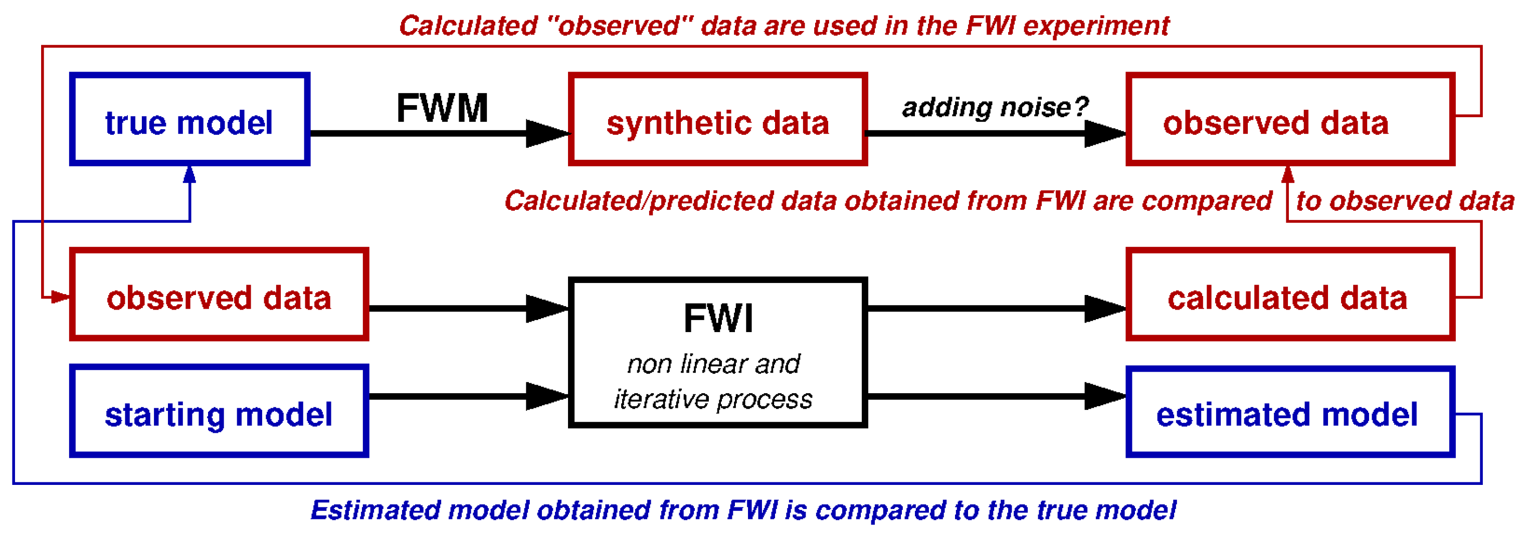
The last step before inversion, is to model the synthetic data according to the geometry acquisition and the source function (type, frequency), and the true model (including the fault) using the FWM (Figure 1). These synthetic data are calculated according to the maximum recording time. This time should be chosen large enough to record the data in the entire receivers including the time where the waves interact with fault. Once the synthetic data are calculated, we can use them as the observed data in the inversion process, directly for free noise experiments, or after adding noise for noisy data experiments.

Finally, we reach the inversion step and so the fault imaging goal. The objective in this step is to use the observed data obtained from the true model and the FWM in the previous step and invert these data to quantify the capability of the FWI for fault detection, delineation and characterization.

The workflow presented in Figure 1 summarizes the main steps during the FWM/FWI process.

3.8. Geological and Physical Models Building and Faults Modelling

In the frame of EGS Alsace project and ANR Cantare programs, a regional 3D structural model was built for Northern Alsace. It is built mainly by reprocessing the old vintage 2D seismic lines [46] which are focused on oil and gas exploration of the Tertiary layers. This geological model could show high uncertainties because at this time, and as the target is shallower than the geothermal reservoir, the used seismic parameters were not adequate to produce images of the underlying crystalline rocks. These uncertainties could mainly be found at the sediments – basement interface which can reach hundreds of meters, especially in the deeper part of the graben, for instance the eastern part. A total of five geological interfaces were modelled and included in this model: (1) “schistes à Poissons”, (2) Tertiary unconformity, (3) top of Trias, (4) top of Muschelkalk and (5) top of Buntsandstein.

In order to build the P- and S-wave velocities as well as the density models from the structural model, we need initial values. For this purpose, we used existing physical, generally 1D, models. These models were obtained from previous studies and from borehole data. These models are good enough for our model building. Once the physical models were chosen, we used them jointly with the stratigraphical 3D model to generate a 3D P-wave, S-wave velocity models and a density model. We defined these parameters in the top and at the bottom of our stratigraphical model, and applied a linear gradient in-between. We show on Figure 2 cross-sections of P-wave and S-wave models and density model extracted from the complete 3D models.

The sources are placed on the topographic surface. The waves propagate down and no reflected and or transmitted waves occur above the surface. As a complete wave field is modelled and the full seismic propagation equation used, several seismic waves have been considered, for instance up and downgoing waves, converted waves and even multiples.

To define the characteristics of the faulted zone, we carefully analysed the available borehole data for the GPK1, 2, 3 and 4 wells. The objective is to define their average thickness and their physical values, i.e., P- and S-wave velocities and density. We showed in Figure 3 the middle part of the GPK1 where we noted the interpreted faulted zones by the red arrows.

During our fault analysis performed on the GPK1 and GPK2 well log data (e.g., Figure 3) we noted that the apparent fault thickness varies between 15 and 80 m. If we consider a dip fault of 75°, which is a realistic value for GPK1 and the closer boreholes [47] we recompute the real fault thickness which varies between 5 and 25 m. More detailed fault and fractures data analysis can be found in Dezayes et al. [29] and Sausse et al. [30].

From the amplitudes, we also computed the amplitude decreases of the P- and S-wave velocities and density values according to the background, i.e., according to the mean values. From the well data of GPK1 and GPK2 (e.g., sonic and neutron density), the values decreased by 10% to 25% for P-wave velocity, between 10% to 20% for S-wave velocity and between 5% to 10% for densities (Figure 3).

Consequently, for our synthetic experiments, we considered an average fault characteristics value of the real values. We consider a fault zone with the following characteristics: (i) the faulted zone thickness is 30 m and (ii) the decrease of the physical values is 20% for the P- and S-wave velocities and 7% for density. We show on Figure 2 the reference physical models from which the fault contrast is computed. These models are the background physical models.

4. Sensitivity Analysis of the Parameters Describing the Acquisition Geometry

We consider an experimental setup which fits as much as possible the real OVSP setup. The sources are located on the Earth’s surface, and the locations of the well-head as well as the well trajectory (where geophones are located) are realistic. In addition, we have used the seismic velocities and the density models extracted from the 3D models.

4.1. Single Shot Problem

We have started our analysis from the FWI results using only one source, located at zero-offset. This numerical experiment helps to understand the resolution power of the FWI. The initial P-wave velocity and S-wave velocity models used as well as the location of the fault are shown in Figure 2 (the density model is not shown). We have used the following acquisition geometry parameters:

▪

The well is vertical;

▪

The source is located at 0 m offset, on the topographic surface (at 175 m MSL), a pressure, Gaussian first derivative and centred at 50 Hz;

▪

The antenna is made of 198 2C geophones located from 550 m depth down to 4500 m and spaced every 20 m;

▪

The observed data are free of noise.

The fault characteristics are:

▪

Vertical fault extension is 2000 m;

▪

Fault cross the well at 3000 m MSL;

▪

Fault dip is 75°;

▪

Fault thickness is 30 m;

▪

Contrasts are −20% for P- and S-wave velocities and −7% for density.

We have also used the algorithmic parameters tuned in Section 3.6. These parameters have been set as follows: (i) FWI performed without polarization, (ii) spatial correlation range is 20 m, (iii) the main frequency is 50 Hz and (iv) without using the inter-correlation between the physical parameters in order to better understand the sensitivity of each parameter separately.

Besides the interest of the single shot problem for the understanding of the FWI method resolution power, we think that it is also remarkably interesting to study this case on a practical point of view. Indeed, due to restricted financial support compared to the oil and gas industry, geothermal project supervisors tend to choose this single-source data acquisition layout. Thus, it is particularly important to quantify the recovered physical fault images especially in the granite geological context.

We compare on Figure 4 seismograms obtained by FW modelling for the model with and without the fault. Recall that this experiment is done without adding noise. If we consider the standard processing, the reflected phase coming from the fault has a slope corresponding to the downgoing field, which leads us to a wrong interpretation. The apparent velocity between the downgoing waves and the reflections arising from the fault are very close, creating an ambiguity in their origin. The FWI method overcomes this problem by dealing with the full wavefield without wave separation.

We show on Figure 5 the inversion result for a zero-offset single-source VSP experiment after 60 iterations. The result is poor. FWI has recovered a small part of the P-wave velocity field but with artefacts mainly in the upper part of the antenna leading to interpretation difficulties. For the S-wave velocity field, FWI has recovered a small section in the lower part of the antenna, but several artefacts can also be observed. For density, as expected, the result is bad, showing that this parameter is weakly sensitive to the fault and cannot resolve it when reflection redundancy is weak. From the one-source shot experiment, we conclude that in the granites and using the described acquisition geometry and the fault characteristics, we cannot image the modelled fault accurately enough for a reliable interpretation.

We understand from this experiment that in the granite geological context, one zero–offset shot is not sufficient to detect, delineate and characterize faults having the described features.

4.2. Multi-Shots Problem

Several synthetic experiments have been performed for different data acquisition geometries (

Table 1. Geometry data acquisition parameters used in the sensitivity study for fault detection, delineation and characterization.

Expe.	Shots	Shot Offsets [km]	Max Offset [km]
1	1	0	0
2	3	−0.5, 0, 0.5	±0.5
3	5	−1, −0.5, 0, 0.5, 1	±1.0
4	7	−1.5, −1, −0.5, 0, 0.5, 1, 1.5	±1.5
5	5	−2, −1, 0, 1, 2	±2.0
6	9	−2, −1.5, −0.5, 0, 0.5, 1, 1.5, 2	±2.0
7	17	−2, −1.75, 1.5, −1.25, −1, −0.75, −0.5, −0.25, 0, 0.25, 0.5, 0.75, 1, 1.25, 1.5, 1.75, 2	±2.0
8	11	−3, −2, −1.5, −1, −0.5, 0, 0.5, 1, 1.5, 2, 3	±3.0
9	13	−4, −3, −2, −1.5, −1, −0.5, 0, 0.5, 1, 1.5, 2, 3, 4	±4.0
10	15	−5, −4, −3, −2, −1.5, −1, −0.5, 0, 0.5, 1, 1.5, 2, 3, 4, 5	±5.0

). The goal is to quantify the effects of (i) the maximum offset, (ii) the number of sources and iii) the intershot distance effect. Experiment 1 is that discussed in the previous section for a one-source problem. The idea is to compare the experiment results, for instance, to compare the results of experiments 5, 6 and 7 to quantify only the effect of the inter-shots, experiments 6 to 9 to quantify only the effect of the maximum offset and experiments 7 to 10 to understand and quantify the effect of the maximum offset.

The objective is to change the number of shots used in the same inversion run as well as the intershot and the maximum offset to quantify the FWI ability for faults’ detection and characterization. For instance, comparing the results of experiments 5, 6 and 7 to quantify only the effect of the inter-shot spacing, which is 1000 m for experiment 5, and 500 and 250 m for 6 and 7, respectively. The maximum offset of 2000 m remains unchanged for these three experiments. We can also compare the results of experiment 6 and 9 to quantify the effect of the maximum offset alone, which is 2000 m for the experiment 6 and 4000 m for experiment 9, where the inter-shot spacing of 500 m remains unchanged around the well.

Experiment 2 used only three shots distant by 500 m, which is the smallest maximum offset used after the single-shot zero-offset experiment. From experiments 2 to 7, we changed and increased the number of shots, the intershot distance as well as the maximum offset to reach a maximum offset of 2000 m. Experiments 7 to 10 will help us to understand and quantify the effect of the maximum offset. In all these experiments, we used the starting physical models shown in Figure 2 and the fault features are those used in the single-shot problem (Section 4.1).

We show in Figure 6 the results summary of experiments 2, 4, 6, 8 and 10, showing the recovered P- and S-wave velocity fields as well as the recovered density model. In Figure 6a, we show the retrieved models for experiment 2 (Table 1) where only three shots are used with a maximum offset of 500 m. The FWI has partly recovered the upper part of the fault in the P-wave field and density but less in the S-wave field. We note that in the P-wave field, the shape of the fault is nearly completely recovered. The physical values remain lower than those of the real model, however. The lower part of the fault is not well resolved for P velocity because beside the direct P, the only phase is the downgoing P-to-S converted wave. We note also that several significant artefacts are present that would lead to wrong geological interpretations.

When we increase the number of shots up to seven and the maximum offset to 1500 m (Table 1 and Figure 6b), the fault is better resolved. The upper part of the fault is better delineated for the three physical parameters. The lower part of the fault remains however not well resolved (better for the S-wave field due to the downgoing P-to-S converted phase). The artefacts remain relatively significant for the three parameters (Figure 6b).

In Figure 6c, we show the retrieved physical models for experiment 6 (Table 1) where nine shots and a maximum offset of 2000 m were used. The retrieved models, compared to experiments 4 and 2, are better resolved, especially for the lower part of the fault. This lower part is less revolved compared to the upper part, and the inverted physical values for the three parameters show underestimated contrasts. We also note the significant improvement of these results, for instance the artefacts present in experiments 1, 2 and 4 are attenuated, except for the density model as expected, because the density is always less resolved then P- and S-wave fields for borehole FWI context.

When increasing the maximum offset to 3000 m (experiment 8) and the number of shots to 11 (Figure 6d), the estimated physical models are improved. These improvements are higher for the P velocity field and the density field than for the S velocity field. Nevertheless, the retrieved density model still exhibits important artefacts.

The last results (Figure 6e) were obtained from experiment 10 (Table 1). The number of shots is 15 and the maximum offset is 5000 m. The fault is accurately retrieved, and the obtained values are compared to those of the real model, except for the lower fault extremity where the values are underestimated. This is mainly true for the P- and S-wave velocity fields, but not for the density. The density model is better recovered except for the area crossing the well, where some artefacts remain visible.

To conclude, the five experiments studied (e.g., experiments 2, 4, 6, 8 and 10) and documented in Table 1 reveal that in the crystalline basement and for a 2D model and seismic modelling):

▪

Three shots allow the detection of the fault but are not enough to delineate the fault and characterisation is not reliable. The delineation is not complete and not precise, and its physical values are different than the real modelled values.

▪

Even when using seven shots, fault delineation is not completely successful if the maximum offset is less than 1500 m.

▪

The fault is well delineated using nine shots or more with the maximum offset of 2000 m or more (to be compared to the target depth, in fact, the rule of thumbs is: maximum offset should be around the target depth).

▪

Increasing the number of shots in the same inversion is not necessarily the best way to go. For instance, the results are improved from experiment 5 to 6 but not between experiments 6 and 7, where the maximum offset of 2 km is the same for both. This means that the included model-part during the inversion which affects really the data is the same for both experiments. Even though the model complexity is the same between these experiments, we improved only the results of experiment 5. We also remember that parameters affecting the data, for instance attenuation, noise level (here free noise), diffractions, etc., are the same.

▪

It is important to make a balance between the number of shots and the maximum offset which should be used to accurately delineate the fault.

▪

The lower part of the fault is always less resolved as the downgoing scattered field has only the converted P-to-S converted wave while the upgoing scattered field is made of two phases, the reflected P-wave and the reflected P-to-S converted wave.

Note that the inter-shot spacing of the experiments discussed above is 500 m, while the number of shots and the maximum offset is varying. The shots at large offsets clearly provide more information through the scattered field. This is not the case with real data as the shots at large offsets exhibit low S/N ratios.

We would like also to quantify the effects of the number of sources for a constant maximum offset. We set the maximum offset to 2000 m and consider various numbers of shots. The number of shots of experiments 5, 6 and 7 (Table 1) are respectively 5, 9 and 17. This means that the inter-shot spacing is different between these experiments, from 1000 m for experiment 5, to 500 m for experiment 6 and down to 250 m for experiment 7.

Slight or non-negligible improvement can be observed between experiments 5 and 6 in all recovered physical parameters. We recovered better the lower part of the fault in experiment 6. This is the direct effect of the number of shots and the intershot distance. Where a non-negligible effect is observed between the results of experiments 5 and 6, no visible effect was observed between the results of experiments 6 and 7. The reason is that for our target, the minimum inter-shot spacing is already reached in experiment 6 and even if we increase the shots number, and decrease the inter-shot distance, the imaging results are not improved. For real noisy data, a smaller inter-shot spacing distance and more sources should be needed, depending strongly on the noise level and the depth of the target. For a real case, a sensitivity analysis could be performed including different noise types and amplitudes to quantify their effect and then choose the optimizing acquisition geometry.

We conclude from these experiments that the number of shots and the inter-shot spacing are both important. It is not appropriate to use several sources with kilometric inter-shot spacing or inter-shot spacings smaller than 250 m (for a 3 km depth target fault and data main frequency of 50 Hz). We observed that using a small number of shots does not allow us to recover accurately our target fault, especially its lower part (e.g., Figure 6a,b), but also that using more shots with non-adequate inter-shot spacing do not improve the results (e.g., experiment 7, Table 1). We should define an appropriate distance from a sensitivity analysis, which could change according to the depth, thickness, dip, azimuth, and so on, of the target. According to the faults which could be met in the granite of Soultz-sous-Forêts, the best parameters deduced from the sensitivity study are: (i) the optimized number of shots is 9, (ii) the intershot distance is 800 m, and (iii) the maximum offset is 4000 m.

We recall also that these conclusions hold for noise-free data and for a 2D seismic modelling. For noisy data, the number of required shots would increase. And for a 3D model with azimuth coverage, the number of necessary shots N should be around $\pi n^2/4$, where n is the number of shots needed for 2D.

5. Sensitivity Analysis of the Fault Parameters

We now use the best acquisition geometry parameters determined in the previous section and study the seismic effect of the fault features: (i) the fault geometry (length, dip, distance from the receiver) and (ii) the fault physical characteristics (P- and S-wave velocities, density contrasts and thickness). The thickness of the fault zone is a geometrical parameter but as this parameter is related to the ability of the FWI to retrieve the true values of the physical parameters inside the fault zone, we consider it as a physical parameter. The ability to retrieve the true values of the physical parameters (fault characterisation) is also related to the main frequency of the seismic data.

5.1. Fault Geometry Parameters

We consider a fault with the same features as that described in the single-shot problem (Section 4.1). We vary the fault dip (0°, 30°, 60°, 75°, −75° and 90°)) and the fault distance from the well: fault crossing the well, or horizontally shifted by 600 m or 1000 m from (Figure 7). The same inversion parameters were used: 20 m for the spatial correlation length, and without polarization. Concerning the correlation between the physical parameters contrasts, Vp, Vs and density, we consider two cases: (i) a strong correlation, i.e., crosscorrelation coefficients of 0.9 for the three couples of parameters) and (ii) a moderate to strong correlation, i.e., 0.8 for the (Vp, Vs) couple and 0.6 for the two other couples (Vp, density) and (Vs, density). We used the best geometrical data acquisition recovered in the previous sensitivity study (Section 5.2), namely (i) 800 m for the inter-shot spacing, (ii) maximum offset of 4000 m, and (iii) eleven shots located at the following offsets: −4000, −3200, −2400, −1600, −800, 0, 800, 1600, 2400, 3200 and 4000 m (Figure 7).

We have summarized in Figure 8 the sensitivity to fault dips for the faults crossing the well and the receivers. We can observe that the fault dip is not an issue even at high dips (>75°). Generally, the higher the fault dips the better the FWI retrieves the whole fault shape and contrasts. This is true except for a horizontal fault, where the fault parts close to the receivers are accurately recovered, but not the faraway parts (Figure 8d). Nevertheless, the physical parameters for the parts closest to the receivers are accurately recovered. We note that for high dip faults, i.e., >60° (Figure 8a,b), we recovered accurately the entire upper part of the fault, but not completely the lower part, as in the previous experiments (see Section 5). This is due to the scattered field, as already explained. The worst cases are for shallow dipping faults, probably between 10° to 40° more or less (e.g., Figure 8c). We note also the presence of some artefacts in the recovered density field, but again we can observe that for a horizontal fault (Figure 8d) and for high dip faults (e.g., Figure 8a), the retrieved density field is better than the retrieved P- and S-wave velocity field.

In a second step, we have considered the case of the distance of the fault from the well. What is the maximum distance where a fault could be accurately imaged or even detected? The results of the FWI for the faults 2, 3 and 5 are shown in Figure 9 and for the faults 7 and 8, in Figure 10. The FWI can accurately detect and delineate the fault even when it is far away from the receivers. The maximum distance varies from 500 m for the lower part of the fault to 1000 m for the upper part (e.g., Figure 9). This maximum distance decreases when the dip decreases. When the fault dip decreases from 75° to 60°, the farthest part of the fault is not detected (compare Figure 9a,c). When the fault dip decreases, we delineate with more accuracy the closest part than the furthest part, this can be noticed when comparing faults 2 and 5. This is expected, because when increasing the fault dip, we increase the distance between the upper part of the fault and the receivers, for the same fault length. We note also that the density field is recovered with some artefacts, and its physical values were recovered accurately. We recall that the inverted data are free of noise, and we expect these maximum distances to be smaller with real noisy data.

The conclusions of the previous section concerning the fault dip remain true. We observed that the higher the fault dips, the better we can delineate the fault and recover the contrasts in the physical parameters. This is the case even for a vertical fault (Figure 10b). In this case, the fault is accurately delineated, and the P-wave velocity and the density fields are recovered with a good precision. The S-wave velocity field show a correct delineation, but the contrasts are not well estimated in the deeper part of the fault. The reason is that in this part, the P-to-S reflected (from right side sources), or the transmitted converted S waves (from left side sources) provide information only at a few receivers (the deepest). Even for a vertical fault, the FWI shows a high potential to accurately recover its shape and the physical contrasts, which is not the case to the classical VSP processing approach (see discussion below).

The challenging fault shape is for a dip of −75° when the fault is far away from the receivers and when reflected waves cannot reach the receivers. We can notice that for the P-wave velocity field (Figure 10a), only a small upper part is recovered, whereas for both the S-wave velocity and density fields, the whole fault is correctly delineated, but with underestimated contrasts. The S-wave velocity field is better estimated due to the P-to-S converted waves of the scattered field (Figure 11). Notice that in the well vicinity (distance less than 300 m) the FWI has accurately recovered the shape and the physical contrasts of the fault. The tendency is that the physical parameter contrasts are more underestimated when moving down and away from the well.

An interesting comparison could be made between the FWI technique and the standard OVSP data processing technique for their ability to detect and characterize faults in the granites. This sensitivity study shows us that we can fairly to accurately detect, delineate, and characterize fault zones in the granite context (in the well vicinity). Experiments show also that the higher the fault dip, the better is the fault delineation and also the better we characterize the physical parameter contrasts. A standard approach, where OVSP data are processed classically by separating the recorded field to up- and down- going fields and where only the first seismic order (primaries) of the upgoing fields is used, would fail for faults with high dips. Reiser et al. [10] obtained accurate fault imaging for faults, especially those with a shallow dip, and demonstrated that the Kirchhoff migration cannot provide accurate fault imaging for high fault dips: the faults dipping at 30° are, for instance, better imaged than those at 70° (also in a granite context). The authors have also noted the presence of important artefacts that cannot be removed even when they increase the source number due to the diffraction hyperbola. For the FWI method, the most challenging fault dip could be found for dip angles of 10–40°. For fault dips between 45 and 90°, which are the most frequently found in deep geothermal crystalline contexts, the FWI show a fully accurate fault imaging result. Very few faults may present this maximum dip (i.e., 90°), but the idea here is to check the ability of the applied method in very steepest contrasts. Additionally, the observed artefacts are removed when increasing the number of shots to seven, and completely removed with nine shots, because the multiple diffractions or high order scattered field constitutes useful information. In other words, as the full wave equation reproduces these phases, we can invert this part of the wavefield, introducing constraining information and helping the inversion to provide an accurate and realistic underground image. However, we recall that these FWI synthetic experiments have been performed for perfect data (noise free) and for a 2D world (i.e., the fault is always perpendicular to the propagation plane). We recall also that the aim of this study is to demonstrate the ability of the FWI to recover accurately faults with realistic parameters and characteristics, besides the real data complications (for instance attenuation, 3D effects, alterations and anthropogenic noise) which could not affect considerably the results of this study, because their effects (e.g., attenuation) do not play a major role in the FWI.

We have performed an additional sensitivity study regarding antennae length. We have found as expected that we recover only the fault part located at the receiver depths. This means that when a fault is detected and delineated, its length could not be the complete length if the recovered fault length and the antennae are comparable.

The sensitivity analyses described and discussed above have been performed for a fault thickness of 30 m. What is the minimum fault thickness which can be recovered in the granites using the FWI technique? Even if the thickness is a geometrical parameter of the fault, its estimation is related to the physical parameter contrasts and the frequency content of the seismic signal (interaction between the wavelength of the P- and the S-wave and the fault thickness); this is why we have considered this parameter separately.

5.2. The Fault Thickness Issue

We start by analysing the quantitative parameters recovered in the previous experiments. For instance, we focus on the horizontal profile of the estimated physical parameters for fault no. 4 (see Table 1, Figure 8b), which represent a fault crossing the well at 3000 m, showing a dip of 60°, a thickness of 30 m and 20, 20 and 7% for P- and S-wave velocity and density contrasts, respectively. Qualitatively, remember that the upper part of this fault was accurately imaged by the three parameters (i.e., P-, S-waves and density), but its lower section was partly imaged. The contrast analysis (Figure 12) provides a quantitative view. The fault contrasts in its upper part before crossing the well is fully recovered where at least 97% of the maximum contrast is retrieved. Some oscillations can be observed for the density.

The physical parameter contrasts for the lower part of the fault are poorly recovered in the P-wave velocity field where 400 m below the receivers (i.e., at 3400 m depth), only 40% of the maximum contrast has been recovered (Figure 12d), whereas 70% of the S–wave contrast has been obtained, and an overestimation of 120% for the density. Considering the lower fault extremity (Figure 12e), less than 10% of the P-wave velocity contrast has been retrieved and around 45% for the S-wave velocity and 75% for the density. Note that the density provides better results for free noise data, and it is more sensitive to noise as the obtained results quality decreases when increasing the noise (Figure 12).

To quantitatively address the fault thickness, we consider the geometry data acquisition as that shown in Figure 7, and we consider the fault (1), dip of 75° with different thicknesses. We have studied the following fault thicknesses: 5, 10, 15, 20, 30 and 50 m. Both acquisition geometry and inversion parameters remain unchanged, for comparison with the previous images obtained for a fault thickness of 30 m.

We can notice that the fault contrasts have been accurately estimated by the FWI (Figure 13). Qualitatively, the fault has been accurately retrieved in all experiments. The fault location was rightly estimated, even for the very narrow fault of 5 m thickness. It is also important to quantitatively assess the FWI estimated contrasts especially for narrow faults, i.e., fault thickness less than 20 m (see discussion below).

In the granite, the P-wave velocity value is around 6000 m/s as showed by sonic logs acquired in GPK1 borehole (e.g., [48]. For a central frequency of 50 Hz, as is the case for our experiments, the seismic wavelength for P-waves is 120 m (i.e., λ = 120 m) and about half for the S-wave (70 m). Barnes and Charara [13] show that for OVSP data, when the scattered S-wave field is energetic (as often when offset is sufficient), the S-wave velocity estimated field provides a better spatial resolution than the P-wave velocity field, even when S-wave suffer from seismic attenuation because the scattered S-wave field is mainly generated in the well vicinity implying small propagation distances. Moreover, and because it deals with the complete wave equation, the FWI can detect and delineate faults even for thicknesses of λ/10 (i.e., for λp = 12 m, and λs = 7 m). In a sedimentary context, thin beds can also be detected with thicknesses of λ/1 [13] However, as the scattered energy decreases with the fault thickness, in the real world, the scattered energy from a thin fault can easily be covered by ambient noise. Therefore, for real data, the detection, delineation, and characterization of thin faults depend strongly on the data quality and on the S/N ratio.

As the seismic wavelength is around 120 m (70 m for S-waves), we observe also that either for faults of 5, 10 and 15 m thick (Figure 13a–c), we accurately recovered their locations and dips, but what about the recovered contrasts?

The obtained contrasts compared to the true contrasts are shown on Figure 14 for several experiments, including different fault thicknesses (5, 10, 15, 30 and 50 m) and at a particular depth of 3000 m. It was clear that the FWI will provide precise faults geometries and their characteristics, i.e., velocities and density contrasts, for thick faults (>30 m). Contrasts of these thick faults have been accurately retrieved, especially for P- and S-wave fields but less resolved for density fields, with some artefacts (Figure 14e,f). Surprisingly, precise contrasts have been recovered for very narrow faults of 5 and 10 m (Figure 14a,b). When comparing the FWI estimated contrasts to the true contrasts (Figure 14), precise values have been obtained for all thicknesses (

Table 2. The recovered contrast according to the maximum true contrasts, where True means the physical parameter contrast for the fault in the reference or True model and FWI means the physical parameter contrast for the fault in the models estimated by the FWI. Note that these contrasts are relative to the background values.

Fault Thickness [m]	P-Wave Velocity Contrast [m·s−1]		S-Wave Velocity Contrast [m·s−1]		Density Contrast [kg·m−3]
	True	FWI	True	FWI	True	FWI
50	−1031	−1089	−557	−492	−135	−189
30	−972	−839	−525	−456	−128	−188
20	−778	−603	−421	−327	−102	−141
15	−635	−501	−343	−279	−83	−64
10	−443	−373	−240	−203	−58	−78
5	−238	−198	−129	−111	−31	−34

), where the worst recovered contrast is 97% of the maximum true contrast, which is very satisfactory for fault thickness characterization, especially for narrow faults (i.e., fault thickness less than 15 m).

5.3. The Multi-Faults Experiment

We now consider four faults with different lengths and thicknesses, and a deviated well. We thus mix different challenges in the same inversion experiment to explore the ability of the FWI method to separate and interpret the scattered fields of the different faults. The modelled fault features are shown in

Table 3. Fault features of the multi-fault experiment. The VC. Stand the Velocity Contrast (idem to C). The fault locations are shown in Figure 15.

Features	Faults
	a	b	c	d
Thickness [m]	20	50	25	40
Dip [°]	−60	−60	75	80
P-wave VC. [%]	25	20	25	20
S-wave VC. [%]	25	20	25	20
Density C. [%]	10	7	10	7

. The faults a, c and d cross the well, whereas fault b is located in the vicinity of the well at the right side, under the receivers.

For acquisition geometry parameters, a total of 21 sources have been used with increasing inter-shot spacing from 250 m, around the well, to 500 m at intermediate distance (between 1 and 3 km away) to reach 1000 m at large offsets. The maxim offset used is 5000 m. The deviated well is inspired by GPK4 at Soultz-sous-Forêts. We do not add noise. The obtained P- and S-wave velocity and density estimated fields are shown in Figure 15 after 100 iterations. The FWI accurately recovers the fault locations and their shapes except for the deepest part of the faults c and d, as was observed in the previous experiments. These deep parts are better recovered for the S-wave estimated field than for the P-wave field and density as in previous experiments.

From the estimated fields, we can observe that the most important parameters affecting the results are the dip and location of the faults according to the receivers (Figure 15). We also notice that even if the fault does not cross the well, the FWI can retrieve accurately the fault characteristics. From the P-wave velocity estimated field, we can notice that the fault b is better resolved, then d, then c and finally a. The major difference between the resulted fault features for fault a and b, which have the same dip, is mainly their thickness, where the fault b thickness is 50 m, and only 20 m for fault a (Table 3).

The main result from the multi-fault experiment is that (i) the overall conclusions are the same as for previous synthetic FWI experiments and (ii) the presence of several faults does not affect the accuracy of results for each fault independently, at least in 2D and using noise-free data. In addition, we have understood from this experiment, that the FWI can provide a clear underground image of faults network, at least for fault zones having average characteristic values as those modelled here. For instance, fault a, which is only 20 m thick, is recovered in the right location and shape, but its thickness is underestimated. Undoubtedly, the narrow faults, typically with a thickness of less than 20 m, will be more challenging.

During the FWM, we can record the waves’ propagations through the entire experiment. Figure 16 shows snapshots at times 2 ms, 660 ms, 850 ms and 1050 ms. The P- and S-wave front can be followed and their interactions with the faults are visible. P-to-S and S-to-P wave conversions are also visible. Combining these screen shots, we built a movie (see the Supplementary Material to watch it). Analysing continuously the seismograms and the movie, we better understand the different phases in the seismograms and their origins.

6. Results and Discussion on the FWI Robustness for Noisy Data

In order to demonstrate the FWI ability for fault delineation and characterization, it is important to separate the data quality issue (information content of the data) and the starting model issue (non-linearity) from the imaging issue. This is why we have performed sensitivity analyses using noise-free data in the above sections (even the numerical noise is negligible as it is the same in the observed data and in the calculated data). We now test the FWI performance with moderate and high noise in the data using experiment 5 as a reference (Table 1). We considered the noise with the following characteristics:

▪

Additive Gaussian noise,

▪

Noise has the same f-k amplitude spectrum than the data,

▪

Ambient noise is unlocalized,

▪

Coda noise is localized a few periods after energetic phases.

We show in Figure 17 the Z-components for the three experiments namely Ref, MN and HN (

Table 4. The two noise parameters, ambient and coda, used in the noise study. The reference experiment is experiment 5 (Table 1).

N/S Amplitude Radio	Ambient [%]	Coda [%]
Noise free (Ref)	0	0
Moderate noise (MN)	15	25
High noise (HN)	30	50

). We can observe that for free noise data, we identify clearly the arrivals crossing the first arrival from −2000 m, whereas in MN these arrivals are more difficult to identify. For HN, these arrivals cannot be identified. We focus on these arrivals, because they are generated from our target (i.e., the fault).

We have run the FWI for these three experiments, as shown in Figure 2. The outcomes are shown in Figure 18. As expected, the estimated fields are noisy. The FWI detects the fault and retrieve quite accurately the shape and the location of the fault as well as its dip, even for noisy data (e.g., Figure 18b). The contrasts in the physical parameter are not well estimated. As previously observed, the lower part of the fault is partly recovered for both the P- and the S-wave velocity fields. This is due to the short maximum offset used in these experiments (2000 m) which is less than the optimal one (4000 m). Several artefacts can also be observed implying ambiguities in the interpretation (e.g., Figure 18c).

For the case of the moderate noise experiment (MN), the FWI is able to provide an accurate fault detection, delineation, and characterization (Figure 18b).

In the high-noise experiment (HN, Figure 18c), the upper part of the fault in the P-wave velocity field is recovered, but it is less well defined in the S-wave velocity field (and not well retrieved in density field, not shown here). The lower part of the fault is recovered partially in the P- and S-wave velocity fields, the delineation can be obtained but not the physical parameter contrasts. This HN experiment illustrates the capability of the FWI to detect and delineate faults, even for noisy data in the granite context. We recall here that this noise, even high, is structured, additive and Gaussian, which is theoretically compatible with the least square method used in the FWI. The application to real data is not as straightforward as in a sedimentary context. Effectively, the FWI needs a precise starting model including a complex rheology in order to account for the main heterogeneities (structures), the travel times of the main downgoing waves, and potentially, anisotropy or attenuation effects in the data. Some experiment parameters have to be inverted (as the source function for instance). Finally, the noise characteristics, depending on the dataset, should be carefully studied as the seismic data quality is always a key issue when using the FWI technique. All these issues have been already addressed with success in sedimentary contexts for oil and gas applications. The present results prepare the application of the FWI method to real borehole data in a crystalline basement and we hope that they will ease the interpretation of its outcomes.

7. Conclusions

We have performed several sensitivity analyses of the full wave inversion (FWI) method using numerical full wave modelling (FWM) in order to assess the capabilities of the FWI method for the purpose of detection, delineation, and characterization of faults in a crystalline basement. By adopting the following simplifications, we are somehow assessing the maximum capabilities of the FWI:

▪

Seismic modelling is performed in 2D using an elastic isotropic rheology. We do not address the attenuation and anisotropy issues. 2D modelling implies that the propagation plane is parallel to the dip direction of faults, therefore, the azimuthal dependency of the inversion results is not addressed (this would require 3D modelling).

▪

The starting model issue is not addressed.

▪

The acquisition geometry and experimental parameters for the source and receivers are perfectly known.

Most of the experiments are performed using noise-free data, i.e., perfect data. This allows us to check the method independently of the noise characteristics, i.e., the capabilities of the FWI methods when data conditions are perfect.

We have studied several sets of parameters: (i) the inversion algorithmic parameters for the crystalline basement context, (ii) the acquisition geometry parameters, and (iii) the fault characteristics parameters. For algorithmic parameters, the goal was to tune the inversion process in the FWI in order to optimize the results, and improve the final quality of the recovered underground images (i.e., the physical estimated fields). For instance, and contrary to sedimentary contexts, considering the data polarization increases the artefacts in the estimated fields. We have also tested several spatial correlation ranges. We have found that a range of 20 m, i.e., a little less than the fault thickness, yields the best results according to the thickness of the fault target. We have also tested the crosscorrelation between the P-, the S-wave velocities and the density parameters as strong positive correlations are noticeable in well logs, and we have found that the obtained images are improved, and the artefacts are clearly attenuated.

In the second step, we have studied the effect of the acquisition geometry: (i) the number of shots, (ii) the inter-shot distance and (iii) the maximum offset, which could be used to improve the final FWI results. Using a single shot in the granite is more challenging for the FWI to accurately characterize the fault. The presence of important artefacts in the estimated fields creates ambiguities in the interpretation of the fault images. As expected, these artefacts are attenuated when increasing the number of shots. With three shots, the quality of the retrieved images is improved but the estimated fields remain perturbed by artefacts. With five shots, we obtain better estimated fields and from seven shots and up, we accurately retrieve the fault with negligible artefacts. For a given number of shots, small inter-shot spacing (around 250 m) and large inter-shot spacing (around 1000 m) do not give suitable results. A reasonable intershot distance should be defined according to the depth of the target and to the seismic main frequency. Shots at far offsets (once to twice the target depth) provide constraining information to the FWI method. However, the quality of real, noisy data at far offsets is often not sufficient. The optimal acquisition geometry parameters depend on the S/N ratio. Of course, these conclusions have to be adapted when considering a 3D domain.

Considering the fault delineation and characterization goals, we studied the effect of the fault thickness and its dip in both configurations: a fault crossing the receivers in the well, and a fault far away from the well. The obtained spatial resolution is good even for a very thin fault of 5 m, where about 98% of the physical parameter contrasts have been recovered. This result stands for noise-free data but, as the energy of the scattered field decreases with the fault thickness, the S/N ratio is critical for thin fault zones. We can accurately detect, delineate and characterize faults with high dips (60° to 90°). Horizontal faults and their features were also retrieved accurately. The dips ranging between 10 and 40° remain a challenge. This may not be a critical problem because this fault dip range seems uncommon in granite, judging by the Soultz-sous-Forêts and Rittershoffen geothermal sites (e.g., [26,27,29]. The multi-faults case was also studied and the FWI showed a noticeable robustness and ability for delineation and characterization objectives. The delineation and characterization of a fault network could be considered in future applications. This capability of the FWI method has to be investigated further, especially in 3D, by studying the azimuthal effect for noisy OVSP data.

For a moderate noisy data, the FWI showed a high potential to detect, delineate and even characterize faults in the crystalline context. This opens new perspective for its future application on real data.