Abstract
Geological contexts that lack minimal stratigraphic and piezometric information can be challenging to produce an initial hydrogeological map in remote territories. This study proposes an approach to characterize a regional aquifer using transient electromagnetic (TEM) surveys. Given the presence of randomly dispersed boreholes, the Saint-Narcisse moraine in the Mauricie region of Quebec (Canada) is an appropriate site for collecting the required geophysical data, correlating the stratigraphic and piezometric information, and characterizing regional granular aquifers in terms of stratigraphy, geometry, thickness, and extent. In order to use all TEM results (i.e., 47 stations) acquired in the moraine area, we also correlated 13 TEM stations, 7 boreholes, and 6 stratigraphic cross-sections to derive an empirical and local petrophysical relationship and to establish a calibration chart of the sediments. Our TEM data, combined with piezometric mapping and the sedimentary records from boreholes and stratigraphic cross-sections, revealed the compartmentalization of a multi-kilometer morainic system and indicated the presence of two large unconfined granular aquifers overlying the bedrock. These aquifers extend more than 12 km east to west across the study area and are between 25 and >94 m thick. The TEM method provides critical information on groundwater at a regional scale by acquiring information from multiple stations within a short time span to a degree not possible with other existing methodologies.
1. Introduction
Morainic complexes have a spatial arrangement and hydraulic characteristics (i.e., permeability, porosity, and particle size) that are favorable for groundwater storage [1,2]. Often located in northern environments and far from urban areas, moraines are sometimes difficult to access, and collecting data using conventional hydrogeological methods, such as boreholes and piezometers, can be challenging in these environments. Geophysical surveys can quickly investigate an accumulation of glacial sediments (e.g., a moraine) to efficaciously assess the internal dimensions and stratigraphic variability of any contained aquifers. The transient electromagnetic (TEM) method applied to groundwater exploration provides a non-invasive, inexpensive, and effective means of characterizing the internal structure of moraine deposits and delineating the geometrical features of various hydrogeological targets [3,4,5].
In the province of Quebec, Canada, the deglacial period saw the formation of complex granular aquifers, such as those associated with the Saint-Narcisse morainic complex. This deposit is a major Quaternary formation that stretches along the southern margin of the Canadian Shield and extends from the town of Saint-Siméon in Quebec to the Great Lakes in Ontario [6,7]. This vestige of the Younger Dryas cooling period (12.7–12.4 cal. ka BP; [7,8]) was deposited during a readvance of the Laurentide ice sheet (LIS). Thick layers of well-sorted sands and gravels have been observed at the surface of this morainic complex [6,7,9,10]; these deposits represent potential aquifers. The overall extent of the Saint-Narcisse morainic complex is not continuous and is frequently interrupted by multiple sections composed of finer sediments deposited by the Champlain Sea [6] during its incursion into the isostatically depressed region following the retreat of the LIS. These less permeable sediments (i.e., clay and silt) act as natural impermeable barriers that limit connections between granular aquifers, create a discontinuity of the stratigraphic units within the moraine, and compartmentalize any contained aquifers.
In the Mauricie region of Quebec, Canada (Figure 1), municipalities have collected hydrogeological data (e.g., borehole logs, pumping tests, and piezometric surveys) from around the moraine. Nonetheless, the distribution of these aquifers remains poorly constrained and documented, and no study has yet to investigate their spatial extent, thickness, and location. Furthermore, the existing groundwater-related data have never been integrated into a regional-scale portrait of these morainic aquifers. The Saint-Narcisse morainic complex is mainly located in rural areas, and several sectors of the moraine are difficult to access and are thus characterized by a lack of data. Here, we aim to improve the existing stratigraphic data by establishing: (1) the simplified architecture of the deposits; (2) the groundwater elevation; and (3) the depth of the bedrock.
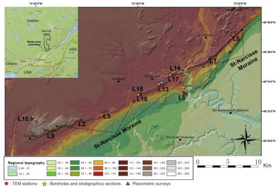
Figure 1.
Regional topography of the study area and location of TEM 2D sections, boreholes, stratigraphic cross-sections, and piezometric surveys acquired from the Saint-Narcisse moraine.
The electrical resistivity values of the Saint-Narcisse moraine deposits are unknown, and establishing a correlation between the stratigraphy and the geophysical response is not straightforward [11]. Several authors [12,13,14,15,16,17] have shown that different subsurface sedimentary layers can share a similar resistivity; therefore, there can be a possible overlap between different stratigraphic units and electrical resistivity values. To circumvent this overlap problem and efficaciously use the TEM approach, we develop, in an initial step, a calibration chart of electrical resistivity values associated with each sediment class typically found within the Saint-Narcisse moraine in the Mauricie region. This chart allows for the interpretation of the obtained electrical resistivity values for both unsaturated and saturated sediments. The chart also extends the interpretation of TEM results collected during the field campaign to locations where no boreholes or piezometric observations are available (i.e., 27 stations). To characterize the Saint-Narcisse morainic aquifers at a regional scale, we then use TEM to collect geophysical data in support of hydrogeological mapping to (1) improve the understanding of the sediment architecture within the moraine and (2) delineate the spatial extent of the Saint-Narcisse moraine aquifers in the Mauricie region. This study was conducted in 2019–2020 as part of the Groundwater Knowledge Acquisition Program (PACES; [18,19,20]), sponsored by the Quebec Ministry of the Environment (MDDELCC). The various PACES projects aim to produce a realistic portrait of existing groundwater resources of the municipalized territories of southern Quebec to protect these aquifers and ensure their long-term sustainability.
2. Study Area and Geological Overview
2.1. Basement Geology
The study area is in the southeastern portion of the Mauricie region, situated between Montreal and Quebec City (Figure 1). This area, lying between the St. Lawrence Lowlands and the Grenville Province, consists mainly of a relatively flat topography where agriculture is the main economic activity. The St. Lawrence Platform (i.e., St. Lawrence Lowlands) lies to the south of the moraine and is composed of Paleozoic sedimentary rocks, which are covered by a thick layer of Quaternary sediments. These sedimentary rocks are composed mainly of Ordovician sandstone (Black River group), carbonate (Trenton group), and shales (Utica and Lorraine groups) deposited in a marine environment [9,11,21,22]. This geological province is bounded to the northwest by the Precambrian Canadian Shield and to the southeast by the Appalachians. The Grenville Province, the youngest province of this Precambrian shield, lies to the north of the study area and consists mainly of high-grade igneous and metamorphic intrusive rocks [23]. The lithologic composition of the Grenville Province varies depending on the area; anorthosite, mangerite, charnockite, orthogneiss, paragneiss, migmatite, and marble are the main rocks found near the study area [11,22,24].
2.2. Quaternary Sediment Deposits
Quaternary surface deposits in the Mauricie region (Figure 2) were mapped recently under the 2018–2021 PACES project directed by the University of Quebec at Chicoutimi (UQAC). Most Quaternary deposits associated with the Saint-Narcisse moraine relate to the last glaciation (i.e., Wisconsinan glaciation) and were deposited during deglaciation. The isostatic depression caused by the LIS, combined with a rapid global rise in sea level, led to a marine transgression and the incursion of the Champlain Sea into the region. The sea flooded the valleys of the lowlands and led to deposits reflecting both deep and shallow marine environments (i.e., distal and proximal glaciomarine deposits) in the study area. This marine transgression lasted about 2000 years (13–11.2 cal. ka BP) and reached an elevation of about 200 m asl (i.e., above present-day sea level; [25,26]). Isostatic rebound during the Holocene provoked a marine regression, and the Champlain Sea deposited regressive sands during its retreat.
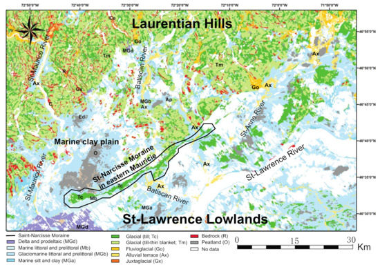
Figure 2.
Surface deposit map of Quaternary sediments from the southeastern Mauricie region. The four main hydrogeological contexts are identified: Laurentian Mountains, marine clay, Saint-Narcisse moraine, and St. Lawrence Lowlands.
Saint-Narcisse Moraine
During the last glacial period, the LIS covered most of Canada and attained a thickness of 5 km in places [27,28,29,30,31,32,33]. This ice sheet crushed, removed, and transported rocks and sediments and produced glacial deposits composed mainly of diamicton (i.e., tills). Climate-related phases of LIS advance and retreat left behind numerous frontal moraines represented by long ridges composed of glacial sediments [32,33,34]. The Saint-Narcisse morainic complex is discontinuous but extends over more than 1400 km and is one of the longest documented frontal moraines in Canada [6]. The moraine can reach up to 100 m thick, although it generally varies locally between 1 and 20 m [9,35]. A variety of sedimentary facies make up the stratigraphic sections of this moraine: till wedges, subglacial or melt-out till deposited during the last glaciation, proximal and distal glaciomarine deposits, as well as juxtaglacial and fluvioglacial deposits (i.e., ice-marginal outwash [7,9]).
In low-lying areas, the Champlain Sea event deposited a thick layer of clay covered by regressive sands deposited during the marine regression. At higher elevations (e.g., the sides and top of the moraine), the Champlain Sea deposited proximal glaciomarine sediments and reworked the glacial tills put in place during deglaciation or the Younger Dryas readvance (YG; [6,7,25,26]). The till deposits were reworked by waves and currents to form visible terraces on the seaward side of the moraine (Figure 1 and Figure 2). Therefore, these terraces are essentially composed of coastal and sublittoral sands deposited in the shallowest areas of the Champlain Sea and by fluvioglacial sediments of small and large deltas that formed in the valleys at the mouths of rivers entering the Champlain Sea [7,8,11,26].
Groundwater found in these areas is the main source of drinking water and is exploited locally to supply several municipalities (e.g., Saint-Narcisse, Saint-Prosper, and Saint-Maurice), which attests to the local aquifer capacity of the moraine. It is therefore possible to deduce that there is likely a high groundwater potential in this area of the Saint-Narcisse morainic complex. Our goal is to validate this potential and delimit the aquifer’s boundaries.
3. Materials and Methods
3.1. TEM Field Setup
TEM measurements are performed using loops of electrical wire deployed on the ground. A time-varying current is injected into a transmitter loop (Tx), which induces a primary electromagnetic field into the subsoil. This initial electromagnetic field interacts with the subsurface geological materials to produce an electric current that induces a secondary electromagnetic field; this secondary field contains information regarding the underground electrical properties and is detected by a receiving loop (Rx) on the surface connected to a receptor that measures the rate of decay of the electromagnetic field. The rate of decrease is then reversed in electrical resistivity [36,37]. This method does not involve direct electrical contact with the ground (i.e., electrodes) and produces results for a range of depths, from a few to several hundred meters. The advantages of this method are numerous. It is inexpensive, non-destructive, fast, robust, and ensures efficient operations within various environmental conditions (e.g., swamps, coastal areas, forests, and mountains; [38,39,40,41]). On the other hand, it has the disadvantage of being sensitive to proximity interference (buried or not), such as the presence of metal pipes, cables, fences, and power lines [14,15].
For this study, TEM data were collected over three months (summer 2020) and involved 47 TEM surveys acquired at 12 locations across the Saint-Narcisse moraine in the Mauricie region. The TEM instrument used for this study consisted of an NT-32 transmitter and a 32II multifunction GDP-receiver [42] and included a portable battery-operated transmitter-receiver (TX-RX) console. For this series of soundings, we used a square-sized loop configuration of 20 × 20 m for the TEM transmitter. The pulse current in the generating loop was set at 3A, and the frequency of the filter was set at 32 Hz with a 50% duty cycle. The turn-off time was 1.5 μs with the damping resistor set at 250 Ω. The induced voltage was measured using a 5 × 5 m receiver loop (in-loop configuration). The NanoTEM equipment consisted of a high-speed sampling card with a fixed gain stage of Å~10. Data were stacked in 8 blocks of 4096 cycles each, giving a total of 32,768 stacks. This resulted in a noise level of approximately 10 μV/A.
3.2. TEM Data Inversion
Once the resistivity data were acquired, our main goal was to deduce the subsurface resistivity distribution by inverting the data. Converting the TEM signals into an electrical resistivity model of the ground involves three processing steps relying on different software packages. First, raw data are averaged using TEMAVG Zonge software [42,43]. This step also filters inconsistent data points (i.e., outliers), which must be deleted before the inversion (Figure 3). Because the magnetic field intensity decreases with depth, the amplitude of the measured data decreases over time, with time playing the role of pseudo-depth. Here, the results are represented by a variation of the apparent resistivity. When the noise level (distortion) increases and the decay rate of the signal becomes discontinuous, the variations of the induced voltage (i.e., dB/dt) increase greatly, and the obtained results are no longer reliable. It is therefore necessary to remove these inconsistent data points (i.e., outliers; red crosses on Figure 3) manually when processing data with TEMAVG to retain only high-quality data. Figure 3 provides an overview of the acquired data and shows measured raw data (as crosses), the residual number, the inversion best fit (black line), and the corresponding resistivity model.
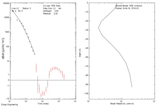
Figure 3.
(Left) Typical induced voltage decay from Line 2 (L2), Station 3. Measured data are shown as crosses and inversion fitting as a black line. The noise level is approximately 25 μV/A. The inversion residual is 2.2. (Right) The obtained smooth-model TEM inversion.
STEMINV software [42] is used for inversion in order to develop a 1D inversion model of the transient EM sounding curves. After importing the data file containing the measured sounding curve from TEMAVG, we used the software to generates a consistent 1D smoothed inversion model of electrical resistivity versus depth on the basis of the iterative Occam inversion scheme [44]. Calculations of maximum depth are given in the Zonge manual [42]. We used MODSECT software [42] for the final phase of data processing to build a 2D model by using the 1D resistivity model acquired with STEMINV [43]. MODSECT interpolates vertical columns with Catmul–Rom splines and then interpolates across the model with splines to provide a 2D view from 1D data in order to visualize the geometry of the geoelectrical structure of each line (Figure 4).
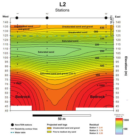
Figure 4.
The interpreted 2D Section L2 and stratigraphic cross-section YL071 taken near Notre-Dame-du-Mont-Carmel, Quebec. The surface deposit elevation is obtained from lidar data. The blue dashed line represents the projected water table from direct observations in the field. The legend indicates only those sediments observed directly in the area (YL071). If no boreholes (or stratigraphic cross-sections) were acquired, the subsurface information is deduced from the calibration chart.
3.3. TEM Calibration
Indirect geophysical methods are a necessary complement to direct observations obtained through borehole logs, stratigraphic cross-sections, and piezometric surveys. These direct measurements are used to calibrate the geophysical results, thereby allowing the extrapolation of all TEM results (i.e., 40 stations) over a larger study area, even for areas lacking nearby sites where data were acquired directly. This calibration involves comparing the stratigraphic and piezometric information with the TEM results to obtain an equivalence of the electrical resistivity values for the unsaturated and saturated sediments of the study area. We selected TEM stations (1D resistivity models) near sites where boreholes, stratigraphic cross-sections, and piezometric surveys had been obtained previously.
3.3.1. Stratigraphic Calibration
For the calibration, 13 TEM stations, 7 boreholes, and 6 stratigraphic cross-sections acquired from various locations across the moraine were correlated to derive an empirical and local petrophysical relationship to establish a resistivity chart of the sediments for the St-Narcisse moraine. First, the boreholes (and/or stratigraphic cross-sections) must be projected and compared to the nearest TEM station (i.e., co-located data) in areas considered to be representative of the moraine sediments. The selected boreholes and stratigraphic cross-sections were mainly located within a radius of 100 m from, at a minimum, one station (Figure 1). The contribution of the stratigraphic cross-sections is substantial because they were detailed from sand pits, and their associated TEM stations were set near the same position at a higher elevation. The electrical resistivity values can thus be directly associated with the various sediment facies of these stratigraphic cross-sections. In order to derive this calibration chart, we associated each class of sediment derived from borehole logs and stratigraphic cross-sections to an electrical resistivity value of a nearby TEM station. In addition, to create this chart, the calibration was based on unsaturated or saturated sediments using static groundwater levels (water table position) to distinguish between an absence or presence of water.
3.3.2. Groundwater Piezometric Map and the Saturated/Unsaturated Sediment Resistivity Chart
To associate electrical resistivity values with water-saturated sediments, we had to estimate the piezometric level of groundwater. A piezometric map was therefore created to determine whether the sediments used to create the resistivity chart were water-saturated or unsaturated. According to a previous study that estimated the depth of the top of the saturated zone [45], above and below the groundwater table, the resistivity values were associated, respectively, with unsaturated and saturated sediments. To build an interpolated groundwater-depth map (i.e., piezometric map) for the Saint-Narcisse moraine in the Mauricie region, we gathered and compiled all existing pertinent data; such a database contains borehole logs and piezometric survey information. We performed the interpolation using the ArcGIS software hosting the PACES groundwater geodatabase of the Mauricie region. Regional piezometry was defined using a total of 465 piezometric surveys initially available from on and around the Saint-Narcisse moraine. The static groundwater levels (water table position) were obtained from 170 wells located in the unconfined granular aquifers of the moraine area. In addition, 295 surface surveys were taken using the water levels of several streams and rivers flowing across the moraine. These streams and rivers constrain the water table height because the unconfined aquifers are in direct hydraulic contact with surface waters. Although groundwater levels fluctuate over time, we assume that these fluctuations are negligible at a regional scale. To validate the accuracy of the initial data set and the piezometric map, we calculated a root mean square error (RMS; Equation (1)). The RMS acts as an indicator of modeling quality in terms of the spatial distribution and density of the observed data, as well as model precision and accuracy [45,46,47,48,49].
The RMS parameter (Equation (1)) corresponds to the mean of the differences between the observed (i.e., water table elevation) and interpolated values, in this case, the isopiestic lines. The RMS value indicates the reliability of the model in representing reality. A reliable model, in terms of accuracy and precision, will generate a lower RMS value. Thus, the lower the difference between the modeled and observed water table values, the more accurate the model output in representing reality. To assess the accuracy of the results, we used 25 observation points (i.e., water table elevation) as a validation data set to perform cross-validation and to calculate the RMS. These points, distributed regularly over the entire study area, were randomly extracted from the data set. They were equivalent to 15% of the total well data set (170 wells).
In addition to the piezometric map constructed from the interpolation of data available in the regional database, we undertook direct surveys of the groundwater table where possible. These direct records of the groundwater table correspond to observations of springs or the emergence of free water at the surface of areas exploited for aggregates (sand/gravel pits).
4. Results
4.1. Groundwater Piezometric Map
The interpolated map of groundwater depth (i.e., piezometric map) of the Saint-Narcisse moraine in the Mauricie region illustrates the sizable number of evenly distributed piezometric surveys. This distribution ensures a proper interpolation of static groundwater levels (Figure 5). Depending on the topographic elevation, the water table varies between 0 and 20 m below the ground surface. For the piezometric map, the calculated RMS value is 2.96 m, a relatively low value indicating a high-quality model. Above the groundwater table, resistivity values are high and associated with unsaturated sediments, whereas below the water table, the sediments are saturated, and the associated resistivity values are much lower. The transition between the vadose zone and the saturated zone via the capillary fringe generates variable saturation gradients but on a very thin layer (i.e., 1–2 m). As we cannot expect a resolution better than a few meters from TDEM data, the capillary fringe is not considered at a regional scale.
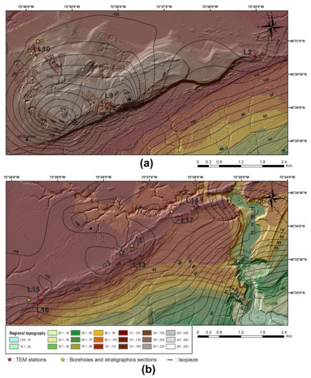
Figure 5.
(a) Interpolated water table elevation and regional piezometry of the eastern Saint-Narcisse moraine near Notre-Dame-du-Mont-Carmel in Mauricie, Quebec; (b) interpolated water table elevation and regional piezometry of the central Saint-Narcisse moraine near Ste-Geneviève-de-Batiscan and St-Narcisse in Mauricie, Quebec. The water table elevations are expressed in meters above sea level for both figures.
4.2. TEM Calibration
Figure 3 presents the induced voltage decay of Line 2, Station 3 (near YL071) and also represents the induced (and similar) voltage decay curves of Line 2, stations 1 and 2. Figure 4 (Section L2) illustrates the local surface deposit, the location of a stratigraphic cross-section (YL071) taken on the side of a sandpit, and the 2D section obtained on the basis of three TEM stations. The manually acquired piezometric surveys and piezometric map identify the water table at about 11 m depth. The electrical resistivity values associated with stratigraphic cross-section YL071 are 650–695 Ωm for unsaturated sand and gravel, 465–625 Ωm, and for unsaturated fine to medium sand (Table S1 in the Supplementary Materials).
Figure 6 (Section L3) shows a 2D section and a borehole stratigraphy (F1-PACES) recovered from an unsaturated subsoil. This TEM line comprises two stations. The induced voltage decay of Station 1, located near the borehole, shows a similar pattern as the induced voltage decay of Station 2 (Figure S1A in the Supplementary Materials). Here, the water table is not attained by the borehole, and a thick layer of clay is found at 12 to 46 m depth. The resistivity values for the stratigraphic units of the F1-PACES borehole are 350–405 Ωm for medium-to-coarse sand, 110–350 Ωm for fine to medium sand with silt and clay and 15–110 Ωm for clay in these unsaturated conditions (Table S1 in the Supplementary Materials). The presence of a small amount of silt and clay in fine to medium sand at 6 to 12 m depth decreases the electrical resistivity values considerably.
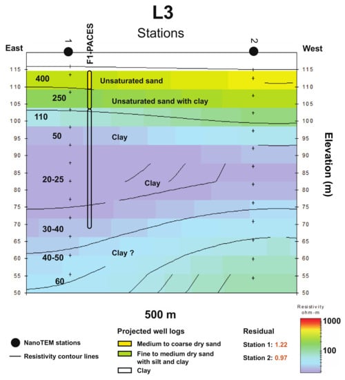
Figure 6.
Interpreted 2D Section L3 and borehole F1-PACES collected near Saint-Maurice, Quebec. The surface deposit elevation is obtained from lidar data. At the site, no groundwater was observed, and the basement was completely dry and mainly composed of clay.
Figure 7 (Section L7) presents a 2D section, and two stratigraphic sections (YL016 and YL018) collected on the side of a sandpit. These two sections are located at different elevations (129 and 134 m, respectively) and can be superimposed to create a composite (COMP016-18). This section was acquired on top of a sandpit with three TEM stations. The induced voltage decay of Station 1 (located near YL071) is similar to other stations on this 2D section (Figure S1B). The manually acquired piezometric surveys and the interpolated piezometric map (Figure 5) identify a water table at about 14 m depth. The electrical resistivity values for the stratigraphic units that make up the COMP016-18 section are 460–720 Ωm for coarse unsaturated sand and gravel with boulders, 345–460 Ωm for medium-to-coarse unsaturated sand, and 170–330 Ωm for fine to medium saturated sand (Table S1).
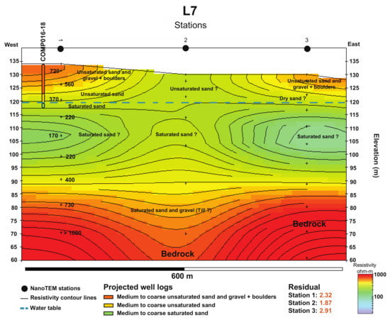
Figure 7.
Interpreted 2D Section L7 near Saint-Stanislas, Quebec. Stratigraphic cross-sections YL016 and YL018 have been Scheme 016. The surface deposit elevation is obtained from lidar data. The blue dashed line represents the projected water table from direct observations in the field. The legend indicates only the sediments observed in situ. The deeper sedimentary facies are deduced from the empirical and petrophysical relationship (i.e., the calibration chart).
Figure 8 (Section L10) reveals the local surface deposits of a 2D section with a borehole (MAUR0345) to the northwest and a stratigraphic cross-section (YL080) taken from the side of a sandpit to the southeast. This 2D section was obtained using six TEM stations. Figure S1C presents a typical induced voltage decay profile from the sector. For this 2D section, which is more than 350 m in length, the water table is located at a depth of 14 m (Figure 5) to the northwest and increases slightly, by a few meters, to the southeast. The electrical resistivity values for the stratigraphic units that make up the YL080 cross-section (fine and medium-to-coarse unsaturated sand) are 380–550 Ωm in unsaturated conditions (Table S1). The electrical resistivity values recorded for borehole MAUR0345 are 400–835 Ωm and 250–400 Ωm in unsaturated and saturated sand and gravel, respectively (Table S1).
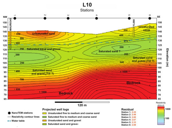
Figure 8.
Interpreted 2D Section L10, stratigraphic cross-section YL080, and borehole MAUR0345 acquired near Notre-Dame-du-Mont-Carmel, Quebec. The surface deposit elevation is obtained from lidar data. The 6 m variation of the water table height is probably due to a marked topographical variability of the bedrock surface as well as the regional topographic gradient, which increases rapidly toward the southeast.
Figure 9 (Section L13) presents a 2D section obtained for a saturated subsoil. The 2D section is derived from three TEM stations and two boreholes (ME0704; P12) recovered near the village of Saint-Narcisse. The manually acquired piezometric surveys and the interpolated piezometric map place the water table near the surface at less than 2 m depth. Figure S1D exhibits a typical induced voltage decay profile obtained for this sector. The resistivity values for the stratigraphic units that make up the ME0704 borehole are 150–230 Ωm for sand and gravel, 60–150 Ωm for sand and gravel with clay, and 40–60 Ωm for clay, all units in saturated conditions (Table S1). For the P12 drill site, the electrical resistivity values are 110–150 Ωm for saturated sand. West of the 2D Section L13, a 10 m-thick clay lens (at least) lies at a depth of about 20 m and reduces the electrical resistivity values considerably.
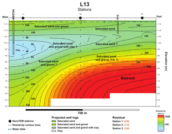
Figure 9.
Interpreted 2D Section L13 and borehole ME0704 acquired near Saint-Narcisse, Quebec. The surface deposit elevation is obtained from lidar data.
Finally, Figure 10 (Section L17) reveals the local surface deposit of a 2D section acquired from three TEM stations and the available borehole (ME0954), located on the northern side of the moraine near the village of Saint-Narcisse. The induced voltage decay of Station 1, which is located near the borehole, is similar to that of stations 2 and 3. The water table is located at 8 m depth to the west and gradually approaches the surface, reaching a depth of less than 1 m on the eastern side of the section. The electrical resistivity values for the stratigraphic units that make up the ME0954 borehole are 300–415 Ωm in unsaturated sand and gravel, 180–300 Ωm in saturated sand and gravel, 110–180 Ωm in saturated sand, and 60–110 Ωm in saturated sand with clay (Table S1). Table S1 also details other nearby TEM stations (L6_ST5; L6_ST7; L15_ST1) having stratigraphic cross-sections that were used to create the resistivity chart.
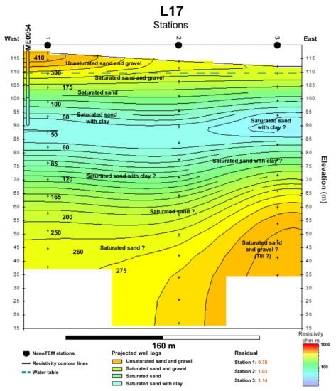
Figure 10.
Interpreted 2D Section L17 and borehole ME0954 acquired near Saint-Narcisse, Quebec. The surface deposit elevation is obtained from lidar data.
Since TEM profiles are interpolations between 1D soundings, the limitations of this approach bear uncertainty related to the interpolation and the smoothing. In fact, it is challenging to determine precisely which types of sediment are found at depth (and between the stations) only with indirect measurement (i.e., geophysics). However, within a distance of 22 km (east–west) in the St-Narcisse moraine in Mauricie, 13 TEM stations out of the 40 stations available in this zone can be compared to boreholes or stratigraphic cross-sections nearby. In addition, the piezometric map also provides additional information and allows us to validate the presence of saturated sediments, regardless of the shortcomings inherent to the inversion process (smoothing) and interpolation. Consequently, this significant amount of field data (boreholes, stratigraphic cross-sections, and 365 piezometric surveys) helps to decrease the uncertainty related to smoothing and interpolation between TEM stations and greatly strengthen the stratigraphic interpretation.
Here are the guidelines and some thresholds used to globally delimit the units: At depth (at the base of Figure 4, Figure 7, Figure 8, Figure 9 and Figure 11, Figures S3 and S4), when the resistivity values are greater than 900 Ωm, we estimate that the bedrock is reached. Between 500 and 900 Ωm, mainly tills (sand and gravel with pebbles/boulders) are overlying the bedrock, which is according to the literature [7,8,9]. On the surface, the resistivity values range between 400 and 850 Ωm, suggesting that there is a presence of unsaturated sand and gravel with pebbles/boulders or unsaturated sand. When the water table is reached, the resistivity decreases sharply along the entire length of the TEM sections, indicating saturated sediments. If the values range between 100 and 400 Ωm, it suggests saturated sand and gravel or saturated sand. In order to determine the sediment classes with the greatest possible accuracy, we also based our observations on the continuity of the surface layers that we observed during the fieldwork, but mainly on stratigraphic cross-sections and boreholes available near the TEM sections. We hypothesized that if the resistivity values are relatively constant with depth, the type of sediment will stay similar. For example, if unsaturated sand is observed at the surface, and the resistivity values are relatively stable below the water table, the unsaturated sand is probably perpetuated at depth. When changes in resistivity are less gradual and more abrupt, there appears to be a change in sediment class that can be linked to a variation of porosity (and then a variation of water content) and so probably to heterogeneity. Alternatively, the low resistivity values can also be linked to a higher clay content within granular sediment. If the resistivity values are lower than 110, we mainly find clay or mixed clay.
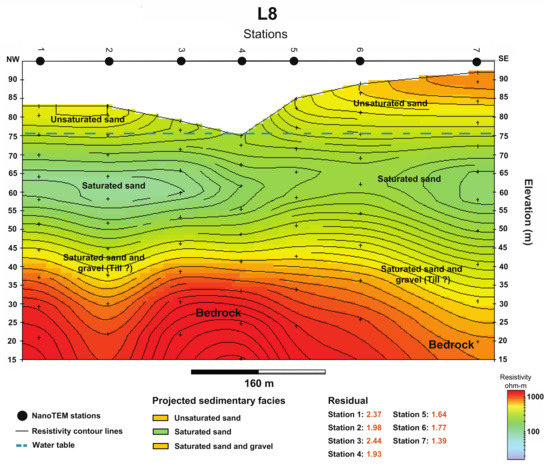
Figure 11.
Interpreted 2D Section L8 near Saint-Narcisse and Saint-Geneviève-de-Batiscan, Quebec. The surface deposit elevation is obtained from lidar data.
4.3. Compilation and Calibration Chart
Table 1 and Figure 11 lists the electrical resistivity values obtained for each type of unsaturated and saturated Quaternary sediment found in the Saint-Narcisse moraine. Seven sediment classes are represented in the calibration chart: (1) unsaturated sand, (2) saturated sand, (3) unsaturated sand and gravel with pebbles/boulders, (4) saturated sand and gravel, (5) unsaturated sand, sand, and gravel (all with clay), (6) saturated sand, sand and gravel (all with clay), and (7) clay. When the sediments are saturated with water or contain clay, resistivity values are low and generally less than 400 Ωm; clay sediments produce the overall lowest values and reach a maximum resistivity of 110 Ωm. Resistivity values for clay usually vary between 15 and 110 Ωm (Table S1; Figure 11). As the proportion of sand and gravel to clay increases, so does resistivity. For the unsaturated sand with clay, the resistivity varies with a correspondingly low resistivity, ranging between 110 and 350 Ωm (unsaturated) and 60 and 360 Ωm (saturated). In comparison, unsaturated and saturated sands have a resistivity range of 345–650 Ωm and 110–330 Ωm, respectively (Figure 11). The potential increase in resistivity from saturated to unsaturated sand can reach up to 88% at maximum values (345–650 Ωm). Unsaturated and saturated sand and gravel with pebbles/boulders produce respective resistivity ranges of 370–835 Ωm and 150–400 Ωm (Figure 11). The potential increase from saturated to unsaturated sand and gravel can reach up to 109% (400–835 Ωm).

Table 1.
Measured electrical resistivity of Quaternary sediments in the Saint-Narcisse moraine, eastern Mauricie, Quebec, Canada.
4.4. TEM Results
4.4.1. Western Sector (Notre-Dame-du-Mont-Carmel)
Figure 1 shows the location of three 2D TEM sections in the western portion of the study area (Figure 4 and Figure 8, Figure S3). From the produced calibration chart, Figure 8 (2D Section L10) shows saturated sand and saturated sand and gravel at a depth of 10 to 15 m. The thickness of this water-saturated zone varies between 25 and 35 m and extends over a length of approximately 350 m. A layer of saturated sand and gravel overlies the bedrock in this area. Further southeast, about 2.5 km from Section L10, the 2D Section L9 (Figure S3) also shows the presence of saturated sand at about 15 m depth. This layer of saturated sand varies between 30 and 50 m thick and extends more than 1 km from east to west. The observations from borehole ME1843 and the calibration chart show that the sediments found in L9 are, from top to bottom, sand and gravel interspersed with fine to medium sandy facies and then sand and gravel, pebbles, and boulders overlying the bedrock. From the stratigraphic section YL071 and the calibration chart (Figure 4), Section L2, situated 3 km northeast of Section L9, also shows the presence of saturated sand (as observed for sections L9 and L10) at about 10 to 15 m depth, which juxtaposes a layer of saturated sand and gravel overlying the bedrock. In Section L2, the thickness of the saturated granular sediments varies between 35 and 45 m and extends (east–west) over a distance of 75 m.
4.4.2. Central Sector (Saint-Narcisse)
Six 2D TEM sections (Figure 9, Figure 10, Figure 11, Figures S4, and S6A,B; sections L13, L17, L8, L14, L15, and L16) lie within the central zone of the moraine, situated southeast of the village of Saint-Narcisse and west of the Batiscan River (Figure 1 and Figure 2). The four stations of the 2D Section L16 (Figure S6B) attain a depth of about 76 m without reaching bedrock. The produced calibration chart (Table 1) indicates the presence of saturated granular sediment from the top to the bottom of Section L16, containing (1) fine to coarse saturated sand (western side) and saturated sand and gravel (eastern side); (2) saturated sand with clay; and (3) saturated sand or saturated sand and gravel. The saturated sediment in L16 has a lateral east–west extension of 200 m (length of Section L16) and a thickness varying between 66 and 76 m. The subsurface layers exposed in Section L16 appear very similar to those of the 2D Section L15 (Figure S6A), located approximately 300 m to the north (Figure 1). Section L15 comprises three stations, and the calibration chart indicates the presence of >87 m thick, saturated sand over a distance of at least 200 m (east–west). The main difference relative to Section L16 is that the resistivity values in Section L15 increase at about 35 m depth. This increase suggests the presence of saturated sand and gravel between 35 and 80 m depth. At 2.5 km northeast of sections L15 and L16 lies the 2D Section L13 (Figure 9), which comprises three stations. Similar to sections L15 and L16, Section L13 also shows the presence of saturated sediment. Boreholes ME0704 and P12 and the calibration chart indicate that the Section L13 sediments are, from top to bottom, saturated sand (east) and saturated sand and gravel (west) at the surface. On the western side of Section L13, between 15 and 35 m depth, a clay lens drags down the resistivity values to 40 Ωm. Around the clay lens on the eastern side of Section L13, the resistivity is higher, and the borehole ME0704 shows the presence of sand and gravel mixed with clay. The higher resistivity values at the base of Section L13 (Figure 9) are associated with saturated sand and gravel, pebbles, and boulders. Here, the saturated granular sediment (i.e., sand, sand, and gravel) varies in thickness from 25 to 70 m with an extension (east–west) over nearly 1 km. The variations in bedrock topography for Section L13 generate a larger range in the aquifer thickness. The 2D cross-sections of sections L17 and L14 (Figure 10 and Figure S4) are located about 1.5 km northeast of Section L13 in the north-central part of the moraine. Sections L17 and L14 comprise four and three stations, respectively, with respective lengths of 500 m and 200 m. Borehole ME0954 and the calibration chart indicate that these two sections are composed of sand and gravel with variable amounts of clay and sandy facies at depth, 50 to 80 m depth for Section L17 and 42 to 75 m depth for Section L14. These two sections contain saturated granular sediments (from top to bottom: sand and gravel with clay, sand with clay, sand, sand, and gravel) with a thickness varying between 31 and 94 m. The thickness of the sediments depends mainly on the topographic undulations of the bedrock. The two combined lines indicate saturated sediment extending over nearly 700 m along an east–west axis. Finally, the 2D Section L8 (Figure 11) is located 2.5 km south of sections L14 and L17. Section L8 comprises seven stations, totaling 600 m in a north–south axis. According to the calibration chart, this section shows the bedrock overlain by sand and gravel and sandy facies (saturated and unsaturated). The saturated sediment varies in thickness from 25 to 35 m and extends over 600 m (i.e., the full length of Section L8). In the central sector of the moraine, these six 2D sections (L8, L13, L14, L15, L16, and L17) have a total length of 2.5 km and cover an area of approximately 21 km2 (Figure 1 and Figure 11). Typical induced voltage decay profiles (1D smooth inversion model) obtained for each section are available in the Supplementary Materials (Figures S1D, S2A–D, and S5A,B).
5. Discussion
5.1. Sedimentary Facies Resistivity
Variation in electrical resistivity relates to the electrical resistivity of water being much lower than that of soils [50,51,52], and resistivity is much lower for sediments having a high water content [16,53]. The circulation of the electric current in the basement, however, takes place mainly by volume conduction (or electrolytic conduction) through the pore water of these formations [50,53]. Thus, the conduction of an electric current occurs primarily through the water contained in the pores or at the interface between the minerals and the pore water (surface electrical conductivity).
The calibrated chart highlights that electrical resistivity values for unsaturated sand and sand and gravel with pebbles/boulders are much higher, potentially up to 97% higher than for these same sediments when saturated. Clay has a low resistance to the passage of an electric current, and the resistivity values are low to very low. If clay horizons are found within sand or sand and gravel facies, the resistivity can decrease to 60 Ωm (Table 1). Low resistivity is a function of surface conduction from the higher clay mineral concentrations (Reynolds 2011). In contrast, sand/gravel/pebbles are much less conductive and provide greater resistance to the passage of an electric current. Grain size and even grain shape can also alter the bulk electrical and dielectric behaviors, thus affecting resistivity values [16,54].
The greater resistivity associated with increased grain size is visible, for example, at the base of several 2D sections of the Saint-Narcisse moraine (sections L2, L7, L8, L9, L10, L13, L14, and L17). During deglaciation, juxtaglacial and fluvioglacial deposits (e.g., ice-marginal outwash) generated by the melting ice were superimposed onto the glacial till sequence left by the passage of the LIS [7,9]. Fine-grained sediments (e.g., clay and silt) have high conductivity and low resistance to the passage of electric currents; resistivity increases as sediment grain size coarsens. The calibration chart reflects these particle size changes; therefore, the chart links the sedimentary facies (i.e., clay, sand, sand, and gravel), the associated electrical resistivity, and water content. Although overlap exists in the distributions between sediment classes and making the interpretation quite difficult, some of the resistivity ranges are well separated (Figure 12). In particular, saturated and unsaturated sediment shows very little overlap for the same category of sediment (i.e., saturated and unsaturated sand; saturated and unsaturated sand and gravel; Figure 12), which means that TEM is able to accurately identify the presence of water, except when there is a significant amount of clay mixed with the granular sediment, which drags down the resistivity. It is also challenging to discriminate between sand and gravel and the sand due to their close range of resistivity. Although these two categories show substantial overlap (Figure 12) and illustrate an inherent lack of the chart, the main objective of this study is to determine the presence of water (saturated sediment) with the greatest possible precision in order to identify potential aquifers. Consequently, even if these two sediment classes share similar resistivity values, they have a common characteristic, which is to be lithological units of high permeability that can be crossed by water and possibly act as a reservoir. In fact, the presence of saturated and unsaturated granular sediments (i.e., below and above the water table), regardless of their granulometric size, can be validated with relative precision by the piezometric contour map (Figure 5), the boreholes, and the stratigraphic cross-sections. Indeed, even if there is an overlap between these categories of sediments and the TEM profiles are interpolations between 1D soundings and bears uncertainty related to these interpolations, the direct data (i.e., piezometric map built with 465 piezometric surveys, the boreholes, and the stratigraphic cross-sections) strengthen the stratigraphic interpretation and thus reduce the erroneous hypotheses linked to smoothing, interpolations and overlaps. Moreover, the ultimate goal of this study is essential to identify the presence of underground water and its spatial continuity.
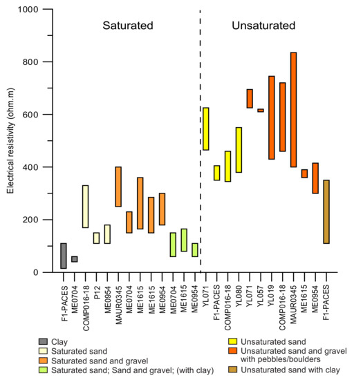
Figure 12.
Respective resistivity for the seven sediment classes proposed in the calibration chart. They are deduced from borehole logs to display the minimum and maximum values for each saturated and unsaturated sediment. The horizontal axis represents each of the boreholes and stratigraphic cross-sections and their associated facies. The bedrock is not considered in this figure.
5.2. Relationship between the Calibration Chart and the TEM Sections
Geophysical data provide an effective alternative to borehole surveys for characterizing the internal structures of deposits. The extrapolation of geophysical results over the entire study area requires creating a calibration chart to relate obtained electrical resistivity values to various unsaturated and saturated sediments. Once the calibration is achieved, however, multiple TEM profiles can be obtained in a short time span, and the stratigraphy of a large area can be evaluated. An equivalent characterization using boreholes is often impractical given the time-consuming and expensive nature of borehole drilling campaigns. Furthermore, cores are generally limited in number with considerable spacing between sites, making correlations between boreholes difficult.
The developed electrical resistivity chart (Table 1) allows us to use all collected 2D TEM sections west of the Batiscan River. Several 2D sections (Figure 13, Figures S3 and S6A,B; sections L8, L9, L15, and L16) cannot be associated with any stratigraphic cross-sections, boreholes, or piezometric surveys, but nonetheless, provide valuable information regarding the geometry and extension of groundwater tables at the regional scale. These TEM sections, which can be linked to the other TEM sections used to build the calibration chart (Figure 4, Figure 8, Figure 9, Figure 10 and Figure S4; sections L2, L10, L13, L17, and L14), therefore provide additional stratigraphic information and permit the assessment of a much larger zone of the Saint-Narcisse moraine. The linking of sedimentology and geophysical data provides much insight in regard to the scale, arrangement, and granulometry of the sediment facies and their associated hydrogeological properties. The geophysical results of our study can support hydrogeological inferences of aquifer thickness, variation, and continuity.
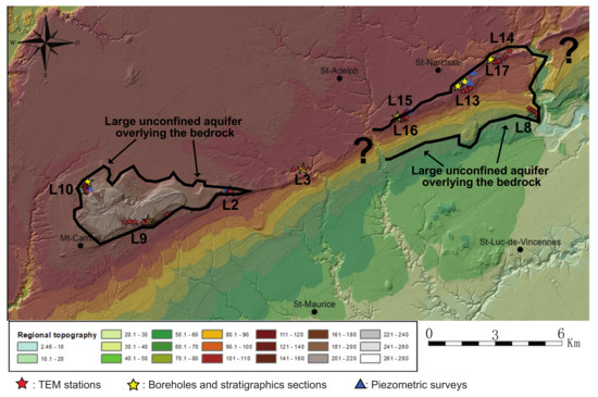
Figure 13.
Regional topography of the study area and location of TEM stations, boreholes, stratigraphic cross-sections, and piezometric surveys acquired on the Saint-Narcisse moraine, Quebec. The black lines delimit two large unconfined regional aquifers west of Notre-Dame-du-Mont-Carmel and southeast of Saint-Narcisse.
5.3. Hydrogeological Exploration Targets
5.3.1. Western Sector (Notre-Dame-du-Mont-Carmel)
Three 2D TEM sections (sections L2, L9, and L10) have a total length of 1.4 km and are spread over an area of approximately 11 km2 east of Notre-Dame du Mont Carmel (Figure 13). These TEM sections share a similar sediment architecture and several other geological similarities; thus, we can assume a stratigraphic continuity and a hydraulic connection between these sections. For these three sections, we observed that (1) the bedrock is located between 45 and 65 m for each of the 14 TEM stations; (2) a few meters of glacial till (i.e., sand and gravel) overlie the bedrock; (3) 5 to 15 m of unsaturated granular sediments, mainly sand/sand and gravel, are deposited over the surface of the moraine; (4) small amounts of clay are intermixed with the granular sediment. Greater amounts of clay would provide a natural impermeable barrier and increase the heterogeneity of the environment, thereby reducing the hydraulic connections at local and regional scales; and (5) the thickness of the water-saturated granular sediment varies between 30 and 60 m, the changes in sediment thickness being related to variations in local bedrock topography.
Previous studies have demonstrated that the sector of the moraine near Notre-Dame-du-Mont-Carmel (Figure 1) is composed primarily of granular sediments overlying bedrock, a continuity of the stratigraphic units, and the presence of extensive unconfined regional aquifers [7,11,35,55]. These Quaternary sequences consist of subglacial or melt-out till (i.e., mainly sand and gravel) deposited during the last glaciation and the Saint-Narcisse readvance, proximal and distal glaciomarine deposits (mainly fine, medium, and coarse sands lay down by the Champlain Sea), as well as juxtaglacial and fluvioglacial deposits [7,9]. The saturated sediment and the water table elevation (Figure 5) also suggest a continuity of stratigraphic units and a hydraulic connection in this sector of the moraine. When we compare the piezometric contour of Figure 5 with the decrease in resistivity values associated with saturated sediments for each TEM section, the depth generally correlates within 1 to 3 m. The drop in resistivity values is caused by the transition from unsaturated to saturated sediment at the top of the groundwater table. This strong correlation combined with a low RMS (i.e., 2.96 m), associated with a high-quality model, suggests that the piezometric map is representative of reality and that a hydraulic connection does exist between the TEM lines (i.e., sections L2, L9, and L10) in the sector of Notre-Dame-du-Mont-Carmel. In this case, the piezometric contours reflect the continuity of the water table elevation as well as the saturated sediments between the TEM sections. By correlating sections L2, L9, and L10 and assuming that the areas where no geophysical data have been collected have such continuity for their stratigraphic units, we can deduce, as Légaré-Couture et al. (2018) hypothesized previously, that an unconfined aquifer covers the entire area northeast of Notre-Dame-du-Mont-Carmel (Figure 13). This large aquifer has a lateral extension of more than 6 km, a thickness varying from 30 to 60 m, and a depth between 5 and 15 m from the surface.
5.3.2. Central Sector (Saint-Narcisse)
These six 2D TEM sections of this part of the morainic complex (i.e., sections L8, L13, L14, L15, L16, and L17) have a total length of 2.7 km and are spread over an area of approximately 19.5 km2 southeast of the village of Saint-Narcisse (Figure 13). Except for Section L8, few unsaturated sediments are recorded within these TEM sections, and the water table is near the surface, generally varying between 1 and 5 m depth. The bedrock is much deeper here than around the Notre-Dame-du-Mont-Carmel area, sometimes even up to 94 m (sections L15, L16, and L17) below the surface. This observation also agrees with previous studies, which sometimes locate the bedrock under the moraine as much as 100 m below present sea level [11]. This regional configuration (a deep bedrock and a shallow water level) and the substantial thicknesses of granular sediment deposits (i.e., sand, sand and gravel, sand and gravel with clay) into a series of bedrock depressions observed along the Saint-Narcisse moraine are suitable for creating unconfined aquifers. Moreover, according to previous studies, the thickest deposits can reach 150 m in south Mauricie [11]. The water-saturated sediments in the central section of the moraine are therefore quite thick, varying from 30 to over 94 m in thickness. The low amount of clay intermixed with the granular sediment observed in the TEM sections of this area of the moraine also suggests a suitable hydraulic connection owing to the absence of impermeable barriers at the local and regional scales. The Quaternary sequences and the type of sediment deposited within the central section of Saint-Narcisse moraine are similar to those within the Notre-Dame-du-Mont-Carmel area (i.e., subglacial or melt-out till, proximal and distal glaciomarine deposits, juxtaglacial and fluvioglacial deposits). In addition, the piezometric contour of Figure 5 is also well correlated with the decreased resistivity associated with saturated sediments for each of the TEM sections. This drop in resistivity is caused by the transition from unsaturated to saturated sediment at the top of the groundwater table. In the Notre-Dame-du-Mont-Carmel sector, the strong correlation between the piezometric contour and the TEM sections, as well as a low RMS, also suggests that the produced piezometric map is representative of the actual regional stratigraphy and sediments. Consequently, a hydraulic connection owing to the continuity of the stratigraphic units does exist between the TEM sections in this area of the moraine located southeast of the village of Saint-Narcisse. Here, the piezometric contour reflects the continuity of the water table elevation and the saturated sediments between the TEM sections. Finally, by correlating these six TEM sections (i.e., sections L8, L13, L14, L15, L16, and L17) and assuming that the areas characterized by an absence of collected geophysical data show a continuity of their stratigraphic units, it is possible to identify a vast unconfined aquifer in the central sector of the moraine (Figure 13). From these assumptions, this aquifer covers an area of more than 6.5 × 3.0 km (>19.5 km2), varies between 25 and more than 94 m thick (depending on the sector), and is usually found within 1 to 2 m of the surface of the moraine.
5.3.3. Compartmentalization of the Aquifers
The Saint-Narcisse moraine in the Mauricie region contains thick layers of well-sorted sand and gravel deposits and holds two large unconfined aquifers overlying the bedrock. According to Légaré et al. (2018), although the hydrostratigraphy of the moraine is complex, it nonetheless contains a large regional unconfined aquifer within the surface sands. The Saint-Narcisse moraine has hydrogeological conditions favorable for groundwater extraction, and most municipalities located along the moraine and on the adjacent marine clay plain (e.g., Saint-Narcisse, Saint-Prosper, Saint-Maurice, Notre-Dame-du-Mont-Carmel, and Sainte-Geneviève-de-Batiscan) already draw their drinking water from this aquifer [11], which attests to the aquifer capacity of these sectors. Previous studies have hypothesized the presence of these large regional aquifers on the basis of the large quantity of granular sediments at the moraine’s surface [11,46,56].
Our study validates the presence of these aquifers (Figure 13) and goes further by providing precise information related to regional stratigraphy and the aquifers’ geometry, thickness, and extension. This study also suggests compartmentalization of the aquifers and a discontinuity of the stratigraphic units within the Saint-Narcisse moraine in the area. This compartmentalization separates the aquifers from each other and is mainly produced by the presence of less permeable sediments, as the discontinuous nature of the moraine is frequently interrupted by multiple sections composed of finer sediments deposited by the Champlain Sea [6]. Both granular aquifers (Figure 13), from the surface, do not appear to be connected hydraulically because of the presence of these low-permeability barriers (e.g., mud units; Figure 6) that limit groundwater flow between this pair of highly conductive bodies [7,11,35,55,56].
6. Conclusions
The TEM method used in this study of the Saint-Narcisse moraine in the Mauricie region of Quebec revealed the compartmentalization of a multi-kilometer morainic system. Mud units deposited by the Champlain Sea during the deglacial marine incursion act as impermeable barriers to create a discontinuity of the stratigraphic granular units within the moraine and the compartmentalization of its contained aquifers. TEM demonstrated its utility for investigating the stratigraphic nature and the production of initial hydrogeological maps of other remote territories and geological contexts that lack minimal stratigraphic and piezometric information. To use all TEM results acquired for this study, we built an electrical resistivity calibration chart for saturated and unsaturated Quaternary sediments applying specifically to the St-Narcisse moraine in eastern Mauricie. The procedure can also be used in various environments if there are enough data. This chart links granulometric facies (i.e., clay, sand, sand, and gravel) and their respective electrical resistivity and water content. Once calibrated and applied to several TEM profiles along the Saint-Narcisse moraine, the chart helped identify two large unconfined granular aquifers overlying the bedrock west of the Batiscan River. Within the study area, these aquifers extend for a minimum distance of 12 km (east–west) and vary in thickness between 25 and more than 94 m. The TEM approach offers a relatively fast, simple, inexpensive, non-destructive, and effective means of acquiring valuable groundwater-related information to help municipalities and local entrepreneurs manage regional groundwater and ensure its preservation. Our findings highlight the need for more detailed studies of the Saint-Narcisse morainic complex to better assess its groundwater resources. Greater details regarding this pair of identified aquifers can be obtained using direct approaches, including pumping tests, boreholes, and a more detailed hydrogeological mapping of targeted areas.
Supplementary Materials
The following are available online at https://www.mdpi.com/article/10.3390/geosciences11100415/s1, Table S1. TEM stations, with all nearby boreholes and stratigraphic sections, and their associated electrical resistivity values. Depths are identified by parentheses. The blue color in the electrical resistivity column represents the approximate depths at which the water table has been reached. The water table has been determined by (1) in situ observations and (2) use of the piezometric map; Figure S1. A. Left: Typical induced voltage decay from Line 3 (L3), Station 1. Measured data are shown as crosses and inversion fitting as a black line. Noise level is approximately 10 μV/A. The inversion residual is 1.22. B. Left: Typical induced voltage decay from Line 7 (L7), Station 1. Measured data are shown as crosses and inversion fitting as a black line. Noise level is approximately 10 μV/A. The inversion residual is 2.32. C. Left: Typical induced voltage decay from Line 10 (L10), Station 1. Measured data are shown as crosses and inversion fitting as a black line. Noise level is approximately 10 μV/A. The inversion residual is 2.35. D. Left: Typical induced voltage decay from Line 13 (L13), Station 1. Measured data are shown as crosses and inversion fitting as a black line. Noise level is approximately 25 μV/A. The inversion residual is 0.82. Right for Figure S1A–D: The obtained smooth model TEM inversion; Figure S2. A. Left: Typical induced voltage decay from Line 17 (L17), Station 1. Measured data are shown as crosses and inversion fitting as a black line. Noise level is approximately 8 μV/A. The inversion residual is 0.78. B. Left: Typical induced voltage decay from Line 9 (L9), Station 1. Measured data are shown as crosses and inversion fitting as a black line. Noise level is approximately 30 μV/A. The inversion residual is 1.66. C. Left: Typical induced voltage decay from Line 8 (L8), Station 5. Measured data are shown as crosses and inversion fitting as a black line. Noise level is approximately 9 μV/A. The inversion residual is 1.64. D. Left: Typical induced voltage decay from Line 14 (L14), Station 2. Measured data are shown as crosses and inversion fitting as a black line. Noise level is approximately 10 μV/A. The inversion residual is 0.78. Right for Figure S2A–D: The obtained smooth model TEM inversion; Figure S3. Interpreted 2D Section L9 and borehole ME1843 near Notre-Dame-du-Mont-Carmel, Quebec. The surface deposit elevation is obtained from lidar data. The blue dashed line represents the projected water table, and all direct observations have been acquired in the field; Figure S4. Interpreted 2D Section L14 near Saint-Narcisse, Quebec. The surface deposit elevation is obtained from lidar data; Figure S5. A. Left: Typical induced voltage decay from Line 15 (L15), Station 1. Measured data are shown as crosses and inversion fitting as a black line. Noise level is approximately 30 μV/A. The inversion residual is 0.95. B. Left: Typical induced voltage decay from Line 16 (L16), Station 3. Measured data are shown as crosses and inversion fitting as a black line. Noise level is approximately 15 μV/A. The inversion residual is 0.49. Right for Figure S5A,B: The obtained smooth model TEM inversion; Figure S6. A. Interpreted 2D Section L15 near Saint-Narcisse, Quebec. B. Interpreted 2D Section L16 near Saint-Narcisse, located approximately 300 m further south of L15. The surface deposit elevation of both sections was obtained from lidar data.
Author Contributions
Y.L. performed the measurements, analyzed the data, interpretation and wrote the paper with input from all authors; J.W. and R.C. contributed to the writing, supervision, funding acquisition, and interpretation. All authors have read and agreed to the published version of the manuscript.
Funding
This research was funded by the Groundwater Knowledge Acquisition Program (PACES) and by the Natural Sciences and Engineering Research Council of Canada (NSERC) through a research postsecondary grant to Y.L., grant number ESD3-546526-2020.
Institutional Review Board Statement
Not applicable.
Informed Consent Statement
Not applicable.
Data Availability Statement
PACES LME data is not yet published, but it will be published in a database of the Government of Quebec, Canada. So for now, we exclude this statement because the study did not report any data.
Acknowledgments
We thank the PACES team for allowing us to collect the necessary geophysical data in summer 2020. We also sincerely thank Anouck Ferroud (PACES-UQAC) for her help collecting the core F1-PACES in autumn 2019, as well as Mélanie Lambert (PACES-UQAC) and David Noel (UQAC) for their technical support and advice during the collecting and processing of data and for explaining the operation of many of the geophysical instruments.
Conflicts of Interest
The authors declare no conflict of interest.
References
- Parriaux, A.; Nicoud, G. De la montagne à la mer, les formations glaciaires et l’eau souterraine. Exemple du contexte Nord-alpin occidental. Quaternaire 1993, 4, 61–67. [Google Scholar] [CrossRef]
- Burt, A.K. Three-dimensional hydrostratigraphy of the Orangeville Moraine area, southwestern Ontario, Canada. Can. J. Earth Sci. 2018, 55, 802–828. [Google Scholar] [CrossRef]
- Sass, O. Determination of the internal structure of alpine talus deposits using different geophysical methods (Lechtaler Alps, Austria). Geomorphology 2006, 80, 45–58. [Google Scholar] [CrossRef]
- McClymont, A.F.; Hayashi, M.; Bentley, L.R.; Muir, D.; Ernst, E. Groundwater flow and storage within an alpine meadow-talus complex. Hydrol. Earth Syst. Sci. 2010, 14, 859–872. [Google Scholar] [CrossRef]
- Schrott, L.; Hufschmidt, G.; Hankammer, M.; Hoffmann, T.; Dikau, R. Spatial distribution of sediment storage types and quantification of valley fill deposits in an alpine basin, Reintal, Bavarian Alps, Germany. Geomorphology 2003, 55, 45–63. [Google Scholar] [CrossRef]
- Daigneault, R.-A.; Occhietti, S. Les moraines du massif Algonquin, Ontario, au début du Dryas récent, et corrélation avec la Moraine de Saint-Narcisse. Géographie Phys. Quat. 2006, 60, 103–118. [Google Scholar] [CrossRef][Green Version]
- Occhietti, S. The Saint-Narcisse morainic complex and early Younger Dryas events on the southeastern margin of the Laurentide Ice Sheet. Géographie Phys. Quat. 2007, 61, 89–117. [Google Scholar] [CrossRef]
- Occhietti, S.; Chartier, H.M.; Hillaire-Marcel, C.; Cournoyer, M.; Cumbaa, S.L.; Harington, R. Paléoenvironnements de la mer de Champlain dans la région de Québec, entre 11 300 et 9750 bp: Le site de Saint-Nicolas. Géographie Phys. Quat. 2001, 55, 23–46. [Google Scholar] [CrossRef]
- Occhietti, S. Stratigraphie du Wisconsinien de la région de Trois-Rivières-Shawinigan, Québec. Géographie Phys. Quat. 1977, 31, 307–322. [Google Scholar] [CrossRef]
- Girard, F. Architecture et Hydrostratigraphie d’un Complexe Morainique et Deltaïque dans la Région de Saint-Raymond de Portneuf, Québec. Ph.D. Thesis, Université du Québec, Institut National de la Recherche Scientifique, Quebec, QC, Canada, 2001. [Google Scholar]
- Légaré-Couture, G.; Leblanc, Y.; Parent, M.; Lacasse, K.; Campeau, S. Three-dimensional hydrostratigraphical modelling of the regional aquifer system of the St. Maurice Delta Complex (St. Lawrence Lowlands, Canada). Can. Water Resour. J./Rev. Can. Ressour. Hydr. 2017, 43, 92–112. [Google Scholar] [CrossRef]
- Palacky, G. Resistivity characteristics of geological targets. In Electromagnetic Methods in Applied Geophysics; Nabighian, M., Ed.; Society of Exploration Geophysicists: Tulsa, OK, USA, 1987; pp. 55–129. [Google Scholar]
- Palacky, G. Use of airborne electromagnetic methods for resource mapping. Adv. Space Res. 1993, 13, 5–14. [Google Scholar] [CrossRef]
- Sørensen, K.I.; Auken, E.; Thomsen, P. TDEM in Groundwater Mapping–A Continuous Approach. In Proceedings of the Symposium on the Application of Geophysics to Engineering and Environmental Problems 2000, Arlington, VA, USA, 20–24 February 2000. [Google Scholar]
- Danielsen, J.E.; Auken, E.; Jørgensen, F.; Søndergaard, V.; Sørensen, K.I. The application of the transient electromagnetic method in hydrogeophysical surveys. J. Appl. Geophys. 2003, 53, 181–198. [Google Scholar] [CrossRef]
- Reynolds, J.M. An Introduction to Applied and Environmental Geophysics, 2nd ed.; John Wiley & Sons: Hoboken, NJ, USA, 2011; ISBN 1119957141. [Google Scholar]
- Goldman, M.; Kafri, U. Geoelectric, Geoelectromagnetic and Combined Geophysical Methods in Groundwater Exploration in Israel. In The Many Facets of Israel’s Hydrogeology; Springer: Berlin/Heidelberg, Germany, 2020; pp. 299–393. [Google Scholar]
- Larocque, M.; Meyzonnat, G.; Ouellet, M.-A.; Graveline, M.-H.; Gagné, S.; Barnetche, D.; Dorner, S. Projet de Connaissance des Eaux Souterraines de la Zone Vaudreuil-Soulanges. Rapport Synthese; Université du Québec à Montréal: Montréal, QC, Canada, 2015. [Google Scholar]
- Chesnaux, R.; Lambert, M.; Walter, J.; Fillastre, U.; Hay, M.; Rouleau, A.; Daigneault, R.; Moisan, A.; Germaneau, D. Building a geodatabase for mapping hydrogeological features and 3D modeling of groundwater systems: Application to the Saguenay–Lac-St.-Jean region, Canada. Comput. Geosci. 2011, 37, 1870–1882. [Google Scholar] [CrossRef]
- Walter, J.; Rouleau, A.; Chesnaux, R.; Lambert, M.; Daigneault, R. Characterization of general and singular features of major aquifer systems in the Saguenay-Lac-Saint-Jean region. Can. Water Resour. J./Rev. Can. Ressour. Hydr. 2017, 43, 75–91. [Google Scholar] [CrossRef]
- Douglas, R.J.W.; Poole, W.H.; Sanford, B.V.; Williams, H.; Kelly, D.G. Geology and Economic minerals of Canada. In Geology and Economic Minerals of Canada; Geological Survey of Canada: Ottawa, ON, Canada, 1970; Volume 1, pp. 649–662. [Google Scholar]
- Globensky, Y. Géologie des Basses-Terres du Saint-Laurent; Ministère de L’énergie et des Ressources: Québec, QC, Canada, 1987. [Google Scholar]
- Rivers, T.; Van Gool, J.; Connelly, J.N. Contrasting tectonic styles in the northern Grenville province: Implications for the dynamics of orogenic fronts. Geology 1993, 21, 1127–1130. [Google Scholar] [CrossRef]
- Nadeau, L.; Brouillette, P. Carte structurale de la région de Shawinigan (SNRC 31I), Province de Grenville, Québec. Comm. Géologique Canada Doss. Public 1995. [Google Scholar] [CrossRef]
- Parent, M.; Occhietti, S. Late Wisconsinan deglaciation and glacial lake development in the Appalachians of southeastern Québec. Géographie Phys. Quat. 1999, 53, 117–135. [Google Scholar] [CrossRef]
- Parent, M.; Occhietti, S. Late Wisconsinan Deglaciation and Champlain Sea Invasion in the St. Lawrence Valley, Québec. Géographie Phys. Quat. 1988, 42, 215–246. [Google Scholar] [CrossRef]
- Dyke, A.S.; Prest, V.K. Late Wisconsinan and Holocene History of the Laurentide Ice Sheet*. Géographie Phys. Quat. 1987, 41, 237–263. [Google Scholar] [CrossRef]
- Dietrich, J.; Bunya, S.; Westerink, J.J.; Ebersole, B.A.; Smith, J.M.; Atkinson, J.H.; Jensen, R.; Resio, D.T.; Luettich, R.A.; Dawson, C.; et al. A High-Resolution Coupled Riverine Flow, Tide, Wind, Wind Wave, and Storm Surge Model for Southern Louisiana and Mississippi. Part II: Synoptic Description and Analysis of Hurricanes Katrina and Rita. Mon. Weather. Rev. 2010, 138, 378–404. [Google Scholar] [CrossRef]
- Margold, M.; Stokes, C.; Clark, C.D. Ice streams in the Laurentide Ice Sheet: Identification, characteristics and comparison to modern ice sheets. Earth-Sci. Rev. 2015, 143, 117–146. [Google Scholar] [CrossRef]
- Stokes, C. Deglaciation of the Laurentide Ice Sheet from the Last Glacial Maximum. Geogr. Res. Lett. 2017, 43, 377. [Google Scholar] [CrossRef]
- Lévesque, Y.; St-Onge, G.; Lajeunesse, P.; Desiage, P.; Brouard, E. Defining the maximum extent of the Laurentide Ice Sheet in Home Bay (eastern Arctic Canada) during the Last Glacial episode. Boreas 2019, 49, 52–70. [Google Scholar] [CrossRef]
- Benn, D.; Evans, D.J.A. Glaciers and Glaciation, 1st ed.; Routledge: London, UK; New York, NY, USA, 2014; ISBN 1444128396. [Google Scholar]
- Evans, D. Glacial Landsystems, 1st ed.; Routledge: London, UK; New York, NY, USA, 2014; ISBN 1444119168. [Google Scholar]
- Landry, B.; Beaulieu, J.; Gauthier, M.; Lucotte, M.; Moingt, S.; Occhietti, S.; Pinti, D.L.; Quirion, M. Notions de Géologie, 4th ed.; Modulo: Montréal, QC, Canada, 2012; ISBN 2-89113-256-4. [Google Scholar]
- Tricart, J.; Occhietti, S. Le Quaternaire de la région de Trois-Rivières-Shawinigan, Québec. Contribution à la paléogéographie de la vallée moyenne du St-Laurent et corrélations stratigraphiques. In Annales de Géographie; Armand Colin: Paris, France, 1983; Volume 92, pp. 242–245. [Google Scholar]
- Nabighian, M.N. Electromagnetic Methods in Applied Geophysics; Society of Exploration Geophysicists: Tulsa, OK, USA, 1991; Volume 2. [Google Scholar]
- Fitterman, D.V.; Labson, V.F. Electromagnetic Induction Methods for Environmental Problems. In Near-Surface Geophysiscs; Society of Exploration Geophysicists: Tulsa, OK, USA, 2005; pp. 301–356. [Google Scholar]
- Fitterman, D.V.; Stewart, M.T. Transient electromagnetic sounding for groundwater. Geophysics 1986, 51, 995–1005. [Google Scholar] [CrossRef]
- Parsekian, A.; Singha, K.; Minsley, B.; Holbrook, W.S.; Slater, L. Multiscale geophysical imaging of the critical zone. Rev. Geophys. 2014, 53, 1–26. [Google Scholar] [CrossRef]
- Kafri, U.; Goldman, M.; Lang, B. Detection of subsurface brines, freshwater bodies and the interface configuration in-between by the time domain electromagnetic method in the Dead Sea Rift, Israel. Environ. Earth Sci. 1997, 31, 42–49. [Google Scholar] [CrossRef]
- Kalisperi, D.; Kouli, M.; Vallianatos, F.; Soupios, P.; Kershaw, S.; Lydakis-Simantiris, N. A Transient ElectroMagnetic (TEM) Method Survey in North-Central Coast of Crete, Greece: Evidence of Seawater Intrusion. Geosciences 2018, 8, 107. [Google Scholar] [CrossRef]
- MacInnes, S.; Raymond, M. Zonge Data Processing Two-Dimensional, Smooth-Model CSAMT Inversion version 3.00; Zonge Engineering and Research Organization, Inc.: Edwardstown, Australia, 2001; p. 41. [Google Scholar]
- MacInnes, S.; Raymond, M. STEMINV: Smooth Model TEM Inversion. Zo. Eng. Tucson, AZ. 2005. Available online: http://zonge.com/instruments-home/software/modeling-tem/ (accessed on 17 August 2021).
- Constable, S.; Parker, R.L.; Constable, C. Occam’s inversion: A practical algorithm for generating smooth models from electromagnetic sounding data. Geophysics 1987, 52, 289–300. [Google Scholar] [CrossRef]
- Dewar, N.; Knight, R. Estimation of the top of the saturated zone from airborne electromagnetic data. Geophysics 2020, 85, EN63–EN76. [Google Scholar] [CrossRef]
- McCormack, R. Etude hydrogéologique de la rive nord du Saint-Laurent. In Énergie et Ressource Naturelle; Service des Eaux Souterraines: Québec, QC, Canada, 1983; Volume 15, p. 188. ISBN 2550029399. [Google Scholar]
- Zimmerman, D.; Pavlik, C.; Ruggles, A.; Armstrong, M. An Experimental Comparison of Ordinary and Universal Kriging and Inverse Distance Weighting. Math. Geol. 1999, 31, 375–390. [Google Scholar] [CrossRef]
- Jones, N.L.; Davis, R.J.; Sabbah, W. A comparison of three-dimensional interpolation techniques for plume characterization. Ground Water 2003, 41, 411–419. [Google Scholar] [CrossRef]
- Wise, S. Assessing the quality for hydrological applications of digital elevation models derived from contours. Hydrol. Process. 2000, 14, 1909–1929. [Google Scholar] [CrossRef]
- Abu-Hassanein, Z.S.; Benson, C.H.; Blotz, L.R. Electrical Resistivity of Compacted Clays. J. Geotech. Eng. 1996, 122, 397–406. [Google Scholar] [CrossRef]
- Shukla, S.K.; Yin, J.-H. Fundamentals of Geosynthetic Engineering, 1st ed.; Taylor and Francis, Balkema: London, UK, 2006; ISBN 1482288443. [Google Scholar]
- Pandey, L.M.; Shukla, S.K.; Habibi, D. Electrical resistivity of sandy soil. Geotech. Lett. 2015, 5, 178–185. [Google Scholar] [CrossRef]
- McCarter, W.J. The electrical resistivity characteristics of compacted clays. Geotechnique 1984, 34, 263–267. [Google Scholar] [CrossRef]
- Kemna, A.; Binley, A.; Slater, L. Crosshole IP imaging for engineering and environmental applications. Geophysics 2004, 69, 97–107. [Google Scholar] [CrossRef]
- Ferland, P.; Occhietti, S. Révision du stratotype des Sédiments de Saint-Pierre et implications stratigraphiques, vallée du Saint-Laurent, Québec. Géographie Phys. Quat. 1990, 44, 147–158. [Google Scholar] [CrossRef][Green Version]
- Grenier, C.; Denis, R. Etude hydrogeomorphologique dans la region du Lac Maskinongé, Québec. Can. J. Earth Sci. 1974, 11, 733–754. [Google Scholar] [CrossRef]


Publisher’s Note: MDPI stays neutral with regard to jurisdictional claims in published maps and institutional affiliations. |
© 2021 by the authors. Licensee MDPI, Basel, Switzerland. This article is an open access article distributed under the terms and conditions of the Creative Commons Attribution (CC BY) license (https://creativecommons.org/licenses/by/4.0/).