Article

Are Past Sea-Ice Reconstructions Based on Planktonic Foraminifera Realistic? Study of the Last 50 ka as a Test to Validate Reconstructed Paleohydrography Derived from Transfer Functions Applied to Their Fossil Assemblages

EPOC (Environnements & Paléoenvironnements Océaniques et Continentaux) Laboratory, UMR 5805, Bordeaux University, Allée Geoffroy Saint Hilaire, 33615 Pessac, France
*
Author to whom correspondence should be addressed.
Geosciences 2021, 11(10), 409; https://doi.org/10.3390/geosciences11100409
Submission received: 31 July 2021 / Revised: 21 September 2021 / Accepted: 24 September 2021 / Published: 28 September 2021
(This article belongs to the Special Issue Application of Foraminifera in Biochronology)

Abstract

:
Since its existence, paleoceanography has relied on fossilized populations of planktonic foraminifera. Except for some extreme environments, this calcareous protist group composes most of the silty-to-sandy fraction of the marine sediments, i.e., the foraminiferal oozes, and its extraction is probably the simplest among the currently existing set of marine fossil proxies. This tool has provided significant insights in the building of knowledge on past climates based on marine archives, especially with the quantification of past hydrographical variables, which have been a turning point for major comprehensive studies and a step towards the essential junction of modelling and paleodata. In this article, using the modern analog technique and a database compiling modern analogs (n = 1007), we test the reliability of this proxy in reconstructing paleohydrographical data other than the classical sea-surface temperatures, taking advantage of an update regarding a set of extractions from the World Ocean Atlas for transfer functions. Our study focuses on the last glacial period and its high climatic variability, using a set of cores distributed along the European margin, from temperate to subpolar sites. We discuss the significance of the reconstructed parameters regarding abrupt and extreme climate events, such as the well-known Heinrich events. We tested the robustness of the newly obtained paleodata by comparing them with older published reconstructions, especially those based on the complementary dinoflagellate cyst proxy. This study shows that the potential of planktonic foraminifera permits going further in reconstructions, with a good degree of confidence; however, this implies considering ecological forcings in a more holistic perspective, with the corollary to integrate the message of this fossil protist group, i.e., the obtained parameters, in light of a cohort of other data. This article constitutes a first step in this direction.

1. Introduction

Planktonic foraminifera (PF) have constituted key material for paleoceanographers, especially for stratigraphical and hydrographical reconstructions, for nearly a century (e.g., from Phleger, 1939 [1] to Schiebel et al., 2018 [2]; CLIMAP [3]). Their shells are at the basis of nearly all the biochronological scales established for marine sequences during the Quaternary. They provide not only valuable raw material for stratigraphical determinations (especially radiocarbon dating and stable-isotope measurement), but also and above all diverse and well-preserved fossil assemblages, which are at the basis of paleoenvironmental reconstructions (e.g., from Pflaumann et al., 1996 [4] to Siccha and Kučera, 2017 [5] and references therein). However, as calcareous proxies, their robustness is also known to be limited in some extreme conditions, especially in oceanographical basins where either the lysocline or the temperature of the first hundred-meter-water column hamper their preservation or diversity (e.g., Kučera et al., 2005 [6,7]; Nguyen and Speijer, 2019 [8]; Greco et al., 2019 [9] and 2021 [10]).
Recently, in parallel with an effort to diversify the PF tool, its modern calibration and accuracy were reconsidered and challenged [9,11,12]. Apart from geochemical considerations on their tests, major questions were raised regarding the value of fossil assemblages in deciphering basin-wide hydrological past changes, since complex patterns of habitats (depending on seasonality and water depth, for instance) are known for PF populations. For example, working on the basis of high-latitude assemblages is often hampered by their monospecific diversity, with the polar species Neogloboquadrina pachyderma nearly exclusively dominating the assemblages. However, weaknesses can also be strengths, as, conversely, monospecific polar assemblages are outstanding markers of specific cold events within glaciations (e.g., Ruddiman, 1977 [13]; Eynaud et al., 2009 [14]).
In this context, approaches relying on the compilation of modern eco-biogeographical databases derived from the analysis of recently fossilized populations in the topmost oceanic sediment layers provide comprehensive sets which have considerably improved our bioclimatic knowledge of PF. These modern sedimentary spectra, analyzed for their contents/relative abundances in PF, offer the advantage of integrating regional taphonomic processes; furthermore, they can be statistically tested and exploited to provide proxies of oceanic conditions, as conducted, for instance, with transfer functions sensu lato ([6,12]; Guiot and de Vernal, 2007 [15]).
Here, we test the robustness of the modern analog technique to reconstruct past hydrography with PF assemblages, focusing on the North Atlantic Ocean (Figure 1), using (1) a training set of modern analogs (n = 1007), improved with new extractions of oceanic parameters from the World Ocean Atlas (initiated with de Vernal et al., 2020 [16]), and (2) calculations based on key archives covering the last 50 thousand years. We document the coherency of the results obtained for past hydrographical changes regarding the climatological context of this period; further, we focus on the parameters directly or indirectly quantifying the sea-ice cover evolution at millennial scales in comparison with other tools, providing comparable reconstructions. The investigations here conducted are especially fruitful and rich of learnings for Heinrich events (HEs), which punctuate the last 50 ka. They also question the robustness of PF assemblages in providing accurate paleohydrographical contexts, despite the recurrent criticisms on the accuracy of this historical fossil tool.

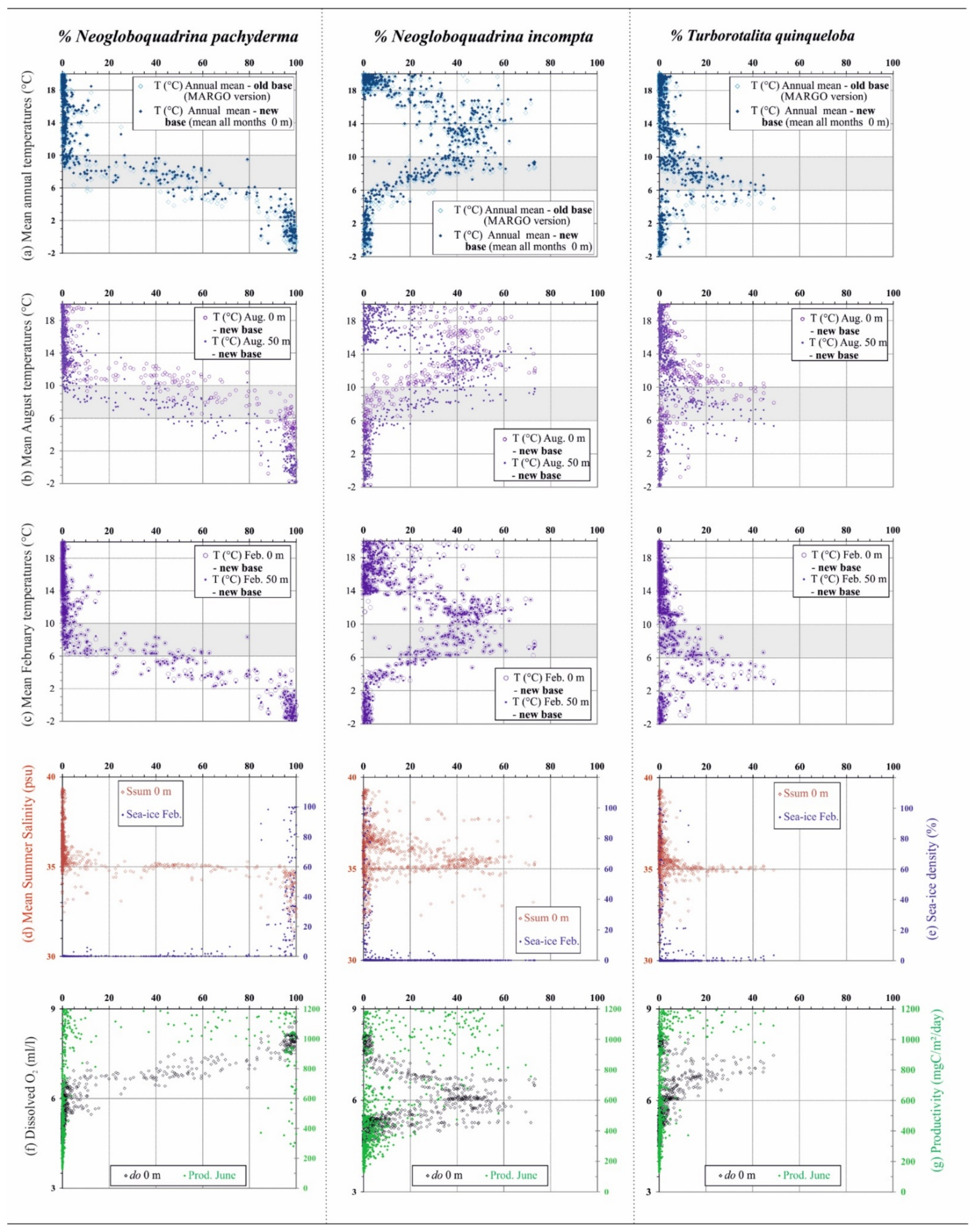
2. Past Hydrographical Quantifications Based on Planktonic Foraminifera

Prior to its application in the present study, the methodology used to quantify past hydrography, i.e., the Modern Analog Technique (MAT), has been tested several times on different reference marine records (see [17,18,19,20,21] for concrete produced data and [22,23] for a review on this approach), using the MAT1007 transfer function developed at EPOC, based on the MARGO program (multiproxy approach for the reconstruction of the glacial ocean surface [6,7,24,25]). The performed calculations rely on a statistical comparison among past assemblages and a modern reference database of 1007 modern samples distributed in the North Atlantic Ocean and its adjacent seas, including the Nordic seas (Figure 1a). Using a script developed by Guiot and Brewer (https://www.eccorev.fr/spip.php?article389, accessed on 25 August 2021) for the R software (“R” version 2.7.0, R Development Core Team, 2008), the statistical assessment of the distance between the fossil and modern assemblages was obtained. Hydrographical parameters were thus estimated from an average weighted inversely to the distance (or dissimilarity) of the five best analogues selected. The significant novelty, here introduced, is that the set of parameters reconstructed on the basis of PF was considerably enlarged thanks to an update of the modern hydrographical references. Usually, published reconstructions based on PF assemblages are limited to sea-surface temperatures (SSTs). This limitation is the result of long lasting questionings on the significance of the derived reconstructions with regard to the ecology of PF. It is difficult to disentangle ecological parameters in the marine realm [25] and SSTs often carry the most significant weight in the distribution of species [12]. However, following what has been obtained with other fossil protist groups, we decided to go beyond this limitation in order to expand the potential of the PF tool.
The new hydrographical set was generated mostly thanks to extractions obtained from the World Ocean Atlas 2013 (WOA13; https://www.nodc.noaa.gov/OC5/woa13/woa13data.html, accessed on 20 September 2018). These data permit reconstructing quantified past SSTs and salinities at two depths, i.e., 0 and 50 m, to infer thermocline migration for means calculated monthly, seasonally (according to the astronomical definition of seasons [26]), or annually. In this study, we performed calculations for the whole set of new parameters; however, here, we only report annual, winter (i.e., January–February–March) and summer (i.e., July–August–September) means, together with seasonal extremes (i.e., the warmest, August, and the coldest, February, month of the year). The derived errors (root mean square error of prediction (RMSEP)) calculated for each reconstructed parameter were a maximum of 1.4 °C, for temperatures, and of 0.7 psu, for salinities (in August, at 0 m); these maximal error values are plotted on graphs hereafter. Reconstructions of sea-surface dissolved oxygen (do), phosphate and nitrate concentrations were also obtained thanks to our new WOA13 extractions, but only do is here presented (with an RMSEP of 0.1 mL/L on past reconstructions). Their significance as key ecological parameters of the North hemisphere marine planktonic fossil populations was tested with the updated dinocyst transfer function published in 2020 (see [16] for details, especially for multivariate analysis). Sea-ice cover (SIC) data, compiled at a ¼-degree resolution from the NSIDC website (http://nsidc.org/data/G10010, 20 September 2021, see [16]), are now also updated in the database. They are expressed in two ways and conform strictly to the extractions conducted for dinocysts [16] in order to provide comparable past quantified reconstructions; SIC data are expressed as SIC mean monthly concentrations (coverage percentages from 0 to 100%; in this article, only February means are shown, with an RMSEP of 10%) and SIC duration (number of months/year with sea-ice concentration >50%, with an RMSEP of 1.5 month/year).
Monthly primary productivity (PP) values (obtained from NASA’s Moderate Resolution Imaging Spectroradiometer (MODIS) database; https://modis.gsfc.nasa.gov/data/dataprod, 20 September 2021, see [16] for the extraction methodology) were also introduced for PF for the same purpose, i.e., to test their relevance and potential versus the dinocyst tool for common reconstructions, particularly in relation to the same cores in the North Atlantic. In this article, only PP values for June are shown (with an RMSEP of 360 mgC/m3/day).
Regarding PF assemblages, the modern spectra constituting the dataset (with no change since the compilation of the database based on the MARGO program) were also tested using statistical tools and graphic mappings, focusing on the biogeography of the species (see Figure 2 for species response curves and also references [14,23]). The modern biogeography of PF is fairly well known at the scale of oceanic basins (ever since the study by Bé and Tolderlund, 1971 [27]) and has even been numerically modeled ([28,29] and references therein), despite some outstanding uncertainties regarding the parameters describing their habitats; for instance, the depths at which PF can live have not yet been well defined. Using the topmost sediment deposits as a modern reference for their biogeography somewhat circumvents this limitation, as the deposited and fossilized assemblages are the result of a temporal integration over several years, as well as the result of a three-dimensional spatial integration. This type of integration was also applied to the requests performed for modern parameters, as they were extracted over a time window of several decades (1955–2012), with a spatial resolution grid of one degree at maximum (with a minimum size of a 1/12 degree spatial resolution for PP, see [16]); this spatial resolution is key for the description of the scale of oceanic structures (e.g., [30]).
The graphs plotted in Figure 2 are enough to show how modern PF populations, even if tracked, here, with the sedimentological filter, are sensitive to hydrographical parameters. The fairly narrow SST ranges of distribution for PF clearly illustrate specific restricted habitats (and a high degree of endemicity) for the selected species, with, interestingly, the SST interval of 6–10 °C identifying a key physical barrier for those species, regardless of the season. These values are typical of the ones registered in the modern subpolar latitudinal bands. The tolerance for salinity variations is greater for Neogloboquadrina incompta, whose distribution is known to be more ubiquitous in the North Atlantic than Neogloboquadrina pachyderma (NP) and Turborotalita quinqueloba. Further, this species seems to be distributed along a wide range of PP contexts (with low dissolved oxygen contents), whereas the two most polar species only occur in high abundance for high PP values (over 800 mgC/m2/day) and well oxygenated surface-waters.
As shown in Figure 2, the newly extracted oceanic parameters provide the opportunity to test the significance of a more complete set of ecological variables, especially among those known to impact PF distribution and/or those that have been critical during extreme past climatic changes, i.e., the thermocline position versus the depth of the mixed layer (compare, for instance, Figure 2b,c, where the temperatures at 0 m and 50 m depths are plotted), both known here thanks to the new information related to the temperature at 50 m, but also thanks to the dissolved oxygen content, which is also correlated to productivity conditions. Among the parameters to be tested in order to determine past conditions, those related to the SIC are crucial for a better understanding of the oceanic changes associated to melt-water events, such as those linked to HEs or stadials.
To validate the robustness of the calculations regarding past periods, reconstructions derived from the study of four marine cores (mapped in Figure 1), which were already published on the basis of the MAT transfer function (Table 1), were run for this new set of oceanic data. This set of cores embraces a modern SST range of 8 °C along the western European margin (from warm temperate (40° N) to subpolar environments (63° N)). We also tested the coherency of the reconstructions with other proxies; the newly produced quantified data were then compared to existing ones derived from other bioindicators (dinocysts especially) when possible. The age models of the compiled sequences were not modified, and they all conform to the last ones published (see references in Table 1).

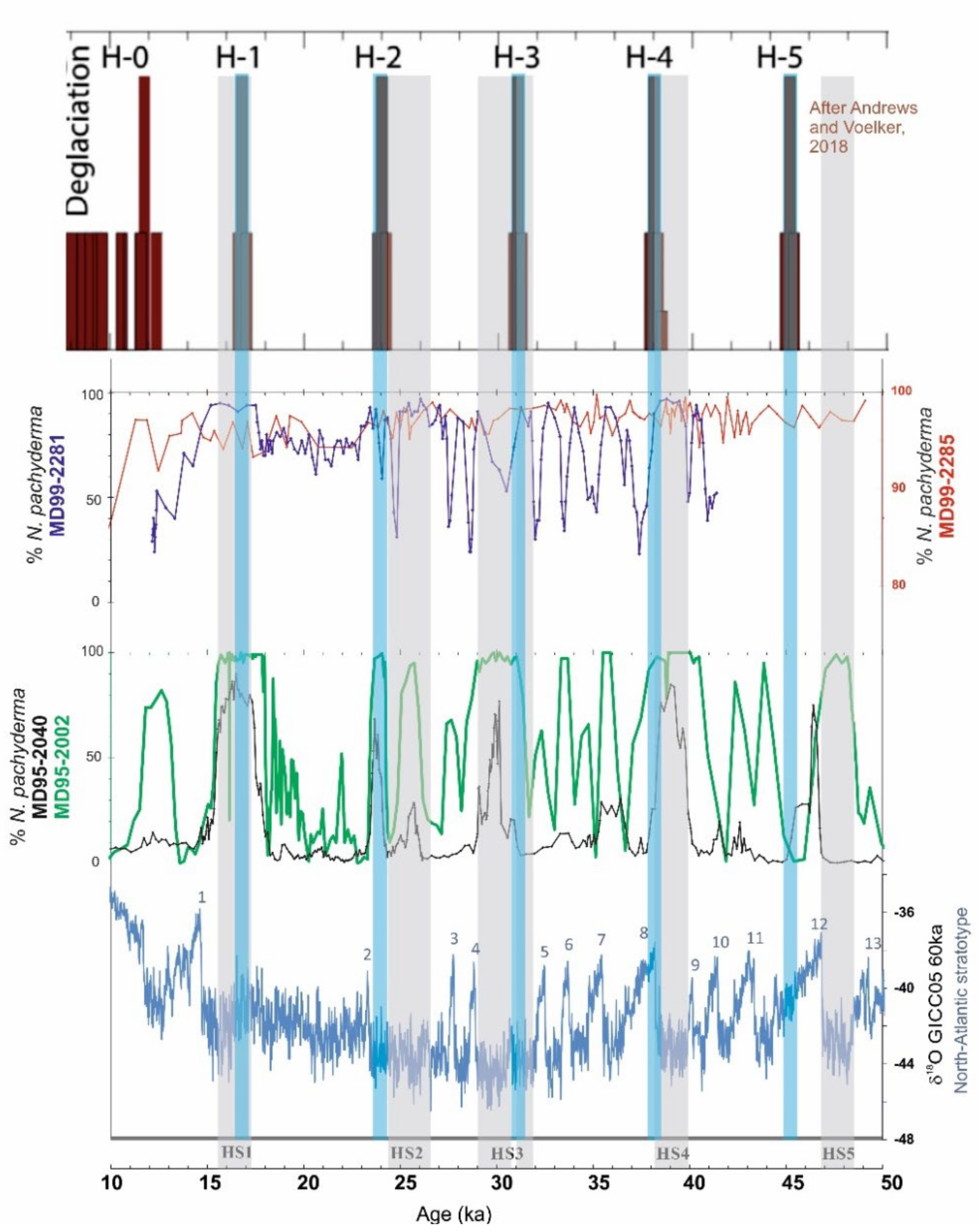
3. Heinrich Events and Their PF-Derived Signatures

3.1. Basic Features and Knowledge

The recent comprehensive work on HEs by Andrews and Voelker (2018) [45] has drawn a capital, timely constrained and defined framework for the distribution of those climatic and ecological dramatic disruptions (Figure 3). Their review pertinently reaffirmed and underlined that HEs are complex, multiphase events and demonstrated that their causalities and effects have often been amalgamated.
HEs are specific to glacial periods, the most recent six being called HEs sensu stricto (Heinrich et al., 1988 [49]; excluding the Younger Dryas event, despite this event being called H0 on the North Atlantic western side [50]). HE-like events have also been recognized during penultimate glaciations up to one million years BP (e.g., [51,52]); some cold periods within interglacial stages have been assimilated to occur in oceanic conditions similar to those of HEs, with a disruption of the Atlantic Overturning circulation ([53,54,55] and references therein). During the last glaciation, they were part of contrasting climatic extremes in relation to the well-known stadial and interstadial pacing of Dansgaard Oeschger (DO) cycles (Dansgaard et al., 1993 [56,57]; see Figure 3). Their impacts on the marine realm were vast [58,59,60,61] and they are known to be marked by drastic sea-surface population changes in the North Atlantic; those changes are commonly used as biostratigraphical tie intervals, especially based on PF assemblages (from [13] to [48]).
Thus, the 50–10 ka interval constitutes a key time period for testing our reconstructions and their reliability, both for determining the chronological pacing of the detected events and for validating the recorded hydrographical shifts. To achieve this, we selected four cores from different locations along the western European margin (Figure 1, Table 1) in order to capture a sensitivity gradient based on the new extractions and MAT calculations. The selected cores were all used in key articles which have contributed to enlarge our knowledge on the marine counterpart expression of HEs/DO and can be considered as reference records for the western European margin (see references in Table 1).
The relevance of their selection is expressed in Figure 3, where the simple use of the abundance of the polar species NP, as a basic bioindicator of the last 50 ka of climatic history, underlines marked shifts in PF populations. Those shifts were detected along the entire latitudinal gradient covered by the chosen set of cores. A poleward decrease in their amplitudes, mirrored by steady NP abundances during cold events (including HEs and stadials) and warmings, was recorded. As expected, the PF sensitivity was saturated in the polar domains, where NP occurs in monospecific values. This problem was raised very soon with PF reconstructions as a severe hamper to their use with no precaution in cold environments to track past hydrographical changes (e.g., [4,7]). It is also worth noting the time lag recorded latitudinally during the deglacial warming after HE1. Finally, the “ideal” sensitivity window to track hydrographic changes with PF seems to be the temperate belt, as seen with the MD95-2002 NP record.

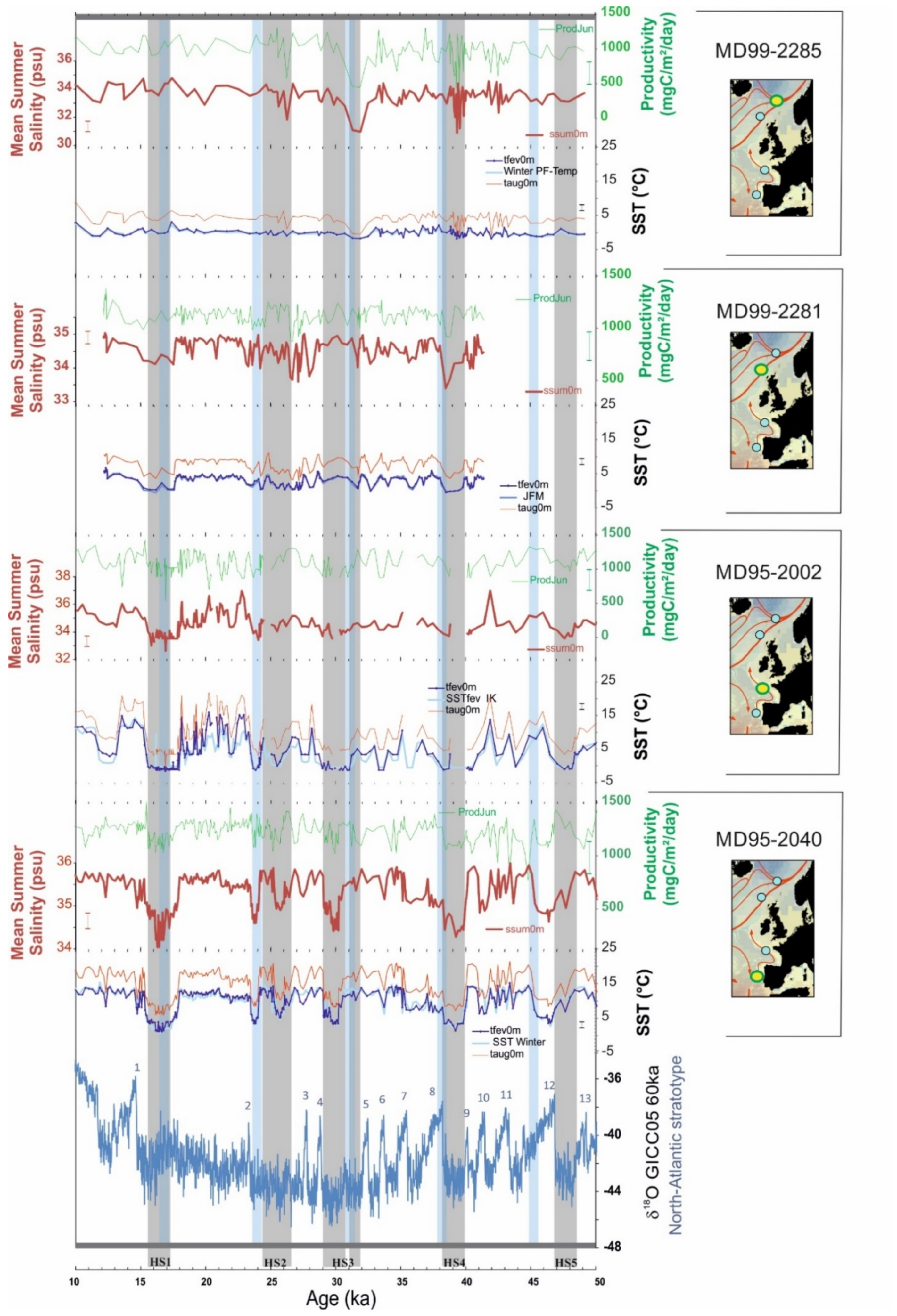
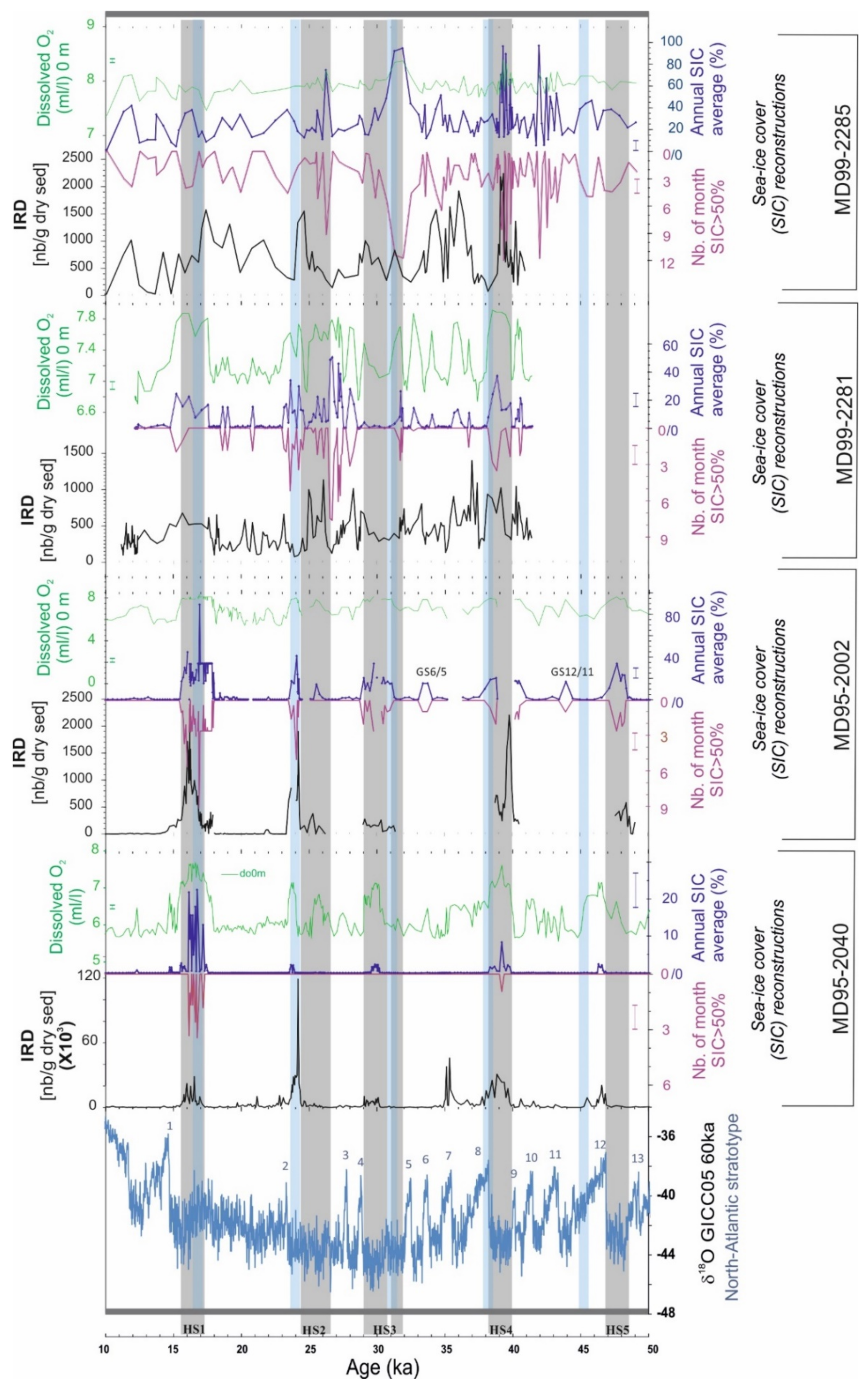
3.2. New Hydrographic Signals to Better Understand HEs

In this article, we focus on the study of specific newly reconstructed parameters which bring relevant constraints on sea-surface conditions during HEs, such as salinities, SIC, oxygenation and productivity. The objective is to test their significance in relation to existing knowledge about HE-induced changes in the North Atlantic Ocean. At this stage, the absolute values reconstructed thanks to the new database cannot be considered exact, as more tests are needed to infer the ecological patterns which relate PF populations to the newly extracted parameters, especially regarding correlations and inter-regulation among the different parameters. The fundamental laws at the basis of PF-based transfer function development indicate that, as with most of the marine species, PF distribution is accurately predicted exclusively by SSTs. Thus, SSTs have long been traditionally and routinely reconstructed with a high degree of confidence in Paleoceanography on the basis of PF assemblages. Yet, how ecological parameters relate to each other is a key question in the marine realm and no true independency exists in this environment characterized by the absence of perennial physical barriers. Consequently, our procedure was to first consider the SST results, as their reproducibility is a way to infer the strength of the method, irrespectively the implements accompanying any update of the database. This important validation step is illustrated in Figure 4, in which are compiled, for each of the selected cores, in the range 50–10 ka, the reconstructed SSTs at 0 m for August and February; for the latter, the plot of the most recent published data based on PF transfer functions is shown in the same graph, using the same scale (however, data are not always from the same database or the same method of calculations; see Table 1). This comparison shows that the reproducibility is optimal, despite minor methodological discrepancies, arguing for a very robust mathematical approach. The summer means of the reconstructed salinities (this season being, for the boreal hemisphere, the one subject to the largest melting events) and productivities in June, are also plotted in Figure 4. Here, the latitudinal reduction in the sensitivity of PF can be again observed, as shown by the flattening of the signals obtained when approaching subpolar latitudes (note that salinities and PP are not displayed with identical scales for each core). The compilation drawn in Figure 4 shows that the reconstructed parameters closely correspond the reference climate variability known for the last glaciation; HEs, stadials and interstadials are imprinted in the reconstructed signals. This underlines the potential of PF populations in tracking climate changes and the desirable performance of transfer functions (here, MAT) sensu lato in converting variations in species/assemblages into quantified hydrographical values (other than SSTs). Decreases of up to 10 °C in SSTs (similar for winter and summer means) were recorded along the Iberian margin and in the Bay of Biscay during HEs (HE1 and HE4 having recorded the largest amplitude shifts). Higher salinities corresponded to higher temperatures and vice versa, with low values always being recorded during HEs. Salinity drops by a minimum of 2 units can be seen in all records; these values are coherent with previously reconstructed ones along the European margin [22,62]. Interestingly, the reconstructed productivity values do not follow the same trends as SST and salinity ones do (which can be superposed with a few deviant excursions); this suggests that the parameter of productivity is independent from the other two and that it probably finds expression in groups of species that are different from the ones that are firstly regulated by SSTs. Such finding stands as an incentive for pursuing efforts towards the diversification of parameters to reconstruct on the basis of PF. If, as already mentioned, using the absolute values for PP is unrealistic at this stage, we can nonetheless remark that coherent low values are reached during HEs, in agreement with previous studies [60,61]. Once again, this is very encouraging for further investigations focusing on the PF significance in productivity changes.
Figure 5 compiles original new reconstructions with a focus on indicators marking ice presence or dynamics in the past surface of the North Atlantic Ocean. Ice-rafted debris (IRD; i.e., large grains >150 µm) concentrations in the sediment obtained from previous publications (see Table 1; note that HE5 is not correctly dated in core MD95-2040, assigning a younger age to the IRD peak [32], which identifies its occurrence at this latitude) are here compared to the newly reconstructed do values and to SIC data (for concentration and duration, see Methods in Section 2). It is worth noting that reconstructed concentrations seem to point to a more sensitive response of PF, as additional events are identified using this parameter. The do values closely match DO climatic shifts, with cold events being systematically associated with higher oxygen contents, independent of the latitude. This could signify, as previously identified, low PP; however, it could also be due to a more dynamic surface ocean caused by iceberg drifting, together with the southward migration of major oceanic and climatic fronts.
In accordance with what is known of HEs, the maximum impact regarding (sea)-ice dynamics is recorded close to the sources of iceberg release (e.g., [13]). SIC variations are increasingly significant (reconstructed values largely above the RMSEP) and frequent when moving northwards. The subpolar basins of the North Atlantic Ocean recorded multiple events, in comparison to the Ocean temperate edge, where only extreme events are marked by the reconstructed parameters linked to ice occurrence. In fact, at 40° N, a SIC signal was recorded, but the reconstructed values are within the error bar of the reconstructions. The very discrete peaks identified at this latitude are strictly limited to HEs, but, interestingly, indices of ice presence derived from PF reconstructions and IRD deposits are not perfectly synchronous, except for HE1. Relative to the Iberian margin, the question about the hydrographical impact of icebergs during HEs remains unanswered; many authors believe that, if iceberg drifting occurred, their size and/or melting were not consequent enough to generate changes other than SST and salinity drops (e.g., [31,32,62,63]). The low values of the newly reconstructed SIC concentrations obtained with our approach do not permit to confirm whether sea-ice did, even episodically, develop during HEs, but its occurrence at this latitude merits to be questioned in future research.
There are no doubts on SIC developments during HEs when examining the northern Bay of Biscay, where durations of up to 3 months per year were recurrently recorded over the last 50 ka. Given this temperate record, HEs still appear as the most favorable circumscribed periods for SIC developments, although SIC occurrence is also seen for a limited number of stadials (two stadials between DO 12/11 and DO 6/5). The MD95-2002 record shows a complex structure of SIC developments within HEs, with no HE responding in the same way as the previous or following one. The largest SIC values were registered during moderate IRD peaks, with the largest recorded IRD amounts resulting in non-analogous situations within the newly tested database and, thus, in a lack of quantification. This result could be related to what was also detected in the two cores located further north. Though the SIC signal was less easily readable, as noise was introduced by shifts of similar amplitudes for HEs and stadials, here, again, the maximum SICs are not associated with maximum IRD releases. This is especially obvious for HE3 and HE2, with a larger SIC rather surrounding the core of HEs, where IRD pulses occurred. Such a situation is coherent with what is observed in the modern fjords of Greenland [64]; icebergs, even if calving from upstream glaciers, do not break out, as long as they are trapped in multiyear sea-ice (called sikussac by Dowdeswell et al., 2000 [64]), and their drifting, with IRD deposits, only occurs when the SIC is melting. This process was also simulated in the Weddell sea [65]. This can explain the apparent lack of synchronicity between IRD and SIC found in our results. Additionally, highly unsteady conditions, marked by a rupture of the thermocline and upwelling phenomena, also accompany large iceberg drifting [66,67], which may prevent SIC occurrence. Conversely, iceberg melting, by injecting freshwaters, may positively influence the formation of SIC [68]. Consequently, a direct relation between their presence and SIC is difficult to infer and requires the consideration of their latitudinal trajectories. During HEs, iceberg melting was predominant in the temperate belt (in what has been called the Ruddiman band [13,58]), but many complex feedbacks are associated with their surges and are far from being understood especially during the last glaciation [57]. This also includes considerations about the impact of iceberg melting on PP; if the low reconstructed values for this parameter, on the basis of our approach, are coherent with those in previous studies, this result shall be put in perspective with the recent work by Romero et al., 2021 [69], who assert that the melting of icebergs during past iceberg discharges along the Alaskan coasts contributed to the fertilization of the surface ocean layer.
As previously mentioned, oxygenation of surface water can bring some indices regarding the stability of the water column. The presence of do within the topmost layers of the ocean is a function of several main parameters, such as the ventilation of the water masses, itself a function of their degree of mixing and of the efficiency of their exchanges with the atmosphere (notably depending on SSTs), and, directly and indirectly, of PP. These parameters are highly variable in terms of latitudinal and geographical position (distance from the coast and, especially, from continental distributaries [70]). According to our reconstructions, PP was mostly low during HEs and do was high. This result itself logically satisfies the marine biological loop inference on O2; low PP implies low carbon remineralization, therefore, little O2 consumption. We must also consider that the parameters are ecologically related and that the transfer function cannot permit their deconvolution. While the inference of the physical structure might be regarded as risky, our results support this attempt. In fact, the reconstructed PP and do do not follow the exact same patterns within the tested records; sometimes, they are in antiphase (during HEs especially), while, at other times, they are not (see Supplementary Figure S1 for a detailed comparison). Thus, it confirms that they are reconstructed independently, probably thanks to the significantly different PF assemblages at the basis of the MAT calculation (neither the same species, nor the same associations of species). Therefore, a high do during HEs could also stand for a better ventilation of the surface water column. Mechanisms leading to a better ventilation of surface waters are numerous and partly recall those cited when treating the impact of icebergs. Among them (and not fully developed here) is the impact of wind. This parameter was recently investigated in coupled ice sheet–GCM Heinrich event simulations [71], showing that it could contribute to the persistence of HE cold conditions well after the peak of iceberg release. These authors demonstrated that changes in this parameter were related to cascading effects both implying the ocean, atmosphere and ice-sheet dynamics with, especially, the ice-sheet elevation decrease after the iceberg collapses, as a very important component of the climate system imprinted by HEs. Regarding our reconstructions, the detection of wind effects is still ambiguous, but this parameter could have acted by deepening the mixed layer, contributing to the increase in do and the decrease in SSTs. In the following sections, the comparison among proxies providing quantified parameters helps us to diagnose what is realistically inferable from our results.

4. Discussion: Is the Reconstruction of New Hydrographical Parameters with PF Progress?

The previously introduced discussion on the newly derived parameters from PF demonstrates their good coherency with the known paleoceanographical history of the North Atlantic Ocean during the last glaciation. The potential of these new quantifications as valuable and robust paleodata could be justified on this basis only, but we cannot elude one of the main problems which downplays the reliance of quantitative approaches in Paleoclimatology, i.e., the divergence in the response of paleoproxies. This is a problem frequently encountered when using multiple bioindicators or biomarkers on proximal (or even identical) marine cores (a striking example was published by Marchal et al., 2002 [72]); many reconstructions are derived from protist groups, having in common to be planktonic and fossilizable, but which show strong ecological and physiological discrepancies (in terms of size, nature of the test, food regime, etc.). Incongruences in the absolute reconstructed values of parameters are not unexpected but may prevent the building of a robust and comprehensive picture for selected time periods or areas. Conversely, comparing the results is a way to progress in the knowledge of the used proxies (see, for instance, [6] or Wary et al., 2015 [21] and their discussion on signals derived from PF published as a supplement). With this in mind, we took advantage of the published reconstructions derived from dinocyst assemblages on three of the four presented cores (MD95-2002, MD99-2281 and MD99-2285; see ref. in Table 1). The comparable reconstructed data for August SSTs (with the addition of SSTs at 50 m newly obtained from PF) and SIC duration are plotted in Figure 6, with the same scales. We can observe that large differences were recorded between the two generated sets (i.e., those derived from PF versus those derived from dinocysts) for SSTs. Though SIC data reveal fluctuations apparently similar in amplitude, the detected events are not always synchronous.
PF-derived SSTs recorded a notable decrease in August during HEs and stadials, even in the northern core, where fluctuations were moderate (scale effect on Figure 6 cumulated to the already discussed artefact of subpolar environments). It is important to note that these decreases were not observed during the whole duration of the events, but rather at their onset or termination. Dinocyst-derived SST patterns present few similarities and only very limited portions of time show evolutions (warmings/coolings) in the same way. Opposite trends were detected with dinocysts, especially in core MD99-2281 which is located at the entrance of the Nordic basins. SIC reconstructions depict much more coherency, but PF seem to fail to detect some events, or their detection appears delayed in time. This delay is physically not realistic and rather indicates differences and incongruities in the sensitivity of the two proxies.
The striking discrepancies seen for SSTs are amplified in the northern cores, with systematic overestimations obtained with dinocysts, with the reconstructed values being significantly above the modern summer ones. This pattern was also registered during HEs in the northern Bay of Biscay, suggesting that specific environmental conditions, related to the coldest contexts, may generate strong divergences in the sensitivity ranges of the two groups. As previously discussed in references where dinocyst data were published (see Table 1), this can be partly explained by their ecological affinities, which can be seen as antagonist when dealing with an organic phytoplanktonic group, i.e., dinocysts, versus a calcareous one, i.e., foraminifera, with the latter grazing on diverse substrates and inhabiting a large depth interval within the water column. As seen in Figure 4, low sea-surface salinities were recorded between 50 and 10 ka, conditions that PF, known to form stenohaline populations, rather avoid (even if the dominant species, NP, tolerates low values [9]). Regarding the mechanisms ruling the water column structure during the last glaciation and especially HEs or stadials, a segregation in space, mainly depth, and time, mainly the season of growth, can be the reason behind the detected discrepancies. Thus, which group has better recorded past events? It is impossible to speculate, given the current limited knowledge available, but incoherencies have to be taken into account when interpreting paleoceanographical and paleoclimatological changes. For the two populations here compared, stratification is probably one of the key parameters; however, the whole set of hydrographical parameters, biological and physical, has to be considered and questioned. Interpretations are further complicated by the fact that none of the parameters are independent. Therefore, additional new reconstructions, such as those we propose with this article, are useful, as they enlarge the set of variables to be tested. It could be argued that this introduces more instability to the debate; on the contrary, we claim that it raises important fundamental questions and new ways for researchers to better monitor past environments.
The array of nowadays existing proxies that can help progress in this direction is large; many developments have occurred in the last decade, especially with geochemistry, but for both “old” and “new” proxies, calibrations are imperfect. Their potential (and their limitations) is not equal, but, rather, variable between an oceanic sector and another. Future studies need to compile the greatest amount of information possible; to question a set of proofs is more desirable than to retain the easiest one to interpret or the latest one developed. PF can be considered to be a historical tool in paleoceanography, an advantage on which the rationality of this article was based. This work also shows that we can further explore their use for past quantifications, bearing in mind that their ecological distribution is still quite imperfectly modelled (transfer functions can be seen as ecological models).

5. Conclusions

This work was conducted in order to provide and test the relevance and reliability of new hydrographical reconstructions obtained on the basis of PF using the modern analog technique approach. By enriching the set of quantified paleodata derived from PF, we demonstrate that SSTs are not the only parameter that can be robustly reconstructed and investigate the potential of PF to also capture other ecological parameters, similar to those already obtained from other proxies (productivity, salinity and sea-ice cover from diatoms or dinocyst, for instance). Despite known weaknesses regarding the understanding of the modern physiology and ecology of PF, our results argue for a real interest to widen the set of possible reconstructions on their basis. The produced data are consistent with the paleoclimatic history and the paleoceanographical context of the North Atlantic Ocean between 50 and 10 ka. Limitations emerged when we confronted the quantified results to other results obtained from the study of dinocysts, but discrepancies have already been pointed out in many published references using both proxies, such as it is often the case with any multiproxy approach. Testing new parameters is also a way to better understand what lies at the basis of PF distribution, in the past and now. PF have long been considered as powerful paleotools, but, in a way, studies of their assemblages in marine sediments are also considered to be old-fashioned. Our study shows that we can delve further into the exploitation of their census counts. The databases used for transfer functions (sensu lato) are the first step towards a macroecological perspective, which still often lacks in studies relying on PF. Recent fossil assemblages picture the living ones incompletely, but the signal trapped within them is the only one that is comparable to the one found archived deeper in the sedimentary column. Further work is clearly needed to relate or, conversely, deconvolute the parameters at play for the distribution of PF populations: this is crucial to (re)give this tool all the consideration it deserves in the paleoclimatology community now enlarged by many non-geologists.

Supplementary Materials

The following are available online at https://www.mdpi.com/article/10.3390/geosciences11100409/s1, Figure S1: Reconstructed productivities (PP) in June and dissolved oxygen concentrations at the surface (do) compared to the atmospheric greenhouse gas methane (CH4) record (from Köhler et al., 2017 a and b, Continuous record of the atmospheric greenhouse gas methane (CH4), final spline-smoothed data of calculated radiative forcing (Version 2); PANGAEA, https://doi.org/10.1594/PANGAEA.876009, 20 September 2021). Yellow vertical bands identify periods of high methane concentrations. Blue and grey vertical bands as in previous Figures. (For the color used in this figure, the reader is referred to the Web version of this article.).

Author Contributions

Conceptualization, funding acquisition, supervision, writing—original draft preparation, F.E.; methodology, software, validation for WOA sampling and mapping of the new database, S.Z.; E.W. and A.V.; formal analysis of foraminifera, L.R.; formal analysis of dinocysts and derived reconstructions and interpretations, M.W. All authors have read and agreed to the published version of the manuscript.

Funding

Part of the raw analyses were supported by the French CNRS INSU (Institut National des Sciences de l’Univers) programme LEFE (Les enveloppes fluides et l’environnement) projects “RISCC: Rôle des Ice-Shelves dans le Changement Climatique” and “ICE-BIO-RAM: Impact des Changements Environnementaux sur la BIOdiversité marine lors des Réchauffements Abrupts du cliMat”. The study also benefited from fundings from the European Union’s Seventh Framework program (FP7/2007–2013) under grant agreement no 243908, “Past4Future. Climate change—Learning from the past climate”. F.E. and L.R. acknowledge support from the European Research Council, grant ACCLIMATE/n° 339108.

Data Availability Statement

The data supporting the reported results can be obtained from corresponding author, F. Eynaud. Older results published for the studied cores are available at PANGAEA (https://www.pangaea.de/, 20 September 2021).

Acknowledgments

Thanks are due to the French polar institute (IPEV, Institut Paul Emile Victor), the captain and the crew of the Marion Dufresne and the scientific teams of the IMAGES I and V cruises. This is a U.M.R. EPOC 5805 (Université de Bordeaux—C.N.R.S.) contribution.

Conflicts of Interest

The authors declare no conflict of interest.

References

  1. Phleger, F.B. Foraminifera of submarine cores from the continental slope. GSA Bull. 1939, 50, 1395–1422. [Google Scholar] [CrossRef]
  2. Schiebel, R.; Smart, S.M.; Jentzen, A.; Jonkers, L.; Morard, R.; Meilland, J.; Michel, E.; Coxall, H.K.; Hull, P.M.; de Garidel-Thoron, T.; et al. Advances in planktonic foraminifer research: New perspectives for paleoceanography. Rev. Micropaleontol. 2018, 61, 113–138. [Google Scholar] [CrossRef]
  3. CLIMAP Projectc Members. The Surface of the Ice-Age Earth. Science 1976, 191, 1131–1137. [Google Scholar] [CrossRef]
  4. Pflaumann, U.; Duprat, J.; Pujol, C.; Labeyrie, L.D. SIMMAX: A modern analog technique to deduce Atlantic sea surface temperatures from planktonic foraminifera in deep-sea sediments. Paleoceanography 1996, 11, 15–35. [Google Scholar] [CrossRef]
  5. Siccha, M.; Kucera, M. ForCenS, a curated database of planktonic foraminifera census counts in marine surface sediment samples. Sci. Data 2017, 4, 170109. [Google Scholar] [CrossRef] [PubMed]
  6. Kucera, M.; Rosell-Melé, A.; Schneider, R.; Waelbroeck, C.; Weinelt, M. Multiproxy approach for the reconstruction of the glacial ocean surface (MARGO). Quat. Sci. Rev. 2005, 24, 813–819. [Google Scholar] [CrossRef]
  7. Kucera, M.; Weinelt, M.; Kiefer, T.; Pflaumann, U.; Hayes, A.; Weinelt, M.; Chen, M.-T.; Mix, A.C.; Barrows, T.T.; Cortijo, E.; et al. Reconstruction of sea-surface temperatures from assemblages of planktonic foraminifera: Multi-technique approach based on geographically constrained calibration data sets and its application to glacial Atlantic and Pacific Oceans. Quat. Sci. Rev. 2005, 24, 951–998. [Google Scholar] [CrossRef]
  8. Nguyen, T.M.P.; Speijer, R.P. A new procedure to assess dissolution based on experiments on Pliocene–Quaternary foraminifera (ODP Leg 160, Eratosthenes Seamount, Eastern Mediterranean). Mar. Micropaleontol. 2014, 106, 22–39. [Google Scholar] [CrossRef]
  9. Greco, M.; Jonkers, L.; Kretschmer, K.; Bijma, J.; Kucera, M. Depth habitat of the planktonic foraminifera Neogloboquadrina pachyderma in the northern high latitudes explained by sea-ice and chlorophyll concentrations. Biogeosciences 2019, 16, 3425–3437. [Google Scholar] [CrossRef] [Green Version]
  10. Greco, M.; Morard, R.; Kucera, M. Single-cell metabarcoding reveals biotic interactions of the Arctic calcifier Neogloboquadrina pachyderma with the eukaryotic pelagic community. J. Plankton Res. 2021, 43, 113–125. [Google Scholar] [CrossRef]
  11. Telford, R.J.; Li, C.; Kucera, M. Mismatch between the depth habitat of planktonic foraminifera and the calibration depth of SST transfer functions may bias reconstructions. Clim. Past 2013, 9, 859–870. [Google Scholar] [CrossRef] [Green Version]
  12. Jonkers, L.; Kučera, M. Sensitivity to species selection indicates the effect of nuisance variables on marine microfossil transfer functions. Clim. Past 2019, 15, 881–891. [Google Scholar] [CrossRef] [Green Version]
  13. Ruddiman, W.F. Late Quaternary deposition of ice-rafted sand in the subpolar North Atlantic (lat 40° to 65°N). GSA Bull. 1977, 88, 1813–1827. [Google Scholar] [CrossRef]
  14. Eynaud, F.; De Abreu, L.; Voelker, A.; Schönfeld, J.; Salgueiro, E.; Turon, J.-L.; Penaud, A.; Toucanne, S.; Naughton, F.; Goñi, M.F.S.; et al. Position of the Polar Front along the western Iberian margin during key cold episodes of the last 45 ka. Geochem. Geophys. Geosyst. 2009, 10, 1–21. [Google Scholar] [CrossRef] [Green Version]
  15. Guiot, J.; de Vernal, A. Chapter Thirteen: Transfer Functions: Methods for Quantitative Paleoceanography Based on Microfossils, In Developments in Marine Geology; Hillaire-Marcel, C., de Vernal, A., Eds.; Elsevier B.V.: Amsterdam, The Netherlands, 2007; pp. 523–563. [Google Scholar]
  16. de Vernal, A.; Radi, T.; Zaragosi, S.; Van Nieuwenhove, N.; Rochon, A.; Allan, E.; De Schepper, S.; Eynaud, F.; Head, M.J.; Limoges, A.; et al. Distribution of common modern dinoflagellate cyst taxa in surface sediments of the Northern Hemisphere in relation to environmental parameters: The new n = 1968 database. Mar. Micropaleontol. 2019, 159, 101796. [Google Scholar] [CrossRef]
  17. Eynaud, F.; Mary, Y.; Zumaque, J.; Wary, M.; Gasparotto, M.-C.; Swingedouw, D.; Colin, C. Compiling multiproxy quantitative hydrographic data from Holocene marine archives in the North Atlantic: A way to decipher oceanic and climatic dynamics and natural modes? Glob. Planet. Chang. 2018, 170, 48–61. [Google Scholar] [CrossRef]
  18. Mary, Y.; Eynaud, F.; Colin, C.; Rossignol, L.; Brocheray, S.; Mojtahid, M.; Garcia, J.; Peral, M.; Howa, H.; Zaragosi, S.; et al. Changes in Holocene meridional circulation and poleward Atlantic flow: The Bay of Biscay as a nodal point. Clim. Past 2017, 13, 201–216. [Google Scholar] [CrossRef] [Green Version]
  19. Matsuzaki, K.M.R.; Eynaud, F.; Malaizé, B.; Grousset, F.E.; Tisserand, A.; Rossignol, L.; Charlier, K.; Jullien, E. Paleoceanography of the Mauritanian margin during the last two climatic cycles: From planktonic foraminifera to African climate dynamics. Mar. Micropaleontol. 2011, 79, 67–79. [Google Scholar] [CrossRef]
  20. Sánchez Goñi, M.F.; Bakker, P.; Desprat, S.; Carlson, A.E.; Van Meerbeeck, C.J.; Peyron, O.; Naughton, F.; Fletcher, W.J.; Eynaud, F.; Rossignol, L.; et al. European climate optimum and enhanced Greenland melt during the Last Interglacial. Geology 2012, 40, 627–630. [Google Scholar] [CrossRef]
  21. Wary, M.; Eynaud, F.; Sabine, M.; Zaragosi, S.; Rossignol, L.; Malaizé, B.; Palis, E.; Zumaque, J.; Caulle, C.; Penaud, A.; et al. Stratification of surface waters during the last glacial millennial climatic events: A key factor in subsurface and deep-water mass dynamics. Clim. Past 2015, 11, 1507–1525. [Google Scholar] [CrossRef] [Green Version]
  22. Eynaud, F.; Malaizé, B.; Zaragosi, S.; de Vernal, A.; Scourse, J.; Pujol, C.; Cortijo, E.; Grousset, F.E.; Penaud, A.; Toucanne, S.; et al. New constraints on European glacial freshwater releases to the North Atlantic Ocean. Geophys. Res. Lett. 2012, 39, L15601. [Google Scholar] [CrossRef] [Green Version]
  23. Eynaud, F.; Rossignol, L.; Gasparotto, M.-C. Planktic foraminifera throughout the Pleistocene: From cell to populations to past marine hydrology. In Foraminifera: Classification, Biology, and Evolutionary Significance; Georgescu, M.D., Ed.; Nova Science Publishers: New York, NY, USA, 2013. [Google Scholar]
  24. MARGO Program Members; Waelbroeck, C.; Paul, A.; Kucera, , M.; Rosell-Melé, A.; Weinelt, M.; Schneider, R.; Mix, A.C.; Abelmann, A.; Armand, L.; et al. Constraints on the magnitude and patterns of ocean cooling at the Last Glacial Maximum. Nat. Geosci. 2009, 2, 127–132. [Google Scholar] [CrossRef]
  25. Morey, A.E.; Mix, A.C.; Pisias, N.G. Planktonic foraminiferal assemblages preserved in surface sediments correspond to multiple environment variables. Quat. Sci. Rev. 2005, 24, 925–950. [Google Scholar] [CrossRef]
  26. Trenberth, K.E. What are the Seasons? Bull. Am. Meteorol. Soc. 1983, 64, 1276–1282. [Google Scholar] [CrossRef]
  27. Bé, A.W.H.; Tolderlund, D.S. Chapter 6. Distribution and ecology of living planktonic foraminifera in surface waters of the Atlantic and Indian oceans, In Micropaleontology of Oceans; Funnell, B.M., Riedel, W.R., Eds.; Cambridge University Press: London, UK, 1971; pp. 105–149. [Google Scholar]
  28. Lombard, F.; Labeyrie, L.D.; Michel, E.; Bopp, L.; Cortijo, E.; Retailleau, S.; Howa, H.; Jorissen, F. Modelling planktic foraminifer growth and distribution using an ecophysiological multi-species approach. Biogeosciences 2011, 8, 853–873. [Google Scholar] [CrossRef] [Green Version]
  29. Kageyama, M.; Braconnot, P.; Bopp, L.; Mariotti, V.; Roy, T.; Woillez, M.-N.; Caubel, A.; Foujols, M.-A.; Guilyardi, E.; Khodri, M.; et al. Mid-Holocene and last glacial maximum climate simulations with the IPSL model: Part II: Model-data comparisons. Clim. Dyn. 2012, 40, 2469–2495. [Google Scholar] [CrossRef]
  30. Locarnini, R.A.; Mishonov, A.V.; Antonov, J.I.; Boyer, T.P.; Garcia, H.E.; Baranova, O.K.; Zweng, M.M.; Paver, C.R.; Reagan, J.R.; Johnson, D.R.; et al. World Ocean Atlas 2013, Volume 1: Temperature; NOAA Atlas NESDIS 73. 2012; p. 40. Available online: https://www.nodc.noaa.gov/OC5/woa13/pubwoa13.html (accessed on 20 July 2021).
  31. de Abreu, L.; Shackleton, N.J.; Schönfeld, J.; Hall, M.; Chapman, M. Millennial-scale oceanic climate variability off the Western Iberian margin during the last two glacial periods. Mar. Geol. 2003, 196, 1–20. [Google Scholar] [CrossRef]
  32. Voelker, A.H.L.; de Abreu, L. A.H.L.; de Abreu, L. A Review of Abrupt Climate Change Events in the Northeastern Atlantic Ocean (Iberian Margin): Latitudinal, Longitudinal, and Vertical Gradients. In Geophysical Monograph Series; Rashid, H., Polyak, L., Mosley-Thompson, E., Eds.; American Geophysical Union: Washington, DC, USA, 2011; pp. 15–37. [Google Scholar]
  33. Auffret, G.; Zaragosi, S.; Dennielou, B.; Cortijo, E.; Van Rooij, D.; Grousset, F.; Pujol, C.; Eynaud, F.; Siegert, M. Terrigenous fluxes at the Celtic margin during the last glacial cycle. Mar. Geol. 2002, 188, 79–108. [Google Scholar] [CrossRef]
  34. Grousset, F.E.; Pujol, C.; Labeyrie, L.; Auffret, G.; Boelaert, A. Were the North Atlantic Heinrich events triggered by the behavior of the European ice sheets? Geology 2000, 28, 123–126. [Google Scholar] [CrossRef]
  35. Grousset, F.E.; Cortijo, E.; Huon, S.; Herve, L.; Burdloff, D.; Duprat, J.; Weber, O.; Richter, T. Zooming in on Heinrich layers. Paleoceanography 2001, 16, 240–259. [Google Scholar] [CrossRef]
  36. Grousset, F.E.; Cortijo, E.; Huon, S.; Herve, L.; Richter, T.; Burdloff, D.; Duprat, J.; Weber, O. Abundance of planktonic foraminifera, Neogloboquadrina pachyderma δ¹⁸O values and summer SST for sediment core SU90-09. PANGAEA 2002. [Google Scholar] [CrossRef]
  37. Zaragosi, S.; Eynaud, F.; Pujol, C.; Auffret, G.A.; Turon, J.-L.; Garlan, T. Initiation of the European deglaciation as recorded in the northwestern Bay of Biscay slope environments (Meriadzek Terrace and Trevelyan Escarpment): A multi-proxy approach. Earth Planet. Sci. Lett. 2001, 188, 493–507. [Google Scholar] [CrossRef]
  38. Ménot, G.; Bard, E.; Rostek, F.; Weijers, J.W.H.; Hopmans, E.C.; Schouten, S.; Damsté, J.S.S. Early Reactivation of European Rivers During the Last Deglaciation. Science 2006, 313, 1623–1625. [Google Scholar] [CrossRef] [PubMed] [Green Version]
  39. Eynaud, F.; Zaragosi, S.; Scourse, J.D.; Mojtahid, M.; Bourillet, J.F.; Hall, I.R.; Penaud, A.; Locascio, M.; Reijonen, A. Deglacial laminated facies on the NW Eu-ropean continental margin: The hydrographic significance of British–Irish Ice Sheet deglaciation and Fleuve Manche paleoriver discharges. Geochem. Geophys. Geosyst. 2007, 8, 1–19. [Google Scholar] [CrossRef] [Green Version]
  40. Zumaque, J.; Eynaud, F.; Zaragosi, S.; Marret, F.; Matsuzaki, K.M.; Kissel, C.; Roche, D.M.; Malaizé, B.; Michel, E.; Billy, I.; et al. An ocean-ice coupled response during the last glacial: Aview from a marine isotopic stage 3 record South of the Faeroe Shetland Gateway. Clim. Past 2012, 8, 1997–2017. [Google Scholar] [CrossRef] [Green Version]
  41. Caulle, C.; Penaud, A.; Eynaud, F.; Zaragosi, S.; Roche, D.M.; Michel, E.; Boulay, S.; Richter, T. Sea-surface hydrographical conditions off South Faeroes and within the North-Eastern North Atlantic through MIS 2: The response of dinocysts. J. Quat. Sci. 2013, 28, 217–228. [Google Scholar] [CrossRef]
  42. Wary, M.; Eynaud, F.; Rossignol, L.; Lapuyade, J.; Gasparotto, M.-C.; Londeix, L.; Malaizé, B.; Castéra, M.-H.; Charlier, K. Norwegian Sea warm pulses during Dansgaard-Oeschger stadials: Zooming in on these anomalies over the 35–41 ka cal BP interval and their impacts on proximal European ice-sheet dynamics. Quat. Sci. Rev. 2016, 151, 255–272. [Google Scholar] [CrossRef]
  43. Wary, M.; Eynaud, F.; Rossignol, L.; Zaragosi, S.; Sabine, M.; Castera, M.-H.; Billy, I. The southern Norwegian Sea during the last 45 ka: Hydrographical reorganizations under changing ice-sheet dynamics. J. Quat. Sci. 2017, 32, 908–922. [Google Scholar] [CrossRef]
  44. Wary, M.; Eynaud, F.; Swingedouw, D.; Masson-Delmotte, V.; Matthiessen, J.; Kissel, C.; Zumaque, J.; Rossignol, L.; Jouzel, J. Regional seesaw between the North Atlantic and Nordic Seas during the last glacial abrupt climate events. Clim. Past 2017, 13, 729–739. [Google Scholar] [CrossRef] [Green Version]
  45. Andrews, J.T.; Voelker, A.H. “Heinrich events” (& sediments): A history of terminology and recommendations for future usage. Quat. Sci. Rev. 2018, 187, 31–40. [Google Scholar] [CrossRef]
  46. Svensson, A.; Andersen, K.K.; Bigler, M.; Clausen, H.B.; Dahl-Jensen, D.; Davies, S.M.; Johnsen, S.J.; Muscheler, R.; Parrenin, F.; Rasmussen, S.O.; et al. A 60 000 year Greenland stratigraphic ice core chronology. Clim. Past 2008, 4, 47–57. [Google Scholar] [CrossRef] [Green Version]
  47. Wolff, E.; Chappellaz, J.; Blunier, T.; Rasmussen, S.O.; Svensson, A. Millennial-scale variability during the last glacial: The ice core record. Quat. Sci. Rev. 2010, 29, 2828–2838. [Google Scholar] [CrossRef]
  48. Waelbroeck, C.; Lougheed, B.C.; Riveiros, N.V.; Missiaen, L.; Pedro, J.; Dokken, T.; Hajdas, I.; Wacker, L.; Abbott, P.; Dumoulin, J.-P.; et al. Consistently dated Atlantic sediment cores over the last 40 thousand years. Sci. Data 2019, 6, 1–12. [Google Scholar] [CrossRef] [Green Version]
  49. Heinrich, H. Origin and Consequences of Cyclic Ice Rafting in the Northeast Atlantic Ocean During the Past 130,000 Years. Quat. Res. 1988, 29, 142–152. [Google Scholar] [CrossRef]
  50. Andrews, J.T.; Jennings, A.E.; Kerwin, M.; Kirby, M.; Manley, W.; Miller, G.H.; Bond, G.; MacLean, B. A Heinrich-like event, H-0 (DC-0): Source(s) for detrital carbonate in the North Atlantic during the Younger Dryas chronozone. Paleoceanography 1995, 10, 943–952. [Google Scholar] [CrossRef]
  51. Raymo, M.E.; Ganley, K.; Carter, S.D.; Oppo, D.W.; McManus, J. Millennial-scale climate instability during the early Pleistocene epoch. Nature 1998, 392, 699–702. [Google Scholar] [CrossRef]
  52. Channell, J.; Hodell, D. Magnetic signatures of Heinrich-like detrital layers in the Quaternary of the North Atlantic. Earth Planet. Sci. Lett. 2013, 369–370, 260–270. [Google Scholar] [CrossRef]
  53. McManus, J.F.; Bond, G.C.; Broecker, W.S.; Johnsen, S.; Labeyrie, L.; Higgins, S. High-resolution climate records from the North Atlantic during the last interglacial. Nature 1994, 371, 326–329. [Google Scholar] [CrossRef]
  54. Eynaud, F.; Turon, J.; Sánchez-Goñi, M.; Gendreau, S. Dinoflagellate cyst evidence of ‘Heinrich-like events’ off Portugal during the Marine Isotopic Stage 5. Mar. Micropaleontol. 2000, 40, 9–21. [Google Scholar] [CrossRef]
  55. Pérez-Mejías, C.; Moreno, A.; Sancho, C.; Martín-García, R.; Spötl, C.; Cacho, I.; Cheng, H.; Edwards, R.L. Orbital-to-millennial scale climate variability during Marine Isotope Stages 5 to 3 in northeast Iberia. Quat. Sci. Rev. 2019, 224, 105946. [Google Scholar] [CrossRef]
  56. Dansgaard, W.; Johnsen, S.J.; Clausen, H.B.; Dahl-Jensen, D.; Gundestrup, N.S.; Hammer, C.U.; Hvidberg, C.S.; Steffensen, J.P.; Sveinbjörnsdottir, A.E.; Jouzel, J.; et al. Evidence for general instability of past climate from a 250-kyr ice-core record. Nature 1993, 364, 218–220. [Google Scholar] [CrossRef]
  57. Kageyama, M.; Roche, D.M.; Combourieu Nebout, N.; Alvarez-Solas, J. Chap. 29: Rapid Climate Variability: Description and Mechanisms. In Paleoclimatology, Frontiers in Earth Sciences; Ramstein, G., Ed.; Springer: Cham, Switzerland, 2021. [Google Scholar]
  58. Grousset, F.E.; Labeyrie, L.; Sinko, J.A.; Cremer, M.; Bond, G.; Duprat, J.; Cortijo, E.; Huon, S. Patterns of Ice-Rafted Detritus in the Glacial North Atlantic (40–55°N). Paleoceanography 1993, 8, 175–192. [Google Scholar] [CrossRef]
  59. Nave, S.; Labeyrie, L.; Gherardi, J.; Caillon, N.; Cortijo, E.; Kissel, C.; Abrantes, F. Primary productivity response to Heinrich events in the North Atlantic Ocean and Norwegian Sea. Paleoceanography 2007, 22, PA3216. [Google Scholar] [CrossRef]
  60. Mariotti, V.; Bopp, L.; Tagliabue, A.; Kageyama, M.; Swingedouw, D. Marine productivity response to Heinrich events: A model-data comparison. Clim. Past 2012, 8, 1581–1598. [Google Scholar] [CrossRef] [Green Version]
  61. Ausín, B.; Hodell, D.A.; Cutmore, A.; Eglinton, T.I. The impact of abrupt deglacial climate variability on productivity and upwelling on the southwestern Iberian margin. Quat. Sci. Rev. 2020, 230, 106139. [Google Scholar] [CrossRef]
  62. Bard, E.; Rostek, F.; Turon, J.-L.; Gendreau, S. Hydrological Impact of Heinrich Events in the Subtropical Northeast Atlantic. Science 2000, 289, 1321–1324. [Google Scholar] [CrossRef] [PubMed] [Green Version]
  63. Turon, J.-L.; Lezine, A.-M.; Denèfle, M. Land–sea correlations for the last glaciation inferred from a pollen and dinocyst record from the Portuguese margin. Quat. Res. 2003, 59, 88–96. [Google Scholar] [CrossRef]
  64. Dowdeswell, J.A.; Whittington, R.J.; Jennings, A.E.; Andrews, J.T.; Mackensen, A.; Marienfeld, P. An origin for laminated glacimarine sediments through sea-ice build-up and suppressed iceberg rafting. Sedimentology 2000, 47, 557–576. [Google Scholar] [CrossRef]
  65. Lichey, C.; Hellmer, H.H. Modeling giant-iceberg drift under the influence of sea ice in the Weddell Sea, Antarctica. J. Glaciol. 2001, 47, 452–460. [Google Scholar] [CrossRef] [Green Version]
  66. Sancetta, C. Primary production in the glacial North Atlantic and North Pacific oceans. Nature 1992, 360, 249–251. [Google Scholar] [CrossRef]
  67. Stern, A.A.; Johnson, E.; Holland, D.M.; Wagner, T.J.; Wadhams, P.; Bates, R.; Abrahamsen, E.P.; Nicholls, K.W.; Crawford, A.; Gagnon, J.; et al. Wind-driven upwelling around grounded tabular icebergs. J. Geophys. Res. Ocean. 2015, 120, 5820–5835. [Google Scholar] [CrossRef] [Green Version]
  68. Jongma, J.I.; Driesschaert, E.; Fichefet, T.; Goosse, H.; Renssen, H. The effect of dynamic–thermodynamic icebergs on the Southern Ocean climate in a three-dimensional model. Ocean Model. 2009, 26, 104–113. [Google Scholar] [CrossRef]
  69. Romero, O.E.; LeVay, L.J.; McClymont EL, L.; Müller, J.; Cowan, E.A. Orbital and Suborbital Variations of Productivity and Sea Surface Conditions in the Gulf of Alaska during the Past 54,000 years: Impact of Iron Fertilization by Icebergs and Meltwater. Earth and Space Science Open Archive. 2021. Available online: https://www.essoar.org/doi/10.1002/essoar.10507545.1 (accessed on 20 August 2021).
  70. Garcia, H.E.; Boyer, T.P.; Locarnini, R.A.; Antonov, J.I.; Mishonov, A.V.; Baranova, O.K.; Zweng, M.M.; Reagan, J.; Johnson, D.R. World Ocean Atlas 2013. Volume 3, Dissolved Oxygen, Apparent Oxygen Utilization, and Oxygen Saturation. Available online: https://www.nodc.noaa.gov/OC5/woa13/pubwoa13.html (accessed on 20 August 2021).
  71. Ziemen, F.A.; Kapsch, M.-L.; Klockmann, M.; Mikolajewicz, U. Heinrich events show two-stage climate response in transient glacial simulations. Clim. Past 2019, 15, 153–168. [Google Scholar] [CrossRef] [Green Version]
  72. Marchal, O.; Cacho, I.; Stocker, T.F.; Grimalt, J.O.; Calvo, E.; Martrat, B.; Shackleton, N.; Vautravers, M.; Cortijo, E.; van Kreveld, S.; et al. Apparent long-term cooling of the sea surface in the northeast Atlantic and Mediterranean during the Holocene. Quat. Sci. Rev. 2002, 21, 455–483. [Google Scholar] [CrossRef] [Green Version]
Figure 1. (a) Map of the 1007 database plotted on a physiographic basis (elevation) with the distinction of key hydrographical provinces (modified from Eynaud et al., 2018 [17]). (b) Location of the cores of interest with regard to the modern SST (annual mean) distribution and circulation patterns (redrawn from Mary et al. 2017 [18]).
Geosciences 11 00409 g001
Figure 2. Distribution plots of some significant PF species (from left to right: Neogloboquadrina pachyderma, Neogloboquadrina incompta and Turborotalita quinqueloba) from the North Atlantic subpolar assemblages with regard to their relative abundance in modern surface sediments (% in the >150 µm fraction, X axis) and to selected hydrographical parameters (Y axis) that were newly included in the updated 1007 database. The first three top series of plots document the PF distribution with regard to temperatures from the new 1007 database with (a) a comparison of respective annual means extracted with the previously used database (based on MARGO [24], empty light blue circles) and the new one (dark blue circles), showing the good coherency between the two versions; (b) mean August (the warmest month of the year in the Northern Hemisphere) temperatures at two depths (0 m and 50 m); (c) mean February (the coldest month of the year in the Northern Hemisphere) temperatures at two depths (0 m and 50 m). Graphs (ac) show that the summer stratification can be detected with the new database. The last two series of plots at the bottom document the PF distribution in the new database with respect to (d) the mean summer salinity versus (e) the sea-ice density (%) and (f) the dissolved O2 (do, mL/L) versus (g) the productivity (mgC/m2/day). These parameters are newly considered for PF thanks to the new extractions performed on the updated database (see de Vernal et al., 2020 [16], for details on the parameters). For color used in this figure, the reader is referred to the Web version of this article.
Geosciences 11 00409 g002
Figure 3. Graphic backbone of the stratigraphy between 50 and 10 ka BP using the North Atlantic stratotypical reference (i.e., NGRIP δ18O after [46], along which are numbered the Greenland interstadials) with vertical bars identifying the main cold events, i.e., Heinrich events (light blue bands) from Andrews and Voelker, 2018 [45] (we strictly respected the indications from the authors—”timing of the Hudson Strait Heinrich/detrital carbonate events—ages plotted with a range of ±0.2 ky with the central bar two-times the height of the range”) and associated stadial intervals (Heinrich stadials (HS), grey bands) from Wolff et al., 2010, [47] and Wary et al., 2017 [43]. Along this framework, the abundance (% in the >150 µm assemblages) of the cold polar taxa Neogloboquadrina pachyderma (NP) is reproduced, as originally published, in the four selected cores (see Table 1 for references). NP abundances are generally used to infer cold HEs positions in marine sedimentological archives and to tie those events between different archives (e.g., Waelbroeck et al., 2019 [48]). For color used in this figure, the reader is referred to the Web version of this article.
Geosciences 11 00409 g003
Figure 4. Comparison along the 50–10 ka interval of the newly reconstructed parameters (SSTs at 0 m for August and February; salinities at 0 m as summer means; productivities in June) for each core. The North Atlantic stratotypical reference (i.e., NGRIP δ18O [46]) is also plotted to infer abrupt climate changes along the period; the stratigraphical positions of the main cold events as documented in Figure 3 are also represented by vertical bands. The most recently published data for winter SSTs (JFM mean from Voelker and de Abreu, 2011 [32], for core MD95-2040; February mean for core MD95-2002; JFM mean from Wary et al., 2015 [21], 2017 [43]; see Table 1 for details) are shown for comparison. Note the exact correspondence among the reconstructed values, despite the new extraction of hydrographical parameters and the not-always-identical transfer function/calculation methods. For color used in this figure, the reader is referred to the Web version of this article.
Geosciences 11 00409 g004
Figure 5. Comparison along the 50–10 ka interval of data linked to the ice advection or dynamics at the sites under examination. Reconstructed dissolved oxygen concentrations (do) at the surface were added for each core to check the effect of ice cover on the ventilation of the sea-surface ocean during HEs. The North Atlantic stratotypical reference (i.e., NGRIP δ18O [46]) is also plotted; the stratigraphical positions of the main cold events as documented in previous Figures are also represented by vertical bands. For color used in this figure, the reader is referred to the Web version of this article.
Geosciences 11 00409 g005
Figure 6. Comparison of reconstructions derived from PF using our new database (August SSTs at 0 and 50 m; SIC durations) with those derived from dinocyst transfer functions (August SSTs; SIC durations) on the same cores for the 50–10 ka interval. Vertical bands position the main cold events as stratigraphically identified in previous Figures, but minor stadials (light grey bands) were here added. The numbers in between correspond to interstadials from the NGRIP stratotype [46,47]. For color used in this figure, the reader is referred to the Web version of this article.
Geosciences 11 00409 g006
Table 1. Information on the investigated cores (MD95-2040, MD95-2002, MD99-2281 and MD99-2285).
CoreLatitudeLongitude Water Depth (m)Mean Modern SST (°C) **Relevant References, with Those Using Transfer Functions Derived from PF in BoldTransfer Function Method
AnnualWinter-JFMSummer-JAS
MD95-204040.580–9.860246516.214.018.6de Abreu et al., 2003 [31]; Eynaud et al., 2009 [14]; Voelker and de Abreu, 2011 [32]MAT (number of spectra in the database n = 1066), SIMMAX28, distance-weighted, data available at: http://doi.pangaea.de/10.1594/PANGAEA.737449, 20 September 2021
MD95-200247.450–8.530217413.911.417.2Auffret et al., 2002 [33]; Grousset et al., 2000 [34], 2001 [35], 2002 [36]; Zaragosi et al., 2001 [37]; Menot et al., 2005 [38]; Eynaud et al., 2007 [39]; 2012 [22]; 2018 [17]MAT (number of spectra in the database: n = 556, n = 1007 for publication after 2005) and Imbrie & Kipp method * (number of spectra in the database: n = 556)
MD99-228160.342–9.45611979.78.311.5Zumaque et al., 2012 [40]; Caulle et al., 2013 [41]; Wary et al., 2015 [21]MAT (number of spectra in the database: n = 1007)
MD99-228562.694–3.5728858.06.210.4Wary et al., 2015 [21], 2016 [42], 2017 [43], 2018 [44]MAT (number of spectra in the database: n = 1007)
** extracted with the WOA ATLAS sample tool, Schäfer-Neth and Manschke 2002, http://www.geo.uni-bremen.de/geomod/staff/csn/woasample.html, last consultation on the 29 May 2015. * Imbrie, J., Kipp, N.G., 1971. A new micropaleontological method for quantitative paleoclimatology. In: Turekian, K.K. (Ed): Late Cenozoic Glacial Ages. Yale University Press, New Haven, CT, USA, p. 71−182.
Publisher’s Note: MDPI stays neutral with regard to jurisdictional claims in published maps and institutional affiliations.

